2.1 MLP-ANN

The multilayer perceptron (MLP) topology comprises an output layer, an input layer and one or more layers of hidden neurons^{(Reference Jovanovic, Sretenovic and Zivkovic12)}. Accepting input signals from the outside world, the input layer distributes these signals to all the neurons in the hidden layer(s), which identifies patterns in the input and symbolises them through their weights. The output pattern from the network is then proposed by the output layer^{(Reference Jovanovic, Sretenovic and Zivkovic12–Reference Svorcan, Stupar, Trivkovic, PetraŠinovic and Ivanov16)}.

The overall error of the network is computed and the network weights thus determined by employing three diverse learning algorithms, viz. CG, QP and DBD, in this study. As an example, the general structure of the learning procedure of a feed-forward ANN is illustrated in Fig. 1. Based on the forward propagation process, the data are distributed from the input layer and measured by the hidden layer to be passed onto the output layer, where the result corresponding to the input of the network is obtained.

Figure 1. General structure of the feed-forward ANN model for fuel flow rate prediction.

If an error is identified between the actual and preferred output values, it is propagated layerwise through the network weights and thresholds from the output layer via the hidden layer to the input layer, with the objective of reducing the error. Based on this backward error propagation, the network weights and thresholds are constantly modified, thereby improving the accuracy of the network in reaction to the input data. The primary objective of this learning procedure is to amend and update the link weights and thresholds to achieve suitable values based on constant training. However, excessive or inadequate training may prevent an optimum outcome and even lead to phenomena such as overfitting or decreased generalisability of the network^{(Reference Sun and Xu15)}.

2.2 RBF-ANN

The RBF network is a type of FFNN comprising a single hidden layer, an input layer and an output layer^{(Reference Jovanovic, Sretenovic and Zivkovic12, Reference Sekhar and Mohanty17)}. The neurons in the input layer are openly linked to the neurons in the hidden layer. Employing non-linear radial basis functions, the hidden layer transforms the data received from the input space to the hidden space. Within an RBFN, a radially symmetrical activation function is used in the hidden layer. The Gaussian function, which is the natural choice for this activation process, is applied in this study. Considering an n-dimensional input $x \in R^{n}$ to an RBFN, the output of the j ^th hidden layer can be expressed as

(1) \begin{equation}{h_j}(x) = {\phi _j}\left( {\| {x - {c_j}} \|} \right),\quad j=1,2,...,m\end{equation}

Here, c _j denotes the centre (vector) of the j ^th hidden neuron, m symbolises the number of neurons in the hidden layer and $\phi({\cdot})$ signifies the radial basis function. A linear activation function is employed in the output layer. A weighted sum of the output of each neuron in the hidden layer is linked to a specific neuron in the output layer, thus the k ^th output of the neural network is

(2) \begin{equation}{\hat y_k}(x) = \sum\limits_{j=1}^m {{w_{kj}}{h_j}} (x) + {w_{k0}}\end{equation}

where w _kj represents the weight linking the j ^th hidden neuron to the k ^th output neuron, w _k0 stands for the partiality and m is the number of neurons in the hidden layer. Throughout the training procedure of the RBFN, the parameters describing the (centre and width) of the Gaussian functions and the values of the weights between the hidden and output layers are amended. The weights are optimized by using the least mean square algorithm, while the centres might be allocated randomly or measured by the application of various clustering algorithms.

2.3 ANFIS

The adaptive network-based fuzzy inference system (ANFIS) developed by Jang is one of the main, widely applied, fuzzy inference systems. The architecture of this system is based on the introduction of a fuzzy inference system (FIS) into the structure of an adaptive neural network. The first-order Takagi–Sugeno model is implemented for the ANFIS topology in this research^{(Reference Jovanovic, Sretenovic and Zivkovic12, Reference Takagi and Sugeno18)} . The general rule set, as well as the base fuzzy if–then rules, are given as follows:

(3) \begin{align} \textbf{If}\ x_1\ \textbf{is}\ A_1\ \textbf{and}\ x_2\ \textbf{is}\ B_1\ \textbf{then}\ f_1 = a_1x_1 + b_1x_2 + c_1 \nonumber\\ \textbf{If}\ x_1\ \textbf{is}\ A_2\ \textbf{and}\ x_2\ \textbf{is}\ B_2\ \textbf{then}\ f_2 = a_2x_1 + b_2x_2 + c_2\end{align}

The ANFIS topology comprises five layers, each consisting of a number of nodes depending on their function. Let $\textrm{O}\,_i^j$ denote the output of the i ^th node within layer j.

First Layer: Each node within the initial layer is an adaptive node. The outputs of the first layer are the fuzzy membership degrees of the inputs, as shown below:

(4) \begin{equation}O_i^1 = {\mu _{{A_i}}}({x_1})\qquad i = 1, 2\ \ \ \end{equation}

(5) \begin{equation}O_i^1 = {\mu _{{B_{i - 2}}}}({x_2})\qquad i = 3, 4\end{equation}

Here A _i and B _i signify the linguistic labels and μA _i and μB _i denote the corresponding membership functions. Constant and piecewise differentiable functions such as trapezoidal, Gaussian, triangular, and generalised Bell membership functions are frequently employed for the nodes in this layer. The outputs of this layer define the membership values of the principle part and the active parameters within the membership functions of the fuzzy sets, which are known as premise parameters.

Second layer: The nodes in layer 2 are defined in contrast to layer 1. The output $O_i^2$ from node i is given as

(6) \begin{equation}O_i^2 = {w_i} = {\mu _{{A_i}}}({x_1}) \cdot {\mu _{{B_i}}}({x_2})\qquad i = 1, 2\end{equation}

where w _i denotes the firing strength of a function.

Third layer: The normalisation procedure is accomplished in layer 3, where the nodes are fixed. For each node, the ratio of the firing strength of the i ^th rule to the firing strength of the sum of all rules is calculated. The outputs from this layer are thus called standardised firing strengths, expressed as

(7) \begin{equation}O_i^3 = {\bar{w}_i} = \frac{{{w_i}}}{{{w_1} + {w_2}}}\qquad i = 1, 2\end{equation}

Fourth layer: The next section of the fuzzy rule is addressed in layer 4. Each node i within this layer is an adaptive node that computes the contribution of the i ^th rule to the output function of the model. According to the first-order Takagi–Sugeno technique, the output $O_i^4$ of node i is specified as

(8) \begin{equation}O_i^4 = {\bar{w}_i}\,{f_i} = {\bar{w}_i}({a_i}{x_1} + {b_i}{x_2} + {c_i})\qquad i = 1, 2\end{equation}

where {a _i, b _i, c _i} are fixed parameters. The parameters for this layer are known as the resultant parameters.

Fifth layer: Layer 5 comprises a single set node. This is the final layer, where all the incoming signals are combined and the output is generated as

(9) \begin{equation}O_i^5 = y = \sum\limits_i {{{\bar{w}}_i}\,{f_i}} = \frac{{\sum\nolimits_i {{w_i}\,{f_i}} }}{{\sum\nolimits_i {{w_i}} }}\end{equation}

The final output can be formulated as a linear combination of the resultant parameters that five the values of the premise parameters in the derived ANFIS topology. Therefore, the output y can be expressed as

(10) \begin{align}y & = \frac{{{w_1}}}{{{w_1} + {w_2}}}{f_1} + \frac{{{w_2}}}{{{w_1} + {w_2}}}{f_2} = {{\bar{w}}_1}{f_1} + {{\bar{w}}_2}{f_2} = ({{\bar{w}}_1}{x_1}){a_1} + ({{\bar{w}}_1}{x_2}){b_1}\nonumber\\ &\quad + {{\bar{w}}_1}{c_1} + ({{\bar{w}}_2}{x_1}){a_2} + ({{\bar{w}}_2}{x_2}){b_2} + {{\bar{w}}_1}{c_2}\end{align}

To optimise the resultant parameters with fixed principle parameters, the least square method (forward pass) is applied during the training phase. The backward pass starts as soon as the optimal values for the resultant parameters are obtained. The gradient descent method (backward pass) is applied to amend the premise parameters in the optimal manner with respect to the fuzzy sets in the input domain. Using the resultant parameters obtained in the forward pass, the ANFIS output is then obtained. According to the learning algorithm, the output error is then applied to amend the premise parameters^{(Reference Jovanovic, Sretenovic and Zivkovic12)}.

3.1 MLP-ANN results

The MLP model comprised a three-layer network, formed from a single input layer, a single hidden layer and a single output layer. The FDRs obtained from the aircraft were used to provide the training, cross-validation and test datasets. Linear (pure-lin) and hyperbolic tangent (tansig) functions were used for the output and hidden layer, respectively. The developed MLPs were trained using the CG, DBD and QP algorithms. Considering the MLP models, the number of neurons in the hidden layer was defined by using a trial-and-error method.

Given that the number of hidden layers and the number of neurons therein are features of the ANN that affect its accuracy, different ANN configurations with three different learning algorithms were examined in five runs over 1,000 epochs. Throughout this trial-and-error process, the network weights and biases were initialised randomly at the start of the learning stage. The termination criterion during the model generalisation was also defined based on the mean square error (MSE), typically the average squared error between the ANN outputs and the target on the cross-validation dataset^{(Reference Adewole, Abidakun and Asere21)}.

The accuracy of the model was evaluated based on the results for 19 topological configurations of the network. The Mean Squared Error (MSE), Normalised Mean Squared Error (nMSE), Mean Absolute Error (MAE), Mean Absolute Percentage Error (MAPE), and linear correlation coefficient (R) were considered as statistical indicators in this comparison process, as expressed below:

(11) \begin{equation}\textrm{MSE} = \frac{1}{n}\sum\limits_{i=1}^n \left({Y_{\textrm{predicted}}} - {Y_{\textrm{actual}}} \right)^2\end{equation}

(12a) \begin{equation}\textrm{nMSE} = \frac{1}{n}\sum\limits_{i=1}^n {\frac{{{{\left({Y_{\textrm{predicted}}} - {Y_{\textrm{actual}}}\right)}^2}}}{{{{\bar{Y}}_{\textrm{predicted}}}{{\bar{Y}}_{\textrm{actual}}}}}} \end{equation}

(12b) \begin{equation}{\bar{Y}_{\textrm{predicted}}} = \frac{1}{n}\sum\limits_{i=1}^n {{Y_{\textrm{predicted}}}} \end{equation}

(12c) \begin{equation}{\bar{Y}_{\textrm{actual}}} = \frac{1}{n}\sum\limits_{i=1}^n {{Y_{\textrm{actual}}}} \end{equation}

(13) \begin{equation}\textrm{MAE} = \frac{1}{n}\sum\limits_{i=1}^n {\left| {{Y_{\textrm{predicted}}} - {Y_{\textrm{actual}}}} \right|} \end{equation}

(14) \begin{equation}\textrm{MinAbsError} = \textrm{Min}\sum\limits_{i=1}^n {\left| {{Y_{\textrm{predicted}}} - {Y_{\textrm{actual}}}} \right|} \end{equation}

(15) \begin{equation} \textrm{MaxAbsError} = \textrm{Max}\sum\limits_{i=1}^n {\left| {{Y_{\textrm{predicted}}} - {Y_{\textrm{actual}}}} \right|} \end{equation}

(16) \begin{equation}R = \frac{{n\sum\limits_{i=1}^n {{Y_{\textrm{predicted}}}{Y_{\textrm{actual}}} - \sum\limits_{i=1}^n {{Y_{\textrm{predicted}}}\sum\limits_{i=1}^n {{Y_{\textrm{actual}}}} } } }}{{\sqrt {n\sum\limits_{i=1}^n {{Y_{\textrm{predicted}}}^2 - {{\left( {\sum\limits_{i=1}^n {{Y_{\textrm{predicted}}}} } \right)}^2}} } \sqrt {n\sum\limits_{i=1}^n {{Y_{\textrm{actual}}}^2 - {{\left( {\sum\limits_{i=1}^n {{Y_{\textrm{actual}}}} } \right)}^2}} } }}\end{equation}

where n, Y _predicted, Y _actual and Y _mean are the number of data, and the predicted, actual and mean value of each output parameter, respectively^{(Reference Taghavifar and Mardani22)}. Additionally, MaxAbsError and MinAbsError are the maximum and minimum absolute errors, respectively. nMSE estimates the overall variation between the measured and predicted values using the MAE measure, since the predictions lie within the range of observed values. The direction and strength of the linear relation between any two variables is measured by R, which is a significant measure as it enables an evaluation of the overall accuracy of a regression model.

The transfer function, the number of hidden neurons and the number of hidden layers were varied, taking into account several plausible values. Considering the reviewed literature, various pairs of transfer functions were selected for the output and hidden layers, with the linear function often being selected for the output layer. Therefore, the transfer function for the hidden layer must essentially be non-linear, although the hyperbolic tangent transfer function was found to be preferable due to its excellent results.

The training was considered to have converged when the MSE stabilised over a particular number of iterations^{(Reference Asadi, Gameiro da Silva, Antunes, Dias and Glicksman23)}. Figure 2 illustrates the least MSEs attained when training using the CG, DBD and QP algorithms and the cross-validation for the single-hidden-layer MLP architectures for the climb, cruise and descent flight stages. During the implementation of the QP training, a momentum factor of 0.85 was chosen, due to its ability to provide excellent results based on the minimum MSE values. The best candidate, being considered to be the most suitable MLP model, is the architecture achieving the lowest MSE in the cross-validation stage.

Figure 2. Minimum MSEs for the training and cross-validation of the MLP-ANNs trained with CG, DBD and QP in the (a) climb, (b) cruise and (c) descent phase.

To estimate the fuel flow rate for the turbofan engines in the climb, cruise and descent flight phases using the single-hidden-layer ANN designs, the best topologies seemed to be the 2–16–1 CG, 2–9–1 CG and 2–5–1 DBD structures, respectively, where the three values indicate the total number of neurons in the input, output and hidden layers. The lowest cross-validation MSE values with the MLP-ANN architecture were 3.663 × 10⁻⁵, 1.141 × 10⁻² and 6.923 × 10⁻³, for each flight phase respectively.

During the testing phase of the MLPs, the highest linear correlation coefficients between the model-predicted and actual fuel flow rate, indicating the accuracy of each ANN model, were 0.999865, 0.919455 and 0.903880 for the climb, cruise and descent stage, respectively. The accuracy obtained using the best ANN architecture in terms of the preset error types MSE, nMSE and MAE and the linear correlation coefficient based on the MLP model testing dataset are presented in Table 2. Additionally, it is important to mention that the maximum and minimum absolute errors are also illustrated in this table to clarify the error level attained.

Table 2 Testing phase error values in fuel flow rate for the optimal MLP architecture

Climb: CG-MLP, cruise: CG-MLP, descent: DBD-MLP.

3.2 RBF-ANN results

This study also evaluated the RBF network comprising three layers: one hidden layer, one input layer and one output layer. While seeking the optimal network using the trial-and-error method, the number of cluster centres was assumed to be 15, selected based on the competitive rule, and a Euclidean metric was considered in the design of the RBFN architectures. As for the MLP-ANNs, 19 configurations were tested, varying the number of hidden layers from 2 to 20 in the trial-and-error method for the RBFNs. Such RBF networks are based on a static Gaussian function, with nonlinearity in the Processing Element (PE) layer, while a linear transfer function is selected for the output processing elements.

The response of the Gaussian function is limited to a region of the input range. To ensure that these networks are successfully implemented, it is imperative to establish appropriate centres for these Gaussian functions. In this study, this was achieved via supervised learning, although the unsupervised method was found to provide better output values. As a result, a hybrid supervised–unsupervised topology was applied in this work. The first phase of the simulation involved the training of the unsupervised layer. This step was performed to obtain the Gaussian centres and widths using the input data. These centres were encoded using the weights of the unsupervised layer by competitive learning. While conducting the unsupervised learning, the Gaussian widths were calculated according to their neighbours. The output of this layer was obtained from the input data weighted by a Gaussian mixture.

After the training of the unsupervised layer had finished, the supervised part subsequently set the centres of the Gaussian functions, depending on the weights of the unsupervised layer, determining the width (standard deviation) of each Gaussian based on the centres of its neighbours. A hidden layer was included to make the supervised section into a multilayer perceptron (MLP), rather than a plain linear perceptron, in this study. The supervised part employed the weighted inputs, rather than the input data interpreted from the data records.

It is not feasible to propose a suitable number of Gaussians for each case, as this depends on the problem in hand. The number of patterns within the training set influences the number of centres, as extra patterns mean extra Gaussians. However, this can be addressed via the distribution of clusters. If the information is well clustered, then few Gaussians are required. Conversely, if the data are spread widely, many more Gaussians are needed to achieve excellent performance. In this regard, the number of cluster centres in this study was assumed to be 15.

Competitive learning has an inherent metric, which was used in this study. This is known as the Euclidean metric, which determines the dissimilarity between two vectors based on the distances within the input space. Moreover, competitive learning maintains inherent probability sharing of the input data. However, it has the disadvantage that some PEs may never fire, while others may win the contest every time. To prevent these extremes, a ‘conscience’ mechanism, which maintains a count of how frequently a PE wins the competition and imposes a steady winning frequency across the PEs, was incorporated into the RBF models at this point.

As for the MLP-ANNs, the DBD, CG and QP algorithms were implemented to train the RBFNs in order to identify the best network model. The minimum MSE values for the training and cross-validation of the DBD, CG, and QP algorithms (with the latter having a momentum rate of 0.85) are shown in Fig. 3(a), (b) and (c) for the climb, cruise and descent phases. The best RBF network architecture candidate was found to be the 2–12–1 CG, 2–3–1 DBD and 2–3–1 DBD structure, while the least cross-validation MSE value was found to be 5.045 × 10⁻⁵, 7.097 × 10⁻³ and 8.471 × 10⁻³ for the mentioned flight stages.

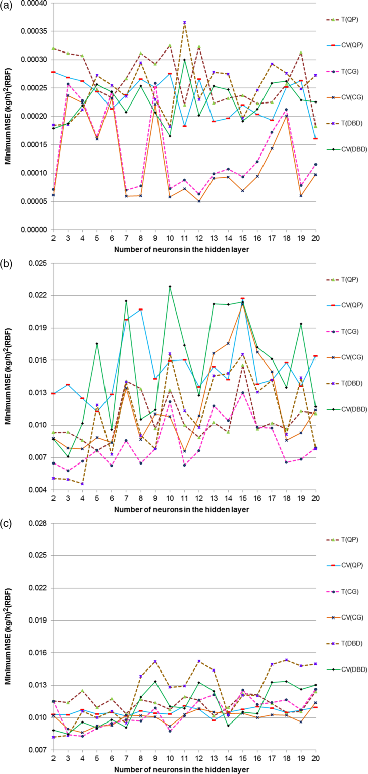
Figure 3. Minimum MSEs for the training and cross-validation of the RBFNs trained with CG, DBD and QP in the (a) climb, (b) cruise and (c) descent phase.

For the structures of the RBF networks with the best testing performance, the linear uppermost correlation coefficient was found to be 0.999882, 0.897204 and 0.952523 for the climb, cruise and descent flight phase, respectively. The values of the predefined types of error for the case of the RBF networks are presented in Table 3.

Table 3 Testing phase error values in fuel flow rate for the optimum RBF network architecture

Climb: CG-RBF, cruise: DBD-RBFN, descent: DBD-RBF.

3.3 ANFIS results

Applying fuzzy guidelines as a pre-processor to an ANN permits the integration of human awareness to carry out decision-making and inference. The ANFIS model optimises the fuzzy laws (membership role parameters) with back-proliferation, thus human knowledge is not required. To start the development of the ANFIS prediction model, a fuzzy model first has to be obtained. To define this model, it is necessary to determine the number of inputs and linguistic variables and, thereby, the number of laws for the final fuzzy model. As in the initial step for defining the initial fuzzy model, the subtractive clustering technique is used on the input–output data pairs. The technique proposed by Chiu^{(Reference Chiu24)} is a quick, one-pass algorithm for approximating the number of clusters and cluster centres using an unsupervised method by determining the prospective data points within the feature space. After this clustering process, the number of fuzzy rules and principle fuzzy membership functions are measured. Therefore, the optimal values of these parameters, as well as the resultant and premise parameters, are obtained using the learning algorithm.

In this study, the DBD, CG and QP learning algorithms were implemented for the ANFIS architecture, as in the situation of the RBFNs and MLP-ANNs. After trying numerous network parameters in a search for the most accurate testing outcomes, the following were selected for the execution of the ANFIS networks: no hidden layer configuration, three membership functions per network input, Gaussian-shaped curve fuzzy membership function, and TSK fuzzy model (the well-recognised Sugeno fuzzy model). For ANFIS networks, the MSE values achieved for the training and cross-validation using the DBD, CG and QP algorithms (with the latter having a momentum factor of 0.85) versus the number of epochs are shown in Fig. 4(a), (b) and (c) for the climb, cruise and descent flight phase, respectively. The lowest cross-validation MSE value of 5.892 × 10⁻⁵ was obtained at epoch number 492 when using the DBD training algorithm for the climb phase, whereas a lowest value of 0.010232367 was obtained at epoch number 740 when using the QP training algorithm for the descent phase, and 0.009143089 at epoch number 367 when using the DBD training algorithm for the cruise flight phase.

Figure 4. MSE versus number of epochs for the training and cross-validation of the ANFIS architectures trained with CG, DBD and QP in the (a) climb, (b) cruise and (c) descent phase.

Among the different ANFIS networks, the optimal testing result in terms of the linear correlation coefficient was 0.999799, 0.890047 and 0.922952 for the climb, cruise and descent flight phase, respectively. The error values for the best ANFIS configurations are reported in Table 4.

Table 4 Testing phase error values in fuel flow rate for the optimum ANFIS architecture

Climb: DBD-ANFIS, cruise: DBD-ANFIS, descent: QP-ANFIS.

Consequently, considering these testing results for the three ANN architectures, the output parameter values estimated for the optimal ANN architectures and the data acquired from the actual FDRs are also shown, considering the associated ANN dataset, in Fig. 5(a), (b) and (c) for the climb (RBF), cruise and descent phase, respectively. Considering the results shown in these figures, it can be concluded that there is a good fit between the real values and those predicted by the model for the fuel flow rate in each flight phase.

Figure 5. Test results of the best ANN architectures for the (a) climb (RBF), (b) cruise (MLP) and (c) descent (RBF) phase.

Figure 6. Fuel flow rate outputs produced by the most accurate ANNs in the (a) climb, (b) cruise and (c) descent phase.

The obtained ANN models were also employed to generate formerly inaccessible output values by feeding new input data into all the model networks. Yielding linear correlation coefficients extremely close to 1, the derived ANN models were extremely efficient for obtaining accurate new values for the fuel flow rate. The resulting outputs are shown versus the model inputs in Fig. 6(a)–(c).