2. Preliminaries

As mentioned in the introduction, the complete classifications of real hypersurfaces in complex two-plane Grassmannians ${G_2({\mathbb {C}}^{m+2})}$, $m \geq 3$, satisfying two invariant conditions for the distributions $\mathcal {C}^{\bot }=\mathrm {span}\{\xi \}$ and ${{\mathcal {Q}}^{\bot }}=\mathrm {span}\{\xi _{1}, \xi _{2}, \xi _{3}\}$ was given in [Reference Berndt and Suh4].

In fact, in [Reference Berndt3, Reference Berndt and Suh4] Berndt and Suh gave the characterizations of the singular unit normal vector $N$ of $M$ in complex two-plane Grassmannians ${G_2({\mathbb {C}}^{m+2})}$: There are two types of singular normal vector, those $N$ for which $JN \bot \mathcal {J} N$, and those for which $JN \in \mathcal {J} N$. In other words, it means that $\xi \in \mathcal {Q}$ or $\xi \in {{\mathcal {Q}}^{\bot }}$ because $JN=-\xi$, $\mathcal {J}N=\mathrm {span}\{\xi _{1}, \xi _{2}, \xi _{3}\}={{\mathcal {Q}}^{\bot }}$, and $TM=\mathcal {Q} \oplus {{\mathcal {Q}}^{\bot }}$. The following proposition tells us that the normal vector field $N$ on the model spaces of $(\mathcal {T}_{A})$ is singular of type of $JN \in \mathcal {J} N$, that is, $\xi \in {{\mathcal {Q}}^{\bot }}$.

Proposition A [Reference Berndt and Suh4, Reference Berndt and Suh9]

Let $(\mathcal {T}_{A})$ be the tube of radius $0 < r < \frac {\pi }{\sqrt {8}}$ around the totally geodesic ${G_2({\mathbb {C}}^{m+1})}$ in ${G_2({\mathbb {C}}^{m+2})}$. Then the following statements hold:

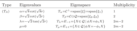
1. 1. $(\mathcal {T}_{A})$ is a Hopf hypersurface.

2. 2. Every unit normal vector field $N$ of $(\mathcal {T}_{A})$ is singular and of type $JN \in \mathcal {J} N$.

3. 3. The eigenvalues and their corresponding eigenspaces and multiplicities are given in Table 1.

4. 4. The Reeb flow on $(\mathcal {T}_{A})$ is isometric.

Table 1. Principal curvatures of a model space of type $(\mathcal {T}_{A})$

In proposition ${\rm A}$, the notion of isometric Reeb flow gave a kind of characterizations of real hypersurface of type $(\mathcal {T}_{A})$. Like for such an investigation, many geometric conditions were considered as characterizations of the model space of $(\mathcal {T}_{A})$ in complex two-plane Grassmannians (see [Reference Jeong, Pérez, Suh and Woo14, Reference Machado and Pérez22, Reference Machado and Pérez23, Reference Pérez25, Reference Pérez, Lee, Suh and Woo26, Reference Pérez, Suh and Woo28, Reference Suh, Lee and Kim39, Reference Suh, Lee and Kim40]).

On the other hand, by using the notion of isometric Reeb flow, that is, the shape operator $A$ of a Hopf real hypersurface $M$ in ${G_2({\mathbb {C}}^{m+2})}$ commutes with structure tensor $\phi$, that is, $A \phi = \phi A$, Berndt and Suh gave:

(2.1)\begin{equation} \begin{split} (\nabla_{X}A)Y & ={-} \eta(Y) \phi X +(X\alpha)\eta(Y) \xi + \alpha g(A \phi X, Y) \xi - g(A^{2} \phi X, Y) \xi \\ & \quad - \sum_{i=1}^{3}\big\{ \eta_{\nu}(Y)\phi_{\nu} X + g(\phi_{\nu} \xi, Y) \phi \phi_{\nu} X + 2g(\phi_{\nu} \xi, X) \phi \phi_{\nu} Y \\ & \quad + g(\phi_{\nu} \xi, X) \eta_{\nu} (Y) \xi - \eta_{\nu}(\xi) g(\phi_{\nu} X, Y) \xi + g(\phi_{\nu} X, Y){{\xi}_{\nu}} \\ & \quad - \eta(X)\eta_{\nu}(Y) \phi_{\nu} \xi + g(\phi_{\nu} \phi X, Y) \phi_{\nu} \xi \big \} \end{split} \end{equation}

for any tangent vector fields $X$ and $Y$ on $M$ (see proposition 4 in [Reference Berndt and Suh5]). In fact, from (iv) in proposition ${\rm A}$, we see that the shape operator $A$ of $(\mathcal {T}_{A})$ satisfies $A \phi = \phi A$. Thus, the above equation (2.1) holds on $(\mathcal {T}_{A})$ and it can be rearranged as

(2.2)\begin{equation} \begin{split} (\nabla_{X}A)Y & ={-} \eta(Y) \phi X + \alpha g(A \phi X, Y) \xi - g(A^{2} \phi X, Y) \xi \\ & \quad - \sum_{i=1}^{3}\big\{ \eta_{\nu}(Y)\phi_{\nu} X + g(\phi_{\nu} \xi, Y) \phi \phi_{\nu} X + 2g(\phi_{\nu} \xi, X) \phi \phi_{\nu} Y \\ & \quad + g(\phi_{\nu} \xi, X) \eta_{\nu} (Y) \xi - \eta_{\nu}(\xi) g(\phi_{\nu} X, Y) \xi + g(\phi_{\nu} X, Y){{\xi}_{\nu}} \\ & \quad - \eta(X)\eta_{\nu}(Y) \phi_{\nu} \xi + g(\phi_{\nu} \phi X, Y) \phi_{\nu} \xi \big \} \end{split} \end{equation}

for any tangent vector fields $X$ and $Y$ on $T(\mathcal {T}_{A})=T_{\alpha }\oplus T_{\beta }\oplus T_{\lambda }\oplus T_{\mu }$.

3. Fundamental equations of real hypersurfaces in ${G_2({\mathbb {C}}^{m+2})}$

We use some references [Reference Lee and Suh17, Reference Pérez and Suh27, Reference Suh34] to recall the Riemannian geometry of complex two-plane Grassmannians ${G_2({\mathbb {C}}^{m+2})}$, $m \geq 3$, and some fundamental formulas including the Codazzi and Gauss equations for a real hypersurface in ${G_2({\mathbb {C}}^{m+2})}$.

Let $M$ be a real hypersurface of complex two-plane Grassmannians ${G_2({\mathbb {C}}^{m+2})}$, $m \geq 3$, that is, a submanifold of ${G_2({\mathbb {C}}^{m+2})}$ with real codimension one. The induced Riemannian metric on $M$ will also be denoted by $g$, and $\nabla$ denotes the Riemannian connection of $(M,g)$. Let $N$ be a local unit normal field of $M$ in ${G_2({\mathbb {C}}^{m+2})}$ and $S$ the shape operator of $M$ with respect to $N$, that is, ${\bar \nabla }_{X}N = -SX$. The Kähler structure $J$ of complex two-plane Grassmannians ${G_2({\mathbb {C}}^{m+2})}$ induces on $M$ an almost contact metric structure $(\phi ,\xi ,\eta ,g)$. Furthermore, let $\{J_1, J_2, J_3 \}$ be a canonical local basis of the quaternionic Kähler structure ${\mathcal {J}}$. Then each $J_\nu$ induces an almost contact metric structure $(\phi _\nu ,\xi _\nu ,\eta _\nu ,g)$ on $M$. Now let us put

(3.1)\begin{equation} JX={{{\phi}}}X+{\eta}(X)N,\quad J_{\nu}X={{{\phi}}}_{\nu}X+{\eta}_{\nu}(X)N \end{equation}

for any tangent vector $X$ on a real hypersurface $M$ in ${G_2({\mathbb {C}}^{m+2})}$, where $N$ denotes a normal vector of $M$ in ${G_2({\mathbb {C}}^{m+2})}$. Then the following identities can be proved in a straightforward method and will be used frequently in subsequent calculations:

(3.2)\begin{equation} \begin{split} & {\phi}_{\nu +1}{\xi}_{\nu}={-}{\xi}_{{\nu}+2},\quad {\phi}_{\nu}{\xi}_{{\nu}+1}={\xi}_{{\nu}+2}, \quad {\phi}{\xi}_{\nu}={\phi}_{\nu}{\xi},\quad {\eta}_{\nu}({\phi}X)={\eta}({\phi}_{\nu}X),\\ & {\phi}_{\nu}{\phi}_{{\nu}+1}X={\phi}_{{\nu}+2}X+{\eta}_{{\nu}+1}(X){\xi}_{\nu}, \quad {\phi}_{{\nu}+1}{\phi}_{\nu}X={-}{\phi}_{{\nu}+2}X+{\eta}_{\nu}(X){\xi}_{{\nu}+1}, \end{split} \end{equation}

where we have used that $J_{\nu }J_{\nu +1}=J_{\nu +2}= - J_{\nu +1}J_{\nu }$.

On the other hand, from the parallelism of $J$ and $\mathcal {J}$ which are defined by

\begin{equation*} \bar \nabla_{X} J =0 \ \ \mathrm{and} \ \ \bar \nabla_{X}J_{\nu} = q_{\nu+2}(X)J_{\nu+1} - q_{\nu+1}(X) J_{\nu+2} \ (\nu \ \mathrm{mod}\ 3), \end{equation*}

together with Gauss and Weingarten formulas, it follows that

(3.3)\begin{gather} ({\nabla}_X{{{\phi}}})Y={\eta}(Y)AX-g(AX,Y){\xi},\quad {\nabla}_X{\xi}={{{\phi}}}AX, \end{gather}

(3.4)\begin{gather} {\nabla}_X{\xi}_{\nu}=q_{{\nu}+2}(X){\xi}_{{\nu}+1}-q_{{\nu}+1}(X){\xi}_{{\nu}+2} +{{{\phi}}}_{\nu}AX, \end{gather}

(3.5)\begin{gather} \begin{split} ({\nabla}_X{{{\phi}}}_{\nu})Y & ={-}q_{{\nu}+1}(X){{{\phi}}}_{{\nu}+2}Y+q_{{\nu}+2}(X){{{\phi}}}_{{\nu}+1}Y\\ & \quad + {\eta}_{\nu}(Y)AX -g(AX,Y){\xi}_{\nu}. \end{split} \end{gather}

Combining these formulas, we find the following

(3.6)\begin{equation} \begin{split} {\nabla}_X({{{\phi}}}_{\nu}{\xi}) & ={\nabla}_X({{{\phi}}}{\xi}_{\nu}) \\ & =({\nabla}_X{{{\phi}}}){\xi}_{\nu}+{{{\phi}}}({\nabla}_X{\xi}_{\nu})\\ & =q_{{\nu}+2}(X){{{\phi}}}_{{\nu}+1}{\xi}-q_{{\nu}+1}(X){{{\phi}}}_{{\nu}+2}{\xi}+{{{\phi}}}_{\nu}{{{\phi}}}AX \\ & \quad \ - g(AX,{\xi}){\xi}_{\nu}+{\eta}({\xi}_{\nu})AX. \end{split} \end{equation}

Moreover, from $JJ_{\nu }=J_{\nu }J$, ${\nu }=1,2,3$, it follows that

(3.7)\begin{equation} {{{\phi}}}{{{\phi}}}_{\nu}X={{{\phi}}}_{\nu}{{{\phi}}}X+{\eta}_{\nu}(X){\xi}-{\eta}(X){\xi}_{\nu}. \end{equation}

Finally, using the explicit expression for the Riemannian curvature tensor $\bar {R}$ of complex two-plane Grassmannians ${G_2({\mathbb {C}}^{m+2})}$ in the introduction, the Codazzi and Gauss equations of $M$ in ${G_2({\mathbb {C}}^{m+2})}$ are given respectively by

(3.8)\begin{equation} \begin{split} (\nabla_XA)Y - (\nabla_YA)X & = \eta(X)\phi Y - \eta(Y)\phi X - 2g(\phi X,Y)\xi \\ & \quad + \sum_{\nu=1}^{3} \big\{\eta_\nu(X)\phi_\nu Y - \eta_\nu(Y)\phi_\nu X - 2g(\phi_\nu X,Y)\xi_\nu\big\} \\ & \quad + \sum_{\nu=1}^{3} \big\{\eta_\nu(\phi X)\phi_\nu\phi Y - \eta_\nu(\phi Y)\phi_\nu\phi X\big\} \\ & \quad + \sum_{\nu=1}^{3} \big\{\eta(X)\eta_\nu(\phi Y) - \eta(Y)\eta_\nu(\phi X)\big\}\xi_{\nu} \end{split} \end{equation}

and

(3.9)\begin{equation} \begin{split} R(X,Y)Z & = g(Y,Z)X - g(X,Z)Y + g({\phi}Y,Z){\phi}X - g({\phi}X,Z){\phi}Y \\ & \quad - 2g({\phi}X,Y){\phi}Z+ g(AY,Z)AX - g(AX,Z)AY \\ & \quad + \sum_{\nu=1}^{3} \Big \{g({{\phi}_{\nu}}Y,Z){{\phi}_{\nu}}X - g({{\phi}_{\nu}}X,Z){{\phi}_{\nu}}Y - 2g({{\phi}_{\nu}}X,Y){{\phi}_{\nu}}Z \\ & \quad + g({{\phi}_{\nu}}{\phi}Y,Z){{\phi}_{\nu}} {\phi}X - g({{\phi}_{\nu}}{\phi}X,Z){{{\phi}_{\nu}}}{\phi}Y \\ & \quad + \eta(X){{{\eta}_{\nu}}}(Z){{{\phi}_{\nu}}}{\phi}Y - {\eta}(Y){{{\eta}_{\nu}}}(Z){{{\phi}_{\nu}}}{\phi}X \\ & \quad + {\eta}(Y)g({{{\phi}_{\nu}}}{\phi}X,Z){{\xi}_{\nu}} - {\eta}(X)g({{{\phi}_{\nu}}}{\phi}Y,Z){{{\xi}_{\nu}}} \Big \} \end{split} \end{equation}

for any tangent vector fields $X$, $Y$ and $Z$ on $M$.

On the other hand, we can derive some important facts from the geometric condition of $M$ being Hopf, that is, $A\xi = \alpha \xi$ where $\alpha = g(A\xi , \xi )$. Among them, we introduce the following formulas which are induced from the Codazzi equation:

Lemma A [Reference Berndt and Suh5]

If $M$ is a connected orientable Hopf real hypersurface in complex two-plane Grassmannians ${G_2({\mathbb {C}}^{m+2})}$, $m \geq 3$, then

(3.10)\begin{equation} \mathrm{grad} \, \alpha = (\xi \alpha)\xi + 4\sum_{\nu=1}^{3} \eta_{\nu}(\xi)\phi_{\nu} \xi \end{equation}

and

(3.11) \begin{equation} \begin{split} & 2 A \phi A X - \alpha A\phi X - \alpha \phi A X \\ & \quad = 2 \phi X + 2 \sum_{\nu=1}^{3} \big\{ \eta_{\nu} (X) \phi_{\nu} \xi - g(\phi_{\nu}\xi, X) \xi_{\nu} + \eta_{\nu} (\xi) \phi_{\nu} X \big\} \\ & \quad \quad -4 \sum_{\nu=1}^{3} \big \{ \eta(X) \eta_{\nu} (\xi) \phi_{\nu} \xi - \eta_{\nu}(\xi) g(\phi_{\nu} \xi, X) \xi \big\} \end{split} \end{equation}

for any tangent vector field $X$ on $M$ in ${G_2({\mathbb {C}}^{m+2})}$.

4. Proof of theorem 1

Let $M$ be a Hopf real hypersurface with cyclic parallel structure Jacobi operator in complex two-plane Grassmannians ${G_2({\mathbb {C}}^{m+2})}$, $m \geq 3$.

From (3.9) the structure Jacobi operator ${R_{\xi }} \in \mathrm {End}(TM)$ is given as follows

(4.1)\begin{equation} \begin{split} R_{\xi}(Y) & = R(Y,\xi)\xi \\ & = Y - \eta(Y) \xi + \alpha AY - \alpha^{2} \eta(Y) \xi \\ & \quad - \sum_{\nu=1}^{3} \big\{ \eta_{\nu}(Y) {{\xi}_{\nu}} - \eta(Y) \eta_{\nu}(\xi) {{\xi}_{\nu}} - 3g(\phi_{\nu} \xi, Y) \phi_{\nu} \xi + \eta_{\nu}(\xi) \phi_{\nu} \phi Y \big \} \end{split} \end{equation}

for any tangent vector field $Y \in TM$ (see [Reference Lee and Suh19, Reference Machado, Pérez and Suh24]).

Taking the covariant derivative of (4.1) along the direction of $X$ implies

(4.2)\begin{equation} \begin{split} (\nabla_{X}R_{\xi})Y & = \nabla_{X}({R_{\xi}}Y) - {R_{\xi}} (\nabla_{X}Y) \\ & ={-}g(\phi AX, Y) \xi - \eta(Y) \phi AX \\ & \quad - \sum_{\nu=1}^{3} \Big [ g(\phi_{\nu} AX, Y) {{\xi}_{\nu}} + 2\eta(Y) g(\phi_{\nu} \xi, AX) {{\xi}_{\nu}} + \eta_{\nu}(Y) \phi_{\nu} AX \\ & \quad + 3 g(\phi_{\nu} AX, \phi Y) \phi_{\nu} \xi + 3 \eta(Y) \eta_{\nu}(AX) \phi_{\nu} \xi \\ & \quad - 3g(\phi_{\nu} \xi, Y) \phi_{\nu} \phi AX + 3 \alpha \eta (X) g(\phi_{\nu} \xi, Y) {{\xi}_{\nu}} \\ & \quad - 4 \eta_{\nu}(\xi) g(\phi_{\nu} \xi, Y) AX - 4 \eta_{\nu}(\xi)g(AX, Y) \phi_{\nu} \xi \\ & \quad - 2g(\phi_{\nu} \xi, AX) \phi_{\nu}\phi Y \Big ] \\ & \quad + g((\nabla_{X}A)\xi, \xi)AY + \alpha (\nabla_{X}A)Y - \alpha g((\nabla_{X}A)Y, \xi)\xi \\ & \quad - \alpha g(AY, \phi AX) \xi - \alpha \eta(Y) (\nabla_{X}A) \xi - \alpha \eta(Y) A \phi AX \end{split} \end{equation}

for any tangent vector fields $X$ and $Y$ on $M$ (see [Reference Lee and Suh19]). From this and using symmetric property of the structure Jacobi operator ${R_{\xi }}$ in ${G_2({\mathbb {C}}^{m+2})}$, the cyclic parallelism of the structure Jacobi operator (1.4) can be rearranged as follows:

(4.3) \begin{align} 0 & = g\big((\nabla_{X}{R_{\xi}})Y, Z \big) + g\big((\nabla_{Y}{R_{\xi}})Z, X \big)+g\big((\nabla_{Z}{R_{\xi}})X, Y \big)\nonumber\\ & = g\big((\nabla_{X}{R_{\xi}})Y, Z \big) + g\big((\nabla_{Y}{R_{\xi}})X, Z \big)\nonumber \\ & \quad + g(A\phi X, Z) \eta(Y) + \eta(X) g(A \phi Y, Z) + (\xi \alpha) g(AX, Y)\eta(Z)\nonumber \\ & \quad - \alpha (\xi \alpha) \eta(X) \eta(Y) \eta(Z) + \alpha^{2} \eta(Y) g(A \phi X, Z) - \alpha \eta(Y) g(A \phi A X, Z)\nonumber \\ & \quad + \alpha \eta(Y) g(A \phi AX, Z) + \alpha \eta(X) g(A \phi AY, Z) - \alpha (\xi \alpha) \eta(X) \eta(Y) \eta(Z)\nonumber \\ & \quad + \alpha^{2} \eta(X) g(A \phi Y, Z) - \alpha \eta(X) g(A \phi A Y, Z) + \alpha g((\nabla_X A)Y, Z)\nonumber \\ & \quad + \alpha g( \phi X, Y)\eta(Z) + \alpha \eta(X)g(\phi Y, Z) + 2\alpha \eta(Y) g(\phi X, Z) \nonumber \\ & \quad + \sum_{\nu=1}^{3} \Big [ \eta_{\nu}(Y) g(A \phi_{\nu} X, Z) - 2\eta(X)\eta_{\nu}(Y) g(A \phi_{\nu} \xi, Z) + \eta_{\nu}(X) g(A \phi_{\nu} Y, Z) \nonumber\\ & \quad + 3g(\phi_{\nu} \xi, Y) g(A \phi_{\nu} \phi X, Z) - 3 \eta(X) g(\phi_{\nu} \xi, Y) g(A{{\xi}_{\nu}}, Z)\nonumber \\ & \quad + 3g(\phi_{\nu} \xi, X) g(A \phi \phi_{\nu} Y, Z) - 3 \alpha g(\phi_{\nu} \xi, X) \eta_{\nu}(Y)\eta(Z)\nonumber \\ & \quad + 4 \eta_{\nu}(\xi) g(\phi_{\nu} \xi, X) g(AY, Z) + 4 \eta_{\nu}(\xi) g(\phi_{\nu} \xi, Y)g(AX, Z)\nonumber\\ & \quad + 2 g(\phi_{\nu}\phi X, Y)g(A \phi_{\nu} \xi, Z) + 4 g(AX, Y) \eta_{\nu}(\xi) g(\phi_{\nu} \xi, Z)\nonumber\\ & \quad - 4 \alpha \eta(X) \eta(Y) \eta_{\nu}(\xi) g(\phi_{\nu} \xi, Z) - 4 \alpha \eta(X) \eta(Y) \eta_{\nu}(\xi) g(\phi_{\nu} \xi, Z) \Big ]\nonumber \\ & \quad + \alpha \sum_{\nu=1}^{3} \Big [ g(\phi_\nu X, Y)\eta_\nu(Z) + \eta_\nu(X)g(\phi_\nu Y, Z) + 2\eta_{\nu}(Y) g(\phi_\nu X,Z)\nonumber \\ & \quad - g(\phi_\nu\phi X, Y)g(\phi_{\nu} \xi, Z) + g(\phi_{\nu} \xi, X)g(\phi \phi_\nu Y, Z)\nonumber \\ & \quad + \eta_\nu(\phi X)\eta_{\nu}(Y) \eta(Z) + \eta(X)\eta_{\nu}(Y) g(\phi_{\nu} \xi, Z)\Big ], \end{align}

where we have used

\begin{equation*} \begin{split} g((\nabla_{Z}A)\xi, X) & = (Z \alpha) \eta(X) - \alpha g(A \phi X, Z) + g(A \phi A X, Z) \\ & = (\xi \alpha) \eta(Z) \eta(X) + 4 \sum_{\nu=1}^{3} \eta_{\nu}(\xi) g(\phi_{\nu} \xi, Z) \eta(X) \\ & \quad \ - \alpha g(A \phi X, Z) + g(A \phi A X, Z) \end{split} \end{equation*}

and

\begin{equation*} \begin{split} & g((\nabla_ZA)X, Y) \\ & = g((\nabla_X A)Z, Y) + \eta(Z)g( \phi X, Y) - \eta(X)g(\phi Z, Y) - 2g(\phi Z,X)\eta(Y) \\ & \quad + \sum_{\nu=1}^{3} \big\{\eta_\nu(Z)g(\phi_\nu X, Y) - \eta_\nu(X)g(\phi_\nu Z, Y) - 2g(\phi_\nu Z,X)\eta_{\nu}(Y) \big\} \\ & \quad + \sum_{\nu=1}^{3} \big\{\eta_\nu(\phi Z)g(\phi_\nu\phi X, Y) - \eta_\nu(\phi X)g(\phi_\nu\phi Z, Y) \big\} \\ & \quad + \sum_{\nu=1}^{3} \big\{\eta(Z)\eta_\nu(\phi X) - \eta(X)\eta_\nu(\phi Z)\big\}\eta_{\nu}(Y) \end{split} \end{equation*}

for any tangent vector fields $X$, $Y$ and $Z$ on $M$. Deleting $Z$ from (4.3) and using (4.2) gives

(4.4)\begin{align} & -g(\phi AX, Y) \xi - \eta(Y) \phi AX -g(\phi AY, X) \xi - \eta(X) \phi AY + \eta(Y)A\phi X \nonumber\\ & + \eta(X) A \phi Y + (\xi \alpha) g(AX, Y) \xi - 2 \alpha (\xi \alpha) \eta(X) \eta(Y) \xi + \alpha^{2} \eta(Y) A \phi X \nonumber\\ & + \alpha^{2} \eta(X) A \phi Y + \alpha (\nabla_X A)Y + \alpha g(\phi X, Y)\xi + \alpha \eta(X) \phi Y + 2\alpha \eta(Y) \phi X \nonumber\\ & - \sum_{\nu=1}^{3} \Big [ g(\phi_{\nu} AX, Y) {{\xi}_{\nu}} + 2\eta(Y) g(\phi_{\nu} \xi, AX) {{\xi}_{\nu}} + \eta_{\nu}(Y) \phi_{\nu} AX \nonumber\\ & +3 g(\phi_{\nu} AX, \phi Y) \phi_{\nu} \xi + 3 \eta(Y) \eta_{\nu}(AX) \phi_{\nu} \xi - 3g(\phi_{\nu} \xi, Y) \phi_{\nu} \phi AX \nonumber\\ &+ 3 \alpha \eta (X) g(\phi_{\nu} \xi, Y) {{\xi}_{\nu}} - 4 \eta_{\nu}(\xi) g(\phi_{\nu} \xi, Y) AX \nonumber\\ & \quad \quad \quad - 4 \eta_{\nu}(\xi)g(AX, Y) \phi_{\nu} \xi - 2g(\phi_{\nu} \xi, AX) \phi_{\nu}\phi Y \nonumber\\ &+ g(\phi_{\nu} AY, X) {{\xi}_{\nu}} + 2\eta(X) g(\phi_{\nu} \xi, AY) {{\xi}_{\nu}} + \eta_{\nu}(X) \phi_{\nu} AY \nonumber\\ &+3 g(\phi_{\nu} AY, \phi X) \phi_{\nu} \xi + 3 \eta(X) \eta_{\nu}(AY) \phi_{\nu} \xi - 3g(\phi_{\nu} \xi, X) \phi_{\nu} \phi AY \nonumber\\ & + 3 \alpha \eta (Y) g(\phi_{\nu} \xi, X) {{\xi}_{\nu}} - 4 \eta_{\nu}(\xi) g(\phi_{\nu} \xi, X) AY \nonumber\\ & - 4 \eta_{\nu}(\xi)g(AY, X) \phi_{\nu} \xi - 2g(\phi_{\nu} \xi, AY) \phi_{\nu}\phi X \Big ] \nonumber\\ & + \sum_{\nu=1}^{3} \Big [ \eta_{\nu}(Y) A \phi_{\nu} X - 2\eta(X)\eta_{\nu}(Y) A \phi_{\nu} \xi + \eta_{\nu}(X) A \phi_{\nu} Y \nonumber\\ &+ 3g(\phi_{\nu} \xi, Y) A \phi_{\nu} \phi X - 3 \eta(X) g(\phi_{\nu} \xi, Y) A{{\xi}_{\nu}} \nonumber\\ &+ 3g(\phi_{\nu} \xi, X) A \phi \phi_{\nu} Y - 3 \alpha g(\phi_{\nu} \xi, X) \eta_{\nu}(Y)\xi \nonumber\\ &+ 4 \eta_{\nu}(\xi) g(\phi_{\nu} \xi, X) AY + 4 \eta_{\nu}(\xi) g(\phi_{\nu} \xi, Y) AX \nonumber\\ &+ 2 g(\phi_{\nu}\phi X, Y) A \phi_{\nu} \xi + 4 g(AX, Y)\eta_{\nu}(\xi) \phi_{\nu} \xi \nonumber\\ &- 4 \alpha \eta(X) \eta(Y) \eta_{\nu}(\xi) \phi_{\nu} \xi - 4 \alpha \eta(X) \eta(Y) \eta_{\nu}(\xi) \phi_{\nu} \xi \Big ] \nonumber\\ & + \alpha \sum_{\nu=1}^{3} \Big [ g(\phi_\nu X, Y) {{\xi}_{\nu}} + \eta_\nu(X) \phi_\nu Y + 2\eta_{\nu}(Y) \phi_\nu X - g(\phi_\nu\phi X, Y) \phi_{\nu} \xi\nonumber\\ & + g(\phi_{\nu} \xi, X) \phi \phi_\nu Y + \eta_\nu(\phi X)\eta_{\nu}(Y) \xi + \eta(X)\eta_{\nu}(Y) \phi_{\nu} \xi \Big ]\nonumber\\ & + g((\nabla_{X}A)\xi, \xi)AY - \alpha g((\nabla_{X}A)Y, \xi)\xi - \alpha g(AY, \phi AX) \xi \nonumber\\ & - \alpha \eta(Y) A \phi AX + g((\nabla_{Y}A)\xi, \xi)AX - \alpha g((\nabla_{Y}A)X, \xi)\xi \nonumber\\ & - \alpha g(AX, \phi AY) \xi - \alpha \eta(X) A \phi AY + \alpha (\nabla_{X}A)Y - \alpha \eta(Y) (\nabla_{X}A) \xi \nonumber\\ & + \alpha (\nabla_{Y}A)X - \alpha \eta(X) (\nabla_{Y}A) \xi =0. \end{align}

On the other hand, by using the Codazzi equation (3.8) and (3.10) in the latter part of (4.4), we obtain

(4.5)\begin{align} & g((\nabla_{X}A)\xi, \xi)AY - \alpha g((\nabla_{X}A)Y, \xi)\xi - \alpha g(AY, \phi AX) \xi - \alpha \eta(Y) A \phi AX\nonumber\\ & + g((\nabla_{Y}A)\xi, \xi)AX - \alpha g((\nabla_{Y}A)X, \xi)\xi - \alpha g(AX, \phi AY) \xi - \alpha \eta(X) A \phi AY\nonumber\\ & + \alpha (\nabla_{X}A)Y + \alpha (\nabla_{Y}A)X - \alpha \eta(Y) (\nabla_{X}A) \xi - \alpha \eta(X) (\nabla_{Y}A) \xi\nonumber\\ & = (\xi \alpha) \eta(X) AY + 4 \sum_{\nu=1}^{3} \eta_{\nu}(\xi) g(\phi_{\nu} \xi, X) AY - \alpha g(A\phi AX, Y) \xi \nonumber\\ & \quad - \alpha \eta(Y) A \phi AX -\alpha (\xi \alpha) \eta(X) \eta(Y)\xi - 4\alpha \sum_{\nu=1}^{3} \eta_{\nu}(\xi) g(\phi_{\nu} \xi, X) \eta(Y)\xi \nonumber\\ & \quad - \alpha^{2} g(\phi AX,Y) \xi + \alpha g(A \phi AX, Y) \xi + (\xi \alpha) \eta(Y) AX \nonumber\\ & \quad + 4 \sum_{\nu=1}^{3} \eta_{\nu}(\xi) g(\phi_{\nu} \xi, Y) AX + \alpha g(A\phi AX, Y) \xi \nonumber\\ & \quad - \alpha \eta(X) A \phi AY -\alpha (\xi \alpha) \eta(X) \eta(Y) \xi \nonumber\\ & \quad -4 \alpha \sum_{\nu=1}^{3} \eta_{\nu}(\xi) \eta(X) g(\phi_{\nu} \xi, Y) \xi - \alpha^{2} g(\phi AY,X)\xi + \alpha g(A \phi AY, X) \xi \nonumber\\ & \quad + 2 \alpha (\nabla_X A)Y + \alpha \eta(Y)\phi X - \alpha \eta(X)\phi Y - 2\alpha g(\phi Y,X)\xi \nonumber\\ & \quad+ \alpha \sum_{\nu=1}^{3} \big \{ \eta_\nu(Y)\phi_\nu X - \eta_\nu(X)\phi_\nu Y - 2g(\phi_\nu Y,X)\xi_\nu \eta_\nu(\phi Y)\phi_\nu\phi X \big \}\nonumber\\ & \quad + \alpha \sum_{\nu=1}^{3} \big \{ - \eta_\nu(\phi X)\phi_\nu\phi Y + \eta(Y)\eta_\nu(\phi X){{\xi}_{\nu}} - \eta(X)\eta_\nu(\phi Y)\xi_{\nu} \big \}\nonumber\\ & \quad-\alpha \eta(Y) \{(\xi \alpha) \eta(X) \xi + 4 \sum_{\nu=1}^{3} \eta_{\nu}(\xi) g(\phi_{\nu} \xi, X) \xi + \alpha \phi AX - A\phi AX \big \}\nonumber\\ & \quad-\alpha \eta(X) \{(\xi \alpha) \eta(Y) \xi + 4 \sum_{\nu=1}^{3} \eta_{\nu}(\xi) g(\phi_{\nu} \xi, Y) \xi + \alpha \phi AY - A\phi AY \big \}. \end{align}

From now on, we want to prove that the normal vector field $N$ of a Hopf real hypersurface $M$ in ${G_2({\mathbb {C}}^{m+2})}$ is singular. Then by the meaning of singularity mentioned in the introduction, we see that either $\xi \in \mathcal {Q}$ or $\xi \in {{\mathcal {Q}}^{\bot }}$ where $\mathcal {Q}$ is the maximal quaternionic subbundle of $TM = \mathcal {Q} \oplus {{\mathcal {Q}}^{\bot }}$. In order to do this, we may put the Reeb vector field $\xi$ as follows:

(*)\begin{equation} \xi = \eta(X_{0}){X_{0}} + \eta({{\xi}_1}) {{\xi}_1} \end{equation}

for unit vector fields ${X_{0}} \in \mathcal {Q}$ and ${{\xi }_1} \in {{\mathcal {Q}}^{\bot }}$ with $\eta ({X_{0}}) \eta ({{\xi }_1}) \neq 0$. By using the notation (*) we obtain that the Reeb function $\alpha$ is constant along the direction of $\xi$ if and only if the distribution $\mathcal {Q}$- or the $\mathcal {Q}^{\bot }$-component of the structure vector field $\xi$ is invariant by the shape operator, that is $A {X_{0}} = \alpha {X_{0}}$ and $A {{\xi }_1} = \alpha {{\xi }_1}$ (see [Reference Jeong, Machado, Pérez and Suh13, Reference Lee and Suh18]). From this fact, we obtain the following useful formulas for Hopf real hypersurfaces in ${G_2({\mathbb {C}}^{m+2})}$.

Proof. Putting $X = {X_{0}}$ in (3.11) and using $A{X_{0}} = \alpha {X_{0}}$, it yields

(4.6)\begin{equation} \begin{split} & \alpha A \phi {X_{0}} = \alpha^{2} \phi {X_{0}} + 2 \phi {X_{0}} + 2 \eta ({{\xi}_1}) \phi_{1} {X_{0}} -4 \eta({X_{0}}) \eta (\xi_{1}) \phi_{1} \xi ,\end{split} \end{equation}

where we have used $g(\phi _{\nu } \xi , {X_{0}}) =0$ for $\nu =1,2,3$ and $\eta _{2}(\xi ) = \eta _{3}(\xi )=0$.

On the other hand, by (*) we obtain

(4.7)\begin{equation} \phi_{1} \xi = \eta({X_{0}}) \phi_{1} {X_{0}} + \eta({{\xi}_1}) \phi_{1} {{\xi}_1} = \eta({X_{0}}) \phi_{1} {X_{0}}. \end{equation}

In addition, from (*) and $\phi _{1} \xi = \phi _{1} \xi$ we have

\begin{equation*} \begin{split} 0 = \phi \xi & = \eta({X_{0}}) \phi {X_{0}} + \eta({{\xi}_1}) \phi {{\xi}_1} \\ & = \eta({X_{0}}) \phi {X_{0}} + \eta({{\xi}_1}) \phi_{1} \xi \\ & = \eta({X_{0}}) \phi {X_{0}} + \eta({{\xi}_1}) \eta({X_{0}}) \phi_{1} {X_{0}}, \end{split} \end{equation*}

which means

(4.8)\begin{equation} \phi {X_{0}} ={-} \eta({{\xi}_1}) \phi_{1} {X_{0}} \end{equation}

because of $\eta ({X_{0}}) \eta ({{\xi }_1})\neq 0$. Substituting (4.7) and (4.8) to (4.6), we get

\begin{equation*} \alpha A \phi {X_{0}} = \alpha^{2} \phi {X_{0}} + 4 \eta^{2}({X_{0}}) \phi {X_{0}} = (\alpha^{2} + 4 \eta^{2}({X_{0}})) \phi {X_{0}}. \end{equation*}

Since $M$ has non-vanishing geodesic Reeb flow, we see that the vector field $\phi {X_{0}}$ is principal with corresponding principal curvature $\mu = ({\alpha ^{2}+ 4 \eta ^{2}({X_{0}})}/{\alpha })$.

Similarly, using (4.7) and (4.8), together with $\eta ({X_{0}}) \eta ({{\xi }_1}) \neq 0$, the formula (4.6) gives (b) and (c).

When the Reeb function $\alpha$ is vanishing, Pérez and Suh gave the following

Remark 4.2 By using the method in the proof of lemma ${\rm B}$, we can assert that if $M$ is a Hopf real hypersurface with constant Reeb curvature, then the unit normal vector field $N$ of $M$ is singular. In fact, since $M$ has constant Reeb function, (3.10) becomes

\[ 4 \sum_{\nu=1}^{3} \eta_{\nu}(\xi) \phi_{\nu} \xi=0 \]

By using (*), this equation yields $\eta ({{\xi }_1}) \phi _{1} \xi =0$. From our assumption of $\eta (X)\eta ({{\xi }_1}) \neq 0$ and (4.7), it leads to $\phi _{1} {X_{0}} =0$. Taking the inner product with $\phi _{1} {X_{0}}$, it implies

\[ g(\phi_{1} {X_{0}}, \phi_{1} {X_{0}}) ={-} g(\phi_{1} ^{2}{X_{0}}, {X_{0}}) = g({X_{0}}, {X_{0}}) - \big(\eta_{1}({X_{0}})\big)^{2}= 1, \]

which gives us a contradiction.

By using lemma ${\rm B}$, in the latter part of this section, we prove that the normal vector field $N$ of $M$ is singular, when a Hopf real hypersurface $M$ in ${G_2({\mathbb {C}}^{m+2})}$ has non-vanishing geodesic Reeb flow $\alpha =g(A\xi , \xi )$.

Proof. In [Reference Lee and Loo16], Lee and Loo show that if $M$ is Hopf, then the Reeb function $\alpha$ is constant along the direction of structure vector field $\xi$, that is, $\xi \alpha =0$. Then we see that the distribution $\mathcal {Q}$- and the $\mathcal {Q}^{\bot }$-component of $\xi$ are invariant by the shape operator $A$, that is $A{X_{0}} = \alpha {X_{0}}$ and $A{{\xi }_1} = \alpha {{\xi }_1}$.

Bearing in mind of these facts, putting $X={X_{0}}$ and $Y= {{\xi }_1}$ in (4.4) and using (4.5), we obtain

\begin{equation*} \begin{split} & \quad - \alpha \eta({X_{0}}) \phi {{\xi}_1} + \mu \eta({{\xi}_1}) \phi {X_{0}} + \mu \eta({X_{0}}) \phi {{\xi}_1} + 3\alpha (\nabla_{{X_{0}}} A){{\xi}_1} + 2\alpha \eta({{\xi}_1}) \phi {X_{0}} \\ & \quad -\alpha^{3} \eta({{\xi}_1}) \phi {X_{0}} + \mu \alpha^{2} \eta({{\xi}_1}) \phi {X_{0}} - \alpha^{3} \eta({X_{0}}) \phi {{\xi}_1} + \mu \alpha^{2} \eta({X_{0}}) \phi {{\xi}_1} \\ & \quad + \sum_{\nu=1}^{3} \Big [ \alpha \eta_{\nu}({{\xi}_1}) \phi_{\nu} {X_{0}} - 3 \alpha g(\phi_{\nu} {X_{0}}, \phi {{\xi}_1}) \phi_{\nu} \xi - 2 \alpha \eta({X_{0}}) \eta_{\nu}({{\xi}_1}) \phi_{\nu} \xi + \eta_{\nu}({{\xi}_1}) A \phi_{\nu} {X_{0}} \\ & \quad \quad \quad \quad - 2\eta({X_{0}})\eta_{\nu}({{\xi}_1}) A \phi_{\nu} \xi - 8 \alpha \eta({X_{0}}) \eta({{\xi}_1}) \eta_{\nu}(\xi) \phi_{\nu} \xi + \alpha \eta_\nu({{\xi}_1})\phi_\nu {X_{0}} \Big ] =0, \end{split} \end{equation*}

where we have used $g(\phi {{\xi }_1}, {X_{0}}) = - g(\phi {X_{0}}, {{\xi }_1})=0$ and

\[ g(\phi_{\nu} {X_{0}}, {{\xi}_1}) = g(\phi_{\nu} \xi, {X_{0}}) = g(\phi_{\nu} \xi, {{\xi}_1}) = g(\phi_{\nu}\phi {X_{0}}, {{\xi}_1}) =0 \]

for all $\nu =1,2,3$. Since $\eta _{2}(\xi )=\eta _{3}(\xi )=0$, together with $g(\phi _{1} {X_{0}}, \phi _{1} {X_{0}}) = 1$, this equation can be rearranged as

(4.9)\begin{equation} \begin{split} & - \alpha \eta({X_{0}}) \phi {{\xi}_1} + \mu \eta({{\xi}_1}) \phi {X_{0}} + \mu \eta({X_{0}}) \phi {{\xi}_1} + 3\alpha (\nabla_{{X_{0}}} A){{\xi}_1} \\ & + 2\alpha \eta({{\xi}_1}) \phi {X_{0}} -\alpha^{3} \eta({{\xi}_1}) \phi {X_{0}} + \mu \alpha^{2} \eta({{\xi}_1}) \phi {X_{0}} \\ & - \alpha^{3} \eta({X_{0}}) \phi {{\xi}_1} + \mu \alpha^{2} \eta({X_{0}}) \phi {{\xi}_1} + 2 \alpha \phi_{1} {X_{0}} - 5 \alpha \eta({X_{0}}) \phi \xi_{1}\\ & + \mu \phi_{1} {X_{0}} - 2\mu \eta({X_{0}}) \phi_{1} \xi - 8 \alpha \eta({X_{0}}) \big(\eta({{\xi}_1})\big)^{2} \phi_{1} \xi =0. \end{split} \end{equation}

From (4.7) and (4.8), (4.9) becomes

(4.10)\begin{equation} \begin{split} & \eta^{2}({X_{0}}) \big \{ - 6\alpha - \mu - \alpha^{3} + \mu \alpha^{2} - 8 \alpha \eta^{2}({{\xi}_1}) \big\}\phi_{1} {X_{0}} \\ & \quad - \eta^{2}({{\xi}_1})\big \{ \mu + 2\alpha -\alpha^{3} + \mu \alpha^{2} \big \} \phi_{1} {X_{0}} \\ & \quad + ( 2 \alpha + \mu ) \phi_{1} {X_{0}} + 3\alpha (\nabla_{{X_{0}}} A){{\xi}_1} =0. \end{split} \end{equation}

On the other hand, from (3.4) and (3.10), the assumption $A{{\xi }_1} = \alpha {{\xi }_1}$ yields

\begin{equation*} \begin{split} (\nabla_{X}A)\xi_{1} & = (X \alpha) {{\xi}_1} + \alpha \nabla_{X}{{\xi}_1} - A(\nabla_{X}{{\xi}_1}) \\ & = 4\eta({{\xi}_1}) g(\phi_{1} \xi, X) {{\xi}_1} + \alpha \{ q_{3}(X) {{\xi}_2} - q_{2}(X) {{\xi}_3} + \phi_{1} AX\} \\ & \quad \ - q_{3}(X) A{{\xi}_2} + q_{2}(X) A{{\xi}_3} - A\phi_{1} AX \end{split} \end{equation*}

for any tangent vector field $X$ on $M$. From this, taking the inner product with $\phi _{1} {X_{0}}$ to (4.10) and (3.4), together with $\alpha \mu = \alpha ^{2}+ 4 \eta ^{2}({X_{0}})$, we get

(4.11)\begin{equation} \begin{split} & \eta^{2}({X_{0}}) \big \{ - 14 \alpha - \mu + 12 \alpha \eta^{2}({X_{0}})\big\} - \eta^{2}({{\xi}_1})\big \{ \mu + 2\alpha + 4 \alpha \eta^{2}({X_{0}}) \big \} \\ & \quad + 2 \alpha + \mu -12 \alpha \eta^{2}({X_{0}})=0, \end{split} \end{equation}

where we have used $g(\phi _{1} {X_{0}}, \phi _{1} {X_{0}}) = 1$, $\eta ^{2}({X_{0}}) + \eta ^{2}({{\xi }_1})=1$, and

\begin{equation*} \begin{split} g((\nabla_{{X_{0}}}A)\xi_{1}, \phi_{1} {X_{0}}) & = \alpha g(\phi_{1} A{X_{0}}, \phi_{1}{X_{0}}) - g(A\phi_{1} A{X_{0}}, \phi_{1}{X_{0}}) \\ & = \alpha^{2} - \alpha \mu ={-}4 \eta^{2}({X_{0}}). \end{split} \end{equation*}

By using non-vanishing Reeb function $\alpha \neq 0$ and $\alpha \mu = \alpha ^{2}+ 4 \eta ^{2}({X_{0}})$, together with $\eta ^{2}({{\xi }_1}) = 1 - \eta ^{2}({X_{0}})$, (4.11) becomes

(4.12)\begin{equation} \begin{split} \eta^{2}({X_{0}}) \big \{ - 28 \alpha^{2} + 16 \alpha^{2}\eta^{2}({X_{0}}) \big\} =0. \end{split} \end{equation}

By virtue of 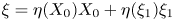$\xi = \eta ({X_{0}}) {X_{0}} + \eta ({{\xi }_1}){{\xi }_1}$ in (*) for $\eta ({X_{0}})\eta ({{\xi }_1}) \neq 0$, and our assumption of non-vanishing geodesic Reeb flow, that is, $\alpha \neq 0$, (4.12) implies that $\eta ^{2} ({X_{0}}) = \frac {7}{4}$. Since the structure vector field $\xi$ is unit, we should have $\eta ^{2}({X_{0}})+ \eta ^{2}({{\xi }_1}) =1$. From these facts, we obtain $\eta ^{2}({{\xi }_1}) =~- \frac {3}{4}$. It makes a contradiction. This means that either $\xi =\eta ({X_{0}}){X_{0}} = \pm {X_{0}} \in \mathcal {Q}$ or $\xi =\eta ({{\xi }_1}){{\xi }_1} = \pm {{\xi }_1} \in {{\mathcal {Q}}^{\bot }}$, which gives the unit normal vector field $N$ is singular.

Summing up lemmas ${\rm B}$ and 4.3, we assert that our theorem 1 in the introduction.

5. Cyclic parallel structure Jacobi operator for $JN \in \mathcal {J} N$

Hereafter, let $M$ be a Hopf real hypersurface with cyclic parallel structure Jacobi operator in complex two-plane Grassmannians ${G_2({\mathbb {C}}^{m+2})}$ for $m \geq 3$. Then by theorem 1, our discussions can be divided into two cases accordingly as the Reeb vector field $\xi \in {{\mathcal {Q}}^{\bot }}$ or $\xi \in \mathcal {Q}$.

In this section, we consider the case of $\xi \in {{\mathcal {Q}}^{\bot }}$ (i.e. $JN \in \mathcal {J} N$ where $N$ is a unit normal vector field on $M$ in ${G_2({\mathbb {C}}^{m+2})}$, $m \geq 3$). Since ${{\mathcal {Q}}^{\bot }}$ is 3-dimensional distribution defined by ${{\mathcal {Q}}^{\bot }} = \mathrm {span}\{{{\xi }_1}, {{\xi }_2}, {{\xi }_3} \}$, we may put $\xi = {{\xi }_1}$. From this, we give an important lemma as follows.

Lemma 5.1 Let $M$ be a real hypersurface in complex two-plane Grassmannians ${G_2({\mathbb {C}}^{m+2})}$, $m \geq 3$. Let $J_{1} \in \mathcal {J}$ be the almost Hermitian structure such that $JN = J_{1}N$ (or $\xi = {{\xi }_1})$. Then we obtain

\begin{equation*} \phi AX = 2 g(AX, {{\xi}_3}){{\xi}_2} - 2g(AX, {{\xi}_2}){{\xi}_3} + \phi_{1}AX \end{equation*}

for any tangent vector field $X$ on $M$.

Proof. Differentiating $\xi = {{\xi }_1}$ along any vector field $X \in TM$ and using (3.4), we obtain

(5.1)\begin{equation} \begin{split} \phi AX & = \nabla_{X}\xi \\ & = \nabla_{X}{{\xi}_1} = q_{3}(X) {{\xi}_2} - q_{2}(X) {{\xi}_3} + \phi_{1} AX. \end{split} \end{equation}

Taking the inner product of (5.1) with ${{\xi }_2}$ and ${{\xi }_3}$, we obtain

\begin{equation*} g(\phi AX, {{\xi}_2}) = q_{3}(X) + g(\phi_{1} A\xi, {{\xi}_2}) \end{equation*}

and

\begin{equation*} g(\phi AX, {{\xi}_3}) ={-}q_{2}(X) + g(\phi_{1} A\xi, {{\xi}_3}) \end{equation*}

respectively. It follows that

\begin{equation*} q_{3}(X) = 2 g(AX, {{\xi}_3}) \quad \mathrm{and} \quad q_{2}(X) = 2 g(AX, {{\xi}_2}). \end{equation*}

From this, (5.1) becomes

(5.2)\begin{equation} \phi AX = 2 g(AX, {{\xi}_3}){{\xi}_2} - 2g(AX, {{\xi}_2}){{\xi}_3} + \phi_{1}AX \end{equation}

for any tangent vector field $X$ on $M$. Moreover, taking the symmetric part of (5.2) we obtain

(5.3)\begin{equation} A \phi X = 2 \eta_{3}(X) A {{\xi}_2} - 2\eta_{2}(X) A {{\xi}_3} + A \phi_{1} X. \end{equation}

Then, by virtue of lemma 5.1, we prove the following

Proof. By (3.10) we obtain $X \alpha = (\xi \alpha )\eta (X)$ for any $X \in TM$, when the Reeb vector field $\xi$ belongs to the distribution $\mathcal {Q}$. From this and taking the inner product of (4.4) with $\xi$, we have

\begin{equation*} \begin{split} & -g(\phi AX, Y) + g(A \phi X, Y) + (\xi \alpha) g(AX, Y) - \alpha (\xi \alpha) \eta(X) \eta(Y)+ 3 \alpha^{2} g(\phi AX, Y) \\ & - \alpha g(A\phi AX, Y) + 3\alpha g(\phi X, Y) +\alpha^{2} g(A \phi X, Y)-\alpha^{2} g(\phi AX,Y) \\ & + \sum_{\nu=1}^{3} \Big [ -\eta_{\nu}(\xi) g(\phi_{\nu} AX, Y) - g(\phi_{\nu} \xi, AX)\eta_{\nu}(Y) - 3 g(AX,{{\xi}_{\nu}})g(\phi_{\nu} \xi, Y)\\ & \quad \quad \quad + 4 \alpha \eta_{\nu}(\xi) \eta(X) g(\phi_{\nu} \xi, Y)+ \eta_{\nu}(\xi) g(A \phi_{\nu} X, Y) - \eta_{\nu}(X) g(\phi_{\nu} \xi, AY) \\ & \quad \quad \quad - 3g(\phi_{\nu} \xi, X)g({{\xi}_{\nu}}, AY)+ 4 \alpha \eta_{\nu}(\xi) g(\phi_{\nu} \xi, X) \eta(Y) \\ & \quad \quad \quad - 9 \alpha g(\phi_{\nu} \xi, X)\eta_{\nu}(Y) - 3 \alpha \eta_{\nu}(X) g(\phi_{\nu} \xi, Y )+ 3 \alpha \eta_{\nu}(\xi) g(\phi_\nu X, Y) \Big ] =0, \end{split} \end{equation*}

where we have used

\begin{equation*} \begin{split} g((\nabla_{X}A)Y, \xi) = g((\nabla_{X}A)\xi, Y) & = (X \alpha) \eta(Y) + \alpha g(\phi A X, Y) - g(A \phi AX, Y)\\ & = (\xi \alpha) \eta(X) \eta(Y) + \alpha g(\phi A X, Y) - g(A \phi AX, Y), \end{split} \end{equation*}

\begin{equation*} g(\phi_{\nu} \phi AX, \xi) = g(\phi \phi_{\nu} \xi, AX) = g(\phi^{2} {{\xi}_{\nu}}, AX) ={-}g({{\xi}_{\nu}}, AX) + \alpha \eta({{\xi}_{\nu}}) \eta(X) \end{equation*}

and

\begin{equation*} g(\phi_{\nu} \phi X, \xi) = g(\phi^{2}{{\xi}_{\nu}}, X) ={-} \eta_{\nu}(X) + \eta_{\nu}(\xi) \eta(X) \end{equation*}

for any tangent vector fields $X$ and $Y$ on $M$.

On the other hand, from the assumption $\xi = {{\xi }_1} \in {{\mathcal {Q}}^{\bot }}$ we get $\phi _{2} \xi = \phi _{2} {{\xi }_1} = -{{\xi }_3}$ and $\phi _{3} \xi = \phi _{3} {{\xi }_1} = {{\xi }_2}$. By using these formulas into the preceding equation, we get

(5.4)\begin{equation} \begin{split} & -g(\phi AX, Y) + g(A \phi X, Y) + (\xi \alpha) g(AX, Y) - \alpha (\xi \alpha) \eta(X) \eta(Y)\\ & + 2 \alpha^{2} g(\phi AX, Y) - \alpha g(A\phi AX, Y) + 3\alpha g(\phi X, Y) +\alpha^{2} g(A \phi X, Y) \\ & -g(\phi_{1} AX, Y) - 2 \eta_{3}(AX) \eta_{2}(Y) + 2 \eta_{2}(AX) \eta_{3}(Y) \\ & + g(A\phi_{1} X, Y) - 2 \eta_{2}(X) g(A{{\xi}_3}, Y) + 2 \eta_{3}(X) g(A{{\xi}_2}, Y) \\ & + 6\alpha \eta_{3}(X)\eta_{2}(Y) - 6\alpha \eta_{2}(X) \eta_{3}(Y) + 3 \alpha g(\phi_{1}X, Y) =0. \end{split} \end{equation}

Deleting $Y$ from (5.4), we get

(5.5)\begin{equation} \begin{split} & - \phi AX + A \phi X + (\xi \alpha) AX - \alpha (\xi \alpha) \eta(X) \xi + 2 \alpha^{2} \phi AX - \alpha A\phi AX +\alpha^{2} A \phi X \\ & -\phi_{1} AX - 2 \eta_{3}(AX) {{\xi}_2} + 2 \eta_{2}(AX) \xi_{3} + A\phi_{1} X - 2 \eta_{2}(X) A{{\xi}_3} + 2 \eta_{3}(X) A{{\xi}_2} \\ & + 3\alpha \big \{ 2\eta_{3}(X)\xi_{2} - 2\eta_{2}(X) \xi_{3} + \phi X + \phi_{1}X \big \}=0 \end{split} \end{equation}

for any tangent vector field $X$ on $M$.

On the other hand, when $\xi ={{\xi }_1} \in \mathcal {Q}$, (3.11) gives us

(5.6)\begin{equation} \phi X + \phi_{1} X - 2 \eta_{2}(X){{\xi}_3} + 2 \eta_{3}(X){{\xi}_2} = A\phi AX - \frac{\alpha}{2} A \phi X - \frac{\alpha}{2} \phi AX \end{equation}

for any tangent vector field $X$ on $M$. Substituting (5.6) into (5.5), it follows that

\begin{equation*} \begin{split} & -\phi AX + A \phi X + (\xi \alpha) AX - \alpha (\xi \alpha) \eta(X) \xi + 2 \alpha^{2} \phi AX - \alpha A\phi AX +\alpha^{2} A \phi X \\ & -\phi_{1} AX - 2 \eta_{3}(AX) {{\xi}_2} + 2 \eta_{2}(AX) \xi_{3} + A\phi_{1} X - 2 \eta_{2}(X) A{{\xi}_3} + 2 \eta_{3}(X) A{{\xi}_2} \\ & + 3\alpha \big \{ A\phi AX - \frac{\alpha}{2} A \phi X - \frac{\alpha}{2} \phi AX \big \}=0, \end{split} \end{equation*}

which implies

(5.7)\begin{equation} \begin{split} & ({-}2 + 7\alpha^{2}) \phi AX + (2- \alpha^{2}) A \phi X + 2(\xi \alpha) AX - 2\alpha (\xi \alpha) \eta(X) \xi \\ & \quad + 4 \alpha A\phi AX - 2 \big \{ \phi_{1} AX + 2 \eta_{3}(AX) {{\xi}_2} -2 \eta_{2}(AX) \xi_{3} \big \} \\ & \quad + 2 \big \{ A\phi_{1} X - 2 \eta_{2}(X) A{{\xi}_3} +2 \eta_{3}(X) A{{\xi}_2} \big \} =0 \end{split} \end{equation}

for any $X \in TM$. Bearing in mind of (5.2) and (5.3), the above equation reduces to

(5.8)\begin{equation} \begin{split} & ({-}4 + 7\alpha^{2}) \phi AX + (4- \alpha^{2}) A \phi X + 2(\xi \alpha) AX \\ & \quad - 2\alpha (\xi \alpha) \eta(X) \xi + 4 \alpha A\phi AX =0. \end{split} \end{equation}

From (5.2) and (5.3), we get

(5.9)\begin{equation} 2 \eta_{3}(AX) {{\xi}_2} - 2 \eta_{2}(AX) = \phi AX - \phi_{1}AX \end{equation}

and

(5.10)\begin{equation} 2 \eta_{3}(X) A {{\xi}_2} - 2 \eta_{2}(X) A{{\xi}_3} = A \phi X - A \phi_{1}X, \end{equation}

respectively. Substituting (5.9) and (5.10) into (5.7), it becomes

\begin{equation*} \begin{split} & ({-}2 + 7\alpha^{2}) \phi AX + (2- \alpha^{2}) A \phi X + 2(\xi \alpha) AX - 2\alpha (\xi \alpha) \eta(X) \xi + 4 \alpha A\phi AX \\ & - 2 \big \{ \phi_{1} AX + \phi AX - \phi_{1}AX \big \} + 2 \big \{ A\phi_{1} X - A \phi X + A \phi_{1}X \big \} =0, \end{split} \end{equation*}

which yields

(5.11)\begin{equation} \begin{split} & ({-}4 + 7\alpha^{2}) \phi AX - \alpha^{2} A \phi X + 2(\xi \alpha) AX - 2\alpha (\xi \alpha) \eta(X) \xi \\ & \quad + 4 \alpha A\phi AX + 4 A \phi_{1} X =0. \end{split} \end{equation}

Subtracting (5.11) from (5.8), we have $A \phi X = A \phi _{1} X$, which means that $\phi A X = \phi _{1} AX$ for any tangent vector field $X$ on $M$. From this, (5.2) becomes

(5.12)\begin{equation} g(A{{\xi}_2}, X) {{\xi}_2} - g(A{{\xi}_2}, X) {{\xi}_3} = 0 \end{equation}

for any tangent vector field $X$ on $M$. Taking the inner product of (5.12) with ${{\xi }_2}$ (resp. ${{\xi }_3}$), we get the following for any tangent vector field $X$ on $M$

(5.13)\begin{equation} g(A{{\xi}_2}, X) = g(AX, {{\xi}_2}) = 0 \quad (\mathrm{resp.}\ \ g(A{{\xi}_3}, X) = g(AX, {{\xi}_3}) =0), \end{equation}

which means that $g(A\mathcal {Q}, {{\mathcal {Q}}^{\bot }})=0$. It gives a complete proof of lemma 5.2.

By theorem ${\rm A}$ and proposition ${\rm A}$, lemma 5.2 assures that if a Hopf real hypersurface satisfies all of geometric conditions mentioned in lemma 5.2, then $M$ is locally congruent to an open part of the model spaces of type $(\mathcal {T}_{A})$.

From now on, we will check whether a real hypersurface of type $(\mathcal {T}_{A})$ satisfies our hypothesis given in lemma 5.2. By proposition A mentioned in §2, we see that such real hypersurface is Hopf and its normal vector field satisfies $JN \in \mathcal {J}N$.

In the remaining part of this section, we want to check if the structure Jacobi operator ${R_{\xi }}$ for a model space of type $(\mathcal {T}_{A})$ satisfies the cyclic parallelism. In order to do this, we want to find some necessary and sufficient conditions for structure Jacobi operator ${R_{\xi }}$ of a real hypersurface $(\mathcal {T}_{A})$ to be cyclic parallel according to each eigenspace including the vector $Y$.

From such a view point, first, we consider the following case.

Case A. $Y \in T_{\lambda }$

In other words, from (4.4) and (4.5), together with (2.2), the structure Jacobi operator ${R_{\xi }}$ of a real hypersurface of type $(\mathcal {T}_{A})$ satisfies the following for any tangent vector field $X \in T(\mathcal {T}_{A})$

(5.14)\begin{equation} \begin{split} & 3\alpha ( \lambda^{2}- \alpha \lambda -2 )g(\phi Y, X) \xi -2 (2 \alpha - \beta - \lambda) g(\phi_{2}Y, X) {{\xi}_2} \\ & \quad -2 (2 \alpha - \beta - \lambda) g(\phi_{3}Y, X) {{\xi}_3} -2 (2 \alpha - \beta - \lambda) \eta_{2}(X) \phi_{2}Y \\ & \quad -2 (2 \alpha - \beta - \lambda) \eta_{3}(X) \phi_{3}Y =0, \end{split} \end{equation}

where $T(\mathcal {T}_{A})$ denotes a tangent space of type $(\mathcal {T}_{A})$ and we have used $\phi \phi _{2} Y = \phi _{2} \phi Y = - \phi _{3}Y \in T_{\mu }$ and $\phi \phi _{3} Y = \phi _{3} \phi Y = \phi _{2}Y \in T_{\mu }$ for any $Y \in T_{\lambda }$.

From now on, we want to check a solution of the equation (5.14) to be satisfied for type $(\mathcal {T}_{A})$. In fact, the left side of (5.14) depends on the eigenspaces of $(\mathcal {T}_{A})$ and is given as

\begin{equation*} \mathrm{Left\ side\ of\ } (5.14) = \left\{ \begin{array}{@{}ll} 0 & \mbox{for} \ X \in T_{\alpha}, \\ - 2 (2 \alpha - \beta - \lambda) \phi_{2}Y & \mbox{for} \ X ={{\xi}_2} \in T_{\beta}, \\ - 2 (2 \alpha - \beta - \lambda) \phi_{3}Y & \mbox{for} \ X={{\xi}_3} \in T_{\beta}, \\ 3\alpha ( \lambda^{2}- \alpha \lambda -2 )g(\phi Y, X) \xi & \mbox{for} \ X \in T_{\lambda}, \\ - 2 (2 \alpha - \beta - \lambda) g(\phi_{2}Y, X) ({{\xi}_2} + {{\xi}_3}) & \mbox{for} \ X \in T_{\mu} \\ \end{array}\right. \end{equation*}

for $Y \in T_{\lambda }$. By using $\alpha = 2 \sqrt {2} \cot (2 \sqrt {2}r)=\sqrt {2}(\cot (\sqrt {2}r) - \tan (\sqrt {2}r))$ and $\lambda = - \sqrt {2} \tan (\sqrt {2}r)$ with $r \in (0, ({\pi }/{2 \sqrt {2})})$, we get $\lambda ^{2}- \alpha \lambda -2 =0$. From this, the previous formula follows

(5.15)\begin{equation} \begin{split} & \mathrm{Left\ side\ of\ } (5.14) \\ & \quad \quad = \left\{ \begin{array}{@{}ll} 0 & \mbox{for} \ X \in T_{\alpha}, \\ - 2 (2 \alpha - \beta - \lambda) \phi_{2}Y & \mbox{for} \ X ={{\xi}_2} \in T_{\beta}, \\ - 2 (2 \alpha - \beta - \lambda) \phi_{3}Y & \mbox{for} \ X={{\xi}_3} \in T_{\beta}, \\ 0 & \mbox{for} \ X \in T_{\lambda}, \\ - 2 (2 \alpha - \beta - \lambda) g(\phi_{2}Y, X) ({{\xi}_2} + {{\xi}_3}) & \mbox{for} \ X \in T_{\mu} \end{array}\right. \end{split} \end{equation}

for $Y \in T_{\lambda }$.

Bearing in mind of proposition ${\rm A}$, if $r=({\pi }/{4\sqrt {2})}$, then $2 \alpha - \beta - \lambda =0$. Hence, when $Y \in T_{\lambda }$, the structure Jacobi operator ${R_{\xi }}$ is cyclic parallel if and only if the radius $r$ of the tube $(\mathcal {T}_{A})$ is $({\pi }/{4\sqrt {2})}$.

Under these situations, we consider our problem for the other cases $Y \in T_{\alpha } \oplus T_{\beta } \oplus T_{\mu }$ as follows.

Case B. $Y \in T_{\alpha } \oplus T_{\beta } \oplus T_{\mu }$ where $\alpha = \mu = 0$, $\beta = \sqrt {2}$, and $\lambda = - \sqrt {2}$

By the affect of case ${\rm A}$ in $(\mathcal {T}_{A})$, we have seen that in order to be cyclic parallel for the structure Jacobi operator ${R_{\xi }}$ of $(\mathcal {T}_{A})$, the radius $r$ of $(\mathcal {T}_{A})$ should satisfy $r=({\pi }/{4\sqrt {2})}$. From this fact, we obtain $\alpha = \mu = 0$, $\beta = \sqrt {2}$, and $\lambda = - \sqrt {2}$. Then, the left side of (4.4) becomes

(5.16) \begin{equation} \begin{split} & \mathrm{Left\ side\ of\ } (4.4) \\ & ={-}g(\phi AX, Y) \xi - \eta(Y) \phi AX -g(\phi AY, X) \xi \\ & \quad - \eta(X) \phi AY + \eta(Y)A\phi X + \eta(X) A \phi Y \\ & \quad - \sum_{\nu=1}^{3} \Big [ g(\phi_{\nu} AX, Y) {{\xi}_{\nu}} + 2\eta(Y) g(\phi_{\nu} \xi, AX) {{\xi}_{\nu}} + \eta_{\nu}(Y) \phi_{\nu} AX \\ & \quad + 3 g(\phi_{\nu} AX, \phi Y) \phi_{\nu} \xi + 3 \eta(Y) \eta_{\nu}(AX) \phi_{\nu} \xi \\ & \quad - 3g(\phi_{\nu} \xi, Y) \phi_{\nu} \phi AX - 2g(\phi_{\nu} \xi, AX) \phi_{\nu}\phi Y + \eta_{\nu}(X) \phi_{\nu} AY \\ & \quad - 2g(\phi_{\nu} \xi, AY) \phi_{\nu}\phi X + g(\phi_{\nu} AY, X) {{\xi}_{\nu}} + 2\eta(X) g(\phi_{\nu} \xi, AY) {{\xi}_{\nu}} \\ & \quad + 3 g(\phi_{\nu} AY, \phi X) \phi_{\nu} \xi + 3 \eta(X) \eta_{\nu}(AY) \phi_{\nu} \xi - 3g(\phi_{\nu} \xi, X) \phi_{\nu} \phi AY \\ & \quad - \eta_{\nu}(Y) A \phi_{\nu} X + 2\eta(X)\eta_{\nu}(Y) A \phi_{\nu} \xi - \eta_{\nu}(X) A \phi_{\nu} Y \\ & \quad - 3g(\phi_{\nu} \xi, Y) A \phi_{\nu} \phi X + 3 \eta(X) g(\phi_{\nu} \xi, Y) A{{\xi}_{\nu}} \\ & \quad - 3g(\phi_{\nu} \xi, X) A \phi \phi_{\nu} Y - 2 g(\phi_{\nu}\phi X, Y) A \phi_{\nu} \xi \Big ] \end{split} \end{equation}

for any $X \in T(\mathcal {T}_{A})$ and $Y \in T_{\alpha } \oplus T_{\beta } \oplus T_{\mu }$.

Subcase B-1. $Y = \xi \in T_{\alpha }$ where $\alpha =0$

From this assumption, we get $A Y= A\xi =\alpha \xi =0$. Then, (5.16) becomes

(5.17)\begin{equation} \begin{split} & - \phi AX + A\phi X - \sum_{\nu=1}^{3} \big \{ g(A\phi_{\nu} \xi, X) {{\xi}_{\nu}} + \eta_{\nu}(\xi) \phi_{\nu} AX + 3 g(A{{\xi}_{\nu}}, X) \phi_{\nu} \xi \big \} \\ & \quad + \sum_{\nu=1}^{3} \big \{ \eta_{\nu}(X) A \phi_{\nu} \xi - 3g(\phi_{\nu} \xi, X) A {{\xi}_{\nu}} + \eta_{\nu}(\xi) A \phi_{\nu} X \big \}\\ & ={-} \phi AX + A\phi X - \phi_{1} AX + A \phi_{1} X,\end{split} \end{equation}

where we have used $\phi _{2}\xi = - {{\xi }_3}$, $\phi _{3}\xi = {{\xi }_2}$, and $\phi \phi _{\nu } \xi = \phi ^{2}{{\xi }_{\nu }} = - {{\xi }_{\nu }} + \eta ({{\xi }_{\nu }})\xi$. According to the composition of the eigenspaces for $(\mathcal {T}_{A})$, we see that each eigenspace $T_{\sigma }$ of $(\mathcal {T}_{A})$ is $\phi$-(or $\phi _{1}$-)invariant, that is, $\phi T_{\sigma } = \phi _{1} T_{\sigma } = T_{\sigma }$. From this, (5.17) vanishes on all eigenspaces of $(\mathcal {T}_{A})$. So, this means that the structure Jacobi operator ${R_{\xi }}$ is cyclic parallel when $Y \in T_{\alpha }$.

Subcase B-2. $Y \in T_{\beta }$ where $\beta = \sqrt {2}$

Since $T_{\beta }=\mathrm {span}\{{{\xi }_2}, {{\xi }_3}\}$, we have the following two subcases.

• • $Y ={{\xi }_2} \in T_{\beta }$

  Using $\alpha = 0$, (5.16) can be rearranged as

  (5.18)\begin{equation} \begin{split} & 6 \beta \eta_{3}(X) \xi + \beta\eta(X) {{\xi}_3} - \phi_{2} AX + 3 \phi_{3} \phi AX \\ & \quad + 2 \beta \phi_{3}\phi X + A\phi_{2} X + 3 A \phi_{3} \phi X \end{split} \end{equation}
  for any eigenvector $X$ on $(\mathcal {T}_{A})$. It is well-known that for $X \in T_{\lambda }$ (resp. $X \in T_{\mu }$), by the straightforward calculation with (3.2), we obtain
  \begin{gather*} \phi_{2}\phi X \underset{X \in T_{\lambda}}= \phi_{2}\phi_{1}X \underset{3.2}{=} -\phi_{3}X \in T_{\mu} \\ \ \ (\mathrm{resp.}\ \phi_{2}\phi X \underset{X \in T_{\mu}}={-}\phi_{2}\phi_{1}X = \phi_{3}X \in T_{\lambda}), \\ \phi_{3}\phi X \underset{X \in T_{\lambda}}= \phi_{3}\phi_{1}X \underset{3.2}{=} \phi_{2}X \in T_{\mu} \\ \ \ (\mathrm{resp.} \ \phi_{3}\phi X \underset{X \in T_{\mu}}={-}\phi_{3}\phi_{1}X ={-}\phi_{2}X \in T_{\lambda} ), \end{gather*}
  and
  \begin{equation*} \phi X = \phi_{1} X \in T_{\lambda} \ \ (\mathrm{resp.}\ \phi X = \phi_{1} X \in T_{\mu}). \end{equation*}
  Bearing in mind such properties, together with $\beta =\sqrt {2}$ and $\lambda = - \sqrt {2}$, (5.18) is identically vanishing for any tangent vector field $X$ on $(\mathcal {T}_{A})$.

• • $Y ={{\xi }_3} \in T_{\beta }$

  Similarly, from (5.16) we obtain

  (5.19)\begin{equation} \begin{split} & -6 \beta \eta_{2}(X) \xi - \beta \eta(X) {{\xi}_2} - \phi_{3} AX - 3 \phi_{2} \phi AX \\ & \quad - 2 \beta \phi_{2}\phi X + A\phi_{3} X - 3 A \phi_{2} \phi X \end{split} \end{equation}
  for any eigenvector $X$ on $(\mathcal {T}_{A})$. More specifically, according to each eigenspace $T_{\alpha }$, $T_{\beta }$, $T_{\lambda }$ and $T_{\mu }$, it follows that
  \begin{equation*} (5.19) = \left\{ \begin{array}{@{}ll} - \beta {{\xi}_2} + A \phi_{3}\xi ={-} \beta {{\xi}_2} + A {{\xi}_2} = 0 & \mbox{for} \ X \in T_{\alpha}, \\ - 6 \beta \xi - \phi_{3} A {{\xi}_2} - 3 \phi_{2} \phi A {{\xi}_2} - 2 \beta \phi_{2} \phi {{\xi}_2} =0 & \mbox{for} \ X ={{\xi}_2} \in T_{\beta}, \\ - 3 \phi_{2}\phi A {{\xi}_3} - 2 \beta \phi_{2} \phi \xi_{3} - 3 A \phi_{2} \phi {{\xi}_3} = 0 & \mbox{for} \ X={{\xi}_3} \in T_{\beta}, \\ - \lambda \phi_{3}X - 3\lambda \phi_{2}\phi X - 2 \beta \phi_{2} \phi X = 2 (\lambda + \beta)\phi_{3}X=0 & \mbox{for} \ X \in T_{\lambda}, \\ - 2 \beta \phi_{2} \phi X + \lambda \phi_{3}X - 3 A \phi_{3}X ={-}2\beta (\beta + \lambda) \phi_{3}X =0 & \mbox{for} \ X \in T_{\mu}, \\ \end{array}\right. \end{equation*}
  where we have used $\phi _{2}\phi {{\xi }_2} = - \phi _{2}{{\xi }_3} = -\xi$, $\phi _{2}\phi {{\xi }_2} = \phi _{2}{{\xi }_2} =0$, $\beta = \sqrt {2}$ and $\lambda =-\sqrt {2}$.

Subcase B-3. $Y \in T_{\mu }$ where $\mu = 0$

Since a real hypersurface of type $(\mathcal {T}_{A})$ has isometric Reeb flow, we obtain $\phi Y \in T_{\mu =0}$, that is, $A \phi Y = \phi A Y = \mu \phi Y = 0$ for any $Y \in T_{\mu =0}$. From this and the construction of $T_{\mu }=\{Y \in \mathcal {Q} \, | \, \phi Y = -\phi _{1}Y \}$, we also obtain $A \phi _{1} Y = - A \phi Y = 0$ for $Y \in T_{\mu =0}$. From these properties, (5.16) becomes

(5.20)\begin{equation} \begin{split} & - \sum_{\nu=1}^{3} \big \{ g(\phi_{\nu}AX, Y) {{\xi}_{\nu}} + 3 g(\phi_{\nu} AX, \phi Y) \phi_{\nu} \xi - 2g(\phi_{\nu} \xi, AX) \phi_{\nu} \phi Y \\ & \quad \quad \quad - \eta_{\nu}(X) A \phi_{\nu} Y - 3g(\phi_{\nu} \xi, X) A \phi \phi_{\nu} Y - 2 g(\phi_{\nu} \phi X, Y) A \phi_{\nu} \xi \big \} \\ & ={-}2 (\beta + \lambda) \big \{ g(\phi_{2}X, Y) {{\xi}_2} + g(\phi_{3}X, Y) {{\xi}_3} + \eta_{2}(X) \phi_{2}Y + \eta_{3}(X) \phi_{3}Y \big\}, \end{split} \end{equation}

where we have used $\phi _{2} \phi Y = \phi _{3}Y \in T_{\lambda }$ and $\phi _{3} \phi Y = -\phi _{2}Y \in T_{\lambda }$ for any $Y \in T_{\mu =0}$. Since $\beta = \sqrt {2}$ and $\lambda =-\sqrt {2}$, (5.20) is identically vanishing for any tangent vector field $X$ on $(\mathcal {T}_{A})$.

Summing up these discussions, we assert that the structure Jacobi operator ${R_{\xi }}$ of a real hypersurface of type $(\mathcal {T}_{A})$ is cyclic parallel if and only if the radius $r$ of the tube around of type $(\mathcal {T}_{A})$ is $({\pi }/{4\sqrt {2})}$.

6. Cyclic parallel structure Jacobi operator for $JN \bot \mathcal {J} N$

Let $M$ be a Hopf real hypersurface with cyclic parallel structure Jacobi operator ${R_{\xi }}$ in complex two-plane Grassmannians ${G_2({\mathbb {C}}^{m+2})}$, $m \geq 3$. Assume that the unit normal vector field $N$ of $M$ satisfies $JN \bot {\mathcal {J}}N$ (i.e. $\xi \in \mathcal {Q}$). Related to the Reeb vector field $\xi$ of $M$ in ${G_2({\mathbb {C}}^{m+2})}$, Lee and Suh gave:

By virtue of theorem $1$ and theorem ${\rm B}$, we assert that a Hopf real hypersurface $M$ in complex two-plane Grassmannians ${G_2({\mathbb {C}}^{m+2})}$, $m \geq 3$, satisfying the hypothesis in our theorem $2$ is locally congruent to an open part of the model space mentioned in theorem ${\rm B}$. Hereafter, conversely, let us check whether the structure Jacobi operator ${R_{\xi }}$ of the model space of type $(\mathcal {T}_{B})$ satisfies our assumption of cyclic parallel structure Jacobi operator.

In order to do this, we introduce a proposition given in [Reference Suh30] as follows:

Proposition B Let $M$ be a connected real hypersurface in complex two-plane Grassmannians ${G_2({\mathbb {C}}^{m+2})}$. Suppose that $A\mathcal {Q} \subset \mathcal {Q}$, $A\xi = \alpha \xi$, and $\xi$ is tangent to $\mathcal {Q}$. Then the quaternionic dimension $m$ of ${G_2({\mathbb {C}}^{m+2})}$ is even, say $m =2n$, and $M$ has five distinct constant principal curvatures

\begin{equation*} \alpha ={-}2 \tan(2 r), \ \beta= 2 \cot (2r), \ \gamma=0, \ \lambda = \cot (r), \ \mu ={-} \tan (r) \end{equation*}

with some $r \in (0, \frac {\pi }{4})$. The corresponding multiplicities are

\begin{equation*} m(\alpha) =1, \ \ m(\beta)=3=m(\gamma), \ \ m(\lambda) = 4n-4 = m(\mu) \end{equation*}

and the corresponding eigenspaces are

\begin{equation*} \begin{split} & T_{\alpha} = \mathbb{R} \xi = \mathcal{C}^{\bot} = \mathrm{span}\{\xi\}, \\ & T_{\beta} = \mathcal{J} J\xi = \mathrm{span}\{{{\xi}_1}, {{\xi}_2}, {{\xi}_3}\}, \\ & T_{\gamma} = \mathcal{J} \xi = \mathrm{span}\{\phi {{\xi}_1}, \phi {{\xi}_2}, \phi {{\xi}_3}\},\\ & T_{\lambda}, \ \ T_{\mu}, \end{split} \end{equation*}

where

\[ T_{\lambda} \oplus T_{\mu} = TM \ominus (\mathbb{R} \xi \oplus \mathcal{J} J \xi ), \ \ \mathcal{J} T_{\lambda}= T_{\lambda}, \ \ \mathcal{J} T_{\mu} = T_{\mu},\ \ J T_{\lambda} = T_{\mu}. \]

In order to check the converse part, we assume that the structure Jacobi operator ${R_{\xi }}$ of our model space of type $(\mathcal {T}_{B})$ satisfies the property of cyclic parallelism. Accordingly, by $A \phi \xi _{\nu } =0$ for $\nu = 1,2,3$, the property (1.4) can be rearranged as

(6.1) \begin{equation} \begin{split} & g(X, A\phi Y) \xi - \eta(Y) \phi AX -g(X, \phi AY) \xi - \eta(X) \phi AY + \eta(Y)A\phi X \\ & + \eta(X) A \phi Y + \alpha^{2} \eta(Y) A \phi X + \alpha^{2} \eta(X) A \phi Y + 3\alpha (\nabla_X A)Y \\ & + \alpha g(\phi X, Y)\xi + 3\alpha \eta(Y) \phi X +\alpha^{2}g(X,A \phi Y)\xi -\alpha^{2} g(\phi AY,X)\xi \\ & - 2 \alpha g(\phi Y,X)\xi -\alpha ^{2}\eta(Y) \phi AX - \alpha^{2} \eta(X) \phi AY \\ & + \sum_{\nu=1}^{3} \Big [{-}g(\phi_{\nu} AX, Y) {{\xi}_{\nu}} - \eta_{\nu}(Y) \phi_{\nu} AX -3 g(\phi_{\nu} AX, \phi Y) \phi_{\nu} \xi \\ & - 3 \eta(Y) \eta_{\nu}(AX) \phi_{\nu} \xi + 3g(\phi_{\nu} \xi, Y) \phi_{\nu} \phi AX \\ & - 3 \alpha \eta (X) g(\phi_{\nu} \xi, Y) {{\xi}_{\nu}} + 2g(\phi_{\nu} \xi, AX) \phi_{\nu}\phi Y \\ & - g(\phi_{\nu} AY, X) {{\xi}_{\nu}} - 2\eta(X) g(\phi_{\nu} \xi, AY) {{\xi}_{\nu}} - \eta_{\nu}(X) \phi_{\nu} AY \\ & - 3 g(\phi_{\nu} AY, \phi X) \phi_{\nu} \xi - 3 \eta(X) \eta_{\nu}(AY) \phi_{\nu} \xi + 3g(\phi_{\nu} \xi, X) \phi_{\nu} \phi AY \\ & - 3 \alpha \eta (Y) g(\phi_{\nu} \xi, X) {{\xi}_{\nu}} + 2g(\phi_{\nu} \xi, AY) \phi_{\nu}\phi X +\eta_{\nu}(Y) A \phi_{\nu} X \\ & + \eta_{\nu}(X) A \phi_{\nu} Y + 3g(\phi_{\nu} \xi, Y) A \phi_{\nu} \phi X - 3 \eta(X) g(\phi_{\nu} \xi, Y) A{{\xi}_{\nu}}\\ & + 3g(\phi_{\nu} \xi, X) A \phi \phi_{\nu} Y - 3 \alpha g(\phi_{\nu} \xi, X) \eta_{\nu}(Y)\xi + \alpha g(\phi_\nu X, Y) {{\xi}_{\nu}} \\ & + 2\alpha \eta_{\nu}(Y) \phi_\nu X - \alpha g(\phi_\nu\phi X, Y) \phi_{\nu} \xi + \alpha g(\phi_{\nu} \xi, X) \phi \phi_\nu Y \\ & + \alpha \eta_\nu(\phi X)\eta_{\nu}(Y) \xi +\alpha \eta(X)\eta_{\nu}(Y) \phi_{\nu} \xi + \alpha \eta_\nu(Y)\phi_\nu X \\ & - 2 \alpha g(\phi_\nu Y,X)\xi_\nu + \alpha \eta_\nu(\phi Y)\phi_\nu\phi X - \alpha \eta_\nu(\phi X)\phi_\nu\phi Y \\ & + \alpha \eta(Y)\eta_\nu(\phi X){{\xi}_{\nu}} - \alpha \eta(X)\eta_\nu(\phi Y)\xi_{\nu} \Big ]=0 \end{split} \end{equation}

for any tangent vector field $X$ on type $(\mathcal {T}_{B})$.

Bearing in mind of our assumption, the structure Jacobi operator ${R_{\xi }}$ for the tube of type $(\mathcal {T}_{B})$ is cyclic parallel, taking $Y \in T_{\alpha }$ in (6.1) yields

(6.2)\begin{equation} \begin{split} & - \phi AX + A\phi X + \alpha^{2} A \phi X + 2\alpha^{2} \phi AX - 3 \alpha A \phi AX + 3\alpha \phi X \\ & -3 \sum_{\nu=1}^{3} \Big [ \beta \eta_{\nu}(X) \phi_{\nu} \xi +3 \alpha g(\phi_{\nu} \xi, X) {{\xi}_{\nu}} + \alpha \eta_{\nu}(X) \phi_{\nu} \xi + \beta g(\phi_{\nu} \xi, X) {{\xi}_{\nu}} \Big ]=0, \end{split} \end{equation}

where we have used $(\nabla _{X}A)\xi = \alpha \phi AX - A \phi AX$ and $\phi \phi _{\nu } \xi = \phi ^{2}{{\xi }_{\nu }} = - {{\xi }_{\nu }}$. Furthermore, taking $X=\xi _{\mu } \in T_{\beta }$ in (6.2) follows

\begin{equation*} \begin{split} 0 & ={-} \phi A \xi_{\mu} + A\phi \xi_{\mu} + \alpha^{2} A \phi \xi_{\mu} + 2\alpha^{2} \phi A \xi_{\mu} - 3 \alpha A \phi A \xi_{\mu} + 3\alpha \phi \xi_{\mu} \\ & \quad -3 \sum_{\nu=1}^{3} \Big [ \beta \eta_{\nu}(\xi_{\mu}) \phi_{\nu} \xi +3 \alpha g(\phi_{\nu} \xi, \xi_{\mu}) {{\xi}_{\nu}} + \alpha \eta_{\nu}(\xi_{\mu}) \phi_{\nu} \xi + \beta g(\phi_{\nu} \xi, \xi_{\mu}) {{\xi}_{\nu}} \Big ] \\ & = 2 \beta ( \alpha^{2} -2) \phi_{\mu} \xi, \end{split} \end{equation*}

which implies $\beta ( \alpha ^{2} -2) =0$. Since $\beta = 2 \cot (2r)$ for $r \in (0,({\pi }/{4}))$, we obtain $\alpha ^{2}=2$.

On the other hand, taking $X \in T_{\lambda }$ in (6.2), together with $\phi T_{\lambda }=T_{\mu }$, provides

\begin{equation*} \begin{split} 0 & ={-} \lambda \phi X + \mu \phi X + \alpha^{2} \mu \phi X + 2\alpha^{2} \lambda \phi X - 3 \alpha \lambda \mu \phi X + 3\alpha \phi X \\ & = 3 (\beta + 2 \alpha) \phi X, \end{split} \end{equation*}

where we have used $\alpha ^{2}=2$, $\lambda \mu = (\cot r) \cdot (-\tan r) =-1$, and $\lambda + \mu = 2 \cot (2t) = \beta$.

Applying a method to (6.2) that is done above, the left side of (6.2) according to each eigenspace of type $(\mathcal {T}_{\beta })$ is given as

\begin{equation*} \mathrm{Left\ side \ of \ } (6.2) = \left\{ \begin{array}{@{}ll} 0 & \mbox{for} \ X \in T_{\alpha}, \\ 2 \beta (\alpha^{2} -2) \phi_{\mu} \xi & \mbox{for} \ X =\xi_{\mu} \in T_{\beta}, \\ - 6 (\beta + 2 \alpha) \xi_{\mu} & \mbox{for} \ X=\phi_{\mu} \xi \in T_{\gamma}, \\ 3 (\beta + 2 \alpha) \phi X & \mbox{for} \ X \in T_{\lambda}, \\ 3 (\beta + 2 \alpha) \phi X & \mbox{for} \ X \in T_{\mu}. \\ \end{array}\right. \end{equation*}

Now, as the other case we consider the case $Y \in T_{\lambda }$. Then, by using $JT_{\lambda }=T_{\mu }$ and $\mathcal {J} T_{\lambda }=T_{\lambda }$, equation (6.1) is rearranged as

(6.3) \begin{equation} \begin{split} & g(X, A\phi Y) \xi -g(X, \phi AY) \xi - \eta(X) \phi AY + \eta(X) A \phi Y + \alpha^{2} \eta(X) A \phi Y \\ & + 3\alpha (\nabla_X A)Y + \alpha g(\phi X, Y)\xi +\alpha^{2}g(X,A \phi Y)\xi \\ & -\alpha^{2} g(\phi AY,X)\xi - 2 \alpha g(\phi Y,X)\xi - \alpha^{2} \eta(X) \phi AY \\ & + \sum_{\nu=1}^{3} \Big [{-}g(\phi_{\nu} AX, Y) {{\xi}_{\nu}} -3 g(\phi_{\nu} AX, \phi Y) \phi_{\nu} \xi - g(\phi_{\nu} AY, X) {{\xi}_{\nu}} \\ & - \eta_{\nu}(X) \phi_{\nu} AY -3 g(\phi_{\nu} AY, \phi X) \phi_{\nu} \xi + 3g(\phi_{\nu} \xi, X) \phi_{\nu} \phi AY \\ & + \eta_{\nu}(X) A \phi_{\nu} Y + \alpha g(\phi_\nu X, Y) {{\xi}_{\nu}} + 3g(\phi_{\nu} \xi, X) A \phi \phi_{\nu} Y \\ & - \alpha g(\phi_\nu\phi X, Y) \phi_{\nu} \xi + \alpha g(\phi_{\nu} \xi, X) \phi \phi_\nu Y \\ & - 2 \alpha g(\phi_\nu Y,X)\xi_\nu + \alpha g( \phi_\nu \xi, X) \phi_\nu\phi Y \Big ] \\ & = (\mu - \lambda - 3 \alpha + \alpha^{2}\mu - \alpha^{2} \lambda) g(X, \phi Y) \xi + (\lambda + \mu + \alpha^{2} \mu - \alpha^{2} \lambda ) \eta(X) \phi Y \\ & + 3 \alpha (\nabla_{X}A) Y + \sum_{\nu=1}^{3} \Big [- 3\alpha g(\phi_{\nu}Y, X)\xi_{\nu} + (3\mu + 3\lambda - \alpha) g(\phi \phi_{\nu}Y, X) \phi_{\nu}\xi \Big ] \\ & + \sum_{\nu=1}^{3} (3\lambda + 3 \mu + 2 \alpha) g(\phi_{\nu}\xi, X) \phi \phi_{\nu} Y =0 \end{split} \end{equation}

for any tangent vector field $X$ on type $(\mathcal {T}_{B})$. Restricting $X \in T_{\alpha }$ in (6.3) provides

(6.4)\begin{equation} (\lambda + \mu + \alpha^{2} \mu - \alpha^{2} \lambda ) \phi Y + 3 \alpha (\nabla_{\xi}A) Y =0 \end{equation}

for any $Y \in T_{\lambda }$. By the equation of Codazzi (3.8), we get

\begin{equation*} \begin{split} (\nabla_{\xi} A)Y & = (\nabla_Y A)\xi + \phi Y + \sum_{\nu=1}^{3} \big\{- \eta_\nu(Y)\phi_\nu \xi - 3g(\phi_\nu \xi,Y)\xi_\nu \big\} \\ & = \alpha \phi AY - A \phi AY + \phi Y = (\alpha \lambda - \lambda \mu + 1) \phi Y \end{split} \end{equation*}

for any $Y \in T_{\lambda }$. From this, (6.4) becomes

\begin{equation*} (\lambda + \mu + \alpha^{2} \mu - \alpha^{2} \lambda + 3 \alpha^{2} \lambda - 3 \alpha \lambda \mu + 3 \alpha) \phi Y =0. \end{equation*}

Since $\alpha ^{2}=2$, $\beta +2\alpha =0$, $\lambda + \mu =\beta$ and $\lambda \mu = -1$, the previous equation gives

(6.5)\begin{equation} \begin{split} \beta + 2 \mu + 4 \lambda + 6 \alpha ={-}2 (\beta - \mu -2 \lambda)=0, \end{split} \end{equation}

which gives us a contradiction. In fact, by proposition ${\rm B}$ we see that $\beta =2 \cot (2r)$, $\lambda =\cot (r)$ and $\mu =-\tan (r)$ where $r \in (0, \frac {\pi }{4})$. From this, we get

\[ \beta - \mu -2 \lambda ={-} \frac{1}{\tan r}, \]

which means that the function $\beta - \mu -2 \lambda$ is non-vanishing for any $r \in (0, ({\pi }/{4}))$.

Summing up those documents in this section, we can assert that there does not exist a Hopf real hypersurface in complex two-plane Grassmannians ${G_2({\mathbb {C}}^{m+2})}$, $m \geq 3$, with cyclic parallel structure Jacobi operator when the normal vector field of $M$ is of type $JN \bot \mathcal {J} N$.