

Introduction
Benjamin Franklin’s famous phrase that “nothing is certain, but death and taxes,” while true, could perhaps be expanded to “nothing is certain, but death, taxes, and risky decisions.” We do not escape the need to make complex decisions as we get older. Retirement and funding plans need to be managed. Medical insurance and subsidies need to be organized. Personal end-of-life goals need to be planned and, ideally, met. All of these decisions involve a degree of uncertainty, or risk, and have a large impact on an individual’s life and well-being. It is crucial to understand how older adults evaluate risky prospects and make decisions, especially with one in five Americans projected to be over the age of 65 by the year 2030 (Ortman, Velkoff, & Hogan, Reference Ortman, Velkoff and Hogan2014). Worldwide, the number of individuals age 65 or older is projected to grow to about one billion by 2030 (He, Goodking, & Kowal, Reference He, Goodking and Kowal2016).
In this article, we report the results of an experiment designed to evaluate whether older adults are less likely than younger adults to obey a foundational axiom of rational decision making: transitivity of preference. This question is well-motivated by established differences in cognition between older and younger adults. Prior work has demonstrated that older adults, on average, tend to have significant declines in cognitive abilities, particularly in prospective memory (Ballhausen et al., Reference Ballhausen, Schnitzspahn, Horn and Kliegel2017) and memory retrieval (Hertzog, Cooper, & Fisk, Reference Hertzog, Cooper and Fisk1996). Examining decision making behavior in particular, many studies have reported that older adults tend to employ simpler, more heuristic-based decision making strategies and utilize automatic information processing (Mata, Schooler, & Rieskamp, Reference Mata, Schooler and Rieskamp2007; Peters et al., Reference Peters, Hess, Västfjäll and Auman2007; Queen et al., Reference Queen, Hess, Ennis, Dowd and Grühn2012). Even though these strategies are simpler, there is growing evidence that older adults are also able to adapt their use of decision strategies to the choice environment and, in many circumstances, perform on par with younger adults. However, a decrease in decision performance appears for older adults, as compared to younger adults, as the number of choice options in a choice set increases (Besedeš et al., Reference Besedeš, Deck, Sarangi and Shor2012; Frey, Mata, & Hertwig, Reference Frey, Mata and Hertwig2015). Frey et al. (Reference Frey, Mata and Hertwig2015) interpret this decrease as a cognitive limitation in information processing in older adults, i.e., the amount of information that must be processed becomes too great to handle, leading older adults to choose the sub-optimal option. Frey et al. also found that older adults tend to spend less time investigating their options before making a decision, perhaps due to the increased demand on cognitive load (see also Berg, Meegan, and Klaczynski, Reference Berg, Meegan and Klaczynski1999, and McGillivray, Friedman, and Castel, Reference McGillivray, Friedman and Castel2012). Older adults have been shown to be less consistent in their choices than their younger counterparts (Finucane et al., Reference Finucane, Slovic, Hibbard, Peters, Mertz and MacGregor2002). Tymula et al. (Reference Tymula, Belmaker, Ruderman, Glimcher and Levy2013) found that older adults showed the greatest fluctuation in their responses over repeated choices (i.e., repeated decisions based on the same choice sets). Examining risky choice, Denburg et al. (Reference Denburg, Cole, Hernandez, Yamada, Tranel, Bechara and Wallace2007) found that older adults performed worse than younger adults on the Iowa Gambling Task, i.e., they were less likely to identify the optimal decks (see Denburg et al., Reference Denburg, Cole, Hernandez, Yamada, Tranel, Bechara and Wallace2007, for a description of the Iowa Gambling Task) and that poor-performing older adults were more likely to fall prey to the effects of deceptive advertising.
Based on the overall picture of prior research, we hypothesized that older adults tend to make fewer rational decisions than younger adults in our experiment. While there are many ways to define rational choice, we take an axiomatic approach as opposed to one involving an experimental paradigm with pre-defined “correct” or “optimal” choices. We define rational decision making via the axiom of transitivity (and negative transitivity) of preference. Transitivity of preference has long been considered a foundational property of rational decision making (e.g., Tversky, Reference Tversky1969). Let S be a set of choice alternatives and let a,b,c be any three distinct elements of S. A decision maker is transitive in her preferences if, and only if, for any triple a,b,c, whenever she prefers a to b and prefers b to c then she also prefers a to c.Footnote 1 The transitivity axiom is important for two major reasons. First, transitivity of preference is a necessary assumption for nearly all modern utility theories, including expected utility theory and prospect theory (see Luce, Reference Luce2000, for a review and discussion). More precisely, any theory in which preferences are representable via a unidimensional scale requires transitivity of preference. If older adults were more susceptible to violations of transitivity than younger adults then common utility-based decision models might be less appropriate to describe their behavior. This would point towards the development of alternative mathematical accounts of risky decision making for older adults, such as heuristic models that may violate transitivity. Second, transitivity is often considered a basic tenet of consistent, rational preference. For example, as described in the well-known ‘money pump’ argument (e.g., Anand, Reference Anand1993), an individual with unwavering intransitive preferences could be exploited in a marketplace. A decision maker could be induced to trade one item for a preferred one, at cost, and, after a given number of trades, eventually sold back the original item - thus exploiting her intransitive preferences. The decision maker would be where she began, but poorer because of the trading costs. While this is a stylized argument, an older adult whose preferences violated transitivity could potentially be taken advantage of by savvy traders over a series of transactions. If this were the case, then this might suggest specific kinds of policies so as protect the elderly from certain types of predators.
For contexts involving monetary risk, the transitivity axiom appears to be a reasonable assumption for adult (non-geriatric) populations, thus providing support for the usage of utility theories as descriptive models of choice - see Regenwetter, Dana, and Davis-Stober (Reference Regenwetter, Dana and Davis-Stober2011) and Cavagnaro and Davis-Stober (Reference Cavagnaro and Davis-Stober2014) for reviews of the experimental transitivity literature. Transitivity appears to be a relatively stable property of individual decision making and appears to be robust to various environmental manipulations, such as time pressure (Cavagnaro & Davis-Stober, Reference Cavagnaro and Davis-Stober2014), how stimuli are displayed (Davis-Stober et al., Reference Davis-Stober, Brown and Cavagnaro2015), and even direct cognitive impairment via alcohol intoxication (Davis-Stober et al., Reference Davis-Stober, McCarthy, Cavagnaro, Price, Brown and Park2019). To date, the empirical literature on the transitivity axiom has almost exclusively focused on the choice behavior of relatively young, healthy adults. In contrast, very little is known about whether older adults satisfy this axiom at similar rates as younger adults. There is recent evidence that older adults violate the conceptually related Generalized Axiom of Revealed Preference at higher rates than younger adults and that these violations correlate with the volume of gray matter in the ventrolateral prefrontal cortex (Chung, Tymula, & Glimcher, Reference Chung, Tymula and Glimcher2017).
We report the results of a decision making study in which all participants made a series of binary decisions (two alternative, non-forced choice) across pairs of binary lotteries. We employed three five-lottery stimulus sets, each giving 10 distinct lottery pairs for pairwise comparison. The stimuli were designed to induce decision makers to use intransitive decision heuristics. Two groups participated in the experiment, older adults (60-75 years of age, 23 participants) and younger adults (18-30 years of age, 21 participants).
In our analysis, we focus on two types of preference structures: 1) We model transitive preferences with weak orders on each five-element set of choice alternatives and 2) we model potentially intransitive preferences with a “lexicographic semiorder” heuristic (Davis-Stober, Reference Davis-Stober2012; Regenwetter, Dana, Davis-Stober, et al., 2011; Tversky, Reference Tversky1969). Conceptually, a decision maker using a lexicographic semiorder heuristic searches sequentially through the attributes of the choice alternatives until an attribute is found that sufficiently discriminates between the alternatives. The decision maker then chooses the alternative with the better value on that attributeFootnote 2. Among the available lexicographic semiorder models, we use the one studied by Davis-Stober (Reference Davis-Stober2012) because it has features that make it particularly tractable mathematically. In that model, some, but not all, lexicographic semiorders are intransitive.
Researchers have argued that lexicographic heuristics, such as lexicographic semiorders, require less cognitive effort to apply as compared to other, often transitive, models of choice (Brandstätter, Gigerenzer, & Hertwig, Reference Brandstätter, Gigerenzer and Hertwig2006; Gigerenzer et al., Reference Gigerenzer and Todd1999; Rieskamp & Hoffrage, Reference Rieskamp and Hoffrage2008). A lexicographic heuristic requires less information to arrive at a decision and is less taxing on decision maker’s memory - as only one attribute is compared between choice alternatives at a time. Given the established memory deficits associated with aging (Ballhausen et al., Reference Ballhausen, Schnitzspahn, Horn and Kliegel2017; Hertzog et al., Reference Hertzog, Cooper and Fisk1996), we hypothesized that older adults would utilize lexicographic semiorder heuristics at greater rates than younger adults.
In addition to preference structure (weak order versus lexicographic semiorder), we also investigated different types of within-person choice variability. If an individual is presented with a similar decision multiple times they often do not respond with the same choice on every presentation. This raises a question of how to model such variable responses. For example, some individuals may be best described as having a single preference that is transitive and they express that preference with some degree of error. Other individuals may draw upon multiple preference states, possibly all transitive, and express these without error, i.e., the variability in responses are generated by variable preferences, not by one single error-prone stable preference. Many scholars have argued that the choice of how to model behavioral variability matters a great deal for data analysis and subsequent interpretation, see Hey (Reference Hey2005), Regenwetter et al. (Reference Regenwetter, Davis-Stober, Lim, Guo, Popova, Zwilling and Messner2014), and Marley and Regenwetter (Reference Marley, Regenwetter, Batchelder, Colonius, Dzhafarov and Myung2017) for summaries and reviews.
To this end, we specify and evaluate twelve stubstantive models of choice. We consider a total of four models based on weak orders: a) One model considers variable transitive preferences without error and b) another collection of three models considers stable transitive preferences with three different upper bounds on permissible response error rates. Likewise, we consider a total of eight models based on lexicographic semiorders: For each of two different priority orders among attributes, we consider c) a model that captures variable lexicographic semiorder preferences without response errors and d) another collection of three models with a stable lexicographic semiorder and different upper bounds on permissible response error rates. Finally, in addition to these 12 substantive models, we also consider a model that places no restrictions on choice probabilities. This “encompassing” model serves as a benchmark against which we compare the other models and it helps identify behavior that is not well described by any of the 12 substantive models under consideration.
Similar to Cavagnaro and Davis-Stober (Reference Cavagnaro and Davis-Stober2014), Dai (Reference Dai2017) and Regenwetter et al. (Reference Regenwetter, Cavagnaro, Popova, Guo, Zwilling, Lim and Stevens2018), we use Bayesian model selection to classify participants according to which model of preference and choice variability best accounts for their responses. These classifications are carried out within-subject, thus avoiding data artifacts from aggregating data across participants (Estes, Reference Estes1956; Luce, Reference Luce2000; Regenwetter & Robinson, Reference Regenwetter and Robinson2017).
We also evaluate group-level differences in model fit, i.e., whether the distribution of fitted transitive and intransitive models differ across older and younger adults, using a Bayesian generalization of Fisher’s exact test (Cavagnaro & Davis-Stober, Reference Cavagnaro and Davis-Stober2018) as well as a commonly applied classical approach. We contrast differences between the approaches and, in general, support the results of the more comprehensive Bayesian hierarchical test. Footnote 3
Experiment
We recruited 25 older adults (age 60-75) and 25 younger adults (age 18-30) from Champaign-Urbana, IL, USA, community. Four older adults and five younger adults ended their participation before the study was completed and were removed from the analysis, leaving 21 older and 20 younger adults. This number of participants per group is similar to prior studies testing transitivity using pairs of lotteries as stimuli, see Cavagnaro and Davis-Stober (2014), Regenwetter and Davis-Stober (Reference Regenwetter and Davis-Stober2012), Regenwetter, Dana, and Davis-Stober (Reference Regenwetter, Dana and Davis-Stober2011), and Tversky (Reference Tversky1969). The two age groups were not matched on any variables. Each participant completed a series of pairwise non-forced choice tasks with three distinct stimulus sets consisting of five gambles each. On each trial, participants would indicate via keyboard press which of the two binary gambles they preferred. They could also indicate lack of a preference between the two gambles. For each stimulus set, all 10 possible pairs were presented a total of 30 times each, resulting in 10 × 30 × 3 = 900 trials. Additionally, these trials were interspersed with a set of distractor trials consisting of 300 total trials intended to minimize memory effects across trials. Each participant completed the experiment over the course of two separate sessions scheduled at least one day apart. Each session consisted of 450 primary trials and 150 distractor trials.
The three gamble sets in the experiment were as follows. In Set 1, the five gambles were identical to those used by Tversky (Reference Tversky1969) to induce intransitive choice via lexicographic semiorder heuristics, with the only modification being to update the payoff amounts for inflation to 2008 dollars using the Consumer Price Index. The five gambles in Set 1 were:  $\left( {{\rm{\$ }}28.00,{7 \over {24}},{\rm{\$ }}0} \right)$,
  $\left( {{\rm{\$ }}26.60,{8 \over {24}},{\rm{\$ }}0} \right)$,
  $\left( {{\rm{\$ }}25.20,{9 \over {24}},{\rm{\$ }}0} \right)$,
  $\left( {{\rm{\$ }}23.80,{{10} \over {24}},{\rm{\$ }}0} \right)$,
  $\left( {{\rm{\$ }}22.40,{{11} \over {24}},{\rm{\$ }}0} \right)$, where (X, p ,Y) denotes a binary gamble with a winning prize of X with probability p and a winning prize of Y with probability 1 − p. The expected value of the gambles in Set 1 increases as the probability of winning increases. Set 2 is nearly identical to Gamble Set 2 from Regenwetter and Davis-Stober (Reference Regenwetter and Davis-Stober2012) and features larger payouts than Set 1. Here, the expected values of all five gambles are equal, thereby creating a more difficult tradeoff between the probability of winning and the sizes of the prizes. The five gambles in Set 2 were: ($31.43, .28, $0), ($27.50, .32, $0), ($24.44, .36, $0), ($22.00, .40, $0), ($20.00, .44, $0). Set 3 featured binary gambles with non-zero minimum payouts and, similar to Set 1, were designed to facilitate lexicographic heuristics. The five gambles in Set 3 were: ($26.90, .50, $15.50), ($25.28, .54, $16.40), ($24.10, .58, $17.20), ($22.98, .62, $18.30), ($22.25, .66, $19.15).
At the conclusion of each experimental session, participants were paid a flat $20 payment for their time. In addition, up to two binary gambles were randomly selected by the experimenter out of all binary gambles that the participant selected during their experimental trials (for Sets 1-3) for that experimental session. The gamble(s) were then played in real time, with the participant receiving the payoff amount determined by the random process of the binary gamble.
Likelihood and Basic Notation
Our experimental designs follows a ternary paired comparison paradigm, where each participant is presented with two choice alternatives and is allowed to indicate preference for either alternative or indicate lack of preference. The data generating process, of each individual, can be described via a system of ternary paired comparison probabilities. Let  ${P_{ab}}$ denote the probability of choosing alternative a when offered the choice between a and b. Let
  ${\cal A}$ denote the set of all choice alternatives. The collection
  ${\left( {{P_{ab}}} \right)_{a,b \in {\cal A},a \ne b}}$ is called a system of ternary paired comparison probabilities if, and only if,
 $$0 \le {P_{ab}} \le 1,\quad \quad \forall a,b \in {\cal A},a \ne b,$$
 $${P_{ab}} + {P_{ba}} \le 1,\quad \quad \forall a,b \in {\cal A},a \ne b.$$
 In all,  ${P_{ab}}$ and
  ${P_{ba}}$ denote the probability of choosing a over b and b over a, respectively. The term
  $1 - {P_{ab}} - {P_{ba}}$ denotes the probability of a participant declining to express a preference for either option.
The choice data we consider are comprised of participant responses to a series of ternary paired comparisons among monetary gambles. The participant indicates one of three possible responses on each presented trial (preference for either gamble or indifference between both gambles). Assuming a balanced design, let N be the number of times each distinct gamble pair is presented to the participant and let  ${N_{ab}}$ (respectively
  ${N_{ba}}$) denote the number of times choice alternative a was chosen over b (respectively b over a). Assuming independent and identically distributed responses across all trials, we model each participant’s choice responses via a multinomial distribution with the following likelihood function,
 $$L\left( {P|N} \right) = \mathop \prod \limits_{\matrix{ {a,b \in {\cal A}} \cr {a \ne b} \cr} } {{N!} \over {{N_{ab}}!{N_{ba}}!\left( {N - {N_{ab}} - {N_{ba}}} \right)!}}P_{ab}^{{N_{ab}}}P_{ba}^{{N_{ba}}}{\left( {1 - {P_{ab}} - {P_{ba}}} \right)^{N - {N_{ab}} - {N_{ba}}}}.$$
The above likelihood function explicitly links a data generating process (observable choices) with binary choice probabilities. As we show in the next section, these binary choice probabilities will be used to define our models of transitive and (potentially) intransitive preference. While we assume iid distributed sampling in the above likelihood definition, it is important to note that the Bayesian methodology we adopt to carry out model comparison only requires the weaker assumption of exchangeability (e.g., Bernardo, Reference Bernardo1996). Regenwetter and Davis-Stober (Reference Regenwetter and Davis-Stober2018) and Regenwetter and Cavagnaro (Reference Regenwetter and Cavagnaro2018) provide comprehensive discussions of assumptions underlying various kinds of probabilistic choice models.
Models
The strict Weak order Mixture model (WM) of Regenwetter and Davis-Stober (Reference Regenwetter and Davis-Stober2012) is our model of variable transitive preference and no response error. According to WM, a decision maker chooses according to a probabilistic mixture of weakly ordered preferences at all times and never makes a response error.
More formally, let  ${\cal W}{\cal O}$ be the set of all strict weak orders on
  ${\cal A}$. Similar to Regenwetter and Davis-Stober (Reference Regenwetter and Davis-Stober2012), a collection of ternary paired comparison probabilities satisfy the strict weak order mixture model if, and only if, there exists a probability distribution on
  ${\cal W}{\cal O}$,
 $${\cal P}:{\cal W}{\cal O} \to [0,1]$$
 $$\succ \mapsto {{\cal P}_ \succ },$$
that assigns probability  ${{\cal P}_ \succ }$ to any weak order
  $\succ$, such that
  $\forall a,b \in {\cal A},a \ne b$,
 $${P_{ab}} = \mathop \sum \limits_{\matrix{ { \succ \in {\cal W}{\cal O}} \cr {a \succ b} \cr} } {{\cal P}_ \succ }.$$
 In other words, the probability of a decision maker choosing choice alternative a over choice alternative b is the marginal probability of all weak orders in  ${\cal W}{\cal O}$ according to which a is strictly preferred to b Footnote 4. In other words, WM enforces the restriction that a decision maker must make choices consistent with a weak order at every time point. As described by Regenwetter and Davis-Stober (Reference Regenwetter and Davis-Stober2012) (p. 411):
Over repeated ternary paired comparisons, the decision maker may fluctuate in the strict weak order that he or she uses in the various decisions. This is either because he or she varies in his or her preferences over time or because he or she experiences uncertainty about his or her own preferences and, when asked to decide, ends up fluctuating in those forced choices.
WM generalizes the mixture model of transitive preferences used by Regenwetter, Dana, and Davis-Stober (Reference Regenwetter, Dana and Davis-Stober2011), Cavagnaro and Davis-Stober (Reference Cavagnaro and Davis-Stober2014), Regenwetter et al. (Reference Regenwetter, Cavagnaro, Popova, Guo, Zwilling, Lim and Stevens2018) and Dai (Reference Dai2017) to test transitivity by allowing the decision maker to express indifference between choice alternatives, i.e., binary non-forced choice as compared to binary forced choice.
While WM appears to be quite general, the proportion of all possible ternary paired comparison probabilities (for five choice alternatives) that are consistent with WM is quite small and is only .00045 (Regenwetter & Davis-Stober, Reference Regenwetter and Davis-Stober2012). Thus, the WM model is actually quite parsimonious in that it places strong constraints on choice behavior. As with all models we consider, WM is described via a system of linear inequalities on the ternary paired comparison probabilities - see Regenwetter and Davis-Stober (Reference Regenwetter and Davis-Stober2012) for a complete discussion.
The strict Weak order Error model (WE) is our model of error-prone choices based on a single stable transitive preference Footnote 5. Under WE, a participant is allowed to have any weakly ordered preference, with the restriction that the person’s underlying preference cannot vary over the course of the study and that all choice variability is attributable to probabilistic mistakes in executing that preference through choice. A system of ternary paired comparison probabilities satisfies a strict weak order error model with error bound λ if, and only if, there exists a strict weak order  ${ \succ _{WO}}$ such that
 $$\left\{ {\matrix{ {{P_{ab}}} & \ge & {1 - \lambda } & \Leftrightarrow & {a{ \succ _{WO}}b,} \cr {1 - {P_{ab}} - {P_{ba}}} & \ge & {1 - \lambda } & \Leftrightarrow & {{\rm{neither}}[a{ \succ _{WO}}b]{\rm{nor}}[b{ \succ _{WO}}a].} \cr} } \right.$$
 We consider this model with three levels of response error: We denote by WE50 the case when  $\lambda = .5$, where we permit a large error rate of up to 50%. We denote by WE25 the case when
  $\lambda = .25$, i.e., with a moderate upper bound of 25% on the response error rate. The most restrictive version of the model, WE10 denotes the case when
  $\lambda = .10$, and where we allow response errors at a rate not to exceed 10%. The WE models generalize the “supermajority specification” under the QTest framework of Regenwetter et al. (Reference Regenwetter, Davis-Stober, Lim, Guo, Popova, Zwilling and Messner2014) and Zwilling et al. (Reference Zwilling, Cavagnaro, Regenwetter, Lim, Fields and Zhang2019). WE50 can also be viewed as an extension of “weak stochastic transitivity” (Davidson & Marschak, Reference Davidson and Marschak1959) from binary forced choice to binary non-forced choice (allowing indifference or lack of preference). As a point of clarification, λ is not a free parameter to be estimated, rather it serves as an a priori upper bound on response error rates. Response error rates are not fixed to be equal across choice pairs.
Before we proceed to our other probabilistic models, we define simple lexicographic semiorder preferences (Davis-Stober, Reference Davis-Stober2012), as these types of preference relations will be at the heart of our lexicographic semiorder-based models. We use the definitions and notation of Davis-Stober (Reference Davis-Stober2012; Reference Davis-Stober2010). A lexicographic semiorder is an extension of a semiorder. A binary relation, S, is a strict semiorder if, and only if, there exists a real-valued function g, defined on  ${\cal A}$, and a non-negative constant q such that,
  $\forall a,b \in {\cal A}$,
 $$aSb \Leftrightarrow g\left( a \right) > g\left( b \right) + q.$$
A stylized example of a semiorder is a coffee drinker’s ability to discriminate between cups of coffee containing different amounts of sugar. Suppose this individual does not like sugar in her coffee. If asked to choose between two (otherwise identical) cups of coffee where one cup has no sugar and the other has a single microgram of sugar, the decision maker would plausibly have no preference between the cups as a single microgram does not exceed her threshold for discrimination. In (2), the function g plays the role of her utility for cups a and b, while q plays the role of a threshold. She expresses preference for one cup over another if and only if her ability to discriminate exceeds the threshold q.
A lexicographic semiorder is a binary relation on  ${\cal A}$ that can be characterized by an ordered collection of semiorders (e.g., Pirlot & Vincke, Reference Pirlot and Vincke1997). In this article, we consider a special case of a lexicographic semiorders that we term simple lexicographic semiorders. The stimuli in our study have two primary attributes: payoff and probability of winning. These two attributes trade-off with one another: as the probability of winning increases, the payoff value decreases. Considering the semiorder representation (2) above with two different g functions that trade-off with one another, each with its own threshold parameter q, gives gives two families of semiorders, such that for each semiorder in one family, the reverse semiorder belongs to the other family.
A decision maker using a simple lexicographic semiorder to make choices proceeds in the following way. Suppose the decision maker considers probability of winning to be the most important attribute. If the probability of winning in two options differs by more than the decision maker’s threshold, then the decision maker chooses the preferable option according to the semiorder associated with the probability of winning (and ignore the payoffs). Otherwise, the decision maker chooses according to the semiorder for payoffs, including reporting lack of preference if the payoffs are also within threshold.
In our experiments, decision makers utilizing a simple lexicographic semiorder either first consider probabilities then payoff (like in the example above) or vice-versa. Let  ${S_1}$ denote the semiorder according to the attribute considered first, and let
  ${S_2}$ denote the semiorder according to the attribute considered second. The simple lexicographic semiorder associated with that sequence of attributes is a relation
  ${ \succ _{{S_1}{S_2}}}$ on
  ${\cal A}$ such that
  $\forall a,b \in {\cal A}$:
 $$a{ \succ _{{S_1}{S_2}}}b \Leftrightarrow \left\{ {\matrix{ {{\rm{either}}} & {a{S_1}b} \cr {{\rm{or}}} & {[{\rm{neither}}a{S_1}b{\rm{nor}}b{S_1}a]{\rm{and}}a{S_2}b.} \cr} } \right.$$
By keeping track of the sequence within which the attributes (hence the two semiorders) are considered, we are able to gain better insight into the nature of the individual’s decision considerations.
Similar to weak orders, we consider a mixture model specification that allows an arbitrary distribution over all preferences that conform to a simple lexicographic semiorder structure (Davis-Stober, Reference Davis-Stober2012).
The simple Lexicographic semiorder Mixture model (LM) of Davis-Stober (Reference Davis-Stober2012) serves as our model of choice in which preferences are allowed to violate transitivity under a mixture specification. Let  ${\cal L}{\cal S}$ denote the set of all simple lexicographic semiorders defined on
  ${\cal A}$ subject to the constraint that one attribute is fixed as
  ${S_1}$, with the second attribute fixed as
  ${S_2}$. For example,
  ${\cal L}{\cal S}$ could be the set of all simple lexicographic semiorders such that probability of winning is considered before payoff values. Clearly the set
  ${\cal L}{\cal S}$ could be quite large as it contains preference relations consistent with all possible threshold values of the semiorders
  ${S_1}$ and
  ${S_2}$ - see Davis-Stober (Reference Davis-Stober2012) for an enumeration and further discussion.
As defined in Davis-Stober (Reference Davis-Stober2012), a collection of ternary paired comparison probabilities satisfy the simple lexicographic semiorder mixture model (LM) if, and only if, there exists a probability distribution on  ${\cal L}{\cal S}$,
 $${\cal P}:{\cal L}{\cal S} \to [0,1]$$
 $$\succ \mapsto {{\cal P}_ \succ },$$
that assigns probability  ${{\cal P}_ \succ }$ to any simple lexicographic semiorder
  $\succ$, such that
  $\forall a,b \in {\cal A},a \ne b$,
 $${P_{ab}} = \mathop \sum \limits_{\matrix{ { \succ \in {\cal L}{\cal S}} \cr {a \succ b} \cr} } {{\cal P}_ \succ }.$$
 In other words, the probability of a decision maker choosing choice alternative a over choice alternative b is the marginal probability of all simple lexicographic semiorders in  ${\cal L}{\cal S}$ such that a is strictly preferred to b.
As described in Davis-Stober (Reference Davis-Stober2012), the LM is described by a series of linear inequalities on binary choice probabilities. The proportion of all choice probabilities (for five choice alternatives) that conform to LM is even smaller than WM and is equal to .0000013. Similar to WM, all variability in participant responses is explained by uncertainty in preferences, with the restriction that the decision maker is making choices consistent with a simple lexicographic semiorder at all time points. We denote the LM model where probability of winning is considered first as LMP and the one where payoff amount is considered first as LMO.
The simple Lexicographic semiorder Error Model (LE) is our model of error-prone choices based on a single stable simple lexicographic semiorder. Under LE, a participant can have any simple lexicographic semiorder preference (within a well definied collection of such simple lexicographic semiorders), with the restriction that the person’s underlying preference cannot vary over the course of the study and that all choice variability is attributable to probabilistic mistakes in executing that preference through choice.
A system of ternary paired comparison probabilities satisfies a lexicographic semiorder error model with error bound λ if, and only if, there exists a simple lexicographic semiorder  ${ \succ _{LS}}$ such that
 $$\left\{ {\matrix{ {{P_{ab}} \ge 1 - \lambda } & \Leftrightarrow & {a{ \succ _{LS}}b,} \cr {1 - {P_{ab}} - {P_{ba}} \ge 1 - \lambda } & \Leftrightarrow & {{\rm{neither}}[a{ \succ _{LS}}b]{\rm{nor}}[b{ \succ _{LS}}a].} \cr} } \right.$$
 Similar to WE, we consider LE with three levels of response error:  $\lambda = .5$,
  $\lambda = .25$, and
  $\lambda = .10$. Additionally, similar to LM, we consider two LE models per error rate: In LEP probability is considered first, in LEO outcome payoff is considered first. These give us six models, labeled LEP50, LEP25, LEP10, LEO50, LEO25, and LEO10, respectively. We eliminated all overlap with the WE models by removing the 81 preference states, for each LE model, that are also consistent with weak orders, leaving 513 simple lexicographic semiorder preference states, in each case, that are not also weak orders.
Methods
Order-constrained Bayesian inference for individual-level data
Each of the 12 models we consider can be described via a system of linear inequalities on the corresponding ternary paired comparison probabilities. As such, standard statistical techniques for evaluating probabilistic choice models are not appropriate because certain “boundary conditions” (e.g., Silvapulle & Sen, Reference Silvapulle and Sen2011) for off-the-shelf methods are easily violated. To provide a proper statistical analysis of these models, we employ so-called “order-constrained” statistical inference techniques, namely the Bayesian inference methodology of Klugkist and Hoijtink (Reference Klugkist and Hoijtink2007) that enables us to compute Bayes factors among pairs of models. A Bayes factor quantifies the amount of evidence in favor of, or against, one model compared to another. Let  ${M_u}$ denote the unconstrained, encompassing model formed by placing no a priori restrictions on the ternary paired comparison probabilities. In other words,
  ${M_u}$ is a model in which participants are allowed to have any set of ternary paired comparison probabilities. The statistical method takes advantage of the fact that all 12 of the models we consider are nested in
  ${M_u}$, thus, we need only compute the Bayes factor of each model relative to
  ${M_u}$. Let
  ${M_t}$ be the substantive model being evaluated, e.g., WM. The Bayes factor for
  ${M_t}$ compared to
  ${M_u}$, denoted
  $B{F_{tu}}$, is defined as the ratio of the two marginal likelihoods,
 $$B{F_{tu}} = {{p\left( {N|{M_t}} \right)} \over {p\left( {N|{M_u}} \right)}} = {{\mathop \smallint \nolimits L\left( {N|P} \right)\pi \left( {P|{M_t}} \right)dP} \over {\mathop \smallint \nolimits L\left( {N|P} \right)\pi \left( {P|{M_u}} \right)dP}},$$
 where  $\pi \left( {P|{M_t}} \right)$ is the prior distribution of P under model
  ${M_t}$, which is defined to be uniform on the support of
  ${M_t}$. The Bayes factor
  $B{F_{tu}}$ is defined with respect to the encompassing model and evaluates the strength of evidence, in terms of the likelihood of generating the observed data, of the substantive model against the encompassing model. Bayes factors provide a measure of empirical evidence for each model while appropriately penalizing for complexity. By assuming a uniform prior, model complexity is defined as the volume of the parameter space that each substantive model occupies relative to the encompassing model.
Bayes factors are ratios of the marginal likelihoods between two models. For example, a Bayes factor of 6 between two models indicates that one model is 6 times more likely to have generated the observed data than the other model. Following the common Jeffreys (Reference Jeffreys1961) scale interpretation, a Bayes factor greater than 3 is considered “substantial” evidence, greater than 10 is considered “strong” evidence, and greater than 100 is considered “decisive” evidence.
As described in Klugkist and Hoijtink (Reference Klugkist and Hoijtink2007), we can further simplify Equation 3. This Bayes factor can alternatively be described as the ratio of two proportions: i) the proportion of the encompassing prior distribution in agreement with the constraints of  ${M_t}$, which we denote by
  $pr{i_{tu}}$, and ii) the proportion of the encompassing posterior distribution in agreement with the constraints of
  ${M_t}$, which we denote as
  $pos{t_{tu}}$. We can now re-write the Bayes factor,
  $B{F_{tu}}$ as the following ratio
 $$B{F_{tu}} = {{pos{t_{tu}}} \over {pr{i_{tu}}}}.$$
 We obtained the proportion  $pr{i_{tu}}$ via Monte Carlo sampling for each of the 12 models. Under a uniform prior on the choice probabilities, this boils down to simply numerically estimating the volume of the space of all choice probabilities that satisfy the model in question. We also calculated the
  $pos{t_{tu}}$ terms using standard Monte Carlo sampling methods, namely random draws from the beta posterior obtained from a uniform prior over P in Equation 1. Similarly, this value is the “area” of the posterior distribution that is in agreement with the model in question. Heck and Davis-Stober (Reference Heck and Davis-Stober2019) provide additional details on this approach and alternative methods of calculating Bayes factors for this class of models.
We calculated Bayes factors for each model, for each data set (stimulus set and experimental session), for each individual. Additionally, we would like to know which model performed best across all stimulus sets and experimental sessions for each individual. In other words, which single model best describes each individual’s responses across all experimental conditions? To answer this question, we calculated an aggregate Bayes factor for each model, for each individual. This value is obtained by, for each model, taking products of the Bayes factors across each of the 6 data sets (3 stimulus sets × 2 sessions) and then selecting the model with the largest aggregate Bayes factor. In contrast to a single Bayes factor computed just from pooled data, this Bayes factor quantifies how well a single model can account for all of the participant’s responses jointly across stimulus sets and experimental sessions.
Bayesian inference for group-level data
Our larger research question is defined at the group level. We want to know whether the distribution of well-fitting decision strategies differs between older and younger adults. For example, are older adults more likely to utilize lexicographic semiorder strategies than younger adults? To answer this question, we applied a hierarchical Bayesian test developed by Cavagnaro and Davis-Stober (Reference Cavagnaro and Davis-Stober2018). This test incorporates the participant-level Bayes factors to estimate a population-level distribution of model classifications for each group via a “latent Dirichlet allocation” model (Blei, Ng, & Jordan, Reference Blei, Ng and Jordan2003). The test proceeds as follows: First, we form two group-level models, one in which the distribution of substantive model classifications is equal between older and younger adults and one in which they differ. We then compute a Bayes factor between these two models. A large Bayes factor in favor of the more complex model (that allows differing distributions between groups) indicates a difference in the distribution of decision strategies between older and younger adults. Conversely, a small Bayes factor indicates evidence in favor of the simpler model, i.e., that the two distributions are the same. Most importantly, this test takes into account classification uncertainty among the models, i.e., if multiple substantive models consistently perform well among participants there will be higher classification uncertainty.
Results
As described above, we calculated Bayes factors, at the participant level, for each of the 12 substantive models against  ${M_u}$ for each of the three stimulus sets, for each experimental session. These results are critical for determining which individuals are best described by what models, under which experimental conditions. Further, by carrying out these analyses at the individual level, we avoided potential aggregation artifacts that could arise when pooling data across participants (e.g., Estes, Reference Estes1956; Luce, Reference Luce2000; Regenwetter & Robinson, Reference Regenwetter and Robinson2017; Regenwetter et al., Reference Regenwetter, Cavagnaro, Popova, Guo, Zwilling, Lim and Stevens2018).
Individual-Level Results
Each participant generated 6 data sets (2 sessions × 3 stimulus sets), for a total of 72 Bayes factors per participant (12 models × 6 data sets), giving a grand total of 2,952 individual Bayes factors calculated for the entire experiment (see the online supplement in Footnote 3 for a full listing of all Bayes factors, for all models, and data sets).
Given the large number of experimental trials per data set and the extreme parsimony of our models, we have excellent resolution for distinguishing among the various models. The Bayes factors for the best performing models were typically many orders of magnitude larger than those for the next-best performing model, thereby consistently yielding large Bayes factors between the two best-performing models.
Tables 1 and 2 summarize the individual-level best-fitting models, across stimulus sets and experimental sessions, for older and younger adults, respectively. A model in parentheses indicates a case where the Bayes factor of the best model was smaller than 10 in favor of that model against the encompassing model, but still greater than 1. An italicized model (e.g., WM) indicates a model with a Bayes factor of at least 10 against the next-best model. The last column lists the best-fitting model, for that participant, over all six data sets based on the aggregate Bayes factor.
Table 1. Classifications of older adults for each session and each gamble set. Participants were classified to one of the 12 models that yielded the largest Bayes factor for the session and gamble set. For the best fitting model, we took a product of all Bayes factors across sessions and gamble sets for each participant. We then chose the largest one among the 12 resulting Bayes factors (i.e. Bayes factors for each of the 12 models) to be the best fitting model for the participant
Table 2. Classifications of younger adults for each session and each gamble set. Classification of younger adults was done in the same way as we did for older adults

Notably, there is no single instance in Tables 1 and 2, in which the unconstrained, encompassing model turns out as the best-performing model. This indicates that our substantive models are doing a good job of capturing behavior. That said, the encompassing model outperforms two of our substantive models for all data sets in our experiment: LEO25 and LEO10. This suggests that nobody used a (potentially intransitive) lexicographic semiorder in which they considered payoff amounts before the probability of winning, under an error specification with low to moderate error rates. This finding is unsurprising as we designed our stimulus sets to facilitate potential violations of transitivity via a lexicographic semiorder in which the probability of winning supercedes the size of the payoff: Recall that stimulus Set 1 was an update of the stimuli used by Tversky (Reference Tversky1969). Indeed, upon examining Tables 1 and 2, LMP, LEP50 and LEP25 are often the best-performing models for individual stimuli/session data sets (columns 1-6) for older adults, and, less commonly so, for younger adults.
A majority of older adults were best described via at least one simple lexicographic semiorder model for at least one data set. When comparing Tables 1 and 2, it also appears that older adults were less consistently classified for the same stimulus set across the two experimental sessions than younger adults. Compared to older adults, younger adults were both more frequently classified as using weak orders and more frequently classified as using a fixed preference with low error.
Examining the last column in each of Tables 1 and 2, we see that a simple lexicographic semiorder model is the best overall description for 8 older adults; but only for one younger adult. The aggregate Bayes factors for each model/participant are plotted in Figure 1 for both older and younger adults. This figure shows the overall differences in evidence between older and younger adults for the various models. Figure 1 shows that, compared to younger adults, older adults have larger aggregate Bayes factors for the lexicographic semiorder models, especially LMP, LMO, LEO50 and LEP25.
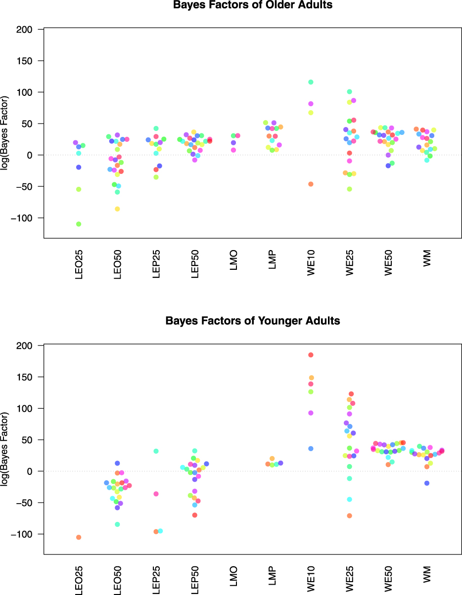
Figure 1. This figure plots the natural logarithm of the aggregate Bayes factors for each model, for each participant for both older adults (top graph) and younger adults (bottom graph). Each color denotes a unique participant. Note if a participant had a Bayes factor of 0 for a given model, the log is undefined and no point is produced. All participants had a Bayes factor of zero for LEP10 and LEO10 and are not plotted here.
Recall our main hypothesis, namely that older adults would obey transitivity at a lower rate than younger adults. Among the 12 models we examined, WM and WE unambiguously capture transitivity, whereas LM and LE permit intransitivity. Participants for whom WM and WE fit poorly may indicate the usage of transitivity-violating decision strategies. Table 3 shows the number of individuals in each group who had a Bayes factor smaller than  ${1 \over 3}$ for WM or WE50 or both in at least one experimental session or stimulus set. These are the number of people for whom a weak order model does not provide a good description of their choices for at least one data set. Older adults generated more violations of weak order models than younger adults.
Table 3. Number (proportion) of participants who violate weak order models in each group

Group-Level Results
We apply the Bayesian test of Cavagnaro and Davis-Stober (Reference Cavagnaro and Davis-Stober2018) to formally test whether older and younger adults differ in their distribution of model classifications. We apply our test to the individual-level Bayes factors aggregated across all six data sets. There were six models that were not selected as a best-fitting model for any participant: LEP25, LEP10, LMO, LEO50, LEO25, and LEO10. We removed these models from consideration for our group-level analysesFootnote 6. The test on the distribution of the six remaining models yielded a Bayes factor of 3.11 in favor of a treatment effect due to age. Table 4 reports the mean posterior distribution estimates of the model classifications for both older and younger adults. These values represent point estimates for the true distribution of model classifications in the older and younger adult populations respectively. Looking at Table 4, older adults are less likely than younger adults to be classified as WE50 (.1 versus .22) or WE10 (.07 versus .22); conversely, older adults are more likely than younger adults to be classified according to LMP (.26 versus .07). The remaining classification probabilities are quite similar between the groups.
Table 4. Mean posterior distribution estimates of model classifications for older and younger adults
The previous test examined the distributions of each of the six models for both groups. We can further refine our hypothesis to focus solely on whether a model was based on weak order or simple lexicographic semiorder preferences. Following Cavagnaro and Davis-Stober (Reference Cavagnaro and Davis-Stober2018), we can aggregate the evidence for similar models and group the remaining Bayes factors according to preferences, ignoring stochastic specification. Table 5 reports the mean posterior estimates for these classifications. Carrying out a test between groups, we find a Bayes factor of 3.49 in favor of a difference between the groups. Table 5 shows that older adults were more likely to be classified according to a simple lexicographic semiorder model (ignoring stochastic specification) than younger adults (mean posterior estimates of .39 versus .12, respectively).
Table 5. Mean posterior distribution estimates of weak order and lexicographic semiorder model classifications for older and younger adults
We can examine in a similar fashion whether the distribution of stochastic specifications in different between older and younger adults. We aggregated evidence for the 6 best-fitting models into two categories: mixture specifications and error specifications. Table 6 reports the mean posterior estimates for these classifications. Older adults were more likely to be classified according to a mixture distribution as compared to younger adults (mean posterior estimates of .47 versus .20). We find a Bayes factor of 2.48 in favor of a difference between the groups.
Table 6. Mean posterior distribution estimates of mixture and error stochastic specifications for older and younger adults
Discussion
We reported the results of a decision making under risk experiment designed to evaluate whether older adults are less likely to obey the axiom of transitivity of preference. We also investigated the nature of possible decision strategy differences between older and younger adults via Bayesian model comparison. The main takeaways from our results are:
• We found relatively weak evidence supporting the hypothesis that older and younger adults used weak order and lexicographic strategies in differing amounts/rates. This conclusion is based on two group-level Bayesian tests that take full account of the classification uncertainty among the various models. It appears that older adults were more likely to be classified according to a lexicographic semiorder model than younger adults, specifically the LMP model.
• A larger portion of older adults showed strong evidence against all weak order based models (all types of stochastic specifications) than younger adults - both in terms of number of individuals as well as number of data sets across experimental sessions and conditions. However, we caution that the absolute number of older adults (4 adults) that consistently displayed weak order model violations was not much greater than the number of younger adults that did so (1 adult).
• We found weak evidence that choices from older adults were more likely than younger adults to be best described via a mixture specification, as compared to an error specification. For fixed preference specifications, older adults were classified to the model with the smallest allowable maximum response error, WE10, at a much smaller rate than younger adults. Consistent with the prior literature on cognitive aging, this suggest that older individuals may be less consistent in their underlying preferences across multiple decisions.
One strength of our study is that our analyses were within-subject in design. This allows us to avoid artifacts due to aggregation (e.g., Estes, Reference Estes1956). We also note that while our models are extremely parsimonious, in that they place strong constraints on the allowable choice probabilities of participants, every data set was classified as best described by a substantive theory. No data set was best described by the encompassing model, suggesting that our models were doing a good job of describing choice behavior. At the same time, the Bayesian analysis focused on a particular collection of 12 models and does not address whether other models could also account for the same data.
It is important to note that there was a large amount of heterogeneity in model classifications for both older and younger adults. This means that there was no “one size fits all” model for either of the two groups. While older adults were more likely to violate weak order models than younger adults, many older adults made choices consistent with weak order based theories, including both types of specifications.
Future work could explore covariates and moderating variables to explain differences in preference structure and choice behavior among older adults. While the current study did not attempt to control for such variables, future work could investigate the role of moderating variables, including neural covariates, measures of cognitive functioning, and health behaviors such as exercise and diet.