2. Numerical method and simulations set-up

Simulations were conducted using a 3-D viscous flow solver where turbulence effects are accounted for via a detached eddy simulation (DES) model. DES is a non-zonal hybrid Reynolds-averaged Navier--Stokes (RANS) – large eddy simulation (LES) method (e.g. see Spalart Reference Spalart2009; Rodi, Constantinescu & Stoesser Reference Rodi, Constantinescu and Stoesser2013) which uses LES away from the solid surfaces. The Spalart-Allmaras (SA) one-equation RANS model was used as the base turbulence model. Near solid boundaries (e.g. channel walls, splitter plate), the distance to the nearest wall d is used to define the turbulence length scale and the original SA, one-equation RANS model is recovered. Away from the solid boundaries, the local grid spacing Δ is used to calculate the turbulence length scale. In these regions, DES reduces to a Smagorinsky-like subgrid-scale model that allows the energy cascade down to the grid size, similar to classical LES. The detached version of the SA DES model was used to improve the accuracy of the predictions. The model solves a transport equation for the modified eddy viscosity, $\tilde{v}$.

A detailed description of the solver and its application to predict shallow flows (e.g. shallow turbulent wakes past cylinders) can be found in Chang, Constantinescu & Tsai (Reference Chang, Constantinescu and Tsai2017) and Zeng & Constantinescu (Reference Zeng and Constantinescu2017). The incompressible Navier–Stokes equations are integrated using a fully implicit, fractional-step method in generalized curvilinear coordinates. An advection–diffusion equation is solved for the non-dimensional concentration of a passive scalar that is used to visualize the coherent structures inside the ML (Constantinescu et al. Reference Constantinescu, Miyawaki, Rhoads and Sukhodolov2016). The convective terms in the momentum equations are discretized using a blend between the fifth-order-accurate, upwind-biased scheme and the second-order, central scheme. All the other terms in the momentum and pressure-Poisson equations are discretized using the second-order, central scheme. The discrete momentum (predictor step) equations and the transport equations for the scalar concentration and $\tilde{v}$ are integrated in pseudo-time using the alternate direction implicit approximate factorization scheme. A double time-stepping algorithm is used to advance the equations in physical time. No wall functions are used in the present implementation of the SA-based DES model. The code is parallelized using multiple passing interface. Validation of the code to predict turbulent flow and mixing in open channels and river confluences is discussed by Keylock, Constantinescu & Hardy (Reference Keylock, Constantinescu and Hardy2012), Constantinescu et al. (Reference Constantinescu, Miyawaki, Rhoads, Sukhodolov and Kirkil2011, Reference Constantinescu, Miyawaki, Rhoads, Sukhodolov and Kirkil2012, Reference Constantinescu, Miyawaki, Rhoads and Sukhodolov2016), Koken, Constantinescu & Blanckaert (Reference Koken, Constantinescu and Blanckaert2013) and Constantinescu (Reference Constantinescu2014). Additional validation of the code to predict dispersion of passive scalars is discussed by Chang, Constantinescu & Park (Reference Chang, Constantinescu and Park2007).

The computational domain is shown in figure 1. The channel bed, the sidewalls and the splitter are modelled as no-slip walls. A convective boundary condition is used at the outlet to allow the coherent structures to leave the computational domain without introducing spurious oscillations in the velocity field (Rodi et al. Reference Rodi, Constantinescu and Stoesser2013). The free surface is modelled as a shear-free rigid lid. This is an acceptable approximation given that the Froude number is less than 0.3 in all simulations. The inlet velocity fields were obtained from preliminary eddy-resolving simulations of periodic, fully developed, turbulent flow in straight channels of same cross-section as that of the inlet sections of the two streams. The non-dimensional concentration of the passive scalar at the tip of the splitter, where the scalar is released, was C = 100. The normal gradient of C was set to be equal to zero at the free surface and the other wall boundaries. At the two inlet boundaries, C was set equal to 0. The molecular Schmidt number was equal to 1.

The characteristic length scale and velocity scale in the non-dimensional simulations were based on the flow depth (D = 67 mm) and (cross-section) mean velocity of the incoming streams at the end of the splitter plate (x = 0), U ₀ = (U ₁₀ + U ₂₀)/2 = 0.23 m s⁻¹, in the base case (H = D, VR = U ₂₀/U ₁₀ = 2.2). The average friction factor of the flow in the incoming streams was ${c_f} = 0.0046$. The magnitude of the mean bed shear stress in the incoming streams can be estimated as ${\tau _0} = 0.5\rho {c_f}U_0^2$, where ρ is the density. This case approximately corresponded to one of the experimental test cases (U ₂₀ = 1.39U ₀, U ₁₀ = 0.61U ₀) discussed by Uijttewaal & Booij (Reference Uijttewaal and Booij2000). The channel width was W = 47D and its length was L_x = 400D (figure 1). The splitter length was 23D. This allows investigating the evolution of the ML over close to 25 m (= 373D), which is more than twice the streamwise distance (x < 11 m) over which measurements were reported in the corresponding experiment and in a preliminary validation simulation performed by Kirkil & Constantinescu (Reference Kirkil and Constantinescu2008). Two more simulations were run. In the H = D/2, VR = 2.2 case, the flow depth was reduced by a factor of 2, while keeping the mean velocities U ₁₀ and U ₂₀ the same. For this simulation, ${c_f} = 0.0052$. Comparison of this test case with the base case allows understanding of the effects of increasing the flow shallowness by reducing the flow depth, which leads to a stronger stabilization effect on the KH billows and thus to a shorter distance over which the ML reaches the quasi-equilibrium regime. In the H = D, VR = 3 case, the velocity ratio was increased, but the mean velocity, U ₀, was kept constant. For this simulation, ${c_f} = 0.0048$. This test case allows understanding of the effects of increasing the initial velocity ratio on the structure and spatial development of a shallow ML.

The mesh contained approximately 16 million cells with 38 grid points distributed over the flow depth. The cell size in the wall normal direction was approximately one wall unit close to the solid boundaries. The mesh was refined near the end of the splitter plate where the KH eddies are generated.

3. Near-field and far-field behaviour of shallow mixing layers

3.1. Spatial development of the ML and dynamics of KH billows

The distributions of the passive scalar concentration in figure 2 show that the ML is always pushed toward the low-speed side. As discussed by Cushman-Roisin & Constantinescu (Reference Cushman-Roisin and Constantinescu2019), this effect is due to the gradual equalization of the velocities in the two streams (i = 1 and i = 2) and can be easily explained using shallow water theory. The streamwise gradient of the Bernoulli function, $U_i^2/2 + gh + gz$, (g is the gravitational acceleration) for each stream is equal to the friction term, $- {c_{fi}}U_i^2$. As the flow depth in the two streams can be considered equal $({h_1}(x) = {h_2}(x))$, the bed elevation, z, is constant and ${U_1}(x) \gt {U_2}(x)$ at all x locations, one can show that the kinetic energy of the faster stream, and thus its velocity, U ₂, decreases monotonically in the streamwise direction, while the opposite is true for the slower stream. Using continuity, this implies that the ML centreline gradually shifts toward the low-speed side until ${U_1}(x) \approx {U_2}(x)$.

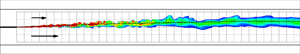
Figure 2. Scalar concentration in the mean and instantaneous flow and non-dimensional turbulent kinetic energy, $k/U_0^2$, near the free surface. (a) H = D, VR = 2.2 case; (b) H = D/2, VR = 2.2 case; (c) H = D, VR = 3.0 case. The dotted line visualizes the ML centreline near the free surface. The non-dimensional concentration of the scalar introduced at the end of the splitter plate is C = 100 but because of strong dilution near the end of the splitter plate much lower maximum values of C are used in the legend to visualize the mixing layer and its coherent structures in the three cases.

The effect of increasing the flow shallowness is to reduce the ML width and the distance over which the ML centreline in the mean flow becomes close to parallel to the streamwise direction. Despite the fact that the initial shear is the same in the H = D and H = D/2, VR = 2.2 cases, bed friction has a larger influence on limiting the growth of the quasi-2-D ML eddies. Pairing of the KH billows is observed until x ≈ 40D (= 80H) in the H = D/2, VR = 2.2 case (figure 2b), compared to x = 150–160D (= 150–160H) in the base case (figure 2a). As pairing of KH billows stops, these quasi-2-D eddies, whose width and length are much larger than the flow depth, rotate less and less around their axes as they are advected downstream. The longitudinal stretching of the cores of these eddies increases and the ML assumes an undulatory shape over the initial stages of the quasi-equilibrium regime. Such a shape was also observed in the experiments (e.g. test case T5) of Chu & Babarutsi (Reference Chu and Babarutsi1988). Figure 3 illustrates the effect of longitudinal stretching on the shape of the KH billows for the base case. The region containing higher concentration fluid around x/D = 250 that corresponds to the core of a quasi-2-D eddy is subject to severe longitudinal stretching. As a result, these eddies gradually lose their coherence. Due to the absence of vortex pairing, the rate of increase of the ML width reduces significantly. The ML undulations are present until the end of the computational domain in the H = D, VR = 2.2 case and their wavelength is about (55–60)D. In the shallower (H = D/2, VR = 2.2) case, the wavelength of the oscillations is close to λ = 24D (= 48H) in the region of highest amplitude. In both cases, the ratio between the wavelength and the locally averaged width of the ML (see § 6) is close to 7.5. The amplitude of the undulations reduces gradually such that the boundaries of the ML become fairly parallel to the streamwise direction around x = 250D (= 500H). For x > 250D, no undulations are observed and the ML width is close to constant. The ML is basically a region containing smaller-scale, energetic eddies generated by the stretching and break-up of the cores of the quasi-2-D eddies. In this region (x > 250D), the ML is in the later stages of the quasi-equilibrium regime.

Figure 3. ML structure near the free surface in the region where the ML assumes an undulatory shape. The ML is visualized using non-dimensional scalar concentration contours in an instantaneous flow field.

Van Prooijen & Uijttewaal (Reference Van Prooijen and Uijttewaal2002) conducted linear-stability analyses for two experimental cases (Uijttewaal & Booij Reference Uijttewaal and Booij2000) and proposed three different regimes in the evolution of the coherent structures. The first case is very similar to the base case in the present paper. For this case, they predicted the growth mode of the dominant mode (wavenumber associated with the maximum energy density representing the largest coherent structures) becomes equal to zero at x ≈ 9.8 m (x/D = 146), which is fairly close to the streamwise location where pairing of the quasi-2-D KH billows ceases in the corresponding simulation (x/D = 150–160). Moreover, their prediction of the length scale of the most unstable mode in the region where the higher-amplitude undulations of the ML are observed in the simulation (3.8 m = 57D at x ≈ 180D ≈ 12 m) is close to the wavelength of the ML undulations (λ = 55–60D) in the region corresponding to the early stages of the quasi-equilibrium regime. These results suggest a link between the first linear-stability regime characterized by a positive growth rate of the dominant mode and the transition regime and also between the second linear-stability regime where the growth rate of the dominant mode is negative while some other modes still have positive growth rates and the early stages of the quasi-equilibrium regime. In the latter regime, the flow is still not stable and the main instability takes the form of undulations on the ML with a wavelength that is roughly equal to 7–8 times the ML width.

The effect of increasing the velocity ratio in the H = D simulations (figure 2a,c) is to generate a faster growth of the ML width and to increase the streamwise distance at which merging of the quasi-2-D eddies stops (e.g. from 160D for VR = 2.2 to 180D for VR = 3). In both cases, the KH billows acquire rapidly an ellipsoidal shape. The width of the largest billows is about 10D for VR = 2.2 and 14D for VR = 3.0. The larger size of the KH billows at a given x location in the H = D, VR = 3.0 case is expected because the rate of growth of the KH instabilities is proportional to the mean shear across the ML, which increases with VR. The same is true for the rate of entrained fluid into the ML which controls the growth of the ML thickness. Larger quasi-2-D eddies will also be able to travel a longer distance before their coherence is destroyed and the ML reaches the quasi-equilibrium regime. For x > 250D, the ML starts interacting with the left bank in the H = D, VR = 3.0 simulation. This is why results for this case will be generally analysed only for x/D < 250.

Another important features of shallow MLs is that the width of the ML is larger near the free surface compared to near the bed over most of the transition regime (figure 4). Although close to the ML origin the interfaces between the ML and the two streams are close to vertical, the interface on the slow-stream side starts tilting during the initial stages of the transition regime. The tilt is the largest around the location where the merging of the quasi-2-D eddies stops. Meanwhile, the tilt of the interface on the high-speed side remains small at all locations. In the base case, the maximum difference between the ML width near the bed and near the free surface is close to 2.5H (x/D ≈ 160, figure 4a) based on the scalar concentration fields, while in the shallower case the maximum difference is only approximately 0.8H (x/D = 30–40, figure 4b). As the quasi-2-D eddies start losing their coherence, the tilt reduces (e.g. to less than 0.3H at x/D = 373 in the base case, figure 4a). In the H = D/2, VR = 2.2 case, the two interfaces become again vertical and the concentration is uniformly distributed over the flow depth for x > 300D.

Figure 4. Non-dimensional scalar concentration in the mean flow in several cross-sections. (a) x/D = 164 and x/D = 373 for the H = D, VR = 2.2 case; (b) x/D = 30 and x/D = 164 for the H = D/2, VR = 2.2 case. The high-speed stream is situated on the left side of each panel. The non-dimensional concentration of the scalar introduced at the end of the splitter plate is C = 100.

3.3. Analysis of the components of the total, depth-averaged, lateral momentum flux

Some components of the total depth-averaged momentum flux may be important contributors to the streamwise momentum balance besides the bed-friction term (Rhoads & Sukhodolov Reference Rhoads and Sukhodolov2008). Analysis of the dominant terms in this equation can reveal the main mechanism generating secondary (transverse) flow that is responsible for the redistribution of the streamwise momentum inside the ML and around it. The bed-friction term is generally the only term considered in simplified models of shallow MLs between parallel streams. Modelling of the other important terms in the depth-averaged streamwise momentum equation is required for development of accurate 2-D, depth-averaged models of shallow flows. In turn, this requires quantitative information on the spatial distribution of these terms in canonical configurations.

The main components of the total, depth-averaged lateral momentum flux are the lateral flux by the mean flow $\langle U\rangle \langle V\rangle /U_0^2$, the dispersive flux due to differential advection over the vertical direction $[\langle UV\rangle - \langle U\rangle \langle V\rangle ]/U_0^2$ and the turbulent flux $\left\langle {\overline {u^{\prime}v^{\prime}} } \right\rangle /U_0^2$, where U and V are the time-averaged streamwise and spanwise velocity components, u′ and v′ are the turbulent velocity fluctuations in the streamwise and transverse directions and 〈 〉 represents a depth-averaged variable. The distributions of these components are shown in figure 5 for the three cases. Given that this is a flow where the main velocity component is the streamwise velocity, the magnitudes of the lateral flux by the mean flow and of the lateral dispersive flux correlate with the spanwise velocity magnitude. In all cases, the peak $\langle V\rangle $ values are observed on the high-speed side of the ML centreline, around the region where its lateral shift is the most rapid. The peak value increases with increasing VR and decreasing flow depth. For example, the maximum spanwise velocity is approximately 0.05U ₀ in the H = D, VR = 2.2 case, 0.07U ₀ in the H = D, VR = 3.0 case and 0.08U ₀ in the H = D/2, VR = 2.2 case.

Figure 5. Distribution of depth-averaged lateral momentum fluxes. (a) H = D, VR = 2.2 case; (b) H = D/2, VR = 2.2 case; (c) H = D, VR = 3.0 case. The frames show the lateral momentum flux by the mean flow, $\langle U\rangle \langle V\rangle /U_0^2$, the dispersive lateral momentum flux $[\langle UV\rangle - \langle U\rangle \langle V\rangle ]/U_0^2$ and the turbulent lateral momentum flux $\bigl\langle {\overline {u^{\prime}v^{\prime}} } \bigr\rangle /U_0^2$. The dotted line visualizes the ML centreline near the free surface.

The distributions of the lateral flux by the mean flow are qualitatively similar in the three simulations, with the region of high magnitude values situated almost entirely on the high-speed side of the flow with respect to the ML centreline. For the dispersive flux, the region of maximum amplification is situated primarily on the high-speed side of the ML centreline in the region where the ML curvature is significant. In all simulations, the dispersive flux is approximately one order of magnitude lower than the lateral flux by the mean flow. The main effect of decreasing the flow depth is to increase the width and length of the region of high magnitude of the lateral flux by the mean flow. While this is also true for the width of the region of high dispersive flux, its length decays with decreasing flow depth, consistent with the shortening of the region where the ML width is different near the bed and near the free surface, which is an indicator of strong vertical non-uniformity of the flow.

In the shallowest case, the turbulent flux is fairly small everywhere except for the thin region close to the ML centreline where KH billows are present (x/D < 130). Even inside this region, the turbulent flux is more than one magnitude lower that the dispersive flux. Both the increase in the flow depth and the increase in the velocity ratio act toward increasing the size of the region of high values of the turbulent flux. In fact, in the H = D simulations, the position and size of the region of high turbulent flux are comparable to the one of high dispersion flux, although the turbulent fluxes are roughly 60%–70 % smaller than the dispersive fluxes.

Overall, these results show that the mean flow plays a much larger role than turbulence in lateral momentum transport associated with the spatial development of a shallow ML between parallel streams. The dispersive fluxes are typically of the order of 5%–10 % of the total lateral momentum flux in the region where the curvature of the ML is significant and thus can play an important role in the redistribution of the streamwise momentum with increasing distance from the ML origin and in the generation of secondary flow. In fact, analysis of the mean flow fields in the H = D simulations shows that weak streamwise-oriented cells of secondary flow are present inside the high curvature part of the ML, where also the vertical flow non-uniformity is the largest (e.g. for 10 < x/D < 120 in the base case). Moreover, the fact that the sum of the lateral flux by the mean flow and of the dispersive flux shows large magnitudes mostly over the fast-stream side of the ML centreline is in agreement with measurements performed in the field by Sukhodolov et al. (Reference Sukhodolov, Schnauder and Uijttewaal2010) for a shallow ML developing between parallel streams in a natural river channel. It also supports their finding that the streamwise gradient of the total lateral momentum flux needs to be retained in 1-D shallow water models only in the depth-averaged streamwise momentum equation for the fast stream, where this term is comparable to the friction-generated fluxes of momentum.

4. Mean streamwise velocity profiles

As the ML is pushed toward the low-speed side (figure 2), the velocity of the fast stream, U ₂(x), decreases while that of the slow stream, U ₁(x), increases with downstream distance. For fixed a fixed z/H, the location of the ML centreline is chosen as that where $u(x,y) = \bar{U}(x) = ({U_1}(x) + {U_2}(x))/2$. Figures 2(a) and 2(b) show that the rate of increase of the shift of the ML centreline is larger in the H = D/2, VR = 2.2 case, at least for x/D < 100. This suggests that the velocity equalization process becomes faster as the flow shallowness increases. Simulation results show that the non-dimensional velocity difference $\mathrm{\Delta }{U^\ast } = \mathrm{\Delta }U/\mathrm{\Delta }{U_0} = ({U_2}(x) - {U_1}(x))/({U_{20}} - {U_{10}})$ decays much faster with the downstream distance in the H = D/2, VR = 2.2 case compared to the H = D, VR = 2.2 case. For example, at x/D = 150, $\mathrm{\Delta }{U^\ast } \approx 0.65$ in the base case and $\mathrm{\Delta }{U^\ast } \approx 0.25$ in the shallower case.

Using shallow water theory and some simplifying assumptions (low Froude number, negligible mixing between the two streams, negligible transverse slope of the free surface) Cushman-Roisin & Constantinescu (Reference Cushman-Roisin and Constantinescu2019) have shown that the length scale that controls the equalization of the mean velocities in the two streams takes place over a distance of the order of several times the length scale ${x^\ast } = {c_f}x/H$ which incorporates the effect of bottom friction via the mean friction coefficient, c_f. Moreover, the difference between the square of the mean velocity in the two streams ${(U_2^2 - U_1^2)^\ast } = (U_2^2 - U_1^2)/(U_{20}^2 - U_{10}^2)$ should be equal to ${\textrm{e}^{ - {x^\ast }}}$. Figure 6(a) shows that the three simulations predict very similar variations of ${(U_2^2 - U_1^2)^\ast }$ with x*. The agreement between the numerical predictions and the theoretical model of Cushman-Roisin & Constantinescu (Reference Cushman-Roisin and Constantinescu2019) is quite good away from the ML origin. Having some larger errors close to the ML origin is somewhat expected as x* becomes the physically relevant length scale only after bed friction starts having a significant effect on the development of the ML. Moreover, the ML has a non-zero width at x = 0 due to the boundary layers on the two sides of the splitter plate. The best agreement is observed for the H = D/2, VR = 2.2 case for which the relative difference between the velocity of the two streams is less than 2 % of the initial difference at the end of the computational domain (x/D = 373). Interestingly, the ${\textrm{e}^{ - {x^\ast }}}$ also provides a fairly good fit to the non-dimensional velocity difference, $\mathrm{\Delta }{U^\ast }$ (figure 6b), although the agreement is slightly less good than that observed for ${(U_2^2 - U_1^2)^\ast }$. This is simply because the centreline velocity $\bar{U}(x) = ({U_1}(x) + {U_2}(x))/2$ varies little in the downstream direction. Using this additional assumption, Van Prooijen & Uijttewaal (Reference Van Prooijen and Uijttewaal2002) have already shown that $\mathrm{\Delta }{U^\ast } = {\textrm{e}^{ - {x^\ast }}}$.

Figure 6. Non-dimensional velocity difference between the two streams in a horizontal plane situated close to the free surface (z/H = 0.85). (a) ${(U_2^2 - U_1^2)^\ast }$ vs. x*; (b) $\mathrm{\Delta }{U^\ast }$ vs. ${x^\ast }$. The solid line shows the theoretical solution ${(U_2^2 - U_1^2)^\ast } = {\textrm{e}^{ - {x^\ast }}}$ and $\mathrm{\Delta }{U^\ast } = {\textrm{e}^{ - {x^\ast }}}$.

The non-dimensional mean streamwise velocity profiles in the transverse direction are compared in figure 7 to the self-similar (error function) solution for a free ML and to the experimental measurements of Uijttewaal & Booij (Reference Uijttewaal and Booij2000) at several streamwise locations (0.05 m < x < 11.0 m, z/D = z/H = 0.85). All variables are defined based on their values in the z/D = 0.85 plane, so their dependence on z is omitted in the definitions bellow. The ML centreline is defined as the transverse location where the streamwise velocity gradient, $\partial u(x,y)/\partial y$, is the largest. The transverse shift of the ML centreline is l_cy(x) and the splitter is located at y = 0. At each streamwise location, the lateral coordinate, y − l_cy, is scaled with the ML width, which is defined as $\delta (x) = ({U_2} - {U_1})/{(\partial u/\partial y)_{max}}$.

Figure 7. Comparison of non-dimensional mean streamwise velocity profiles, (u − U ₁)/(U ₂ − U ₁), predicted by DES (solid lines, 0.05 m < x < 20 m, z/H = 0.85) with the experimental data of Uijttewaal & Booij (Reference Uijttewaal and Booij2000) (solid circles, x < 11 m, z/H = 0.85). The velocity profiles are plotted versus the non-dimensional lateral distance, (y − l_cy)/δ. The dashed red line represents the error-function curve corresponding to the self-similar solution for a free ML.

Overall, the numerically predicted profiles of $(u(x,y) - {U_1}(x))/({U_2}(x) - {U_1}(x))$ show close agreement with the self-similar error-function solution and good agreement with the experimental data at all locations, especially if one considers the scatter in the experimental measurements. The transverse velocity gradient over the central part of the ML is slightly larger for the profiles located at 30 < x/D ≤ 112 compared to the one in the error-function solution. As opposed to the experimental data, there is very little scatter of the predicted velocity profiles on the high-speed side of the ML ((y − l_cy)/δ < −0.7) for x/D > 10. Past the end of the transition regime, the velocity profiles at x/D = 164 and x/D = 299 are very close to the error-function solution. Although not included in figure 7, it is relevant to mention that the non-dimensional velocity profiles for the shallower (H = D/2, VR = 2.2) case are even closer to the error-function solution and show less scatter near the edges of the ML for x/D > 30. So, past the end of the transition regime, the non-dimensional velocity distribution across a shallow ML is very close to that expected in a free ML.

5. Mixing layer shift

The plots of l_cy/H vs. x/H for z/D = 0.85 in figure 8(a) confirm the trends observed in figure 2 showing that the effect of decreasing the flow depth or increasing VR is to increase l_cy. When non-dimensionalized with the flow depth, l_cy increases much more rapidly in the shallower case. Meanwhile, the base case predictions of l_cy/H are in good agreement with the values inferred from the experimental data for x/D < 160. Close to the origin, the increase of l_cy with x is close to linear for all cases. However, the rate of increase of l_cy/H decreases significantly after the end of the transition regime. This is the most evident for the H = D/2, VR = 2.2 case, where the rate of growth of l_cy/H is very small during the later stages of the quasi-equilibrium regime (x/H > 600).

Figure 8. Shift of the ML centreline near the free surface (z/H = 0.85). (a) l_cy/H vs x/D, (b) ${l^{\prime}_{cy}} = {l_{cy}}/D(\Delta U(0)/\bar{U}(0))$ vs x*; (c) $l_{cy}^\ast = {l_{cy}}/D(\Delta U(x)/\bar{U}(x))$ vs x* in log-log scale. Also shown in (a) are the experimental results of Uijttewaal & Booij (Reference Uijttewaal and Booij2000).

Uijttewaal & Booij (Reference Uijttewaal and Booij2000) found that for cases with different flow depths but approximately the same VR, l_cy is mainly a function of x*. Given that VR is not the same in all our simulations, a better way to non-dimensionalize the centreline shift is ${l^{\prime}_{cy}} = {l_{cy}}/D(\Delta U(0)/\bar{U}(0))$. The width of the channel, W, is a more relevant length scale, but given that W/D was kept constant in all simulations, using D instead of W does not change the analysis. The plots in figure 8(b) show that the downstream variation of ${l^{\prime}_{cy}}$ is fairly similar in the three cases. The main reason for this is that $\mathrm{\Delta }{U^\ast } = \mathrm{\Delta }U/\mathrm{\Delta }{U_0}$ is mainly a function of x* (figure 6b). If mixing between the two streams is neglected and the flow depth in the two streams is assumed to be the same, then the widths of the two streams, W ₁ and W ₂, and thus l_cy = (W ₂ − W ₁)/2, are basically a function of ΔU at any given streamwise location (Cushman-Roisin & Constantinescu Reference Cushman-Roisin and Constantinescu2019). So, the flow depth is expected to have a fairly small influence on ${l^{\prime}_{cy}}({x^\ast })$ except indirectly as x* ~ 1/c_f and c_f is a function of the channel Reynolds number that is proportional to H.

A physically more correct way to non-dimensionalize the centreline shift is to include the local values of the velocity in the two streams. This leads to defining a new non-dimensional centreline shift, $l_{cy}^\ast = {l_{cy}}/D(\Delta U(x)/\bar{U}(x))$. This way, the mean shear acting on the ML at a given streamwise location enters the non-dimensionalization of l_cy. As for large x*, the velocity difference $\Delta U$ decays asymptotically to zero (§ 4), $l_{cy}^\ast $ is expected to increase with increasing x*. This is confirmed by results in figure 8(c) that show $l_{cy}^\ast $ vs. x* in log–log scale. Several regions over which $l_{cy}^\ast{\sim} {x^{{\ast}^{\beta} }}$ can be identified. Close to the origin of the ML, a first region with β = 1 is present. Starting at the end of the transition regime (x* ≈ 0.7 for H = D, VR = 2.2 case, x* ≈ 0.9 for H = D, VR = 3.0 case and x* ≈ 0.4 for H = D/2, VR = 2.2 case), a second region with β = 5/3 is present in all three simulations. This region basically corresponds to the early stages of the quasi-equilibrium regime when the ML assumes an undulatory shape. Finally, after all the large eddies lost their coherence and the boundaries of the ML are close to vertical in the instantaneous flow fields (e.g. for x > 250D or x* > 2.5 for the H = D/2, VR = 2.2 case), a region with β = 3 is observed up to x* = 4.

6. Mixing layer width

The reduction in the rate of growth of $\delta $ with the streamwise distance is only partially explained by the reduction in the mean shear across the ML, which is proportional to $\mathrm{\Delta }U(x)$. The extra dissipation due to the no-slip boundary condition at the channel bed also contributes to decay of the coherence of the KH billows and thus to a reduction of δ(x) with respect to a free mixing layer. The streamwise variation of δ(x) near the free surface (z/D = 0.85) is shown in figure 9(a). For the base case, the agreement with the experimental results of Uijttewaal & Booij (Reference Uijttewaal and Booij2000) is very good over the whole region where experimental data are available (x/H < 160). The decrease in δ with decreasing flow depth is due to the increased effect of the bed friction on the dynamics of the KH billows. In the H = D/2, VR = 2.2 case, the ML continues to grow at a much reduced rate during the later stages of the quasi-equilibrium regime (x > 400H or x > 200D) and approaches a constant value by the end of the domain.

Figure 9. Mixing layer width near the free surface (z/H = 0.85). (a) δ/H vs. x/H; (b) ${\delta ^\ast } = {c_f}\delta /H(\Delta U(x)/\bar{U}(x))$ vs. x* in linear scale; (c) ${\delta ^\ast }$ vs. x* in log–log scale. Also shown in (a) are the experimental results of Uijttewaal & Booij (Reference Uijttewaal and Booij2000). The two lines in (c) show best fit, power-law curves for x* < 1.5 and x* > 2. The solid lines in (a) show ML width predictions using the equation proposed by Van Prooijen & Uijttewaal (Reference Van Prooijen and Uijttewaal2002), $\delta (x/H)/H = \alpha (\Delta U(0)/\bar{U}(0))(1/{c_f})(1 - {\textrm{e}^{ - {x^\ast }}}) + \delta (0)/H$. The horizontal dotted lines in (a) show the equilibrium values (x, x*→∞) predicted by the same equation.

As already discussed in § 3.1 based on the mean scalar concentration fields, the ML width close to the free surface is larger than near the bed over part of the ML. Comparison of the plots of $\delta (x) = ({U_2} - {U_1})/{(\partial u/\partial y)_{max}}$ near the free surface (z/D = 0.85) and near the bed (z/D = 0.35) for the base case (figure 9a) shows that these differences develop once bed friction starts affecting the dynamics of the KH billows and peak at the end of the transition regime where the difference is about 1.2H, which corresponds to more than 10 % of the depth-averaged ML width. Then, the difference between the ML width near the free surface and near the bed decreases monotonically in the downstream direction, such that the ML width in the mean flow is close to constant over the flow depth at the start of the quasi-equilibrium regime. Data for the H = D/2, VR = 2.2 case confirm that the ML width does not vary with the distance from the bed during the quasi-equilibrium regime. At the end of the transition regime (x = 40D = 80H), the difference between δ(x) near the bed and bear the free surface is less than 2 % of the depth-averaged ML width.

Using the local velocity in the two streams and the flow depth, one can define a non-dimensional ML width ${\delta ^\ast }(x) = {c_f}\delta /H(\Delta U(x)/\bar{U}(x))$. A similar variable, $S = {\delta ^\ast }/2$ was already introduced by Alavian & Chu (Reference Alavian and Chu1985) and is referred to as the bed-friction number. It characterizes the stabilizing influence of the bottom friction on the development of the ML. Note that ${\delta ^\ast }$ increases in the downstream direction due to the increase in δ and the decrease in ΔU with increasing x or x* (figures 6b and 9a). When plotted against x*, the ${\delta ^\ast }$ curves for the three cases are very close to each other (figure 9b). Moreover, if ${\delta ^\ast }({x^\ast })$ is plotted in log–log scale (figure 9c), one can identify two power-law regions up to x* = 4. The first one corresponds to the transition and initial stages of the quasi-equilibrium regime and is characterized by a linear increase of ${\delta ^\ast }$ with x*. This is formally similar to what is observed for a free shear layer for which $\Delta U(x)$ and $\bar{U}(x)$ are constant. Moreover, the predicted rate of increase $\textrm{d}{\delta ^\ast }/\textrm{d}{x^\ast } = 0.09$ is within the range expected for a free mixing layer. After the end of the initial stages of the quasi-equilibrium regime, a region with ${\delta ^\ast }\sim {x^{{\ast ^3}}}$ (or using some simplifying assumptions $\delta \sim {x^{{\ast ^3}}}{\textrm{e}^{ - {x^\ast }}}$) is present. This does not mean that the ML width growth faster. Figure 9(a) clearly shows that the increase of the ML width with x is very small for x/H > 400 or x* > 2. The presence of regions where ${\delta ^\ast }\sim {x^{{\ast ^n}}}$ with n > 0 simply means that the rate of growth of δ does not decay as e^−x* which is a good approximation to describe the streamwise decay of $\Delta U({x^\ast })$ over the whole length of the shallow ML (figure 6b). In the H = D/2, VR = 2.2 case, the ${\delta ^\ast }\sim {x^{{\ast ^3}}}$ region lasts until α approaches zero (e.g. α < 0.003 for x* > 3) and the mixing layer width reaches a close to constant value.

7. Entrainment coefficient

To describe in a more quantitative way the effects of the bottom friction on the spatial development of a shallow ML, an entrainment coefficient α is defined (Chu & Babarutsi Reference Chu and Babarutsi1988; Uijttewaal & Booij Reference Uijttewaal and Booij2000):

(7.1)\begin{equation}\alpha = \frac{1}{{\Delta U}}\frac{{\textrm{d}\delta }}{{\textrm{d}t}}\sim \frac{{U(x)}}{{\Delta U(x)}}\frac{{\textrm{d}\delta (x)}}{{\textrm{d}x}}.\end{equation}

Its variation can be related to that of the bed-friction number, S, which accounts for the effect of flow shallowness on the evolution of the ML. In the empirical relation proposed by Chu & Babarutsi (Reference Chu and Babarutsi1988), a linear decay of α with S was assumed in between the origin of the ML and the location where the ML transitions to an equilibrium regime where the ML width is constant (e.g. α = 0):

(7.2)\begin{equation}\alpha = {\alpha _0}(1 - S/{S_c}),\end{equation}

where α ₀ is the entrainment coefficient at the ML origin and S_c in the definition given by Chu & Babarutsi (Reference Chu and Babarutsi1988) is the critical value of S corresponding to the transition to the equilibrium (zero-growth) regime (α = 0 based on (7.2)) when production and dissipation of kinetic energy are in equilibrium. Uijttewaal & Booij (Reference Uijttewaal and Booij2000) interpreted the bed-friction number as a measure of the ratio between the dissipation and production of the kinetic energy of the large ML eddies, where the dissipation is driven by bed friction acting on the quasi-2-D eddies while production is driven by the transverse mean shear across the ML. Experiments and stability analysis suggest 0.06 < S_c < 0.12 (Alavian & Chu Reference Alavian and Chu1985; Chu & Babarutsi Reference Chu and Babarutsi1988; Chu et al. Reference Chu, Wu and Khayat1991; Chen & Jirka Reference Chen and Jirka1998; Uijttewaal & Booij Reference Uijttewaal and Booij2000). More recently, Van Prooijen & Uijttewaal (Reference Van Prooijen and Uijttewaal2002) showed that S_c is not a useful number to characterize the large-scale motion because the dominant mode inside the mixing layer starts decaying (e.g. largest coherent structures are losing energy) well before the position where the most unstable mode starts decaying, meaning S = S_c. Given that any shallow ML is expected to behave like a free mixing layer close to its origin, one expects α ₀ ≈ 0.085 − 0.1 (e.g. see Townsend Reference Townsend1956; Pope Reference Pope2000).

The availability of data on δ(x) over the quasi-equilibrium regime in the H = D/2, VR = 2.2 case allows us to gain a more complete picture of the dependence of α with x* and S in the far field of a shallow ML. Results in figures 10(a) and 10(b) show that α and S decay monotonically and approach zero in the far field, consistent with the observed tendency of δ/H in figure 9(a) to approach a zero rate of growth for x/H > 400 (x* ≈ 2). The decay of α with x* is also consistent with the observed effects of the bottom friction that first induces a decay in the rate of growth of the quasi-2-D ML eddies compared to those forming in a free shear layer, then impedes vortex pairing and induces the gradual loss of coherence of these eddies such that the ML region is depleted of large-scale eddies past the early stages of the quasi-equilibrium regime. Even for the base case, simulation results show a monotonic decay of α with the distance from the origin of the ML such that $\alpha \approx 0.01 \ll {\alpha _0}$ by the end of the computational domain (x/D = 400). Predictions of δ(x) using the equation proposed by Van Prooijen & Uijttewaal (Reference Van Prooijen and Uijttewaal2002) were also included in figure 10(a). The model accounts for the exponential decay of ΔU* with x* and assumes the entrainment coefficient to be constant and equal to the value for a free shear layer (e.g. α = 0.085). In the H = D, VR = 2.2 case, the model successfully predicts δ(x) over the transition regime (x < 160H = 10.7 m) but overpredicts δ(x) at larger x/H. The model's predictions are also very accurate in the H = D/2 VR = 2.2 case up to the end of the transition regime (x = 80H) but then start to slowly diverge from the numerical results. Obviously, the predictive capabilities of the model can be improved if a more realistic variation is adopted for the entrainment coefficient. Rather than assuming it to be a constant (e.g. α = 0.085 or α = α ₀), one can propose α = α (x*) or α = α (S) based on the predicted variations of these variables in figures 10(a) and 10(b). In particular, numerical results show a faster monotonic decay of α with x* and S over the transition and early stages of the quasi-equilibrium regime and a slower monotonic decay of α with x* and S over the later stages of the quasi-equilibrium regime where α < 0.005.

Figure 10. Entrainment coefficient, α, as a function of x* (a) and the bed-friction number S (b,c) near the free surface (z/H = 0.85) for the H = D/2, VR = 2.2 case. Also shown in (d) are the estimations of α vs. S based on the experimental results of Uijttewaal & Booij (Reference Uijttewaal and Booij2000) for x < 11 m and based on simulation results for the H = D and $H = D/2$ cases. The dashed lines in (b) show best fit curves, α ~ e^−γS, with γ = 14.7 for S < 0.15 and γ = 3.3 for S > 0.15. These curves are visualized as straight lines in log–linear scale in (c). The solid straight lines in (b,d) correspond to the initial quasi-linear decay of α with S.

Figure 10(b) shows that the decay of α with S for the H = D/2, VR = 2.2 case is not linear except for small values of S and the rate of decay of α with S decreases suddenly for S > 0.15. Figure 9(b) shows that S ≈ 0.15 (e.g. ${\delta ^\ast } \approx 0.3$) when x* ≈ 2, in other words at the location downstream of which the ML is not subject to undulations in horizontal planes. When plotting the data from figure 10(b) in in log–linear scale, one can see that the variation of α with S is close to exponential for both S < 0.15 and S > 0.15 (figure 10c). Over the transition and early stages of the quasi-equilibrium regime where the ML assumes an undulatory shape α = 0.07e^−14.7S, while during the later stages of the quasi-equilibrium regime α = 0.0066e^−3.3S. These two curves also are represented in figure 10(b) and fit quite well the numerical data over the whole channel length. In the limit of S going to zero, the exponential decay function reduces to α = 0.07*(1 − 14.7S) = 0.07(1 − S/0.068) giving α ₀ = 0.07 and S_c = 0.068. This linear best fit curve is also plotted in figure 10(b).

Figure 10(d) shows that for all cases the decay of α with S is close to linear for small values of S, although the values of α ₀ and S_c may vary. For the base case, the linear best fit to the simulation data gives α ₀ = 0.115 and S_c = 0.065. These values are fairly close to the ones inferred from the corresponding experiment, α ₀ = 0.11 and S_c = 0.08. For the H = D, VR = 3.0 case, the linear decay region is characterized by α ₀ = 0.12 and S_c = 0.095 and is observed until the location where the ML starts interacting with the lateral wall of the channel. Chu & Babarutsi (Reference Chu and Babarutsi1988) determined S_c = 0.09 based on their experiments. Simulation data in figure 10 show that the maximum value of S up to which a linear decay of α with S can be assumed is S ≈ 0.04 $({\delta ^\ast } \approx 0.08)$ in the H = D, VR = 2.2 case and S ≈ 0.025 $({\delta ^\ast } \approx 0.05)$ in the H = D/2, VR = 2.2 case. These two values of S correspond to x* ≈ 0.7 and x* ≈ 0.25, respectively. The two x* values are very close to the ones corresponding to the end of the transition regime in the two cases (x* ≈ 0.7 and x* ≈ 0.4). So, the linear empirical relationship of Chu & Babarutsi (Reference Chu and Babarutsi1988) is valid in between the ML origin and the end of the region where the main mechanism for the growth of the ML is pairing of the KH billows. However, an exponential decay law allows characterizing the variation of α with S way beyond the location where vortex pairing ends, basically until the region where the KH billows are destroyed.

8. Dynamics of the Kelvin–Helmholtz billows and large-scale undulatory motions

8.1. Velocity power spectra

Power spectra of the spanwise velocity fluctuations are analysed in the z/H = 0.85 plane at points situated close to the ML centreline. In the base case (figure 11a) the peak of the power density occurs at f = 0.38 Hz (f is the frequency) for x = 2 m (x/D = 30) and at f = 0.09 Hz for x = 11 m (x/D = 164). As the transition regime ends at x/D ≈ 160, each peak corresponds to the passage frequency of the KH billows at that location. These values are in good agreement with those measured in the corresponding experiment (f = 0.35 Hz and f = 0.1 Hz). The streamwise decay in the peak frequency values over the transition regime is related to vortex pairing. Animations show that, on average, one to two vortex merging events take place as the KH billows travel between these two streamwise locations. After the quasi-equilibrium regime starts, the peak frequency remains approximately constant f ≈ 0.06 Hz (e.g. see power spectra at x/D = 299 and x/D = 373). This frequency is associated with the undulatory motions of the ML (figures 2a and 3) that are observed until the end of the computational domain in the base case.

Figure 11. Power spectra of the spanwise velocity fluctuations at points situated close to the centreline of the ML and the free surface (z/H = 0.85). (a) H = D, VR = 2.2 case; (b) H = D/2, VR = 2.2 case; (c) H = D, VR = 3.0 case.

Another feature of the velocity power spectra in figure 11(a) is the presence of a −3 energy decay subrange on the high frequency side of the peak frequency. Measured velocity spectra in the experiment of Uijttewaal & Booij (Reference Uijttewaal and Booij2000) show a similar behaviour for x/D < 165. A −3 subrange was also present in the velocity spectra measured by Vowinckel, Schnauder & Sukhodolov (Reference Vowinckel, Schnauder, Sukhodolov and Cowen2007) in a shallow ML forming at a natural river confluence between two nearly parallel streams. As vortex pairing stops and the quasi-2-D eddies start losing their coherence, the −3 subrange is still present for some distance. The presence of a −3 subrange indicates that the large eddies are quasi-two-dimensional (Batchelor Reference Batchelor1969). The broader −3 energy decay subrange observed at x/D = 299 indicates increased dissipation of the quasi-2-D eddies as they lose their coherence (Vorobieff, Rivera & Ecke Reference Vorobieff, Rivera and Ecke1999). The decrease in the energy associated with the f = 0.06 Hz frequency between x/D = 299 and x/D = 375 is consistent with the decrease in the amplitude of the mixing layer oscillations is the downstream direction.

In the H = D/2, VR = 2.2 case (figure 11b), the last pairing event takes place around x/D = 30, which explains the presence of two peaks in the power density at f = 0.58 Hz and f = 0.27 Hz. The KH billows did not lose their coherence by x/D = 90 where a first peak is present at f = 0.27 Hz. The second peak at f ≈ 0.11 Hz corresponds to the start of the undulatory motions of the ML. By x/D = 164, the coherence of the KH billows is lost and the peak (f = 0.11 Hz) corresponds to that of the undulatory motions. The undulatory oscillations practically disappear for x/D > 250 in the instantaneous flow fields (figure 2b). Consistent with this, the energy of the undulatory motions decays by close to one decade between x/D = 223 and x/D = 299. A main difference with the base case is that the −3 subrange is replaced by a −4.3 subrange. Although the frequency of the ML undulations increases with decreasing flow depth, the corresponding Strouhal number is close in both cases (St = f H/U ₀ = 0.015 − 0.016).

Comparison of figures 11(a) and 11(c) shows that increasing VR while keeping the flow depth constant has only a mild influence on the dominant frequencies observed in the velocity power spectra during the transition regime and the early stages of the quasi-equilibrium regime. The passage frequency of the KH billows increases by about 10 % while that of the ML undulations decreases by 10%–15 %.

8.2. Autocorrelation function of the spanwise velocity fluctuations

The autocorrelation function of the spanwise (v) velocity fluctuations is defined as:

(8.1)\begin{equation}{R_{vv}}(\Delta t) = \frac{\langle {v^{\prime}({t_0}) \cdot v^{\prime}({t_0} + \Delta t)}\rangle }{{{{(\langle v{^{\prime^2}}({t_0})\rangle \langle v{^{\prime^2}}({t_0} + \Delta t)\rangle)}^{0.5}}}},\end{equation}

where the brackets 〈 〉 denote averaging over all values of the time ${t_0}$ and Δt is the time difference. The autocorrelation function is plotted in figure 12 for three points situated along the ML centreline at x/D = 30, 164 and 299 (x = 2, 11 and 20 m) in the z/H = 0.85 plane. At all locations, R_vv is characterized by large-scale oscillations. The time interval between the origin, where R_vv(0) = 1, and the first maximum of R_vv can be interpreted as the passage time of the largest eddies at that location.

Figure 12. Autocorrelation function of the spanwise velocity fluctuations, R_vv. (a) x/D = 36 and x/D = 164; (b) x/D = 299. The autocorrelation function is evaluated close to the ML centreline and the free surface (z/H = 0.85). Also plotted in (a) is the autocorrelation function for the base case from the experiment of Uijttewaal & Booij (Reference Uijttewaal and Booij2000). The vertical lines denote the location of the first maximum of R_vv in the H = D, VR = 2.2 case (solid lines) and H = D/2, VR = 2.2 case (dashed lines).

For the base case, the overall level of agreement with the autocorrelation function estimated from the experiment (x/D = 30, 164) is reasonable. For x/D = 30, the first minimum in the R_vv curve is reached after 1200 ms (x/D = 30) and 5000 ms (x/D = 164) in the simulation and after 1400 ms (x/D = 30) and 4500 ms (x/D = 164) in the experiment (figure 12a). The predicted passage time of the KH billows at x/D = 30 and 164 is approximately 2500 ms and 9700 ms, respectively. These values are consistent with the peak frequencies in the velocity spectra in figure 11(a). Assuming the average velocity of the coherent structures is $\bar{U}(x)$, one can estimate the average streamwise size of the KH billows, or, more precisely the average distance between the centres of two successive billows. This estimated length is approximately 8.2D at x/D = 36 and 31.3D at x/D = 164. At these two locations, δ = 2.7D and 8.8D respectively (figure 9a). Assuming that the spanwise size of the KH billows is close to the ML width, this means that the KH billows are not circular but rather ellipsoidal and their aspect ratio increases as one moves downstream (e.g. from approximately 3 at x/D = 30 to 3.5 at x/D = 164). As vortex pairing ceases around x/D = 164 and the KH billows are stretched mostly along the streamwise direction, the aspect ratio increases rapidly to become close to 5.8 at x/D = 223. At x/D = 299, the first maximum in the autocorrelation function occurs after 17 300 ms, which corresponds to a frequency f = 0.057 Hz, very close to the one associated with the ML undulations in the velocity power spectra (f ≈ 0.06 in figure 11a). The estimated wavelength of the ML undulations is λ = 63D = 63H at x = 299D and λ = 65D at x = 374D. The ratio λ/δ is close to 6.8 for x/D ≥ 299. Qualitatively, the R_vv curves in the H = D, VR = 3 case and the dynamics of the KH billows is similar to that predicted in the base case. The shape factor of the KH billows during the transition regime is close to 3.7, while λ/δ ≈ 7 during the early stages of the quasi-equilibrium regime.

In the H = D/2, VR = 2.2 case, the time of passage of the KH billows at x/D = 30, where vortex pairing is still observed, is approximately 1900 ms, which is approximately 21 % smaller than the value predicted for the base case (2400 ms) at the same location. As for the base case, the shape of the autocorrelation function changes dramatically once the ML transitions to the early stages of the quasi-equilibrium regime. The small attenuation of the amplitude of the R_vv oscillations at x/D = 164 means that the undulatory motions are strongly correlated. The decay in the amplitude of the R_vv oscillations at x/D = 299 is consistent with the observed decay in the amplitude of the undulatory motions. These motions are hardly detectable in the concentration contours for x/D > 250 (figure 2b). The first peak of R_vv occurs after 8000 ms at x/D = 164 and after 8500 ms at x/D = 299, confirming that the wavelength of these undulatory motions varies little (λ ≈ 31D = 62H) as they gradually disappear during the later stages of the quasi-equilibrium regime. Over the region where the undulations are detected in the autocorrelation function, the ratio λ/δ is close to 8.5.

9. Bed shear stress

Consistent with the streamwise decay of the velocity difference between the two streams, the mean bed shear stress, $\bar{\tau }/{\tau _0}$ (${\tau _0}$ is the mean bed shear in the two incoming streams), follows a similar evolution, as illustrated in figure 13 for the base case. Although the ML is a region where the $\bar{\tau }/{\tau _0}$ values are in between those predicted beneath the fast stream and the slow stream, this does not automatically mean that, in the case of a loose bed, most of the sediment is going to be entrained by the fast stream. Cheng, Koken & Constantinescu (Reference Cheng, Koken and Constantinescu2018) have shown that the presence of large-scale coherent structures near the bed can result in a significant amplification of the flux of entrained sediment provided that the time of passage of these eddies over a certain location is sufficiently large to result in sediment entrainment. This is because the entrainment flux is a nonlinear function of the difference between the local bed shear stress and the critical value for sediment entrainment. For flows in which large-scale coherent structures are present near the bed, one should analyse the sediment entrainment capacity of the flow based on the instantaneous bed shear stress distributions, $\tau $, rather than the mean bed shear stress, $\bar{\tau }$. Figure 13(a) illustrates the differences between the distributions of $\bar{\tau }/{\tau _0}$ and $\tau /{\tau _0}$ for the base case. Several elongated regions of high bed shear stress are present in the instantaneous fields inside and close to the ML. Inside these regions, $\tau /{\tau _0}$ is comparable to $\bar{\tau }/{\tau _0}$ beneath the fast stream in the incoming channel.

Figure 13. Distribution of the normalized bed shear stress. (a) $\bar{\tau }/{\tau _0}$, mean flow H = D, VR = 2.2 case; (b) root mean square of the bed shear stress fluctuations, ${\tau ^{rms}}/{\tau _0}$, H = D, VR = 2.2 case; (c) $\tau /{\tau _0}$, instantaneous flow, H = D, VR = 2.2 case; (d) $\tau /{\tau _0}$, instantaneous flow, H = D/2, VR = 2.2 case; (e) $\tau /{\tau _0}$, instantaneous flow, H = D, VR = 3.0 case. Also shown in (f) is the instantaneous streamwise velocity distribution, u/U ₀, and 2-D streamline patterns in the x/D = 122 cross-section for the H = D, VR = 3.0 case. The dotted line visualizes the ML centreline near the free surface. The black and blue arrows point toward patches of large bed shear stress induced by the KH billows and by streamwise cells of secondary flow, respectively. The x/D = 122 cross-section shown in (f) cuts through the elongated streak of high $\tau /{\tau _0}$ situated between x/D = −1 and x/D = 0.3 in (e). The streamwise cell of secondary flow pushes high velocity fluid toward the bed, which induces the formation of a region of high $\tau /{\tau _0}$.

One way to approximate the effect of the bed shear stress amplification induced by the coherent structures and near-bed turbulent fluctuations is to consider the root mean square of the bed shear stress fluctuations. Several investigations have shown that using $\bar{\tau } + C{\tau _{rms}}$ with a value of the empirical constant C around 1 as an effective bed shear stress in sediment entrainment formulas results in more accurate predictions of the sediment entrainment capacity of the flow (Sumer et al. Reference Sumer, Chua, Cheng and Fredsøe2003; Kraft, Wang & Oberlack Reference Kraft, Wang and Oberlack2011; Cheng et al. Reference Cheng, Koken and Constantinescu2018). For the shallow ML flows investigated here, the main types of coherent structures interacting with the channel bed are KH billows and streamwise oriented cells of secondary flow developing inside the ML or close to its boundaries in the instantaneous flow fields. These eddies control the position and shape of the regions of high ${\tau _{rms}}/{\tau _0}$. For example, in the base case the peak ${\tau _{rms}}/{\tau _0}$values are approximately 0.2–0.25 and such large values are observed until x/D = 120, which proves that coherent structures can significantly enhance the capacity of the flow to entrain sediment. The region of high ${\tau _{rms}}/{\tau _0}$ approximately corresponds to the ML position near the bed until x/D ≈ 50. Over this region, the passage of the KH billows controls the large-scale temporal variations of $\tau$. Downstream of this location, most of the region of high ${\tau _{rms}}/{\tau _0}$ is situated on the high-speed side of the ML centreline. Although the cores of the KH billows can still induce a noticeable increase in the instantaneous bed shear stress until x/D ≈ 150, most of the amplification of ${\tau _{rms}}/{\tau _0}$ in this region is due to streamwise-oriented cells of secondary flow.

Though these cells form on both sides of the ML centreline (e.g. see $\tau /{\tau _0}$ distributions for the H = D, VR = 2.2 and H = D, VR = 3 cases in figure 13), the cells on the high-speed side induce the largest τ values. Each cell pushes higher-streamwise-velocity fluid closer to the bed on the side where the vertical velocity induced by the cell is oriented toward the bed. As a result, the bed shear stress increases above its value in the mean flow. Given that $\bar{\tau }/{\tau _0}$ is larger on the high-speed side, so is $\tau /{\tau _0}$. Comparison of the distributions of $\tau /{\tau _0}$ in figures 13(a) and 13(c) shows that the effect of increasing VR is to generate larger streaks of high bed shear stress. Such streaks are observed until x/D = 200 in the H = D, VR = 3.0 case. Figure 13(c) also shows the streamwise velocity distribution and 2-D streamlines patterns in the x/D = 122 cross-section cutting through one of the largest elongated streaks of high $\tau /{\tau _0}$. The streak is induced by the cell whose axis is situated at y/D = −1.5. The region where fluid with higher streamwise velocity is advected toward the bed, −1 < y/D < 0, corresponds to the streak of high $\tau /{\tau _0}$.

The effect of reducing the flow depth from H = D (figure 13a) to H = D/2 (figure 13b) is a weakening of the capacity of the KH billows to induce regions of high $\tau /{\tau _0}$. Such regions are observed only for x/D < 40 in the H = D/2, VR = 2.2 case. However, the most important difference with the H = D simulations is the absence of regions of high bed-friction velocity amplification due to the formation of streamwise cells of secondary flow. Even if such cells sometimes form in the instantaneous flow fields, they are very weak and their effect on the redistribution of the streamwise momentum in the cross-section is relatively low compared to the deeper (H = D) cases. So for very shallow conditions, coherent structures contribute relatively little to the increase of the sediment entrainment capacity of the flow (the peak values of ${\tau _{rms}}/{\tau _0}$ are close to 0.02) and the instantaneous bed shear stress decays fairly monotonically from the high-speed side of the channel to its low-speed side. Consistent with the decrease in the mean velocity difference between the two streams to less than 4 % for x/D > 300, the distribution of the bed shear stress in figure 13(b) is fairly uniform close to the downstream end of the channel.

10. Summary and conclusions

The large length of the channel in the numerical simulations allowed us to analyse the physics of shallow mixing layers forming between parallel streams past the transition regime which was the focus of previous experimental studies. In the shallower H = D/2, VR = 2.2 case, the channel was sufficiently long to allow studying the evolution of a ML until the difference between the mean velocities of the two streams becomes very small $\mathrm{(\Delta }U/\mathrm{\Delta }{U_0} \lt 0.03)$.

Over the transition regime, where the dynamics of the KH billows is strongly affected by bed friction but merging between neighbouring billows is still taking place, the numerical model predictions of the non-dimensional streamwise velocity profiles across the ML, the frequency of passage and aspect ratio of the KH billows, the ML centreline shift and the ML width were in good agreement with data available from experiments. Simulation results showed that the ML increases its vertical non-uniformity during the transition regime. This generates strong dispersive lateral momentum fluxes and secondary flow. The boundary of the ML on the slow-stream side becomes tilted with respect to the vertical, such that the ML width near the free surface is larger than near the bed. The largest difference is observed at the end of the transition regime. In the base case, this difference attains 15 % of the average ML width. The degree of vertical non-uniformity of the flow decreases with increasing flow shallowness. As expected, the largest values of the TKE are induced in the regions where the KH billows are the most coherent. Moreover, the passage of the KH billows and the generation of streamwise cells of secondary flow in the region where the ML is in the transition regime induce regions of high instantaneous bed shear stress especially on the fast-stream side of the ML centreline. For the deeper (H = D) cases, simulation results show that the erosive capacity of the flow will peak inside the ML or in its immediate vicinity rather than beneath the faster stream. There erosion mechanisms are responsible for the formation of the confluence scour hole at low angle natural river confluences.

During the early stages of the quasi-equilibrium regime, the stabilizing effect of bottom friction becomes dominant compared to the destabilizing effect of the mean shear across the ML. The KH, quasi-2-D billows lose their capacity to rotate around their axes and undergo severe stretching in the streamwise direction. Their stretching and gradual loss of coherence is accompanied by a change in the structure of the ML that assumes an undulatory shape and a reduction in the degree of vertical non-uniformity of the ML. In the later stages of the quasi-equilibrium regime, after the quasi-2-D billows lost their coherence, the amplitude of the undulatory motions is very small, the ML boundaries become vertical, and the lateral momentum fluxes by the mean flow and the dispersive lateral momentum fluxes are negligible. Moreover, the transverse profiles of the non-dimensional mean streamwise velocity approaches the error-function profile corresponding to the theoretical solution for a free ML. Although the frequency, f, and wavelength, λ, of the undulatory motions are a function of the flow depth, H, the corresponding Strouhal number is close to constant (St = f H/U ₀ = 0.015 − 0.016). The effect of increasing the velocity ratio, VR, is to increase λ and to decrease f. The ratio λ/δ varies between 7 and 8.5, with the larger values observed in the shallower case.

For all cases, the predicted non-dimensional difference of the square velocities in the two streams is fairly independent of VR and H when represented as a function of the length scale ${x^\ast } = {c_f}x/H$ which incorporates the effect of bottom friction. Consistent with the theoretical model of Cushman-Roisin & Constantinescu (Reference Cushman-Roisin and Constantinescu2019), away from the ML origin, the decay is close to ${\textrm{e}^{ - {x^\ast }}}$ for all cases. Moreover, in a good approximation, the non-dimensional velocity difference, $\mathrm{\Delta }U/\mathrm{\Delta }{U_0} \approx {\textrm{e}^{ - {x^\ast }}}$, a result that can be predicted if one assumes $\bar{U}(x)$ is constant (see also Van Prooijen & Uijttewaal Reference Van Prooijen and Uijttewaal2002). This result is the main reason why the lateral shift of the ML centreline is not a strong function of the flow depth and VR when non-dimensionalized with $\Delta U(0)/\bar{U}(0)$ and a (constant) length scale that is not proportional to the flow depth H. When both the ML width and the centreline shift are non-dimensionalized with the local velocities in the two streams (${\delta ^\ast } = {c_f}\delta /H(\Delta U(x)/\bar{U}(x))$, $l_{cy}^\ast = {l_{cy}}/D(\Delta U(x)/\bar{U}(x))$, several regions can be identified. In particular, simulation results show that ${\delta ^\ast } = 0.09{x^\ast }$ over the transition and early stages of the quasi-equilibrium regime and $l_{cy}^\ast{\sim} {x^\ast }$ over the transition regime. These linear relationships are formally similar to those observed in a free ML but they apply way after bed-friction effects on the evolution of the shallow ML become important.

Consistent with the gradual loss in the coherence of the quasi-2-D KH billows and thus of the capacity of the ML to entrain surrounding fluid, simulation results show that the entrainment coefficient α decays monotonically with increasing x* and increasing bed-friction number S. In the H = D/2, VR = 2.2 case, α ≈ 0 (α < 0.003) for x* > 3 which means that the ML basically reaches the zero-growth regime. The decay of α with S is exponential (α ~ e^−γS), but the value of γ is smaller for S > 0.15, corresponding to the later stages of the quasi-linear regime. During the transition regime, the linear decay relationship assumed by the empirical model of Chu & Babarutsi (Reference Chu and Babarutsi1988) corresponds to the tangent to the exponential decay function at S = 0.

Simulation results also show that approximating the effect of dispersion fluxes in 2-D depth-averaged numerical models of flows containing shallow MLs is even more important than modelling the turbulent fluxes. Numerical data from fully 3-D, eddy-resolving simulations can be used to test some of the modelling hypotheses in analytical models that need to account in an approximate way for the effects of lateral fluxes on the streamwise momentum (e.g. Rhoads & Sukhodolov Reference Rhoads and Sukhodolov2008; Sukhodolov, Schnauder & Uijttewaal Reference Sukhodolov, Schnauder and Uijttewaal2010) and to better understand how mean flow and turbulence affect lateral momentum transfer.