


1. Introduction
It is well known that aerofoil noise can be split into several different types (Brooks, Pope & Marcolini Reference Brooks, Pope and Marcolini1989). Among the various types of aerofoil noise, Fink (Reference Fink1975) investigated the tonal noise generated due to laminar-to-turbulent boundary-layer transition. They showed the existence of a law predicting the tone frequencies from the boundary-layer instability theory. Meanwhile, Paterson et al. (Reference Paterson, Vogt, Fink and Munch1973) observed that the tone frequencies scaled proportionally to the 3/2 power of the free-stream velocity. A feedback loop theory was introduced by Tam (Reference Tam1974). They inferred that the feedback loop took place between the aerofoil trailing edge and a location in the wake. However, this theory was challenged by Longhouse (Reference Longhouse1977), who suggested that the feedback loop occurred between the acoustic waves radiating from the trailing edge and the Tollmien–Schlichting (T–S) instability waves developing in the transition region. Arbey & Bataille (Reference Arbey and Bataille1983) confirmed Paterson's work and suggested that the tones were predicted using the following formula:
 \begin{equation} \frac{f_nL_c}{a_{\infty}} = \frac{U_c/a_{\infty}}{L/L_c}\left(n+\frac{1}{2}\right)\left(1+\frac{U_c/a_{\infty}}{1-M_{\infty}}\right)^{-1}, \end{equation}
where f n is the modal frequency,  $a_{\infty }$ is the speed of sound,
  $L_c$ is the aerofoil chord length,
  $U_c$ is the convection speed of the boundary layer,
  $M_{\infty } = U_{\infty }/a_{\infty }$ is the free-stream Mach number,
  $L$ is the distance separating the feedback locations and
  $n$ is an integer. The equation, which is a modified version of the earlier one introduced by Tam (Reference Tam1974), clarifies that the feedback loop takes place between the trailing edge and the transitional region. Acoustic pressure waves scattered by the trailing edge propagate upstream at the speed of sound and trigger T–S instabilities in the transition region which will further generate hydrodynamic disturbances convecting downstream within the boundary layer at convection speed
  $U_c$. The incoming hydrodynamic waves are then radiated by the trailing edge and the process reiterates at a discrete frequency. This fixed frequency depends on the speed of sound, the convection speed and the distance separating the transitional region from the trailing edge.
Nash, Lowson & McAlpine (Reference Nash, Lowson and McAlpine1999) and McAlpine, Nash & Lowson (Reference McAlpine, Nash and Lowson1999) discussed the modelling of tonal noise in the case of a separating laminar boundary layer in the vicinity of the trailing edge. Their results were further confirmed by Tam & Ju (Reference Tam and Ju2012) in a direct numerical simulation. After many experimental investigations, Desquesnes, Terracol & Sagaut (Reference Desquesnes, Terracol and Sagaut2007) performed a direct numerical simulation to study tonal noise mechanisms and inferred that secondary discrete frequencies are created due to a bifurcation of the aerofoil wake from a symmetric to an asymmetric vortex pattern. Jones & Sandberg (Reference Jones and Sandberg2011) showed that the tonal contribution becomes less significant compared to the broadband noise at high angles of attack. Arcondoulis et al. (Reference Arcondoulis, Doolan, Zander and Brooks2013) used formula (1.1) and found a satisfying agreement between the theory and their experimental observations. Chong, Joseph & Kingan (Reference Chong, Joseph and Kingan2013) experimentally studied the tonal noise of a NACA0012 aerofoil for various angles of attack and Reynolds numbers. They found that the most effective tonal noise requires the T–S waves to be amplified by a separated boundary layer near the trailing edge. This was further supported by Pröbsting, Serpieri & Scarano (Reference Pröbsting, Serpieri and Scarano2014) and Pröbsting, Scarano & Morris (Reference Pröbsting, Scarano and Morris2015) from their particle image velocimetry measurements in the same range of Reynolds numbers and angles of attack. Nguyen et al. (Reference Nguyen, Golubev, Mankbadi, Yakhina, Roger, Pasiliao and Visbal2017) distinguished the vortex shedding frequency from the acoustic feedback loop frequency.
An additional study on controlled-diffusion aerofoil was investigated by Padois et al. (Reference Padois, Laffay, Idier and Moreau2016) and Sanjose et al. (Reference Sanjose, Jaiswal, Moreau, Towne, Lele and Mann2017). The latter emphasised quiet and intense time strands where the quiet period is driven by attached boundary layers and the intense period involves an unstable separation bubble. To summarise, coherent T–S instabilities coupled with the presence of a recirculation bubble in the vicinity of the trailing edge is the most effective condition for generating an aerofoil tonal noise.
An efficient method to decrease the aerofoil tonal noise would be of interest to many. The authors, however, have not identified various methods in this regard except the modified trailing edge (TE) studied by Chong & Joseph (Reference Chong and Joseph2013). They tested four different sawtooth serration geometries fitted to a NACA0012 aerofoil. They did observe a reduction of the tonal noise when the serrated TEs were used, compared to an unmodified TE. They suggested that the reduction might be related to an abatement of the two-dimensionality in the T–S waves near the TE leading to a decorrelated T–S amplification. They also hypothesised that the serrated TE would be more effective if the separation bubble is located closer to the TE.
Following the work of Chong & Joseph (Reference Chong and Joseph2013), the main objective of this paper is to clarify the hypothesis of the tonal noise reduction due to the serrated TE. For this purpose, the authors use a high-fidelity numerical simulation to provide detailed flow and acoustic information. The noise reduction mechanisms found in this paper are twofold: (i) the presence of a serrated TE diminishes the amplitude of the acoustic source pressure in the transitional region which lowers the acoustic source at the TE and (ii) there is an elevated level of destructive phase interference in the acoustic source when a serrated TE is used.
2. Computational details
This section aims to introduce the governing equations, numerical methods and computational set-up of the present study. The current numerical investigation utilises a high-resolution implicit large-eddy simulation (LES) approach based on a wavenumber-optimised discrete filter. The filter acts as an implicit subgrid scale (SGS) model that dissipates scales smaller than the filter cutoff. It has been demonstrated by Garmann, Visbal & Orkwis (Reference Garmann, Visbal and Orkwis2013) and many others that an implicit LES is capable of capturing flow physics as accurately as the conventional SGS model based LES.
2.1. Governing equations and numerical schemes
The present numerical study is based on a wall-resolved LES by using the three-dimensional compressible Navier–Stokes equations. The Navier–Stokes equations (with a source term for the sponge layer implementation) can be written in a conservative form, transformed onto a generalised coordinate system as
 \begin{equation} \frac{\partial}{\partial t}\left(\frac{\boldsymbol{Q}}{J}\right)+ \frac{\partial}{\partial\xi_i}\left(\frac{\boldsymbol{E}_j-Re^{-1}_\infty M_\infty\boldsymbol{F}_j}{J}\frac{\partial\xi_i}{\partial x_j}\right)=-\frac{a_\infty}{L_c}\frac{\boldsymbol{S}}{J}, \end{equation}
where the indices  $i=1,2,3$ and
  $j=1,2,3$ denote the three dimensions and
  $a_\infty$ is the ambient speed of sound. The vectors of the conservative variables, inviscid and viscous fluxes are given by
 \begin{equation} \left.\begin{gathered} \boldsymbol{Q}=[\rho,\rho u,\rho v,\rho w,\rho e_{t}]^\textrm{T},\\ \boldsymbol{E}_j=[\rho u_j,(\rho uu_j+\delta_{1j}p),(\rho vu_j+\delta_{2j}p),(\rho wu_j+\delta_{3j}p),(\rho e_{t}+p)u_j]^\textrm{T},\\ \boldsymbol{F}_j=[0, \tau_{1j}, \tau_{2j}, \tau_{3j}, u_i\tau_{ji}+q_j]^\textrm{T}, \end{gathered}\right\} \end{equation}
with the stress tensor and heat flux vector written as
 \begin{equation} \tau_{ij}=\mu\left(\frac{\partial u_i}{\partial x_j}+\frac{\partial u_j}{\partial x_i}-\frac{2}{3}\delta_{ij}\frac{\partial u_i}{\partial x_i}\right), \quad q_j=\frac{\mu}{(\gamma-1)Pr}\frac{\partial T}{\partial x_j}, \end{equation}
where  $\xi _i=\{\xi ,\eta ,\zeta \}$ are the generalised coordinates,
  $x_j=\{x,y,z\}$ are the Cartesian coordinates,
  $\delta _{ij}$ is the Kronecker delta,
  $u_j=\{u,v,w\}$,
  $e_{t}=p/[(\gamma -1)\rho ]+u_ju_j/2$ and
  $\gamma =1.4$ for air. The local dynamic viscosity
  $\mu$ is calculated by using Sutherland's law (White Reference White1991). In the current set-up,
  $\xi$,
  $\eta$ and
  $\zeta$ are aligned in the streamwise, wall-normal and spanwise directions, respectively. The Jacobian determinant of the coordinate transformation (from Cartesian to generalised) is given by
  $J^{-1}=|\partial (x,y,z)/\partial (\xi ,\eta ,\zeta )|$. In this paper, the free-stream Mach and Reynolds numbers are defined as
  $M_\infty =u_\infty /a_\infty$ and
  $Re_\infty =\rho _\infty u_\infty L_c/\mu _\infty$. The Mach number is fixed at
  $M_\infty =0.4$ and a Reynolds number of
  $Re_\infty =2.5\times 10^{5}$ is considered. The governing equations are non-dimensionalised based on the aerofoil chord length
  $L_c$ for length scales, the ambient speed of sound
  $a_\infty$ for velocities,
  $L_c/a_\infty$ for time scales and
  $\rho _\infty a^{2}_\infty$ for pressure. Temperature, density and dynamic viscosity are normalised by their respective ambient values:
  $T_\infty$,
  $\rho _\infty$ and
  $\mu _\infty$.
The spatial derivatives are calculated by using an optimised pentadiagonal compact finite difference scheme that is globally fourth-order accurate up to the boundaries (Kim Reference Kim2007). A matching fourth-order Runge–Kutta scheme is used for explicit time marching with a Courant–Friedrichs–Lewy number of 1.0. A sixth-order pentadiagonal compact filter with a normalised cutoff wavenumber of 0.85 ${\rm \pi}$ (Kim Reference Kim2010) is used to dissipate unresolved subgrid scales and ensure the numerical stability. The computation is distributed over 512 processor cores based on a message passing interface (MPI) parallelisation. The MPI parallelisation of the compact scheme and filter is implemented by using the quasi-disjoint matrix system proposed by Kim (Reference Kim2013). All simulations are executed on IRIDIS-4 at the University of Southampton.
2.2. Computational domain, grid and boundary conditions
The present simulation is based on a symmetric Joukowski aerofoil with a 12 % thickness. We consider three different TE geometries in this study: baseline (BTE) and two serrated (STE) cases. The conventional sawtooth serrations are used. Grid meshes used in the current work are displayed in figure 1. A structured H-type topology is used in the present grid and the cells are gradually stretched from the aerofoil surface to the far boundaries. In the BTE case, a constant spanwise grid spacing is used. Meanwhile, in the STE cases, a finer grid spacing is used near the sharp corners. The tips and roots of the serrations are gently rounded (with a radius of 3 % of the span) in order to maintain a continuous mesh without losing the sharp character of the serration. The leading edge of the aerofoil is on the  $z$-axis. In the BTE case, the trailing edge lies at
  $(x,y)/L_c=(1,0)$. In the paper, two different STE geometries are considered; STE1 with an aspect ratio of 0.5 and STE2 of 1.0. The aspect ratio is defined by the streamwise length divided by the spanwise wavelength of the serration. The serrations extend from the baseline geometry. The local chord length is the same as the baseline case at the roots of the serrations and it becomes longer at the tips.

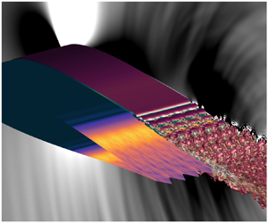
Figure 1. A bird's eye view of the surface mesh for the BTE and STE2 aerofoils (20 % of total cells shown) (a,c) and a cross-sectional view of the interior mesh of the BTE case (25 % of total cells shown) (b).
The spanwise domain size is set to 5 % of the chord length ( $L_z=0.05L_c$) of the baseline aerofoil. This span length is also set as the wavelength of the serrations. The aerofoil chord is aligned with the x-axis. The entire grid consists of
  $N_{\xi } \times N_{\eta } \times N_{\zeta } = 961 \times 481 \times 51 = 23.6$ million points where
  $N_{\xi },N_{\eta }$ and
  $N_{\zeta }$ are the streamwise, vertical and spanwise number of points. The wall-unit grid spacings are presented in figure 2 and they all meet the wall-resolved LES criteria recommended by Georgiadis, Rizzetta & Fureby (Reference Georgiadis, Rizzetta and Fureby2010):
  ${\rm \Delta} s^{+} < 40$,
  ${\rm \Delta} z^{+} < 40$ and
  ${\rm \Delta} n^{+} < 1$ in the turbulent region where
  ${\rm \Delta} s^{+},{\rm \Delta} n^{+}$ and
  ${\rm \Delta} z^{+}$ are the body-fitted streamwise, wall-normal and spanwise wall-unit grid spacings, respectively.

Figure 2. Wall-unit grid spacings used in the BTE case where  ${\rm \Delta} s^{+}$ is the streamwise curvilinear spacing,
  ${\rm \Delta} z^{+}$ is the spanwise spacing and
  ${\rm \Delta} n^{+}$ is the wall-normal spacing.
Characteristics-based non-reflecting boundary conditions (Kim & Lee Reference Kim and Lee2000) are used in the far field boundaries. A sponge layer (Kim, Lau & Sandham Reference Kim, Lau and Sandham2010a,Reference Kim, Lau and Sandhamb) is introduced via the source term  $\boldsymbol {S}$ in (2.1) around the far field boundaries to enforce the damping of acoustic waves and therefore avoid spurious reflections. A no-slip iso-thermal wall boundary condition is applied on the aerofoil surface. A periodic boundary condition is applied across the spanwise boundaries.
Each simulation is run for  $tu_\infty /L_c=16.0$ time units in total where the fully developed solutions are taken during the last 4.0 time units for data processing. In figure 3, time- and spanwise-averaged profiles of the pressure and skin friction coefficients (
 $C_p$ and
  $C_f$) are compared with corresponding XFoil predictions. It is shown that the time-averaged solution matches very well with the XFoil prediction over the laminar region of the flow. There is a noticeable deviation in the turbulent region perhaps attributable to the difference between the two- and three-dimensional approaches.

Figure 3. Time-averaged profiles of the pressure coefficient  $C_p$ and skin friction coefficient
  $C_f$. The BTE profile is spanwise averaged whereas the STE profiles are extracted from the mid-span cross-section. The laminar separation bubble (LSB) range is also depicted.
2.3. Calculation of the acoustic field
For the current study, an established approach originally proposed by Ffowcs–Williams and Hawkings (FW–H) is adopted to calculate the acoustic solutions in the far field. The ‘Formulation 1A’ derived by Farassat (Reference Farassat2007) is implemented in this paper. Since the monopole and quadrupole contributions are irrelevant to the current study, the loading noise is solely considered and the following equation is used:
 \begin{align} 4 {\rm \pi}p'_{L} &= \int_{S} \left[\frac{\dot{p}\cos \theta}{a_{\infty} r (1-M_r)^{2}} + \frac{\hat{r}_i \dot{M}_i p \cos \theta}{a_{\infty} r (1-M_r)^{3}}\right]_{{ret}} \,\mathrm{d} S\nonumber\\ &\quad + \int_{S} \left[\frac{p(\cos \theta - M_i n_i)}{r^{2} (1-M_r)^{2}} + \frac{(M_r - M_{\infty}^{2}) p \cos \theta}{r^{2} (1-M_r)^{3}}\right]_{{ret}} \,\mathrm{d} S, \end{align}
where subscript  $L$ designates the loading noise component; ‘
 $\boldsymbol {\cdot }$’ is the time derivative; ‘ret’ stands for ‘retarded time’;
  $M = {M_1,M_2,M_3};\ M_{\infty } = |\boldsymbol {M}|$ is the Mach number;
  $\hat {\boldsymbol {r}}$ is the unit radiation vector between the source and the observer;
  $r$ is the source–observer distance;
  $\cos \theta = \boldsymbol {n}\boldsymbol {\cdot }\hat {\boldsymbol {r}}$;
  $M_r = \boldsymbol {M}\boldsymbol {\cdot }\hat {\boldsymbol {r}}$; and
  $S$ is the surface of integration. A numerical validation of this implementation can be found in Turner & Kim (Reference Turner and Kim2020). A constant non-dimensionalised radius of 10 is taken for all the presented results and appropriate observer angles are specified later on. Moreover, for the range of frequencies exposed (
 $1<f\kern0.2pt L_c/a_{\infty }<25$),
  $f\kern0.2pt r/a_{\infty }>10$ so the observer truly lies in the far field.
2.4. Definition of variables for statistical analysis
Data processing and analysis are carried out upon the completion of each simulation. The main property required in this study is the power spectral density (PSD) function of pressure fluctuations on the aerofoil surface and at the far field observer location. The pressure fluctuation is defined as
 \begin{equation} p^{\prime}(\boldsymbol{x},t)=p(\boldsymbol{x},t)-\bar{p}(\boldsymbol{x}), \end{equation}
where  $\bar {p}(\boldsymbol {x})$ is the time-averaged pressure. Following Goldstein (Reference Goldstein1976), the one-sided PSD functions of the pressure fluctuations based on frequency are defined by
 \begin{equation} S_{pp}(\boldsymbol{x},f)=\lim_{T\rightarrow\infty}\frac{P(\boldsymbol{x},f,T)P^{*}(\boldsymbol{x},f,T)}{T}, \end{equation}
where  $P$ is an approximate Fourier transform of
  $p^{\prime }$ based on the following definition:
 \begin{equation} P(\boldsymbol{x},f,T)=\int_{-T}^{T}{p^{\prime}(\boldsymbol{x},t)\exp({-2{\rm \pi}\mathrm{i}ft})\,\mathrm{d} t}, \end{equation}
and, ‘ $*$’ denotes a complex conjugate. In the above equations, T represents the half-length of the time signals used for the approximate Fourier transform. The present study also exhibits the wall pressure jump which is defined in the frequency domain by
 \begin{equation} {\rm \Delta} P(\boldsymbol{x},f,T)=\int_{-T}^{T}{{\rm \Delta} p^{\prime}(\boldsymbol{x},t)\exp({-2{\rm \pi}\mathrm{i}ft})\,\mathrm{d} t}, \end{equation}
where  ${\rm \Delta} p^{\prime } = p^{\prime }_u - p^{\prime }_l$ is the difference between the pressure fluctuations on the upper and the lower sides of the aerofoil.
3. Results and discussion
The results of the current study are presented under three subsections. The first part shows how the acoustic feedback loop and the corresponding tonal noise are retrieved from the current LES data. It also depicts how the upstream travelling acoustic wave affects the laminar separation bubble. The second part discusses the tonal noise abatement in the presence of trailing edge serrations. The third part investigates the effect of the spanwise domain length.
3.1. Acoustic feedback loop generating a tonal noise
Figure 4(a) shows some surface contour plots of the wall pressure fluctuations at five different frequencies, obtained from (2.6), for the BTE case. Only the second half of the chord is displayed for clarity. Figure 4(b) shows spanwise-averaged PSDs of the wall pressure fluctuations measured at a few different streamwise locations. The first observation made from figure 4 is that the tonal peak at  $f\kern0.2pt L_c/a_{\infty } \simeq 3.9$, is originated from the local area (
 $x/L_c\simeq 0.72$) where the boundary-layer transition occurs. As indicated earlier, the tonal peak is generated by an acoustic feedback loop which has extensively been investigated by Jones & Sandberg (Reference Jones and Sandberg2011). The present results are compared with the findings of Arbey & Bataille (Reference Arbey and Bataille1983). First, it is necessary to estimate the convection velocity of the tonal component in the turbulent boundary layer. For this purpose, a wavenumber–frequency Fourier transform of the streamwise velocity fluctuation is computed on a mid-span plane along a path line which extends from
  $x/L_c=0.8$ to
  $1.0$ and displaced from the wall by approximately 20 % of the boundary-layer thickness (at the TE). The resulting contour map of the wavenumber–frequency Fourier transform (magnitude) is displayed in figure 5. Based on the data, a least square best fit is performed (as shown in the figure). The best fit gives an estimated convection speed of
  $U_c/a_{\infty } = 0.223$ corresponding to 55.6 % of the free-stream velocity. By using (1.1), a tonal frequency of
  $f\kern0.2pt L_c/a_{\infty } = 3.81$ is predicted for
  $n=3$. This is within only a 2 % deviation from the current LES result, which confirms the presence of an acoustic feedback loop. In the far field noise spectra presented, the contribution of quadrupole sources is considered negligible for two reasons: (i) only the dipole term (surface integral) of the FW–H calculation is used and (ii) at the low free-stream Mach number of the current study, any footprint of the wake noise captured in the surface integral would be substantially weaker than the dipole contribution. Hence, the tonal noise calculated with the FW–H dipole formula may be solely attributed to Arbey & Bataille's feedback model.

Figure 4. (a) Contour maps of the PSD of wall pressure fluctuations (WPF) on the suction side of the BTE case in log scale at five different frequencies, where the black dashed line indicates the transition location; and (b) spanwise-averaged PSDs of WPF on the suction side extracted at four different streamwise locations:  $x_1/L_c = 0.72$,
  $x_2/L_c = 0.80$,
  $x_3/L_c = 0.90$ and
  $x_4/L_c = 0.99$.

Figure 5. A wavenumber–frequency spectrum of the streamwise velocity fluctuation (the magnitude of the Fourier transform) extracted on a mid-span plane along a path-line displaced from the wall by approximately 20 % of the boundary-layer thickness at the TE in the BTE case. Least square best fit line with a slope of  $0.223$ is also displayed.
A more in-depth investigation of the acoustic feedback loop is presented in figure 6. The solid grey contour lines show the upstream travelling acoustic waves (based on pressure fluctuations) at  $f\kern0.2pt L_c/a_{\infty } = 3.9$. Since the acoustic waves are masked by the turbulence in the near field, the authors have extrapolated them (dashed grey) with the following function:
 \begin{equation} \zeta(\boldsymbol{x},t) = \sin\left[2{\rm \pi} f_0 \left(t - \frac{r(\boldsymbol{x})}{u_{ac}}\right)\right], \end{equation}
where  $f_0$ is the tonal frequency,
  $r(\boldsymbol {x})$ is the distance between the TE and the point
  $\boldsymbol {x}$,
  $u_{ac}$ is the acoustic velocity which depends on the flow speed. The vertical cross-stream velocity time derivative fluctuation
  $\textrm {d}v/\textrm {d}t$ emphasises the size variation of the laminar separation bubble canopy illustrated by the pink contour line. The quantity
  $\textrm {d}v/\textrm {d}t$ is filtered at the feedback frequency
  $f\kern0.2pt L_c/a_{\infty } = 3.9$. The filtering is applied by a narrowband window as follows:
 \begin{gather} \widetilde{\frac{\textrm{d}v}{\textrm{d}t}}(\boldsymbol{x},t) = \mathcal{F}^{-1}\left\{W(\,f)\mathcal{F}\left\{\frac{ \textrm{d} v}{\textrm{d} t}(\boldsymbol{x},t)\right\}\right\}, \end{gather}
 \begin{gather}W(\,f) = \sum_{m=0}^{1} \exp [-\alpha (\,f+(-1)^{m} f_0)^{2}], \end{gather}
where  $\mathcal {F}$ and
  $\mathcal {F}^{-1}$ represent the Fourier and inverse Fourier transforms, respectively; ‘
 $\tilde {-}$’ denotes a filtered variable;
  $\alpha$ is a damping parameter (
 $\alpha =5$) and
  $f_0$ is the frequency around which the signal is to be filtered. It can be seen from the plots that a detached LSB is generated when the expansion wave (blue arrow) hits the main LSB. Moreover,
  $\textrm {d} v/\textrm {d} t$ shows in figure 6 an increased magnitude on the edge of the LSB as time marches emphasising the fact that the LSB is excited by the incoming acoustic expansion wave and its tail broadens as the secondary LSB detaches. The incoming acoustic wave front and the LSB canopy are structures from two different scales, therefore a close up of the LSB canopy is proposed in figure 7 along with a velocity vector field visualisation to picture the LSB detachment more accurately. Figure 8 displays the time evolution of the bubble canopy. The time frame is close to the feedback period and the periodic detachment of the secondary LSB is well illustrated by the white dashed lines.

Figure 6. Visualised acoustic feedback loop in a mid-span plane showing flood of filtered vertical cross-stream velocity time derivative fluctuation  $\textrm {d}v/\textrm {d}t$ at
  $f\kern0.2pt L_c/a_{\infty } = 3.9$, contour lines of acoustic wave front (solid grey), extrapolated acoustic wave front in the near field (dashed grey) and the laminar separation bubble canopy (solid pink) in the BTE case.

Figure 7. Close up of the velocity vector field near the LSB detachment in the BTE case. Snapshots are synchronised with the ones in figure 6.

Figure 8. Time evolution of the laminar separation bubble over a period  $(t_8 - t_1)a_{\infty }/L_c=0.28$ in the BTE case. Frames are extracted with a time step of
  $({\rm \Delta} t) a_{\infty }/L_c=0.04$. The white dashed lines depict the periodic detachment of the secondary LSB.
3.2. Influence of serrated trailing edges on the acoustic feedback loop
Instantaneous plots of the generated sound waves are illustrated in figure 9 based on the divergence of velocity  $\partial (u_j/a_{\infty })/\partial (x_j/L_c)$. It should be noted here that the mesh resolution is maintained sufficiently fine for the high-frequency components up to about half a chord length away from the aerofoil surface. Figure 9 compares the BTE, STE1 and STE2 cases. It is noticeable from the figure that the overall intensity of the sound waves becomes weaker as a sharper STE is used, compared to the BTE case.

Figure 9. Contour map of the divergence of velocity  $\partial (u_j/a_{\infty })/\partial (x_j/L_c)$ on a mid-span plane comparing the BTE, STE1 and STE2 cases.
More details of the noise reduction due to the STEs are further investigated in figure 10 where the loading noise from (2.4) is explored. The far field sound pressure fluctuation spectra in figure 10(a) clearly show the tonal noise component at  $f\kern0.2pt L_c/a_\infty =3.9$ in the BTE case, which becomes significantly reduced when the STEs are used. Figure 10(b) presents the relative change of the spectra (due to the use of the STEs) in a decibel scale. It is observed that a 10 dB reduction of the tonal noise is obtained in the STE2 case. Meanwhile, the noise increase observed at lower frequencies might be due to the usage of a reasonably small spanwise domain size – as figure 17 suggests that a longer spanwise domain size tend to lower the peak and shift it towards even lower frequencies – as well as a time signal not sufficiently long to accurately address low-frequency events. Although the magnitudes are captured more accurately by the narrowband spectra in figure 10, figure 11 gives a better insight into the spectrum trend by showing one-third-octave band (a) individual PSDs and (b) sound pressure level (SPL) differences. At higher frequencies, it is relatively clear that STE1 does not produce any broadband noise reduction whereas STE2 performs better with an attenuation of 4 dB compared to BTE at
  $f\kern0.2pt L_c/a_{\infty }=20$. This result is in agreement with the past investigations conducted by Gruber, Joseph & Chong (Reference Gruber, Joseph and Chong2011) on serrations. They demonstrated that significant noise reduction occur above a critical serration aspect ratio of 1.0 (corresponding to STE2 in the present study).

Figure 10. Power spectral density of far field sound pressure fluctuations (loading noise from (2.4)) over a narrow circular arc  $80^{\circ }\le \theta \le 100^{\circ }$ of a radius of
  $r/L_c=10$ centred at the TE of the baseline aerofoil
  $(x/L_c,y/L_c,z/L_c)=(1.0,0,0)$: (a) the individual PSDs and (b) the relative difference of the STE cases to the baseline in decibels.

Figure 11. One-third-octave band power spectral density of far field sound pressure fluctuations (loading noise from (2.4)) over a narrow circular arc  $80^{\circ }\le \theta \le 100^{\circ }$ of a radius of
  $r/L_c=10$ centred at the TE of the baseline aerofoil
  $(x/L_c,y/L_c,z/L_c)=(1.0,0,0)$: (a) the individual PSDs and (b) the relative difference of the STE cases to the baseline in decibels.
Figure 12 shows the acoustic source pressure distribution at the tonal frequency quantified by a Fourier transform of the wall pressure jump between the upper and lower surfaces of the aerofoil (see (2.8)). In this paper, the proposed mechanisms of the tonal noise reduction due to the STEs are twofold: (i) decreased magnitude of the acoustic source pressure in the transitional region (figure 12a) and (ii) incoherent phase distribution of the acoustic source downstream of the transitional region (figure 12b). A reduced intensity of the acoustic source pressure at the transition when the serrated geometries are used results in a reduced intensity of the acoustic source at the TE and consequently means that the acoustic excitation of the transitional separation bubble upstream becomes less effective. The reduced intensity of the acoustic source at the transition in the serrated cases (figure 12a) could be attributed to the laminar separation bubble behaviour in this region. As depicted in figure 8, a secondary LSB detaches from the main LSB with a clear periodic pattern in the BTE case whereas in the STE2 case (figure 13), the secondary LSB re-merges with the main LSB and weaker recirculation is produced. The authors theorise that the merging of LSBs inhibits the secondary LSB detachment and that the absence of LSB detachment may explain the reduced amplitude of acoustic source pressure in the transitional region at the tonal frequency. Figure 14 provides the profiles of the source phase variation (at the tonal frequency) as a function of the spanwise coordinate, obtained at the transition location and at the TE. The reference phase is set to the spanwise-averaged value at the transition location, for each of the three cases. The graphs show that there is a significant phase variation as much as  $180^{\circ }$ in the STE cases whereas the baseline case maintains a highly uniform distribution. This variation is likely to produce some destructive interference and supports the second mechanism proposed in this paper. There exist similar phase interference effects discussed for TE broadband noise (Avallone et al. Reference Avallone, van der Velden, Ragni and Casalino2018) and leading edge interaction noise (Turner & Kim Reference Turner and Kim2019).

Figure 12. Surface contour maps of the Fourier transform of the wall pressure jump at the tonal frequency  $f\kern0.2pt L_c/a_\infty =3.9$: (a) the magnitude in log scale and (b) the phase distribution. The reference phase
  $\phi _{ref}$ is the spanwise-averaged value at the transition location (
 $x/L_c=0.72$).

Figure 13. Time evolution of the laminar separation bubble over a period  $(t_8 - t_1) a_{\infty }/L_c=0.28$ in the STE2 case. Frames are extracted with a time step of
  $({\rm \Delta} t) a_{\infty }/L_c=0.04$.

Figure 14. Spanwise variation of the phase of the wall pressure fluctuations taken at the tonal frequency  $f\kern0.2pt L_c/a_{\infty }=3.9$: (a) at the transition location and (b) along the TE.
3.3. Impact of the spanwise domain length
For completeness of the present study, a span length investigation is also reported below. On top of the three cases BTE, STE1 and STE2 performed with 5 % span (one serration resolved), BTE-ext. and STE2-ext. cases have been run using an extended 10 % span (two serrations resolved). Figures 15 and 16 compare the  $C_p$ and
  $C_f$ profiles obtained with the two different spanwise domain sizes for BTE and STE2 cases. In both cases, the results are very close. Figures 17 and 18 display the FW-H comparison. The integration uses juxtaposed aerofoils. While BTE and STE2 were integrated over
  $0.05L_c\times 401=20.05L_c$ total span length, BTE-ext. and STE2-ext. were integrated over
  $0.1L_c\times 201=20.10L_c$ total span length making the total span lengths comparable. Furthermore, the FW–H calculation is already converged when the span is repeated to
  $20L_c$. BTE and BTE-ext. give a very similar far field sound and it is clear that STE2-ext. provides a clearer trend of noise reduction compared to STE2 at the tonal frequency. The broadband component remains the same at higher frequencies. The exploration of the acoustic source (wall pressure jump) in figure 19(a) explains the above observation: in the 10 % span case, the magnitude of acoustic source pressure in the transitional region is slightly lower than in the 5 % span case. Furthermore, the phase distribution shows more variation along the TE (figure 19b). This phenomenon is emphasised in figure 20 where the phase along the serrated trailing edge is compared between STE2 and STE2-ext. cases. In the 10 % span case, greater variations of the phase are detected. Hence, both mechanisms previously inferred are consistent enough to explain why the extended span case produces a clearer trend of sound attenuation.

Figure 15. Time-averaged profiles of the pressure coefficient  $C_p$ and skin friction coefficient
  $C_f$. The BTE profiles are spanwise averaged.

Figure 16. Time-averaged profiles of the pressure coefficient  $C_p$ and skin friction coefficient
  $C_f$. The STE profiles are extracted at the tip of the serrations.

Figure 17. Power spectral density of far field sound pressure fluctuations (loading noise from (2.4)) over a narrow circular arc  $80^{\circ }\le \theta \le 100^{\circ }$ of a radius of
  $r/L_c=10$ centred at the TE of the baseline aerofoil
  $(x/L_c,y/L_c,z/L_c)=(1.0,0,0)$ comparing two span lengths: (a) the individual PSDs and (b) the relative difference of the STE2 cases to the baseline in decibels.

Figure 18. One-third-octave band power spectral density of far field sound pressure fluctuations (loading noise from (2.4)) over a narrow circular arc  $80^{\circ }\le \theta \le 100^{\circ }$ of a radius of
  $r/L_c=10$ centred at the TE of the baseline aerofoil
  $(x/L_c,y/L_c,z/L_c)=(1.0,0,0)$ comparing two span lengths: (a) the individual PSDs and (b) the relative difference of the STE2 cases to the baseline in decibels.

Figure 19. Comparison of 5 % span (top) and 10 % span (bottom) for STE2 case with surface contour maps of the Fourier transform of the wall pressure jump at the tonal frequency  $f\kern0.2pt L_c/a_\infty =3.9$: (a) the magnitude in log scale and (b) the phase distribution.

Figure 20. Comparison of the spanwise variation of the phase of the wall pressure fluctuations taken at the tonal frequency  $f\kern0.2pt L_c/a_{\infty }=3.9$ along the TE between the STE2 and STE2-ext. cases.
  $L_z=0.1L_c$ and the distribution for STE2 is repeated two times.
4. Conclusions
This paper has investigated how the aerofoil tonal noise could be reduced due to a STE, based on a large-eddy simulation of a Joukowski aerofoil with a 12 % thickness at  $Re_{\infty }=250\,000$,
  $M_{\infty }=0.4$ and zero incidence angle. The current simulation properly captured the well-known acoustic feedback loop and the consequent tonal noise generation. The interaction of the upstream travelling acoustic wave with the laminar separation bubble was studied in detail. It has thus been shown that the incoming acoustic expansion wave directly excites the main LSB, giving birth to detached secondary LSBs at the tonal frequency. Also, the significant reduction of the tonal noise due to the STEs which Chong & Joseph (Reference Chong and Joseph2013) reported, is validated by the current LES results. It has been demonstrated that using a sawtooth STE with a length of 5 % of the chord and an aspect ratio of 1.0 achieved a 10 dB noise reduction of the tonal noise, in the present aerofoil geometry and flow condition used. A secondary investigation reported a comparison of two spanwise domain sizes (5 % and 10 % chord respectively) and it was found that the extended span case gives a clearer trend of noise reduction at the tonal frequency. Two major mechanisms of the tonal noise reduction were suggested in this paper. The first was the reduced intensity of acoustic source pressure (or wall pressure jump) in the transitional region in the presence of STE which directly weakens the scattering at the TE. The second was the early breakdown of the spanwise coherence in the acoustic source which is likely to create destructive interference in the acoustic feedback process. The two inferred mechanisms are also comprehensible in explaining the clearer trend of noise abatement shown by the extended span case.
Acknowledgements
We would like to acknowledge the support of VESTAS for this work, with special thanks to Dr R. Serré, Mr D. Samora Cerqueira and Mr T. Vronsky. We also would like to thank EPSRC for the computational time made available on the UK supercomputing facility ARCHER via the UK Turbulence Consortium (EP/R029326/1), and the local IRIDIS-4 at the University of Southampton. All data supporting this study are openly available from the University of Southampton repository at doi:10.5258/SOTON/D1520.
Declaration of interests
The authors report no conflict of interest.


