


1. Introduction
Lateral gradients of temperature and salinity are omnipresent in the ocean, and thermohaline intrusions and interleaving often occur in these areas (Woods, Onken & Fischer Reference Woods, Onken and Fischer1986; Holbrook et al. Reference Holbrook, Paramo, Pearse and Schmitt2003; Ruddick & Richards Reference Ruddick and Richards2003; Timmermans & Marshall Reference Timmermans and Marshall2020). Thermohaline intrusions are of great importance since they generate fine-scale thermohaline structures, drive lateral flux and mixing and affect the evolution of mesoscale vortices (Merryfield Reference Merryfield2000; Lee & Richards Reference Lee and Richards2004; Ruddick, Oakey & Hebert Reference Ruddick, Oakey and Hebert2010; Sarkar et al. Reference Sarkar, Sheen, Klaeschen, Brearley, Minshull, Berndt, Hobbs and Naveira Garabato2015; Bebieva & Timmermans Reference Bebieva and Timmermans2019; Tang et al. Reference Tang, Tong, Hobbs and Morales Maqueda2019). Numerous studies have been carried out to understand the formation mechanism and transport properties of thermohaline intrusions and interleaving (Ruddick Reference Ruddick2003; Ruddick & Kerr Reference Ruddick and Kerr2003; Krishnamurti Reference Krishnamurti2006). One of the characteristic features of the interleaving is a set of vertically stacked layers with alternating current directions, and double diffusive mixing is believed to be one of the key mechanisms which induces and maintains the layering morphology (Radko Reference Radko2013; Radko & Sisti Reference Radko and Sisti2017).
Double diffusive convection (DDC) happens when the fluid density depends on two scalars which have very different molecular diffusivities and experience certain gradients. The difference in diffusivities of temperature and salinity is usually two orders of magnitude, and the ocean is prone to double diffusive mixing (You Reference You2002). Since the groundbreaking work of Stern (Reference Stern1967), various studies have proved that double diffusive mixing can generate interleaving unstable modes for different frontal configurations, which agree with the field observations in many aspects (Ruddick Reference Ruddick2003; Ruddick & Kerr Reference Ruddick and Kerr2003; Radko Reference Radko2013). The key mechanism is that the double diffusive transport between interleaving layers can further enhance the stratification and the intrusions.
In most of the existing studies, the interleaving and layering usually happen within the water mass body which experiences the vertical and horizontal gradients of temperature and salinity, such as the uniform gradient configuration and heated sidewall configuration, e.g. see Ruddick (Reference Ruddick2003), Krishnamurti (Reference Krishnamurti2006), Simeonov & Stern (Reference Simeonov and Stern2007) and Hebert (Reference Hebert2011), to name a few. In those configurations, intrusion layers develop at the same depth where the scalar gradients are present. Experiments also demonstrated that the intrusion can grow near a cooled sidewall into the regions where the horizontal gradients are not preset (Malki-Epshtein, Phillips & Huppert Reference Malki-Epshtein, Phillips and Huppert2004). Here, by direct numerical simulation (DNS), we reveal that surface gradients in temperature and salinity can generate horizontal gradients in the fluid layer below through double diffusive processes. These gradients subsequently lead to thermohaline interleaving and spontaneous layering. Briefly, surface gradients can be a reason for the development of intrusion underneath.
The rest of the paper is organized as follows. In § 2 we describe the flow configuration, the governing equations and the numerical method. Next, in § 3, we discuss the evolution of flow morphology from the initial field. Then, in § 4, we present analyses concerning the statistically steady state, including the interleaving layers and the horizontal transport properties. Finally, in § 5 we provide the conclusions of the study.
2. The governing equations and numerical method
We consider a Cartesian box with the height  $H$ in the
  $z$-direction and a length
  $L$ in the
  $y$-direction. Gravity is in the negative
  $z$-direction. The flow is statistically homogeneous in the
  $x$-direction. At the top boundary both temperature and salinity increase along the
  $y$-direction with two homogeneous regions at the two ends. Such distributions of two scalars will simultaneously drive the convection flow in the domain. Hereafter, we respectively refer to the
  $(x,y,z)$ directions as the spanwise, streamwise and vertical directions, since the convection motions are mainly in the
  $y-z$-plane, as shown later. An illustrative sketch of the flow configuration is shown in figure 1.

Figure 1. Sketch showing the flow domain with boundary conditions in the  $y$–
$y$– $z$ plane. The two arrows at the two ends inside the domain indicate the direction of the convection cell if the flow is driven only by one of the two scalar gradients.
The fluid density is assumed to be linearly dependent on both temperature and salinity as  $\rho ^{*}=\rho ^{*}_0[ 1-\beta _T T^{*} + \beta _S S^{*} ]$. Here,
  $\rho ^{*}$ is density with
  $\rho ^{*}_0$ being the value at the reference state;
  $T^{*}$ and
  $S^{*}$ are the deviations of temperature and salinity from the reference state, respectively. From now on the asterisk stands for the dimensional quantities. The parameter
  $\beta _T$ is the thermal expansion coefficient;
  $\beta _S$ is the coefficient of the density increase due to salinity change. The Oberbeck–Boussinesq approximation is employed for the governing equations, which read
 $$\begin{gather} \partial_t \boldsymbol{u}^{*} + \boldsymbol{u}^{*} \boldsymbol{\cdot}\boldsymbol{\nabla}\boldsymbol{u}^{*} ={-} \boldsymbol{\nabla} p^{*} + \nu \nabla^{2} \boldsymbol{u}^{*} +g(\beta_T T^{*}-\beta_S S^{*})\boldsymbol{e}_z, \end{gather}$$
 $$\begin{gather}\partial_t T^{*} + \boldsymbol{u}^{*} \boldsymbol{\cdot}\boldsymbol{\nabla} T^{*} = \kappa_T \nabla^{2} T^{*}, \end{gather}$$
 $$\begin{gather}\partial_t S^{*} + \boldsymbol{u}^{*} \boldsymbol{\cdot}\boldsymbol{\nabla} S^{*} = \kappa_S \nabla^{2} S^{*}, \end{gather}$$
 $$\begin{gather}\boldsymbol{\nabla}\boldsymbol{\cdot}\boldsymbol{u}^{*} = 0. \end{gather}$$
Here,  $\boldsymbol {u}^{*}$ is velocity,
  $p^{*}$ is pressure,
  $\nu$ is kinematic viscosity,
  $g$ is the gravitational acceleration and
  $\boldsymbol {e}_z$ is the unit vector in the
  $z$-direction;
  $\kappa _T$ and
  $\kappa _S$ are the two molecular diffusivities. In the first term on the right-hand side of (2.1a) the density has been absorbed into the pressure. We then non-dimensionalize the flow quantities by the free-fall velocity
  $\sqrt {g\beta _T {\rm \Delta} _T H}$, the domain height
  $H$ and the total scalar increments
  ${\rm \Delta} _T$ and
  ${\rm \Delta} _S$ along the top surface, respectively. The non-dimensional form of the governing equations is then
 $$\begin{gather} \partial_t \boldsymbol{u} + \boldsymbol{u} \boldsymbol{\cdot}\boldsymbol{\nabla}\boldsymbol{u} ={-} \boldsymbol{\nabla} p + Pr^{1/2}Ra^{{-}1/2}\nabla^{2} \boldsymbol{u} + (T-\varLambda S)\boldsymbol{e}_z, \end{gather}$$
 $$\begin{gather}\partial_t T + \boldsymbol{u} \boldsymbol{\cdot}\boldsymbol{\nabla} T = Pr^{{-}1/2}Ra^{{-}1/2}\nabla^{2} T, \end{gather}$$
 $$\begin{gather}\partial_t S + \boldsymbol{u} \boldsymbol{\cdot}\boldsymbol{\nabla} S = Pr^{1/2}Ra^{{-}1/2}Sc^{{-}1}\nabla^{2} S, \end{gather}$$
 $$\begin{gather}\boldsymbol{\nabla}\boldsymbol{\cdot}\boldsymbol{u} = 0. \end{gather}$$
The control parameters include the Prandtl number, the Schmidt number, the thermal Rayleigh number and the density ratio, which are defined, respectively, as
 \begin{equation} Pr = \frac{\nu}{\kappa_T},\quad Sc=\frac{\nu}{\kappa_S},\quad Ra=\frac{g\beta_TH^{3}{\rm \Delta}_T}{\nu\kappa_T},\quad \varLambda=\frac{\beta_S{\rm \Delta}_S}{\beta_T{\rm \Delta}_T}. \end{equation}
Note that  $Ra$ measures the strength of the temperature difference;
  $\varLambda$ represents the relative strength of the salinity difference compared with that of temperature difference, i.e. the ratio of the density anomaly induced by the salinity difference to that by the temperature difference. Another important parameter is the aspect ratio of the domain, namely the ratio between the domain length and height
  $\varGamma =L/H$.
In this study the Prandtl number is fixed at  $Pr=7$, and the Schmidt number at
  $Sc=21$. Note that
  $Sc=21$ is much smaller than the typical value in the ocean, of approximately
  $700\sim 1000$. However, large
  $Sc$ requires very fine grids and presents a big challenge for DNS. Therefore, a smaller
  $Sc=21$ is chosen in the present study, which is a common treatment in DDC simulations (Stellmach et al. Reference Stellmach, Traxler, Garaud, Brummell and Radko2011; Paparella & von Hardenberg Reference Paparella and von Hardenberg2012). Here, we set
  $\varLambda =1$ so that the effects of temperature and salinity on the density compensate each other. For different cases we change
  $Ra$ and
  $\varGamma$.
The governing equations (2.2a)–(2.2d) and the continuity equation are numerically solved by our in-house code with the finite-difference and fraction of time step method, which has been extensively used for wall-turbulence and convection flows (Ostilla-Mónico et al. Reference Ostilla-Mónico, Yang, van der Poel, Lohse and Verzicco2015). In the present study the multi-grid method is not used, mainly due to the relatively small Schmidt number  $Sc=21$. The two endwalls in the streamwise direction are imposed by an immersed-boundary technique. The bottom wall and two endwalls in the streamwise direction are no slip for velocity and adiabatic for two scalars. The top surface is free slip and has increasing
  $T$ and
  $S$ along the
  $y$-direction, see the curve in figure 1. At both ends of the top surface, temperature and salinity are uniform over a width of
  $L/8$ with either low or high values. Between the two regions a smooth step function is used for the scalar distribution. In the spanwise direction we fix the width as
  $H$ and use periodic boundary conditions. Initially, the fluid is at rest and with uniform temperature and salinity distributions at
  ${\rm \Delta} T/2$ and
  ${\rm \Delta} S/2$, respectively. Small perturbations are added to both scalar fields to trigger the flow.
The details of the numerical simulations are summarized in table 1. The first three cases are run with fixed aspect ratio  $\varGamma =L/H=4$, and increasing
  $Ra=10^{8}$,
  $10^{9}$ and
  $10^{10}$. For the fourth case we use a larger aspect ratio of
  $\varGamma =8$ and
  $Ra=10^{8}$, in order to investigate the effects of the domain length. As will be shown in the following sections, the evolution of the system has a very large time scale. Therefore, the simulations have to be run for a very long time period. For example, the shortest run here is already over 25 000 non-dimensional time units. This brings up another challenge to the numerics, and only four cases are considered in the present study.
Table 1. Summary of the numerical set-up. Columns from left to right are: case number, Rayleigh number, density ratio, Prandtl number, Schmidt number, the aspect ratio of domain, the resolutions in each direction, the total simulation time and the time period during which the statistics are sampled.

3. Development of the interleaving
We present, in this section, how the flow motions develop from the initial field and lead to the interleaving layering. Since the two endwalls and the bottom boundary are adiabatic, the total heat and salinity fluxes over the top surface should be around zero once the flow reaches the statistically steady state. Figure 2 displays the time history of these fluxes over the entire simulation of case 1, where the fluxes are measured by the Nusselt number  $Nu_\zeta ^{top} = (- \kappa _\zeta \partial _z \langle \zeta \rangle _{top})/ (\kappa _\zeta {\rm \Delta} _\zeta {H}^{-1})$ with
  $\zeta =T$ or
  $S$. Here,
  $\langle \cdot \rangle _{top}$ denotes the spatial average over the top boundary. For the time period
  $t<3000$, the system undergoes a strong transition stage. Starting from
  $t\approx 3000$, oscillations emerge in the time history of the fluxes. After
  $t\approx 9000$, the fluxes oscillate with a stable period around
  $3000$. This suggests that the dominant flow structures have a relatively large characteristic time scale.

Figure 2. Time evolution of the total heat and salinity fluxes, measured by two Nusselt numbers  $Nu^{top}_T$ and
  $Nu^{top}_S$, over the top boundary for case 1.
The flow structures which induce the oscillations in the total fluxes are interleaving layers. In figure 3 we show the instantaneous fields of temperature, salinity and streamwise velocity on the spanwise mid-plane at four different times for case 1. Initially, both scalars have uniform distributions equal to the corresponding mean values over the top boundary. Then, just below the left half of the top boundary, the temperature and salinity differences favour the diffusive type of DDC. While on the right half, the fingering type of DDC develops. This initial stage can be seen in the top row of figure 3, where the flow structures on left and right parts have distinct horizontal scales. The different types of DDC beneath the top boundary transport heat and salinity with different rates at the two opposite sides of the domain, which sets up horizontal scalar gradients within the domain. Then interleaving layering emerges from the left side and extends horizontally towards the right side, as shown from the second to the bottom row in figure 3. Once established, these interleaving layers are the dominant structures in the flow and exhibit a complex dynamics, which will be discussed in detail in the next section.

Figure 3. The development of the flow field for case 1. Rows from top to bottom are for the times  $500, 1500, 3000, 9000$, and columns from left to right show the fields of temperature, salinity and streamwise velocity in the spanwise mid-plane, respectively.
The different types of DDC can be illustrated by the density ratio defined by the vertical temperature and salinity gradients. Stability theory suggests that the fluid layer is unstable to the diffusive oscillatory instability when  $1>\varLambda _z>(Pr+\tau )/(Pr+1)=0.917$ (Veronis Reference Veronis1965), and to the salt-finger instability when
  $1<\varLambda _z<1/\tau =3$ (Stern Reference Stern1960), respectively. Here,
  $\tau =\kappa _S/\kappa _T=1/3$ is the diffusivity ratio between two components. In figure 4 we plot the local density ratio
  $\varLambda _z=(\beta _T\partial _zT)/(\beta _S\partial _zS)$ for the flow fields shown in figure 3. We highlight in the left column the region that is highly susceptible to diffusive DDC, and in the right column the region in favour of fingering DDC. Initially, both diffusive and fingering regimes are scattered throughout the domain and then the two types concentrate on the opposite sides. Note that the interleaving mainly occurs on the left part, see the bottom right panel in figure 3. The intrusion is of the diffusive type with layers sloping down to the cold and fresh side (Stern Reference Stern2003). When the flow reaches the statistically stable state, both diffusive and salt-finger interfaces can be identified. These interfaces exist between the velocity interleaving layers, which we will discuss in detail in the next section.

Figure 4. The evolution of the vertical density ratio  $\varLambda _z$ for case 1. Rows from top to bottom are for the times
  $500, 1500, 3000, 9000$, and left and right columns show the DDC type in diffusive and fingering regimes, respectively.
4. Interleaving structures and horizontal transport
As shown in the previous section, once the interleaving layers are fully developed, they occupy the majority of the flow domain. The total fluxes through the top boundary exhibit long-time-period oscillations. In this section, we focus on the fully developed stage of the flow, and discuss the dynamics and transport properties of the layers. We summarize in table 2 all the key statistics from the numerical simulations, which will be discussed in detail in the following subsections.
Table 2. Summary of the numerical results. Columns from left to right are as follows: case number, layer thickness, the maximal current velocity, the upward-shifting velocity of the layer, Nusselt numbers for temperature and salinity, Reynolds number, the horizontal density flux ratio and the isohaline slope.

4.1. Flow structures of interleaving
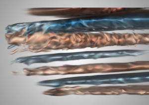
We first show the detailed flow structures for case 2 in figures 5(a) and 5(b) by the three-dimensional volume rendering of the streamwise and vertical velocities. A stack of interleaving layers is distinctively observed in the domain. For this case seven layers are visible. The layers extend upward towards the positive streamwise direction and have alternating flow directions with a positive or negative streamwise velocity, which is a clear indication of interleaving. The layers have long horizontal length and relatively small vertical thickness. In figure 5(c) we plot the profiles of the temperature and salinity anomalies at seven different streamwise locations. Here, the anomaly of scalar  $\zeta$ is calculated as
  $\zeta '=\bar {\zeta }-\overline {\bar {\zeta }}$. Hereafter, one bar stands for the spanwise average, and two bars for the spanwise and temporal average. Coherent temperature and salinity anomalies exist along the interleaving currents.

Figure 5. Thermohaline interleaving for case 2 at  $t=35\,000$ depicted by the volume renderings of (a) the streamwise velocity and (b) the vertical velocity, in which the positive
  $y$-direction is from left to right. (c) The profiles from left to right are for temperature anomaly (red dashed line) and salinity anomaly (blue solid lines) at
  $y=iL/8$, with
  $i=1\cdots 7$.
Once the flow reaches the steady quasi-periodic state, the mean temperature and salinity fields drive different types of flows within the domain. To demonstrate this, we plot in figure 6(a) the contours of spanwise and temporally averaged temperature and salinity fields. At the upper left and upper right corners, the isotherms and isohalines are almost horizontal and parallel. The gradients of both scalars are mainly in the vertical direction, and DDC occurs with the diffusive type near the left corner and the fingering type near the right corner. The fingering DDC generates the small-scale vertical motions on the right in figure 5(b). At the left part of the bulk region, where the layering is the strongest, the isotherms and isohalines have different inclination angles. By averaging over the main intrusion region, as marked by the dashed rectangular in figure 6(a), the mean inclination angle for isotherms is approximately  $25^{\circ }$ and that for isohalines is approximately
  $11^{\circ }$. The interleaving currents have an inclination angle of approximately
  $3^{\circ }$, which is smaller than those of the isotherms and isohalines, a phenomenon consistent with the intrusion theory (Ruddick Reference Ruddick2003; Radko Reference Radko2013).

Figure 6. (a) Contours of spanwise and temporally averaged temperature  $\overline {\bar {T}}$ (solid lines) and salinity
  $\overline {\bar {S}}$ (dashed lines). (b) Flow regions susceptible to different types of double diffusion. Colours represent the Turner angle
  $Tu$, with blue colours indicating the diffusive type and red colours the fingering type, respectively. Here,
  $Tu$ is calculated by the spanwise averaged scalar gradients
  $\partial _z\bar {T}$ and
  $\partial _z\bar {S}$ for the flow field shown in figure 5.
The different types of DDC can be also identified by the Turner angle, which is defined by the vertical gradients of the mean scalars as  $Tu=135^{\circ }-\arg (\beta _S \partial _z \bar {S} + i\beta _T \partial _z \bar {T})$ (Ruddick Reference Ruddick1983). Here,
  $i$ is the imaginary unit, and
  $\arg$ stands for the argument of the imaginary number. Fingering DDC usually happens in the range
  $45^{\circ }< Tu<90^{\circ }$, and diffusive DDC in the range
  $270^{\circ }< Tu<315^{\circ }$. In figure 6(b) we present the distribution of
  $Tu$ for the flow field shown in figure 5, where the mean gradients are calculated after spanwise averaging. Again, both fingering and diffusive DDC exist in the flow field. The region with
  $45^{\circ }< Tu<90^{\circ }$ agrees with the vertical motions in figure 5(b), namely, those vertical motions are mainly fingering convection. At the upper-right corner, the fingering DDC is driven by the vertical salinity and temperature gradients imposed by the top boundary. In the left part of the bulk, the layers with fingering DDC correspond to the interfaces below the leftward moving currents with higher temperature and salinity and above the rightward moving ones with lower temperature and salinity. Meanwhile, diffusive DDC dominates the upper left region, where
  $270^{\circ }< Tu<315^{\circ }$. The layers with
  $270^{\circ }< Tu<315^{\circ }$ correspond to the interfaces above the leftward moving warm and salty currents and below the rightward moving cold and fresh ones. Different types of DDC between interleaving currents are characteristic phenomena of thermohaline intrusion (Ruddick Reference Ruddick2003; Radko Reference Radko2013).
4.2. The upward shift of the layers
Moreover, our numerical results reveal that the vertical location of each layer is not constant. Rather, these layers shift upward over a very large time scale, which is clearly shown in supplementary movie 1 available at https://doi.org/10.1017/jfm.2021.753. Figure 7 displays the time evolution of the vertical profiles of streamwise velocity at location  $y=3/8L$, i.e. where the interleaving currents are strongest. For case 2, it takes approximately
  $10\,000$ non-dimensional time units for one layer to move from the bottom to the top surface. Detailed investigation indicates that the total density difference between the two ends in the streamwise direction periodically changes sign, and close to the bottom boundary new layers are generated accordingly with alternating movement directions.

Figure 7. The upward shifting of the interleaving layers depicted by the time evolution of the spanwise-averaged profiles of the streamwise velocity at the streamwise location  $y=3L/8$ for case 2.
From the contours in figure 7 we extract the upward-shifting velocity  $U_s$ of the layers. Specifically, within the height range
  $0.2< z/H<0.8$, we calculate the auto-correlation coefficient of
  $\bar {v}$ for the height separation
  $\delta z$ and the time separation
  $\delta t$. Then, the shift velocity
  $U_s$ is determined by the location of the maximal auto-correlation coefficient on the
  $\delta z$–
 $\delta t$ plane. The values are given in table 2. Compared with the current velocity, the shift velocity
  $U_s$ is much smaller, by approximately two orders of magnitude.
The upward shift is caused by the continuously emerging new layers near the bottom boundary, which are generated by the periodically oscillating density difference between the two ends of the domain. This lateral asymmetry may be the key reason for the upward migration. It should be mentioned that the linear instability analysis revealed a migration of the unstable modes in the heated sidewall configuration (Kerr Reference Kerr1989). We calculate the difference of mean density over two streamwise locations  $y_1=7L/8$ and
  $y_2=L/8$, namely
  $\delta \rho =\langle \rho '\rangle _{y_1}-\langle \rho '\rangle _{y_2}$. Here,
  $\langle \,\rangle _y$ stands for the spatial average over the streamwise cross-section at the location
  $y$. The density is calculated as
  $\rho '=\varLambda S - T$. The total density flux through the top surface is measured accordingly as
  $F_\rho ^{top}=\kappa _T \langle \partial _z T\rangle _{top} - \kappa _S \varLambda \langle \partial _z S\rangle _{top}$. In figure 8(a) we plot the time histories of
  $\delta \rho$ and
  $F_\rho ^{top}$ for case 2. Both quantities fluctuate with a similar period. Moreover, the variation of
  $\delta \rho$ lags behind
  $F_\rho ^{top}$ by a phase difference of approximately
  ${\rm \pi} /2$. From the time history of
  $\delta \rho$ we can extract the mean period of oscillation
  $t_{density}$. If we assume that for each period two layers develop near the bottom boundary, then the upward-shifting velocity
  $U_s$ should be very close to the velocity scale
  $2h/t_{density}$. This is indeed the case, as shown in figure 8, where all data points are very close to the line
  $U_s=2h/t_{density}$.

Figure 8. (a) The time histories of density flux through the top surface  $Nu_\rho ^{top}$ (black dash-dotted line and left ordinate) and the mean density difference
  $\delta \rho$ (red solid line and right ordinate) between
  $y=7L/8$ and
  $L/8$ for case 2. (b) The upward-shifting velocity
  $U_s$ vs
  $2h/t_{density}$ with
  $h$ being the layer thickness and
  $t_{density}$ the period of the
  $\delta \rho$.
4.3. Statistics of interleaving layers
One of the key parameters of intrusion is the layer thickness  $h$. Previous experiments by Ruddick & Turner (Reference Ruddick and Turner1979) (RT experiments) found the scaling law of
  $h_{RT}$, which is proportional to the so-called Chen scale (Chen Reference Chen1974) developed for the bounded intrusion model. Later, Toole & Georgi (Reference Toole and Georgi1981) obtained another scale
  $h_{TG}$ for the unbounded case. These two scales were then proven to be the two end limits in asymptotic analysis for the intrusion front width, which was demonstrated by Niino (Reference Niino1986) and Simeonov & Stern (Reference Simeonov and Stern2004) in different ways. The latter also introduced an extra scale
  $h_{SS}$ for an intermediate state. Here, we will first use Reference NiinoNiino's (Reference Niino1986) method to reveal that the fronts are narrow enough in our cases (the same as in the RT experiments) and then demonstrate that the layer thickness in our simulations indeed has a scaling law which is essentially the same as that for
  $h_{RT}$. It should be pointed out that the model developed in Simeonov & Stern (Reference Simeonov and Stern2004) requires a preset vertical density ratio
  $\varLambda _z$ and its relation with Nusselt number
  $Nu(\varLambda _z)$ for the fingering regime. In our configuration, however, both fingering and diffusive regimes are present simultaneously, so it is difficult to estimate
  $\varLambda _z$ or
  $Nu(\varLambda _z)$. Actually, the Niino (Reference Niino1986) theory also applies to the fingering regime, but he demonstrated that the theory is valid for the diffusive cases as far as the salt fingers are present, which is satisfied in our simulations.
The following parameters are required in the Niino (Reference Niino1986) theory: the frontal stability parameter  $G=(g(1-\gamma _f) \beta _S {\rm \Delta} ^{h}_S/2)^{6}/(K_S^{2} l^{2} N^{10})$, the modified Schmidt number
  $\epsilon =\nu /K_S$, the stratification parameter
  $\mu =g(1-\gamma _f)\beta _S \partial _z\overline {\bar {S}}/N^{2}$ and the modified stability parameter
  $R=G/\epsilon$. Here,
  $\gamma _f$ is the flux ratio for fingering DDC and we use the constant value
  $0.88$ since the diffusive ratio
  $\tau$ equals
  $1/3$, which was also used in RT experiments. Also,
  $K_S$ is the eddy diffusivity of salinity and we calculated it in the same way as
  $Nu_S$ (see § 4.4);
  $l$ is the half-width of the intrusion front and we assume it to be of the same order as
  $L/2$ since the interleaving layers nearly occupy the whole bulk area in all cases;
  ${\rm \Delta} ^{h}_S$ is the lateral variation of salinity within the water mass; and
  $N=\sqrt {-(g/\rho )\partial _z\rho }$ is the buoyancy frequency. In the RT experiments, both the lateral salinity variation and the vertical scalar stratification are carefully set as the control parameters, which is not the case in our simulations. Instead, we take
  ${\rm \Delta} ^{h}_S$ as the averaged salinity difference between two endwalls in the streamwise direction, and calculate
  $N$ and
  $\partial _z\overline {\bar {S}}$ by the mean density and salinity difference between the top and bottom boundaries. The results are summarized in table 3. The fronts can be considered narrow when
  $R<40(1+\mu )^{5.4}$, and obviously our results fall into this range. Thus,
  $h$ should have the same scaling law for
  $h_{RT}$. Note that
  $\mu <0$ indicates the diffusive regime in our cases. As mentioned above, Niino (Reference Niino1986) demonstrated that the theory is still valid for
  $-1<\mu <0$ as long as salt fingers are present. The values of
  $G$ and
  $R$ are much smaller than those in the RT experiments (Niino Reference Niino1986). This may be attributed to the small
  ${\rm \Delta} ^{h}_S$, which is qualitatively consistent with the Simeonov & Stern (Reference Simeonov and Stern2004) theory.
Table 3. Summary of the key parameters in the Niino (Reference Niino1986) model. Columns from left to right are as follows: case number, the lateral variation of salinity across the front, the frontal stability parameter, the modified Schmidt number, the stratification parameter, the modified stability parameter and the low and high critical values for determination of the front width. When  $R<40(1+\mu )^{5.4}$, the front can be considered narrow and the layer thickness has a scaling law the same as
  $h_{RT}$ (Ruddick & Turner Reference Ruddick and Turner1979). When
  $R>2\times 10^{5}(1+\mu )^{4.9}$, the front can be considered wide and the layer thickness has a scaling law the same as
  $h_{TG}$ (Toole & Georgi Reference Toole and Georgi1981).

Now we would like to examine the scaling law of layer thickness, which is sampled from individual spanwise mean profiles at  $y=3L/8$ and averaged over time and all layers. Since in the present flows the fronts are narrow and the layer thickness should follow the RT scaling
  $h_{RT} = C_h(g\beta _S{\rm \Delta} ^{h}_S)/N^{2}$ (Ruddick & Turner Reference Ruddick and Turner1979; Niino Reference Niino1986), in figure 9(a) we plot
  $h$ vs
  $(g\beta _S{\rm \Delta} ^{h}_S)/N^{2}$. Indeed the data follow the scaling law with
  $C_h\approx 0.066$.

Figure 9. Properties of the interleaving layers. (a) Layer thickness  $h$ vs
  $(g\beta _S{\rm \Delta} ^{h}_S)/N^{2}$. (b) The maximal current velocity
  $v_m$ vs
  $Nh$. (c) The horizontal heat flux
  $Nu_T^{h}$ vs
  $a^{-1/2}$ with
  $a$ being the isohaline slope.
Another parameter that has been widely studied is the maximum horizontal velocity  $v_m$ of the interleaving layers. For the different frontal widths and DDC types, previous experiments (Ruddick & Turner Reference Ruddick and Turner1979) and simulations (Simeonov & Stern Reference Simeonov and Stern2007, Reference Simeonov and Stern2008) all observed the same scaling law
  $v_m\sim C_v N h$ with different values for the prefactor
  $C_v$. We use the spanwise-averaged profiles at
  $y=3L/8$ to find the maximal horizontal velocity
  $v_m$ of all layers during the whole sampling period. The result is consistent with the previous work and the prefactor
  $C_v$ is approximately
  $0.15$, as shown in figure 9(b). The value of
  $C_v$ is very close to those reported in Simeonov & Stern (Reference Simeonov and Stern2007, Reference Simeonov and Stern2008).
As shown in figure 6(a), the layering intrusion in the present flow is of diffusive type. For such a type of intrusion, the horizontal Nusselt number of temperature  $Nu_T^{h}$ can be related to the isohaline slope
  $a$ by the scaling law
  $Nu_T^{h} \sim a^{-1/2}$ (Simeonov & Stern Reference Simeonov and Stern2008). Here,
  $Nu_T^{h}$ represents the ratio of the horizontal heat flux to the horizontal temperature gradient, namely
  $Nu_T^{h}=\langle vT \rangle _h/( \kappa _T{\rm \Delta} _T^{h}{L}^{-1} )$. The average
  $\langle \rangle _h$ is conducted over the streamwise cross-section at
  $y=3L/8$ and over time, and
  ${\rm \Delta} _T^{h}$ is again taken as the averaged temperature difference between two endwalls in the streamwise direction. The isohaline slope is estimated by averaging over the main intrusion region, as explained in § 4.1. Figure 9(c) displays the dependence of
  $Nu_T^{h}$ vs
  $a^{-1/2}$. The data roughly follow the scaling law
  $Nu_T^{h} \sim 128.8a^{-1/2}$, where the prefactor is fixed by linear fitting.
4.4. The global transport
Finally, we proceed to analyse the global transport properties in the horizontal direction. Due to our specific flow configuration, both heat and salinity are transported into the domain from the right part of the top surface with higher temperature and salinity, then move horizontally towards the left side within the domain bulk and finally exit the domain over the left part of the top surface with lower temperature and salinity. Such behaviours are shown in figure 10 by the distributions of local Nusselt number over the top boundary for case 2. The local Nusselt number is calculated as  $Nu^{l}_\zeta = (-\kappa _\zeta \partial _z \overline {\bar {\zeta }})/( \kappa _\zeta {\rm \Delta} _\zeta {L}^{-1})$ with
  $\zeta =T$ or
  $S$. The zero point of
  $Nu^{l}$ is not at the middle point
  $z=L/2$ but shifted towards the warm salty end, which happens for all the four cases considered. Near the left end the vertical flux is generated by the diffusive DDC process, while near the right end it is generated by the fingering DDC. In between, the positive and negative peaks next to the zero point are caused by the upward-shifting layers when they reach the top surface.

Figure 10. The local Nusselt number  $Nu^{l}$ over the top boundary for case 2.
Moreover, the total flux through the entire top surface oscillates around zero with a very long period. For example, case 1 has a time period of approximately 3000 time units, as shown in figure 2. Nevertheless, the temporally averaged total flux should be approximately zero when the system is in the statistically steady state and the average is calculated over a long enough time period. We measure these global fluxes  $Nu_\zeta$ by integrating
  $Nu^{l}_\zeta$ over the range at either side of the zero-flux point. In addition, we define the horizontal Rayleigh number
  $Ra_L=(g\beta _T L^{3} {\rm \Delta} _T)/(\nu \kappa _T)$ to account for the effect of the streamwise length
  $L$. The dependences of
  $Nu_T$ and
  $Nu_S$ on
  $Ra_L$ are plotted in figures 11(a) and 11(b), respectively. Both Nusselt numbers follow a very similar scaling law:
  $Nu_\zeta \sim Ra_L^{\alpha _\zeta }$ with
  $\alpha _\zeta$ very close to
  $0.2$. The Reynolds number
  $Re=U_{rms}L/\nu$ follows a scaling law of
  $Re \sim Ra_L^{0.44}$. Here,
  $U_{rms}$ is the root-mean-square value of the velocity magnitude.

Figure 11. The global responses vs the horizontal Rayleigh number  $Ra_L$. (a) The global heat flux. (b) The global salinity flux. (c) The Reynolds number. (d) The horizontal density flux ratio
  $\gamma$. In (a,b) the error bars indicate the maximal deviation from zero of the total fluxes through the top surface.
Since both the heat and salinity fluxes have very similar scaling behaviours, the density flux ratio  $\gamma =(\beta _T\langle v T\rangle _0)/(\beta _S\langle v S\rangle _0)$ should be nearly constant for different
  $Ra_L$. The average
  $\langle \,\rangle _0$ is conducted over the streamwise cross-section at the zero-flux point of the top boundary, and over time. Figure 11(d) shows that
  $\gamma$ lies between
  $1.7$ and
  $1.8$. Nearly constant
  $\gamma$ implies that the ratio of the density anomaly flux due to the heat flux to that due to the salinity flux exhibits very weak dependence on
  $Ra_L$. Moreover,
  $\gamma >1$ indicates that the net density anomaly flux is in the same direction as the scalar gradients along the top boundary.
5. Conclusion
In summary, we demonstrate that horizontal temperature and salinity gradients, which have compensated effects on density, can induce thermohaline intrusions in the water mass below, and interleaving layers with opposite moving directions emerge. Double diffusive mixing plays a crucial role in such a process. Different types of DDC at the warm salty end and the cold fresh end produce different vertical fluxes of heat and salinity, which maintain the horizontal scalar differences at the lower part of the domain and the generation of intrusion layers. The main intrusion region is located close to the cold and fresh side with the layers, sloping upward towards the warm and salty side, therefore the intrusion layering is of the diffusive type. At the interfaces between interleaving layers, fingering and diffusive DDC happen alternatively.
The layers do not hold their heights but shift upward with a very small velocity. This is caused by the divergence of vertical fluxes through the top surface. Specifically, the density fluxes induced by the heat and salinity fluxes at the two ends of top surfaces do not balance each other, and a density difference accumulates in the streamwise direction at the lower part. New layers emerge periodically close to the bottom boundary and shift the existing layers upward.
Detailed inspections suggest that the current intrusion and interleaving layers fit into the narrow front type according to the theoretical model of Niino (Reference Niino1986). Both the layer thickness and current velocity exhibit similar scaling laws as those for the intrusion in narrow fronts. The horizontal Nusselt number of temperature roughly follows a power-law scaling of the isohaline slope with an exponent  $-1/2$. The total horizontal fluxes through the fluid layer can be described by the scaling laws of the horizontal Rayleigh number. The density flux ratio in the horizontal direction is nearly constant for all cases and higher than unity. Therefore, both heat and salinity are transferred from the warm salty side to the cold fresh side, but the density anomaly is transferred in the opposite direction.
Our results extend the circumstance where intrusions may occur. Specifically, they not only develop within the water mass of horizontal gradients, but also in the fluid body at adjacent depths. Based on a symmetry argument, one can expect that scalar gradients at bottom boundary should also induce similar intrusions above. Also, horizontal temperature and salinity gradients drive horizontal fluxes in the adjacent fluid layers, which may accelerate the decay of the horizontal scalar inhomogeneity. All these findings are of great interest and deserve experimental and observational verification. More studies are also needed to fully understand the intrusion flows presented here. For instance, the influences of the domain aspect ratio and the density ratio are not yet touched upon. The Schmidt number is much smaller than those in the ocean, and simulations with typical oceanic Schmidt number are highly desired in the future.
Supplementary movie
Supplementary movie is available at https://doi.org/10.1017/jfm.2021.753.
Funding
This work is supported by the Major Research Plan of the National Natural Science Foundation of China for Turbulent Structures under the grants 91852107 and 91752202. Y.Y. also acknowledges the partial support from the Strategic Priority Research Program of Chinese Academy of Sciences under the grant no. XDB42000000.
Declaration of interests
The authors report no conflict of interest.


