


1 Introduction
Capillarity is essential to the functioning of biological and botanical systems, accumulation of oil and gas, fuel-cell operations and many chemical unit-operations. Fluid intrusion in closed-end capillaries is used in liquid or dye-penetrant testing for defects. Filling of dead-end or restricted capillaries is of interest in printing and lithography.
Observations of capillary rise date back at least to da Vinci, but a quantitative estimate for rise height was stated by Jurin (Reference Jurin1717). The estimate relies on the Young–Laplace–Gauss equation that relates pressure difference between two phases, interfacial tension and the mean curvature of the interface as
 $$\begin{eqnarray}p^{(A)}-p^{(B)}=\unicode[STIX]{x1D70E}_{lg}\unicode[STIX]{x1D735}\boldsymbol{\cdot }\boldsymbol{n}.\end{eqnarray}$$
Here
 $p^{(A)}$
and
$p^{(A)}$
and
 $p^{(B)}$
are the fluid pressures in phases A and B, and the unit normal
$p^{(B)}$
are the fluid pressures in phases A and B, and the unit normal
 $\boldsymbol{n}$
points into B;
$\boldsymbol{n}$
points into B;
 $\unicode[STIX]{x1D70E}_{lg}$
is the liquid–gas surface tension.
$\unicode[STIX]{x1D70E}_{lg}$
is the liquid–gas surface tension.
This paper is concerned with time (
 $t$
) dependent rise. The historical model describing the rise height
$t$
) dependent rise. The historical model describing the rise height
 $h(t)$
is based on the Lucas–Washburn equation (Lucas Reference Lucas1918; Washburn Reference Washburn1921) where inertia is ignored. Liquid within the meniscus was not included, since small capillaries where inertia may be dropped have negligible meniscus volume. In the Lucas–Washburn formalism,
$h(t)$
is based on the Lucas–Washburn equation (Lucas Reference Lucas1918; Washburn Reference Washburn1921) where inertia is ignored. Liquid within the meniscus was not included, since small capillaries where inertia may be dropped have negligible meniscus volume. In the Lucas–Washburn formalism,
 $h(t)$
in an open vertical capillary becomes
$h(t)$
in an open vertical capillary becomes
 $$\begin{eqnarray}-2\frac{\unicode[STIX]{x1D70E}_{lg}}{R}\cos \unicode[STIX]{x1D703}+\frac{8}{R^{2}}\unicode[STIX]{x1D707}_{l}h(t){\displaystyle \frac{d\!h}{d\!t}}+\unicode[STIX]{x1D70C}_{l}gh(t)=0.\end{eqnarray}$$
Here,
 $\unicode[STIX]{x1D703}$
is the static contact angle,
$\unicode[STIX]{x1D703}$
is the static contact angle,
 $\unicode[STIX]{x1D70C}_{l}$
is the liquid density,
$\unicode[STIX]{x1D70C}_{l}$
is the liquid density,
 $\unicode[STIX]{x1D707}_{l}$
is the dynamic viscosity,
$\unicode[STIX]{x1D707}_{l}$
is the dynamic viscosity,
 $g$
is the acceleration due to gravity and
$g$
is the acceleration due to gravity and
 $R$
is the capillary radius. Air pressure variation due to flow or height is neglected in this formulation.
$R$
is the capillary radius. Air pressure variation due to flow or height is neglected in this formulation.
Inertial terms are added to the above equation by considering the rate of the change of momentum of the liquid column. Many such modifications add
 $\unicode[STIX]{x1D70C}_{l}(\text{d}[h(\text{d}h/\text{d}t)]/\text{d}t)$
to the left-hand side of (1.2) while ignoring momentum in and out fluxes and proper consideration of reduced pressure at the inlet due to inertia (the earliest of such was the paper of Bosanquet (Reference Bosanquet1923); subsequent papers that adopt this approach include those of Quéré (Reference Quéré1997), Quéré, Raphaël & Ollitrault (Reference Quéré, Raphaël and Ollitrault1999), Zhmud, Tiberg & Hallstensson (Reference Zhmud, Tiberg and Hallstensson2000), Kornev & Neimark (Reference Kornev and Neimark2001), Hamraoui & Nylander (Reference Hamraoui and Nylander2002), Fries & Dreyer (Reference Fries and Dreyer2008), Das & Mitra (Reference Das and Mitra2013), Masoodi, Languri & Ostadhossein (Reference Masoodi, Languri and Ostadhossein2013), Katoh et al. (Reference Katoh, Wakimoto, Yamamoto and Ito2015), Walls, Dequidt & Bird (Reference Walls, Dequidt and Bird2016) and Wu, Nikolov & Wasan (Reference Wu, Nikolov and Wasan2017)). In closed capillaries, a similar approach was adopted by Radiom, Chan & Yang (Reference Radiom, Chan and Yang2010) and Lim, Tripathi & Lee (Reference Lim, Tripathi and Lee2014). Although entry pressure corrections for various tubular cross-sections are included, Xiao, Yang & Pitchumani (Reference Xiao, Yang and Pitchumani2006) obtained only a slightly different differential equation with regard to coefficients. Inertia is relevant in larger capillaries, where for a range of fluid properties and capillaries larger than a fraction of a mm, oscillatory rise height is observed. For such capillaries, a more precise accounting for inertia is necessary. Maggi & Alonso-Marroquin (Reference Maggi and Alonso-Marroquin2012) captured the inflow and outflow momentum along with the reduced pressure over a defined control volume, but their formulation differs from what is presented here and is restricted to open capillaries.
$\unicode[STIX]{x1D70C}_{l}(\text{d}[h(\text{d}h/\text{d}t)]/\text{d}t)$
to the left-hand side of (1.2) while ignoring momentum in and out fluxes and proper consideration of reduced pressure at the inlet due to inertia (the earliest of such was the paper of Bosanquet (Reference Bosanquet1923); subsequent papers that adopt this approach include those of Quéré (Reference Quéré1997), Quéré, Raphaël & Ollitrault (Reference Quéré, Raphaël and Ollitrault1999), Zhmud, Tiberg & Hallstensson (Reference Zhmud, Tiberg and Hallstensson2000), Kornev & Neimark (Reference Kornev and Neimark2001), Hamraoui & Nylander (Reference Hamraoui and Nylander2002), Fries & Dreyer (Reference Fries and Dreyer2008), Das & Mitra (Reference Das and Mitra2013), Masoodi, Languri & Ostadhossein (Reference Masoodi, Languri and Ostadhossein2013), Katoh et al. (Reference Katoh, Wakimoto, Yamamoto and Ito2015), Walls, Dequidt & Bird (Reference Walls, Dequidt and Bird2016) and Wu, Nikolov & Wasan (Reference Wu, Nikolov and Wasan2017)). In closed capillaries, a similar approach was adopted by Radiom, Chan & Yang (Reference Radiom, Chan and Yang2010) and Lim, Tripathi & Lee (Reference Lim, Tripathi and Lee2014). Although entry pressure corrections for various tubular cross-sections are included, Xiao, Yang & Pitchumani (Reference Xiao, Yang and Pitchumani2006) obtained only a slightly different differential equation with regard to coefficients. Inertia is relevant in larger capillaries, where for a range of fluid properties and capillaries larger than a fraction of a mm, oscillatory rise height is observed. For such capillaries, a more precise accounting for inertia is necessary. Maggi & Alonso-Marroquin (Reference Maggi and Alonso-Marroquin2012) captured the inflow and outflow momentum along with the reduced pressure over a defined control volume, but their formulation differs from what is presented here and is restricted to open capillaries.
Given the importance of rise dynamics, a number of authors have attempted to improve the formulation for calculating pressure at entry. This correction has two distinct contributions: losses within the container due to steady flow and acceleration of mass within the container. Szekely, Neumann & Chuang (Reference Szekely, Neumann and Chuang1971) included a number of corrections to the Bosanquet equation where account was taken of added mass within the container by assuming a fixed shape for the entry region that gives rise to a
 $(7/6)\unicode[STIX]{x03C0}\unicode[STIX]{x1D70C}_{l}R^{3}(\text{d}^{2}h/\text{d}t^{2})$
acceleration term. But the shape of this region varies with the Reynolds number. Also, their formulation was based on energy conservation; momentum balance is easier to formulate and more appropriate, since temperature does not need to be accounted for. Zhmud et al. (Reference Zhmud, Tiberg and Hallstensson2000), while adopting the inertial formulation of Bosanquet (Reference Bosanquet1923), also identified the need to consider flow rearrangement at the meniscus. Maggi & Alonso-Marroquin (Reference Maggi and Alonso-Marroquin2012) considered momentum balance and included the added fixed mass outside the capillary similar to Szekely et al. (Reference Szekely, Neumann and Chuang1971). Velocity at the entrance was uniform, and the pressure change from the container boundary to the entrance was corrected by the Bernoulli equation, but this is insufficient as we shall demonstrate. Gas viscosity and entry region for gas was also included in the model. While momentum change from a uniform to a parabolic profile was accounted for, no further recovery or loss due to uniform advance at the meniscus was considered. Nevertheless, their model allowed one to predict oscillatory and non-oscillatory behaviour, though quantitative differences in the amplitudes and time period occur. Finally, because inertia is important only in capillaries of large enough radius, mass within the meniscus must also be considered, ignored in the literature cited.
$(7/6)\unicode[STIX]{x03C0}\unicode[STIX]{x1D70C}_{l}R^{3}(\text{d}^{2}h/\text{d}t^{2})$
acceleration term. But the shape of this region varies with the Reynolds number. Also, their formulation was based on energy conservation; momentum balance is easier to formulate and more appropriate, since temperature does not need to be accounted for. Zhmud et al. (Reference Zhmud, Tiberg and Hallstensson2000), while adopting the inertial formulation of Bosanquet (Reference Bosanquet1923), also identified the need to consider flow rearrangement at the meniscus. Maggi & Alonso-Marroquin (Reference Maggi and Alonso-Marroquin2012) considered momentum balance and included the added fixed mass outside the capillary similar to Szekely et al. (Reference Szekely, Neumann and Chuang1971). Velocity at the entrance was uniform, and the pressure change from the container boundary to the entrance was corrected by the Bernoulli equation, but this is insufficient as we shall demonstrate. Gas viscosity and entry region for gas was also included in the model. While momentum change from a uniform to a parabolic profile was accounted for, no further recovery or loss due to uniform advance at the meniscus was considered. Nevertheless, their model allowed one to predict oscillatory and non-oscillatory behaviour, though quantitative differences in the amplitudes and time period occur. Finally, because inertia is important only in capillaries of large enough radius, mass within the meniscus must also be considered, ignored in the literature cited.
For an improved quantitative agreement with experimental data, there is a need to consider not only momentum entry and exit, but also the correct enumeration of development and rearrangement pressure recovery and losses, variable added mass including outer meniscus movement, loss due to unrecovered momentum at retraction and the meniscus mass. It is quite important to specify the control boundaries over which the boundary conditions are known or should be determined from other known conditions for writing the momentum balance. The specification of the boundary conditions is also quite different for rise and retraction. For long capillaries, since inertia-induced oscillations may be suppressed by the gas column (Hultmark, Aristoff & Stone Reference Hultmark, Aristoff and Stone2011), pressure loss in this column must be considered. A comprehensive differential equation for open capillaries that accounts for all of these mechanisms is shown to predict rise data for several liquids, over a range of capillary sizes, with a single physical parameter for describing dynamic contact angle; this parameter is determined from rise data in a capillary of optimum proportions.
For closed-end capillaries, where the top is isolated from the atmosphere, similar issues as above with respect to liquid inertia exist, but are less important. Gas inertia is negligible. The main complexity arises from lack of viscous gas transport correction, since a self-consistent model for a sealed tube with a moving boundary is not available. Available models assume that gas pressure may be computed assuming an equation of state (Radiom et al.
Reference Radiom, Chan and Yang2010), i.e. they ignore gas viscosity. Lim et al. (Reference Lim, Tripathi and Lee2014) modelled the gas column as a harmonic oscillator, with the conclusion that the predicted oscillatory behaviour was not observed in the experiments of capillary rise with tubes of radius
 $172~\unicode[STIX]{x03BC}\text{m}$
. To explain non-oscillatory behaviour, they hypothesized a time-dependent contact angle (as opposed to capillary number dependent), with a modified Poiseuille flow.
$172~\unicode[STIX]{x03BC}\text{m}$
. To explain non-oscillatory behaviour, they hypothesized a time-dependent contact angle (as opposed to capillary number dependent), with a modified Poiseuille flow.
For predicting experimental observations in closed-end capillaries, in addition to the inertia/loss and dynamic contact angle corrections, we formulate a moving boundary problem that relates the liquid rise to gas flux at the meniscus. The solution to this problem also needs to satisfy no flow at the outer end, wherein lies the difficulty since no solution to Laplace’s equation assuming incompressible flow is possible. Accounting for gas compressibility over a length scale
 $L$
, we derive governing equations consisting of two small parameters with respect to which we provide a perturbation-expansion-based solution for gas pressure, allowing us to numerically solve the liquid rise problem.
$L$
, we derive governing equations consisting of two small parameters with respect to which we provide a perturbation-expansion-based solution for gas pressure, allowing us to numerically solve the liquid rise problem.
2 Formulation: statics
All of the analysis is for vertical and smooth capillaries. At static conditions, the liquid–gas interface has a contact angle
 $\unicode[STIX]{x1D703}$
. A subscript
$\unicode[STIX]{x1D703}$
. A subscript
 $d$
for
$d$
for
 $\unicode[STIX]{x1D703}$
implies velocity-dependent dynamic angle. Wherever relevant, subscripts
$\unicode[STIX]{x1D703}$
implies velocity-dependent dynamic angle. Wherever relevant, subscripts
 $o$
and
$o$
and
 $c$
imply open and closed capillaries respectively. For the small buoyancy correction, inconsequential density variation of gas with height is neglected. Density and viscosity are denoted by
$c$
imply open and closed capillaries respectively. For the small buoyancy correction, inconsequential density variation of gas with height is neglected. Density and viscosity are denoted by
 $\unicode[STIX]{x1D70C}$
and
$\unicode[STIX]{x1D70C}$
and
 $\unicode[STIX]{x1D707}$
respectively with subscripts
$\unicode[STIX]{x1D707}$
respectively with subscripts
 $s$
,
$s$
,
 $l$
and
$l$
and
 $g$
indicating solid, liquid and gas phases respectively. A double subscript among these three represents an interface. Immersion depth of the capillary within the reservoir is zero. We limit ourselves to cases where the radius of the capillary
$g$
indicating solid, liquid and gas phases respectively. A double subscript among these three represents an interface. Immersion depth of the capillary within the reservoir is zero. We limit ourselves to cases where the radius of the capillary
 $R$
is sufficiently small for the meniscus to be approximated by a sector of a sphere. For estimating the equilibrium rise height
$R$
is sufficiently small for the meniscus to be approximated by a sector of a sphere. For estimating the equilibrium rise height
 $H$
, this assumption has an error of order
$H$
, this assumption has an error of order
 $R^{2}/H^{2}$
in comparison to unity, and is negligible. For the worst of the cases considered (
$R^{2}/H^{2}$
in comparison to unity, and is negligible. For the worst of the cases considered (
 $R=1~\text{mm}$
), for
$R=1~\text{mm}$
), for
 $\unicode[STIX]{x1D703}=0$
, the correction is less than 0.3 %.
$\unicode[STIX]{x1D703}=0$
, the correction is less than 0.3 %.

Figure 1. Free-body diagram for liquid in equilibrium within a capillary. The free-body cylindrical boundary overlaps with the lateral solid surface, zero position and just above the meniscus, and so liquid–solid surface tension does not appear. Based on force balance at the contact line,
 $\unicode[STIX]{x1D70E}_{sl}$
and
$\unicode[STIX]{x1D70E}_{sl}$
and
 $\unicode[STIX]{x1D70E}_{sg}$
terms may be replaced by
$\unicode[STIX]{x1D70E}_{sg}$
terms may be replaced by
 $\unicode[STIX]{x1D70E}_{lg}\cos \unicode[STIX]{x1D703}$
. The solid arrows indicate forces, and the dashed lines are surfaces or pointers. Note that the problem is axisymmetric and solid–fluid surface tensions are on the lateral surface.
$\unicode[STIX]{x1D70E}_{lg}\cos \unicode[STIX]{x1D703}$
. The solid arrows indicate forces, and the dashed lines are surfaces or pointers. Note that the problem is axisymmetric and solid–fluid surface tensions are on the lateral surface.
Consider the free-body diagram illustrated in figure 1. Pressure
 $P_{t}$
above the meniscus is kept as an unknown since its computation is quite different for open and closed capillaries.
$P_{t}$
above the meniscus is kept as an unknown since its computation is quite different for open and closed capillaries.
 $P_{0}$
is the atmospheric pressure on the liquid–gas surface of the container. At equilibrium, force balance for the column and the three-phase contact curve requires that
$P_{0}$
is the atmospheric pressure on the liquid–gas surface of the container. At equilibrium, force balance for the column and the three-phase contact curve requires that
 $$\begin{eqnarray}\unicode[STIX]{x03C0}R^{2}\{P_{t}-P_{0}+\unicode[STIX]{x1D70C}_{l}gH+{\textstyle \frac{1}{3}}Rf(\unicode[STIX]{x1D703})\unicode[STIX]{x1D70C}_{l}g\}=2\unicode[STIX]{x03C0}R(\unicode[STIX]{x1D70E}_{sg}-\unicode[STIX]{x1D70E}_{sl})=2\unicode[STIX]{x03C0}R\unicode[STIX]{x1D70E}_{lg}\cos \unicode[STIX]{x1D703},\end{eqnarray}$$
where (Verschaffelt Reference Verschaffelt1919; Dorsey Reference Dorsey1926),
 $$\begin{eqnarray}f(\unicode[STIX]{x1D703})\displaystyle :=(1-3\sin ^{2}\unicode[STIX]{x1D703}+2\sin ^{3}\unicode[STIX]{x1D703})\sec ^{3}\unicode[STIX]{x1D703}.\end{eqnarray}$$
Gas pressure variation along the meniscus is inconsequential. With
 $H$
as the measured meniscus position, defining an equivalent equilibrium height
$H$
as the measured meniscus position, defining an equivalent equilibrium height
 $$\begin{eqnarray}H_{e}\displaystyle :=H+{\textstyle \frac{1}{3}}Rf(\unicode[STIX]{x1D703})\,,\end{eqnarray}$$
we obtain for both open and closed tubes
 $$\begin{eqnarray}H_{e}=\frac{1}{\unicode[STIX]{x1D70C}_{l}g}\left\{P_{0}-P_{t}+\frac{2}{R}\unicode[STIX]{x1D70E}_{lg}\cos \unicode[STIX]{x1D703}\right\}.\end{eqnarray}$$
For dynamic conditions, we replace
 $f(\unicode[STIX]{x1D703})$
with
$f(\unicode[STIX]{x1D703})$
with
 $f(\unicode[STIX]{x1D703}_{d})$
. Additional meniscus correction terms were derived by Verschaffelt (Reference Verschaffelt1919) as written by Dorsey (Reference Dorsey1926) and are negligible for our purpose (see Hartland & Hartley (Reference Hartland and Hartley1976) and Liu, Li & Liu (Reference Liu, Li and Liu2018)). Our analysis is based on
$f(\unicode[STIX]{x1D703}_{d})$
. Additional meniscus correction terms were derived by Verschaffelt (Reference Verschaffelt1919) as written by Dorsey (Reference Dorsey1926) and are negligible for our purpose (see Hartland & Hartley (Reference Hartland and Hartley1976) and Liu, Li & Liu (Reference Liu, Li and Liu2018)). Our analysis is based on
 $H_{e}$
since it correctly accounts for the weight of the liquid column, and therefore also inertia. For an open capillary, neglecting variations in gas pressure along the meniscus
$H_{e}$
since it correctly accounts for the weight of the liquid column, and therefore also inertia. For an open capillary, neglecting variations in gas pressure along the meniscus
 $$\begin{eqnarray}P_{t}=P_{to}=P_{0}-\unicode[STIX]{x1D70C}_{g}gH_{eo},\end{eqnarray}$$
and therefore
 $$\begin{eqnarray}H_{eo}=\frac{1}{(\unicode[STIX]{x1D70C}_{l}-\unicode[STIX]{x1D70C}_{g})g}\left\{\frac{2}{R}\unicode[STIX]{x1D70E}_{lg}\cos \unicode[STIX]{x1D703}\right\}-\frac{1}{3}Rf(\unicode[STIX]{x1D703}).\end{eqnarray}$$
In a closed capillary, at equilibrium,
 $P_{t}$
is known from an equation of state. Also, the volume of liquid within the capillary is
$P_{t}$
is known from an equation of state. Also, the volume of liquid within the capillary is
 $\unicode[STIX]{x03C0}R^{2}H_{ec}$
, and so for an ideal gas,
$\unicode[STIX]{x03C0}R^{2}H_{ec}$
, and so for an ideal gas,
 $$\begin{eqnarray}P_{t}=P_{tc}=P_{0}\frac{L}{L-H_{ec}}\end{eqnarray}$$
and
 $$\begin{eqnarray}P_{0}\frac{H_{ec}}{L-H_{ec}}+\unicode[STIX]{x1D70C}_{l}gH_{ec}=\frac{2}{R}\unicode[STIX]{x1D70E}_{lg}\cos \unicode[STIX]{x1D703},\end{eqnarray}$$
where the gravity terms are neglected since the correction for density due to column head scales as
 $M_{w}gL/({\mathcal{R}}T)$
in comparison to unity. (A more formal derivation is carried out by calculating mass within the column before and after compression for a gas of molecular weight
$M_{w}gL/({\mathcal{R}}T)$
in comparison to unity. (A more formal derivation is carried out by calculating mass within the column before and after compression for a gas of molecular weight
 $M_{w}$
. This may be realized by starting with a column of height
$M_{w}$
. This may be realized by starting with a column of height
 $L$
, with an initial pressure
$L$
, with an initial pressure
 $P_{0}$
at the bottom of the capillary. When compressed, mass balance must be satisfied, and the pressure
$P_{0}$
at the bottom of the capillary. When compressed, mass balance must be satisfied, and the pressure
 $P_{t}$
can be calculated. In both cases, we note that density may be obtained from
$P_{t}$
can be calculated. In both cases, we note that density may be obtained from
 $PM_{w}/({\mathcal{R}}T+gzM_{w})$
, where
$PM_{w}/({\mathcal{R}}T+gzM_{w})$
, where
 $P$
is the original pressure before compression or
$P$
is the original pressure before compression or
 $P_{t}$
the final pressure at the meniscus when the density profile is expressed after compression and
$P_{t}$
the final pressure at the meniscus when the density profile is expressed after compression and
 ${\mathcal{R}}$
is the gas constant. In the above expression, before compression
${\mathcal{R}}$
is the gas constant. In the above expression, before compression
 $z=0$
at the capillary bottom, and after compression
$z=0$
at the capillary bottom, and after compression
 $z=0$
is the meniscus position.) Therefore,
$z=0$
is the meniscus position.) Therefore,
 $$\begin{eqnarray}H_{ec}=\frac{\displaystyle P_{0}+\unicode[STIX]{x1D70C}_{l}gL+\frac{2\unicode[STIX]{x1D70E}_{lg}\cos \unicode[STIX]{x1D703}}{R}-\sqrt{\left(P_{0}+\unicode[STIX]{x1D70C}_{l}gL+\frac{2\unicode[STIX]{x1D70E}_{lg}\cos \unicode[STIX]{x1D703}}{R}\right)^{2}-\frac{8\unicode[STIX]{x1D70E}_{lg}\unicode[STIX]{x1D70C}_{l}gL\cos \unicode[STIX]{x1D703}}{R}}}{2\unicode[STIX]{x1D70C}_{l}g}.\end{eqnarray}$$
For small capillary pressure compared to liquid-column weight over
 $L$
or
$L$
or
 $P_{0}$
,
$P_{0}$
,
 $$\begin{eqnarray}H_{ec}=H_{c}+\frac{1}{3}Rf(\unicode[STIX]{x1D703})\approx \frac{2\unicode[STIX]{x1D70E}_{lg}L\cos \unicode[STIX]{x1D703}}{2\unicode[STIX]{x1D70E}_{lg}\cos \unicode[STIX]{x1D703}+R\unicode[STIX]{x1D70C}_{l}gL+RP_{0}}.\end{eqnarray}$$
These results are used for choosing length scales in the capillary dynamics problem.
3 Capillary dynamics
With inertia, entry and exit losses, the differential equations for meniscus height are quite nonlinear and direction dependent. (Directionality was also addressed by Maggi & Alonso-Marroquin (Reference Maggi and Alonso-Marroquin2012).) In this paper, a single-phase computational flow model without moving boundaries is used to infer the flow losses and the external added mass. This enables the formulation of an ordinary differential equation for rise height, without having to solve partial differential equations involving radius
 $r$
, vertical distance
$r$
, vertical distance
 $z$
and time
$z$
and time
 $t$
with a numerically ill-resolved phase interface.
$t$
with a numerically ill-resolved phase interface.
For writing the mass and momentum equations, it is necessary to consider a suitable control volume for which the boundary conditions are known. Guided by computational results, this volume ends up being different for entrance and exit problems. Since our aim is to construct an ordinary differential equation for capillary rise, we consider the pressure to be uniform across the radius of the capillary. Any variation from it due to entry or velocity profile readjustment due to meniscus is lumped into losses (or gain) through suitable correction terms obtained from steady-state numerical calculations. We first derive the equations for an open capillary and amend them for the closed capillary. As illustrated in figure 2, for the entrance problem, the control volume consists of two parts: the fluid reservoir and the capillary. The effect of acceleration and deceleration of mass within the container is included as an added mass term in the formulation. Reservoir pressure driving the fluid is at
 $P_{0}$
on the container fluid surface and the control volume exit is at the top of the capillary at pressure
$P_{0}$
on the container fluid surface and the control volume exit is at the top of the capillary at pressure
 $P_{0}-\unicode[STIX]{x1D70C}_{g}gL$
. That this pressure is at ambient conditions is confirmed by our steady-flow numerical simulations for the exit problem. Unlike the entry problem, for the retraction or fluid exit the control volume is the capillary, for reasons discussed in § 3.1.2.
$P_{0}-\unicode[STIX]{x1D70C}_{g}gL$
. That this pressure is at ambient conditions is confirmed by our steady-flow numerical simulations for the exit problem. Unlike the entry problem, for the retraction or fluid exit the control volume is the capillary, for reasons discussed in § 3.1.2.
The average upward (also the direction of
 $z$
) velocity of the fluid is
$z$
) velocity of the fluid is
 $\hat{v}$
. Generally,
$\hat{v}$
. Generally,
 $\hat{v}$
varies with
$\hat{v}$
varies with
 $z$
and
$z$
and
 $t$
. Mass conservation of the incompressible liquid implies for effective height
$t$
. Mass conservation of the incompressible liquid implies for effective height
 $$\begin{eqnarray}{\displaystyle \frac{ d\!h_{e}(t)}{d\!t}}=\hat{v}(0,t),\end{eqnarray}$$
with
 $$\begin{eqnarray}h_{e}(t)\displaystyle :=h(t)+{\textstyle \frac{1}{3}}Rf(\unicode[STIX]{x1D703}_{d}),\end{eqnarray}$$
where
 $h(t)$
is the meniscus position. Mass conservation from
$h(t)$
is the meniscus position. Mass conservation from
 $z=0$
to
$z=0$
to
 $z<h(t)$
gives
$z<h(t)$
gives
 $$\begin{eqnarray}\hat{v}(z,t)=\hat{v}(0,t)=\hat{V}(t),\quad \forall z\leqslant h(t).\end{eqnarray}$$
3.1 Momentum balance – open capillary
For momentum balance across the capillary, we do not account for viscous normal stress terms at the entry and exit for two reasons: (i) they are explicitly considered, at least for the liquid, in the numerical computations of pressure loss of entry, development and exit, and (ii) the capillary number (
 $\mathfrak{C}\mathfrak{a}$
) is quite small for the entire range of experiments. (For example, we find that with a 1 mm capillary, even for the upper limit of Reynolds number (
$\mathfrak{C}\mathfrak{a}$
) is quite small for the entire range of experiments. (For example, we find that with a 1 mm capillary, even for the upper limit of Reynolds number (
 $\mathfrak{R}\mathfrak{e}$
) of 600 in our experiments,
$\mathfrak{R}\mathfrak{e}$
) of 600 in our experiments,
 $\mathfrak{C}\mathfrak{a}=\mathfrak{R}\mathfrak{e}\unicode[STIX]{x1D707}_{l}^{2}/(2r\unicode[STIX]{x1D70E}_{lg}\unicode[STIX]{x1D70C}_{l})$
is only 0.005.)
$\mathfrak{C}\mathfrak{a}=\mathfrak{R}\mathfrak{e}\unicode[STIX]{x1D707}_{l}^{2}/(2r\unicode[STIX]{x1D70E}_{lg}\unicode[STIX]{x1D70C}_{l})$
is only 0.005.)
Referring back to figure 2, it is convenient to consider a reservoir of nearly infinite extent in relation to the capillary, with flow from infinity. Along a streamline from the far field to the capillary inlet, pressure is reduced as per the Bernoulli equation in addition to viscous losses. Strictly, pressure at the capillary inlet is non-uniform, and different streamlines at the entry will have velocities differing from
 $\hat{V}(t)$
. This is not of consequence because the loss relationships take into account the deviation from uni-dimensionality.
$\hat{V}(t)$
. This is not of consequence because the loss relationships take into account the deviation from uni-dimensionality.

Figure 2. Contributions to the conservation of momentum for open-capillary rise. Loss functions are based on computational results with a fixed interface corresponding to each meniscus position represented by a slip to no-slip transition boundary condition at the capillary wall. Added mass and any outer meniscus effects must be considered for additional pressure loss within the container during unsteady flow resulting in acceleration. The same is true for rate of change of momentum within the capillary.
3.1.1 Development and entry loss
For numerical estimation of loss, the single-phase flow problem is set by considering a capillary of radius
 $R$
at the surface of a reservoir of nearly infinite extent, with a pressure, say
$R$
at the surface of a reservoir of nearly infinite extent, with a pressure, say
 $P_{f}$
, in the far field. The capillary top is set at
$P_{f}$
, in the far field. The capillary top is set at
 $P_{0}$
. In the physical moving contact line, the velocity of the meniscus is
$P_{0}$
. In the physical moving contact line, the velocity of the meniscus is
 $\hat{V}$
, and at the meniscus, streamlines rearrange from that of Poiseuille flow. The average kinetic energy drops, resulting in pressure recovery. To mimic this in single-phase loss calculations as closely as possible, for each
$\hat{V}$
, and at the meniscus, streamlines rearrange from that of Poiseuille flow. The average kinetic energy drops, resulting in pressure recovery. To mimic this in single-phase loss calculations as closely as possible, for each
 $h_{e}$
we construct a capillary whose walls satisfy the no-slip boundary condition for
$h_{e}$
we construct a capillary whose walls satisfy the no-slip boundary condition for
 $z\in [0,h_{e})$
. From
$z\in [0,h_{e})$
. From
 $h_{e}$
to
$h_{e}$
to
 $L$
, the overall length of the capillary, walls have perfect slip for a uniform velocity profile to evolve, i.e. an artificial ‘hybrid capillary’ is constructed. At steady conditions, for a pressure drive from infinity, pressure loss in excess of that due to Poiseuille flow may be obtained from
$L$
, the overall length of the capillary, walls have perfect slip for a uniform velocity profile to evolve, i.e. an artificial ‘hybrid capillary’ is constructed. At steady conditions, for a pressure drive from infinity, pressure loss in excess of that due to Poiseuille flow may be obtained from
 $$\begin{eqnarray}{\mathcal{L}}_{frl}=P_{f}-P_{0}-\frac{1}{2}\unicode[STIX]{x1D70C}_{l}\hat{V}^{2}-\frac{8\unicode[STIX]{x1D707}_{l}\hat{V}h_{e}}{R^{2}}.\end{eqnarray}$$
For each
 $P_{f}$
for the above geometry,
$P_{f}$
for the above geometry,
 $\hat{V}$
may be calculated from simulation. The far-field kinetic energy at the driving pressure
$\hat{V}$
may be calculated from simulation. The far-field kinetic energy at the driving pressure
 $P_{f}$
is zero. The third term on the right of (3.4) represents the reversible pressure loss at the capillary entrance due to kinetic energy. Since the flow profile is assumed nearly uniform at the entrance to the capillary in the momentum balance formulation in the following sections, the same assumption for kinetic energy is also made in (3.4). (Numerical calculations show the velocity profile to be slightly non-uniform but our formulation is self-consistent in the sense that momentum flux at entry is also set to be
$P_{f}$
is zero. The third term on the right of (3.4) represents the reversible pressure loss at the capillary entrance due to kinetic energy. Since the flow profile is assumed nearly uniform at the entrance to the capillary in the momentum balance formulation in the following sections, the same assumption for kinetic energy is also made in (3.4). (Numerical calculations show the velocity profile to be slightly non-uniform but our formulation is self-consistent in the sense that momentum flux at entry is also set to be
 $\unicode[STIX]{x1D70C}_{l}\hat{V}^{2}$
.) The momentum flux into and out of the capillary are equal for the numerical simulations of single-phase flow with the hybrid capillary and therefore need not be accounted for. Thus,
$\unicode[STIX]{x1D70C}_{l}\hat{V}^{2}$
.) The momentum flux into and out of the capillary are equal for the numerical simulations of single-phase flow with the hybrid capillary and therefore need not be accounted for. Thus,
 ${\mathcal{L}}_{frl}$
includes any loss in momentum due to viscous drag caused by flow entry, development and rearrangement. Gravity is not relevant in the single-phase loss calculation. Appendix A discusses the numerical results in further detail, where it is quite clear that the losses are different from those given in the literature (Maggi & Alonso-Marroquin Reference Maggi and Alonso-Marroquin2012). In the appendix, we show that the non-dimensional form of
${\mathcal{L}}_{frl}$
includes any loss in momentum due to viscous drag caused by flow entry, development and rearrangement. Gravity is not relevant in the single-phase loss calculation. Appendix A discusses the numerical results in further detail, where it is quite clear that the losses are different from those given in the literature (Maggi & Alonso-Marroquin Reference Maggi and Alonso-Marroquin2012). In the appendix, we show that the non-dimensional form of
 ${\mathcal{L}}_{frl}$
with respect to kinetic energy may be correlated to
${\mathcal{L}}_{frl}$
with respect to kinetic energy may be correlated to
 $\mathfrak{R}\mathfrak{e}_{l}$
, the Reynolds number for the liquid. Similarly, the non-dimensional form of rise loss of gas due to its entry from the top during liquid exit may be correlated to
$\mathfrak{R}\mathfrak{e}_{l}$
, the Reynolds number for the liquid. Similarly, the non-dimensional form of rise loss of gas due to its entry from the top during liquid exit may be correlated to
 $\mathfrak{R}\mathfrak{e}_{g}$
, where
$\mathfrak{R}\mathfrak{e}_{g}$
, where
 $g$
is for gas. The correlating function in the non-dimensional form is the same for liquid and gas and therefore
$g$
is for gas. The correlating function in the non-dimensional form is the same for liquid and gas and therefore
 $2{\mathcal{L}}_{frl}/(\unicode[STIX]{x1D70C}_{l}\hat{V}^{2})=2{\mathcal{L}}_{frg}/(\unicode[STIX]{x1D70C}_{g}\hat{V}^{2})=f_{r}(\mathfrak{R}\mathfrak{e})$
, where
$2{\mathcal{L}}_{frl}/(\unicode[STIX]{x1D70C}_{l}\hat{V}^{2})=2{\mathcal{L}}_{frg}/(\unicode[STIX]{x1D70C}_{g}\hat{V}^{2})=f_{r}(\mathfrak{R}\mathfrak{e})$
, where
 $\mathfrak{R}\mathfrak{e}=\mathfrak{R}\mathfrak{e}_{l}$
or
$\mathfrak{R}\mathfrak{e}=\mathfrak{R}\mathfrak{e}_{l}$
or
 $\mathfrak{R}\mathfrak{e}_{g}$
as the case may be. Note that the process of carrying out this single-phase computational fluid dynamics (CFD) calculation mimics all of the features of flow redistribution in the rise problem. We allow for a parabolic profile to emerge from entry, unless the meniscus position
$\mathfrak{R}\mathfrak{e}_{g}$
as the case may be. Note that the process of carrying out this single-phase computational fluid dynamics (CFD) calculation mimics all of the features of flow redistribution in the rise problem. We allow for a parabolic profile to emerge from entry, unless the meniscus position
 $h$
is comparable to
$h$
is comparable to
 $R$
and redistributes the flow to one of uniform velocity around the meniscus. By computing loss for each position
$R$
and redistributes the flow to one of uniform velocity around the meniscus. By computing loss for each position
 $h_{e}$
, and noting that
$h_{e}$
, and noting that
 ${\mathcal{L}}_{frl}$
is largely independent of
${\mathcal{L}}_{frl}$
is largely independent of
 $h_{e}/R$
(appendix A), only functionality with respect to
$h_{e}/R$
(appendix A), only functionality with respect to
 $\mathfrak{R}\mathfrak{e}$
is found to be important.
$\mathfrak{R}\mathfrak{e}$
is found to be important.
3.1.2 Exit loss
The problem is quite different when the meniscus drops (see figure 3). Liquid exits from the capillary, and this corresponds to a kinetic energy out-flux of
 $\unicode[STIX]{x1D70C}\hat{V}^{2}$
, but a momentum flux of
$\unicode[STIX]{x1D70C}\hat{V}^{2}$
, but a momentum flux of
 $(4/3)\unicode[STIX]{x1D70C}\hat{V}^{2}$
, since the velocity profile at exit is parabolic (see appendix B). The inlet has a kinetic energy of
$(4/3)\unicode[STIX]{x1D70C}\hat{V}^{2}$
, since the velocity profile at exit is parabolic (see appendix B). The inlet has a kinetic energy of
 $(1/2)\unicode[STIX]{x1D70C}\hat{V}^{2}$
and a momentum flux of
$(1/2)\unicode[STIX]{x1D70C}\hat{V}^{2}$
and a momentum flux of
 $\unicode[STIX]{x1D70C}\hat{V}^{2}$
. Numerical calculations also show that the exit pressure is nearly
$\unicode[STIX]{x1D70C}\hat{V}^{2}$
. Numerical calculations also show that the exit pressure is nearly
 $P_{0}$
, the far-field pressure. The capillary inlet (top) pressure is kept at
$P_{0}$
, the far-field pressure. The capillary inlet (top) pressure is kept at
 $P_{f}$
. Pressure loss is
$P_{f}$
. Pressure loss is
 $$\begin{eqnarray}{\mathcal{L}}_{fel}=\left(P_{f}+\unicode[STIX]{x1D70C}_{l}\hat{V}^{2}-P_{0}-\frac{4}{3}\unicode[STIX]{x1D70C}_{l}\hat{V}^{2}-\frac{8\unicode[STIX]{x1D707}_{l}\hat{V}h_{e}}{R^{2}}\right),\end{eqnarray}$$
and is largely only a function of
 $\mathfrak{R}\mathfrak{e}$
(appendix B). The near independence of
$\mathfrak{R}\mathfrak{e}$
(appendix B). The near independence of
 ${\mathcal{L}}_{fel}$
from
${\mathcal{L}}_{fel}$
from
 $h_{e}/R$
implies that proximity of the slip/no-slip location is of minor influence. Through this enumeration, elaborate two-phase numerical calculations with a poorly resolved moving boundary, and whose slip characteristics are not easily specified as boundary conditions, have been avoided. Consistency is enforced when using loss functions by including the same entry and exit momentum in the conservation formulation as in (3.5).
$h_{e}/R$
implies that proximity of the slip/no-slip location is of minor influence. Through this enumeration, elaborate two-phase numerical calculations with a poorly resolved moving boundary, and whose slip characteristics are not easily specified as boundary conditions, have been avoided. Consistency is enforced when using loss functions by including the same entry and exit momentum in the conservation formulation as in (3.5).

Figure 3. Various contributions to the conservation of linear momentum in the capillary exit problem. At the exit, pressure is
 $P_{0}$
, and momentum of the liquid exiting does not result in pressure recovery as illustrated in appendix B.
$P_{0}$
, and momentum of the liquid exiting does not result in pressure recovery as illustrated in appendix B.
Numerically, for both entry and exit,
 $\hat{V}$
is determined from the numerical calculation for a given
$\hat{V}$
is determined from the numerical calculation for a given
 $P_{f}-P_{0}$
in order to use (3.4) or (3.5). We non-dimensionalize both
$P_{f}-P_{0}$
in order to use (3.4) or (3.5). We non-dimensionalize both
 ${\mathcal{L}}_{frl}$
and
${\mathcal{L}}_{frl}$
and
 ${\mathcal{L}}_{fel}$
with respect to kinetic energy
${\mathcal{L}}_{fel}$
with respect to kinetic energy
 $(1/2)\unicode[STIX]{x1D70C}_{l}\hat{V}^{2}$
and write the non-dimensional form as a function of
$(1/2)\unicode[STIX]{x1D70C}_{l}\hat{V}^{2}$
and write the non-dimensional form as a function of
 $\mathfrak{R}\mathfrak{e}_{l}$
and
$\mathfrak{R}\mathfrak{e}_{l}$
and
 $h_{e}/R$
(appendices A and B). Once
$h_{e}/R$
(appendices A and B). Once
 ${\mathcal{L}}_{fel}$
is made dimensionless with respect to
${\mathcal{L}}_{fel}$
is made dimensionless with respect to
 $(1/2)\unicode[STIX]{x1D70C}_{l}\hat{V}^{2}$
and correlated to
$(1/2)\unicode[STIX]{x1D70C}_{l}\hat{V}^{2}$
and correlated to
 $\mathfrak{R}\mathfrak{e}_{l}$
, the functionality applies to gas with
$\mathfrak{R}\mathfrak{e}_{l}$
, the functionality applies to gas with
 $\mathfrak{R}\mathfrak{e}_{g}$
replacing
$\mathfrak{R}\mathfrak{e}_{g}$
replacing
 $\mathfrak{R}\mathfrak{e}_{l}$
, provided the non-dimensionlization of
$\mathfrak{R}\mathfrak{e}_{l}$
, provided the non-dimensionlization of
 ${\mathcal{L}}_{fe}$
is carried out by replacing
${\mathcal{L}}_{fe}$
is carried out by replacing
 $\unicode[STIX]{x1D70C}_{l}$
with
$\unicode[STIX]{x1D70C}_{l}$
with
 $\unicode[STIX]{x1D70C}_{g}$
.
$\unicode[STIX]{x1D70C}_{g}$
.
3.1.3 Added mass
Loss calculations are for steady-flow conditions. For rise dynamics, container fluid acceleration is included through an added mass (Szekely et al.
Reference Szekely, Neumann and Chuang1971). An equivalent added mass
 $m_{R}$
that moves with the velocity
$m_{R}$
that moves with the velocity
 $\hat{V}$
is estimated from
$\hat{V}$
is estimated from
 $$\begin{eqnarray}m_{R}=\frac{\unicode[STIX]{x1D70C}}{\unicode[STIX]{x03C0}R^{3}}\frac{1}{\hat{V}^{2}}\int _{0}^{\infty }\int _{-\infty }^{0}2\unicode[STIX]{x03C0}r\boldsymbol{v}\boldsymbol{\cdot }\boldsymbol{v}\,d\!zd\!r,\end{eqnarray}$$
where
 $\boldsymbol{v}$
is the local velocity and the integral is over the volume of the container. Here,
$\boldsymbol{v}$
is the local velocity and the integral is over the volume of the container. Here,
 $\unicode[STIX]{x03C0}R^{3}$
is the volume normalization with respect to the capillary cross-sectional area, per unit radius, so that
$\unicode[STIX]{x03C0}R^{3}$
is the volume normalization with respect to the capillary cross-sectional area, per unit radius, so that
 $m_{R}$
has units of density. For liquid entry
$m_{R}$
has units of density. For liquid entry
 $\unicode[STIX]{x1D70C}$
is replaced by
$\unicode[STIX]{x1D70C}$
is replaced by
 $\unicode[STIX]{x1D70C}_{l}$
with
$\unicode[STIX]{x1D70C}_{l}$
with
 $m_{R}$
denoted by
$m_{R}$
denoted by
 $m_{Rl}$
, and for gas entry during retraction,
$m_{Rl}$
, and for gas entry during retraction,
 $\unicode[STIX]{x1D70C}$
is replaced by
$\unicode[STIX]{x1D70C}$
is replaced by
 $\unicode[STIX]{x1D70C}_{g}$
and
$\unicode[STIX]{x1D70C}_{g}$
and
 $m_{R}$
by
$m_{R}$
by
 $m_{Rg}$
. Note that viscous losses within the reservoir and that associated with flow development are included in
$m_{Rg}$
. Note that viscous losses within the reservoir and that associated with flow development are included in
 ${\mathcal{L}}_{fr}$
. Also,
${\mathcal{L}}_{fr}$
. Also,
 $mR$
varies with
$mR$
varies with
 $\mathfrak{R}\mathfrak{e}$
of the fluid (appendix B).
$\mathfrak{R}\mathfrak{e}$
of the fluid (appendix B).
3.1.4 Rise dynamics
Consider conservation of momentum in a boundary defined by the capillary. Per unit area, the rate of change of the liquid’s momentum within the capillary is
 $\text{d}[(Rm_{Rl}+\unicode[STIX]{x1D70C}_{l}h_{e})(\text{d}h_{e}/\text{d}t)]/\text{d}t$
, and
$\text{d}[(Rm_{Rl}+\unicode[STIX]{x1D70C}_{l}h_{e})(\text{d}h_{e}/\text{d}t)]/\text{d}t$
, and
 $m_{Rl}$
depends on
$m_{Rl}$
depends on
 $\mathfrak{R}\mathfrak{e}_{l}$
. Similarly, during liquid rise, for the air within the capillary the rate of change of momentum is
$\mathfrak{R}\mathfrak{e}_{l}$
. Similarly, during liquid rise, for the air within the capillary the rate of change of momentum is
 $\text{d}[\unicode[STIX]{x1D70C}_{g}(L-h_{e})(\text{d}h_{e}/\text{d}t)]/\text{d}t$
. Liquid momentum influx is
$\text{d}[\unicode[STIX]{x1D70C}_{g}(L-h_{e})(\text{d}h_{e}/\text{d}t)]/\text{d}t$
. Liquid momentum influx is
 $\unicode[STIX]{x1D70C}_{l}\hat{V}^{2}$
, and gas momentum out-flux is
$\unicode[STIX]{x1D70C}_{l}\hat{V}^{2}$
, and gas momentum out-flux is
 $(4/3)\unicode[STIX]{x1D70C}_{g}\hat{V}^{2}$
. Loss due to entry and development normalized with kinetic energy is
$(4/3)\unicode[STIX]{x1D70C}_{g}\hat{V}^{2}$
. Loss due to entry and development normalized with kinetic energy is
 $2{\mathcal{L}}_{frl}/(\unicode[STIX]{x1D70C}_{l}\hat{V}^{2})$
and varies mostly with
$2{\mathcal{L}}_{frl}/(\unicode[STIX]{x1D70C}_{l}\hat{V}^{2})$
and varies mostly with
 $\mathfrak{R}\mathfrak{e}_{l}$
(appendix A). Pressure at the top of the capillary is
$\mathfrak{R}\mathfrak{e}_{l}$
(appendix A). Pressure at the top of the capillary is
 $P_{0}-\unicode[STIX]{x1D70C}_{g}Lg$
and at the bottom is
$P_{0}-\unicode[STIX]{x1D70C}_{g}Lg$
and at the bottom is
 $P_{0}-(1/2)\unicode[STIX]{x1D70C}_{l}\hat{V}^{2}$
. Viscous losses in pressure due to liquid and gas Poiseuille flow are
$P_{0}-(1/2)\unicode[STIX]{x1D70C}_{l}\hat{V}^{2}$
. Viscous losses in pressure due to liquid and gas Poiseuille flow are
 $(8/R^{2})\unicode[STIX]{x1D707}_{l}h_{e}(t)\hat{V}$
and
$(8/R^{2})\unicode[STIX]{x1D707}_{l}h_{e}(t)\hat{V}$
and
 $(8/R^{2})\unicode[STIX]{x1D707}_{g}(L-h_{e}(t))\hat{V}$
respectively. Compressibility of gas has a negligible role for the open capillary. For all practical purposes, the change in gas density due to pressure drop is irrelevant, since
$(8/R^{2})\unicode[STIX]{x1D707}_{g}(L-h_{e}(t))\hat{V}$
respectively. Compressibility of gas has a negligible role for the open capillary. For all practical purposes, the change in gas density due to pressure drop is irrelevant, since
 $2\unicode[STIX]{x1D70E}_{lg}\cos \unicode[STIX]{x1D703}_{d}/R\ll P_{0}$
. Finally, there are development losses for gas, which in dimensionless form is governed by
$2\unicode[STIX]{x1D70E}_{lg}\cos \unicode[STIX]{x1D703}_{d}/R\ll P_{0}$
. Finally, there are development losses for gas, which in dimensionless form is governed by
 $f_{e}(\mathfrak{R}\mathfrak{e}_{g})=2{\mathcal{L}}_{feg}/(\unicode[STIX]{x1D70C}_{g}\hat{V}^{2})$
.
$f_{e}(\mathfrak{R}\mathfrak{e}_{g})=2{\mathcal{L}}_{feg}/(\unicode[STIX]{x1D70C}_{g}\hat{V}^{2})$
.
Force per unit cross-sectional area due to surface tensions and gravity are
 $2\unicode[STIX]{x1D70E}_{lg}\cos \unicode[STIX]{x1D703}_{d}/R$
and
$2\unicode[STIX]{x1D70E}_{lg}\cos \unicode[STIX]{x1D703}_{d}/R$
and
 $(\unicode[STIX]{x1D70C}_{l}-\unicode[STIX]{x1D70C}_{g})gh_{e}(t)$
respectively. With compactness in mind, dropping the argument
$(\unicode[STIX]{x1D70C}_{l}-\unicode[STIX]{x1D70C}_{g})gh_{e}(t)$
respectively. With compactness in mind, dropping the argument
 $t$
in the differential equation for
$t$
in the differential equation for
 $h_{e}(t)$
, showing the time derivative by
$h_{e}(t)$
, showing the time derivative by
 $^{\prime }$
and using (3.1) and (3.3), the rise dynamics governed by momentum conservation is
$^{\prime }$
and using (3.1) and (3.3), the rise dynamics governed by momentum conservation is
 $$\begin{eqnarray}\displaystyle & & \displaystyle \unicode[STIX]{x1D70C}_{l}h_{e}h_{e}^{\prime \prime }+\unicode[STIX]{x1D70C}_{l}{h_{e}}^{\prime 2}+Rm_{Rl}h_{e}^{\prime \prime }+Rm_{Rl}^{\prime }h_{e}^{\prime }+\unicode[STIX]{x1D70C}_{g}(L-h_{e})h_{e}^{\prime \prime }-\unicode[STIX]{x1D70C}_{g}h_{e}^{\prime 2}+\frac{4}{3}\unicode[STIX]{x1D70C}_{g}h_{e}^{\prime 2}-\unicode[STIX]{x1D70C}_{l}h_{e}^{\prime 2}\nonumber\\ \displaystyle & & \displaystyle \quad +\,{\mathcal{L}}_{frl}+{\mathcal{L}}_{feg}+(P_{0}-\unicode[STIX]{x1D70C}_{g}Lg)-\left(P_{0}-\frac{1}{2}\unicode[STIX]{x1D70C}_{l}h_{e}^{\prime 2}\right)+\frac{8}{R^{2}}\unicode[STIX]{x1D707}_{l}h_{e}h_{e}^{\prime }\nonumber\\ \displaystyle & & \displaystyle \quad +\,\frac{8}{R^{2}}\unicode[STIX]{x1D707}_{g}(L-h_{e})h_{e}^{\prime }-2\frac{\unicode[STIX]{x1D70E}_{lg}}{R}\cos \unicode[STIX]{x1D703}_{d}+\unicode[STIX]{x1D70C}_{l}gh_{e}+\unicode[STIX]{x1D70C}_{g}g(L-h_{e})=0.\end{eqnarray}$$
Any meniscus movement external to the capillary is added to
 $m_{R}$
as discussed below. Terms containing
$m_{R}$
as discussed below. Terms containing
 $m_{R}$
are multiplied by
$m_{R}$
are multiplied by
 $R$
because
$R$
because
 $m_{R}$
is defined for a unit radius.
$m_{R}$
is defined for a unit radius.
The initial conditions are that
 $h_{e}(0)=0$
, and
$h_{e}(0)=0$
, and
 $h_{e}^{\prime }(0)=0$
. Numerically, these lead to
$h_{e}^{\prime }(0)=0$
. Numerically, these lead to
 $h(t)$
being slightly negative at
$h(t)$
being slightly negative at
 $t=0$
. The alternative of setting
$t=0$
. The alternative of setting
 $h(0)=0$
gives a positive
$h(0)=0$
gives a positive
 $h_{e}(0)$
and is not correct either. The shape evolution of the meniscus is necessary to resolve this paradox with both
$h_{e}(0)$
and is not correct either. The shape evolution of the meniscus is necessary to resolve this paradox with both
 $h(0)$
and
$h(0)$
and
 $h_{e}(0)$
equalling zero, and this problem is not addressed here.
$h_{e}(0)$
equalling zero, and this problem is not addressed here.
3.1.5 Exit dynamics
The exit dynamics is quite different:
 $m_{Rg}$
is for the gas phase. The pressure at the top is
$m_{Rg}$
is for the gas phase. The pressure at the top is
 $P_{0}-\unicode[STIX]{x1D70C}_{g}Lg-(1/2)\unicode[STIX]{x1D70C}_{g}\hat{V}^{2}$
. Development and entry losses for gas are included via
$P_{0}-\unicode[STIX]{x1D70C}_{g}Lg-(1/2)\unicode[STIX]{x1D70C}_{g}\hat{V}^{2}$
. Development and entry losses for gas are included via
 ${\mathcal{L}}_{frg}$
, and liquid losses during exit are contained in
${\mathcal{L}}_{frg}$
, and liquid losses during exit are contained in
 ${\mathcal{L}}_{fel}$
. Momentum flux at the capillary exit is
${\mathcal{L}}_{fel}$
. Momentum flux at the capillary exit is
 $(4/3)\unicode[STIX]{x1D70C}_{l}\hat{V}^{2}$
because of the laminar flow profile. The pressure at the bottom of the capillary is
$(4/3)\unicode[STIX]{x1D70C}_{l}\hat{V}^{2}$
because of the laminar flow profile. The pressure at the bottom of the capillary is
 $P_{0}$
; the fluid falls as a jet at more or less constant pressure (appendix B). Viscous drag and gravity terms remain the same as in rise. Momentum conservation then leads to
$P_{0}$
; the fluid falls as a jet at more or less constant pressure (appendix B). Viscous drag and gravity terms remain the same as in rise. Momentum conservation then leads to
 $$\begin{eqnarray}\displaystyle & & \displaystyle \unicode[STIX]{x1D70C}_{l}h_{e}h_{e}^{\prime \prime }+\frac{1}{2}\unicode[STIX]{x1D70C}_{l}{h_{e}}^{\prime 2}+Rm_{Rg}h_{e}^{\prime \prime }+Rm_{Rg}^{\prime }h_{e}^{\prime }+\unicode[STIX]{x1D70C}_{g}(L-h_{e})h_{e}^{\prime \prime }-\frac{1}{2}\unicode[STIX]{x1D70C}_{g}h_{e}^{\prime 2}-{\mathcal{L}}_{frg}-{\mathcal{L}}_{fel}\nonumber\\ \displaystyle & & \displaystyle \quad +\,(P_{0}-\unicode[STIX]{x1D70C}_{g}Lg)-P_{0}+\frac{8}{R^{2}}\unicode[STIX]{x1D707}_{l}h_{e}h_{e}^{\prime }+\frac{8}{R^{2}}\unicode[STIX]{x1D707}_{g}(L-h_{e})h_{e}^{\prime }-2\frac{\unicode[STIX]{x1D70E}_{lg}}{R}\cos \unicode[STIX]{x1D703}_{d}\nonumber\\ \displaystyle & & \displaystyle \quad +\,\unicode[STIX]{x1D70C}_{l}gh_{e}+\unicode[STIX]{x1D70C}_{g}g(L-h_{e})-\frac{5}{6}\unicode[STIX]{x1D70C}_{l}h_{e}^{\prime 2}=0.\end{eqnarray}$$
The initial conditions are dictated by the preceding rise dynamics.
3.1.6 Consolidated equation
Defining the function
 $S(x)=-1$
, 0 and 1, for
$S(x)=-1$
, 0 and 1, for
 $x<0$
,
$x<0$
,
 $x=0$
and
$x=0$
and
 $x>0$
, respectively, the consolidated equation for both rise and fall of the liquid is
$x>0$
, respectively, the consolidated equation for both rise and fall of the liquid is
 $$\begin{eqnarray}\displaystyle & & \displaystyle \frac{1}{2}\unicode[STIX]{x1D70C}_{l}h_{e}^{\prime 2}+\unicode[STIX]{x1D70C}_{l}h_{e}h_{e}^{\prime \prime }-\frac{1}{2}\unicode[STIX]{x1D70C}_{g}h_{e}^{\prime 2}+\unicode[STIX]{x1D70C}_{g}(L-h_{e})h_{e}^{\prime \prime }+(Rm_{Rl}h_{e}^{\prime \prime }+Rm_{Rl}^{\prime }h_{e}^{\prime })\left\{\frac{S(h_{e}^{\prime })+1}{2}\right\}\nonumber\\ \displaystyle & & \displaystyle \quad -\,2\frac{\unicode[STIX]{x1D70E}_{lg}}{R}\cos \unicode[STIX]{x1D703}_{d}+\frac{8}{R^{2}}\unicode[STIX]{x1D707}_{l}h_{e}h_{e}^{\prime }+\frac{8}{R^{2}}\unicode[STIX]{x1D707}_{g}(L-h_{e})h_{e}^{\prime }+(\unicode[STIX]{x1D70C}_{l}-\unicode[STIX]{x1D70C}_{g})gh_{e}\nonumber\\ \displaystyle & & \displaystyle \quad +\,\{{\mathcal{L}}_{frl}+{\mathcal{L}}_{feg}\}\left\{\frac{S(h_{e}^{\prime })+1}{2}\right\}-\{{\mathcal{L}}_{frg}+{\mathcal{L}}_{fel}\}\left\{\frac{-S(h_{e}^{\prime })+1}{2}\right\}\nonumber\\ \displaystyle & & \displaystyle \quad +\,\frac{5}{6}\unicode[STIX]{x1D70C}_{g}h_{e}^{\prime 2}\frac{S(h_{e}^{\prime })+1}{2}-\frac{5}{6}\unicode[STIX]{x1D70C}_{l}h_{e}^{\prime 2}\left\{\frac{-S(h_{e}^{\prime })+1}{2}\right\}\nonumber\\ \displaystyle & & \displaystyle \quad +\,\{Rm_{Rg}h_{e}^{\prime \prime }+Rm_{Rg}^{\prime }h_{e}^{\prime }\}\left\{\frac{-S(h_{e}^{\prime })+1}{2}\right\}=0.\end{eqnarray}$$
3.1.7 Dynamic contact angle
To solve the above equations, we need to relate
 $\unicode[STIX]{x1D703}_{d}$
to
$\unicode[STIX]{x1D703}_{d}$
to
 $\unicode[STIX]{x1D703}$
. Many relationships have been advanced, some based on hydrodynamics and others arising from kinetic theory. Based on data in horizontal capillaries, Hoffman (Reference Hoffman1975) related apparent and microscopic contact angles and the capillary number. Voinov (Reference Voinov1976) and Cox (Reference Cox1986) related the difference of a function of dynamic and microscopic contact angles to capillary number with a parameter that is a ratio of macroscopic and microscopic length scales. With additional assumptions as discussed by Wu et al. (Reference Wu, Nikolov and Wasan2017), for
$\unicode[STIX]{x1D703}$
. Many relationships have been advanced, some based on hydrodynamics and others arising from kinetic theory. Based on data in horizontal capillaries, Hoffman (Reference Hoffman1975) related apparent and microscopic contact angles and the capillary number. Voinov (Reference Voinov1976) and Cox (Reference Cox1986) related the difference of a function of dynamic and microscopic contact angles to capillary number with a parameter that is a ratio of macroscopic and microscopic length scales. With additional assumptions as discussed by Wu et al. (Reference Wu, Nikolov and Wasan2017), for
 $\unicode[STIX]{x1D703}_{d}<3\unicode[STIX]{x03C0}/4$
, this reduces to
$\unicode[STIX]{x1D703}_{d}<3\unicode[STIX]{x03C0}/4$
, this reduces to
 $$\begin{eqnarray}\unicode[STIX]{x1D703}_{d}^{3}-\unicode[STIX]{x1D703}^{3}=9\unicode[STIX]{x1D712}V_{m}\unicode[STIX]{x1D707}_{l}/\unicode[STIX]{x1D70E}_{lg},\end{eqnarray}$$
where
 $\unicode[STIX]{x1D712}$
is a coefficient fitted to data, and
$\unicode[STIX]{x1D712}$
is a coefficient fitted to data, and
 $V_{m}$
is the meniscus velocity. This may be compared with the form proposed by Brochard-Wyart & De Gennes (Reference Brochard-Wyart and De Gennes1992)
$V_{m}$
is the meniscus velocity. This may be compared with the form proposed by Brochard-Wyart & De Gennes (Reference Brochard-Wyart and De Gennes1992)
 $$\begin{eqnarray}\unicode[STIX]{x1D703}_{d}(\unicode[STIX]{x1D703}_{d}^{2}-\unicode[STIX]{x1D703}^{2})=6\unicode[STIX]{x1D712}V_{m}\unicode[STIX]{x1D707}_{l}/\unicode[STIX]{x1D70E}_{lg}.\end{eqnarray}$$
Yet another variant that represents
 $\tan \unicode[STIX]{x1D703}_{d}(\cos \unicode[STIX]{x1D703}_{d}-\cos \unicode[STIX]{x1D703})$
as a linear function of capillary number for a given roughness predicts capillary rise of diethylene glycol in PMMA capillaries and ethylene glycol in glass capillaries (Katoh et al.
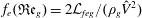
Reference Katoh, Wakimoto, Yamamoto and Ito2015). Several discrepancies between data and functionalities of the form prescribed by Hoffman (Reference Hoffman1975) were also observed by Katoh et al. (Reference Katoh, Wakimoto, Yamamoto and Ito2015). Wu et al. (Reference Wu, Nikolov and Wasan2017) have examined the accuracy of various models. Model validity was also evaluated by Heshmati & Piri (Reference Heshmati and Piri2014) based on data in circular and non-circular tubes with three liquids: glycerol, water and soltrol. Our emphasis here is to predict the rise of hydrocarbons in clean and dry glass capillaries, and we have specifically excluded liquids such as water.
$\tan \unicode[STIX]{x1D703}_{d}(\cos \unicode[STIX]{x1D703}_{d}-\cos \unicode[STIX]{x1D703})$
as a linear function of capillary number for a given roughness predicts capillary rise of diethylene glycol in PMMA capillaries and ethylene glycol in glass capillaries (Katoh et al.
Reference Katoh, Wakimoto, Yamamoto and Ito2015). Several discrepancies between data and functionalities of the form prescribed by Hoffman (Reference Hoffman1975) were also observed by Katoh et al. (Reference Katoh, Wakimoto, Yamamoto and Ito2015). Wu et al. (Reference Wu, Nikolov and Wasan2017) have examined the accuracy of various models. Model validity was also evaluated by Heshmati & Piri (Reference Heshmati and Piri2014) based on data in circular and non-circular tubes with three liquids: glycerol, water and soltrol. Our emphasis here is to predict the rise of hydrocarbons in clean and dry glass capillaries, and we have specifically excluded liquids such as water.
Blake and his coworkers (Blake & Haynes Reference Blake and Haynes1969; Blake Reference Blake2006; Duvivier, Blake & De Coninck Reference Duvivier, Blake and De Coninck2013) analysed work of adhesion and force imbalance due to
 $\unicode[STIX]{x1D703}-\unicode[STIX]{x1D703}_{d}$
. The linearized version of their proposition in terms of a coefficient
$\unicode[STIX]{x1D703}-\unicode[STIX]{x1D703}_{d}$
. The linearized version of their proposition in terms of a coefficient
 $\unicode[STIX]{x1D6FD}$
is
$\unicode[STIX]{x1D6FD}$
is
 $$\begin{eqnarray}\cos \unicode[STIX]{x1D703}_{d}=-\frac{\unicode[STIX]{x1D6FD}\unicode[STIX]{x1D707}_{l}}{\unicode[STIX]{x1D70E}_{lg}}V_{m}(t)+\cos \unicode[STIX]{x1D703}.\end{eqnarray}$$
Evaluation methods of contact angle models was suggested by Popescu, Ralston & Sedev (Reference Popescu, Ralston and Sedev2008). Based on rise data of silicone oils, various alkanes, siloxane and carbon tetrachloride in small borosilicate glass tubes, Wu et al. (Reference Wu, Nikolov and Wasan2017) concluded that many of the models including (3.10) and (3.12) are adequate with an adjustable parameter
 $\unicode[STIX]{x1D712}$
or
$\unicode[STIX]{x1D712}$
or
 $\unicode[STIX]{x1D6FD}$
. All of their tests were conducted for wetting liquids with a precursor film, i.e.
$\unicode[STIX]{x1D6FD}$
. All of their tests were conducted for wetting liquids with a precursor film, i.e.
 $\unicode[STIX]{x1D703}$
was small, but
$\unicode[STIX]{x1D703}$
was small, but
 $\unicode[STIX]{x1D703}_{d}$
may not be. They argued that
$\unicode[STIX]{x1D703}_{d}$
may not be. They argued that
 $\unicode[STIX]{x1D6FD}$
may be estimated for simple molecules. Here, we assume (3.12), with a constant
$\unicode[STIX]{x1D6FD}$
may be estimated for simple molecules. Here, we assume (3.12), with a constant
 $\unicode[STIX]{x1D6FD}$
for a given fluid–solid pair. It has the advantage that analytical solutions may be obtained in the limit of inertia becoming negligible. An evaluation of
$\unicode[STIX]{x1D6FD}$
for a given fluid–solid pair. It has the advantage that analytical solutions may be obtained in the limit of inertia becoming negligible. An evaluation of
 $\unicode[STIX]{x1D6FD}$
from data is possible for an appropriately chosen
$\unicode[STIX]{x1D6FD}$
from data is possible for an appropriately chosen
 $R$
, where dynamic contact angle is important but inertia is not.
$R$
, where dynamic contact angle is important but inertia is not.
The meniscus velocity is approximated by the rate of advance of the meniscus position. Based on data gathered with dioxane, for which
 $\unicode[STIX]{x1D703}$
is
$\unicode[STIX]{x1D703}$
is
 ${>}0\text{}^{\circ }$
, we find that this is better quantified by
${>}0\text{}^{\circ }$
, we find that this is better quantified by
 $h_{e}^{\prime }(t)$
rather than
$h_{e}^{\prime }(t)$
rather than
 $h^{\prime }(t)$
. Then,
$h^{\prime }(t)$
. Then,
 $$\begin{eqnarray}\cos \unicode[STIX]{x1D703}_{d}\approx -\frac{\unicode[STIX]{x1D6FD}\unicode[STIX]{x1D707}_{l}}{\unicode[STIX]{x1D70E}_{lg}}h_{e}^{\prime }(t)+\cos \unicode[STIX]{x1D703}.\end{eqnarray}$$
Also,
 $h_{e}(t)$
is related to
$h_{e}(t)$
is related to
 $h(t)$
through (3.2), and therefore
$h(t)$
through (3.2), and therefore
 $$\begin{eqnarray}h^{\prime }(t)=h_{e}^{\prime }(t)-\frac{1}{3}R{\displaystyle \frac{d\!f(\unicode[STIX]{x1D703}_{d})}{d\!t}}.\end{eqnarray}$$
3.1.8 Outer meniscus
Observations indicate that the surface outside of the capillary oscillates. For example, as shown in figure 4, a magnitude of about 3.5 mm in the inner capillary is concomitant with an outer 0.3 mm in-phase fluctuation for about three cycles. Outer meniscus distance amounts to about
 $3R$
(see figure 4 inset). For an outer meniscus presumed to be a quarter sector of a spherical surface, the volume of revolution within the meniscus is
$3R$
(see figure 4 inset). For an outer meniscus presumed to be a quarter sector of a spherical surface, the volume of revolution within the meniscus is
 $(2/3)(32-9\unicode[STIX]{x03C0})\unicode[STIX]{x03C0}R^{3}$
. Per unit area of the capillary, we approximate this result to
$(2/3)(32-9\unicode[STIX]{x03C0})\unicode[STIX]{x03C0}R^{3}$
. Per unit area of the capillary, we approximate this result to
 $8R/3$
. The velocity of the outer meniscus for oscillations roughly scales as
$8R/3$
. The velocity of the outer meniscus for oscillations roughly scales as
 $(0.3/3.5)\hat{V}$
, giving us a corrected value for the mass for momentum to be added to
$(0.3/3.5)\hat{V}$
, giving us a corrected value for the mass for momentum to be added to
 $m_{R}$
as
$m_{R}$
as
 $(8/35)\unicode[STIX]{x1D70C}$
. We expect the mass to be added to be a multiple of this, comparable to unity. Also,the outer meniscus is included only for
$(8/35)\unicode[STIX]{x1D70C}$
. We expect the mass to be added to be a multiple of this, comparable to unity. Also,the outer meniscus is included only for
 $h_{e}^{\prime }(t)>0$
, because the retraction model’s pressure boundaries are known at the capillary top and bottom.
$h_{e}^{\prime }(t)>0$
, because the retraction model’s pressure boundaries are known at the capillary top and bottom.

Figure 4. Menisci oscillations for diethyl ether (DEE) for
 $L=30~\text{mm}$
and
$L=30~\text{mm}$
and
 $R=1000~\unicode[STIX]{x03BC}\text{m}$
. Inset is a snapshot of the outer meniscus during capillary rise. The white dashed line is the position of the meniscus tip, but is difficult to locate in every frame. All heights are referenced with respect to the red line since only changes are important to identify the scale. Measurement accuracy is about
$R=1000~\unicode[STIX]{x03BC}\text{m}$
. Inset is a snapshot of the outer meniscus during capillary rise. The white dashed line is the position of the meniscus tip, but is difficult to locate in every frame. All heights are referenced with respect to the red line since only changes are important to identify the scale. Measurement accuracy is about
 $34~\unicode[STIX]{x03BC}\text{m}$
.
$34~\unicode[STIX]{x03BC}\text{m}$
.
3.1.9 Hysteresis
The relationship between
 $\unicode[STIX]{x1D703}$
and
$\unicode[STIX]{x1D703}$
and
 $\unicode[STIX]{x1D703}_{d}$
may differ for the advancing and receding interface. Functionally,
$\unicode[STIX]{x1D703}_{d}$
may differ for the advancing and receding interface. Functionally,
 $$\begin{eqnarray}\unicode[STIX]{x1D6FD}=\left\{\begin{array}{@{}ll@{}}\unicode[STIX]{x1D6FD}_{a} & \text{for }h_{m}^{\prime }(t)\geqslant 0,\\ \unicode[STIX]{x1D6FD}_{r} & \text{for }h_{m}^{\prime }(t)<0.\end{array}\right.\end{eqnarray}$$
Here,
 $h_{m}(t)$
is the meniscus position. Alternatively, one may consider that post first contact of the liquid with the solid surface,
$h_{m}(t)$
is the meniscus position. Alternatively, one may consider that post first contact of the liquid with the solid surface,
 $\unicode[STIX]{x1D6FD}$
is assigned a new value, implying film retention on the surface. Consider,
$\unicode[STIX]{x1D6FD}$
is assigned a new value, implying film retention on the surface. Consider,
 $h(t)<h_{M}$
, where
$h(t)<h_{M}$
, where
 $h_{M}$
is the maximum
$h_{M}$
is the maximum
 $h(t)$
, with
$h(t)$
, with
 $h(t_{M})=h_{M}$
. For this model, an algorithm to assign
$h(t_{M})=h_{M}$
. For this model, an algorithm to assign
 $\unicode[STIX]{x1D6FD}$
is
$\unicode[STIX]{x1D6FD}$
is
 $$\begin{eqnarray}\unicode[STIX]{x1D6FD}=\left\{\begin{array}{@{}ll@{}}\unicode[STIX]{x1D6FD}_{a} & \text{for }t\leqslant t_{M},\\ \unicode[STIX]{x1D6FD}_{r} & \text{for }t>t_{M}.\end{array}\right.\end{eqnarray}$$
For computation, we first calculate
 $h_{e}(t)$
assuming
$h_{e}(t)$
assuming
 $\unicode[STIX]{x1D6FD}=\unicode[STIX]{x1D6FD}_{a}$
, and
$\unicode[STIX]{x1D6FD}=\unicode[STIX]{x1D6FD}_{a}$
, and
 $t_{M}$
is located based on either maximum
$t_{M}$
is located based on either maximum
 $h(t)$
or maximum
$h(t)$
or maximum
 $h_{e}(t)$
. In the second pass for integrating rise dynamics equations, equation (3.16) is used, and the differential equations reintegrated with the known initial condition of
$h_{e}(t)$
. In the second pass for integrating rise dynamics equations, equation (3.16) is used, and the differential equations reintegrated with the known initial condition of
 $h_{M}$
at
$h_{M}$
at
 $t_{M}$
with
$t_{M}$
with
 $h^{\prime }(t_{M})=0$
. Implementation of hysteresis was necessary to ascertain its importance. For matching experimental data, no noticeable improvement was observed; therefore, our plots for
$h^{\prime }(t_{M})=0$
. Implementation of hysteresis was necessary to ascertain its importance. For matching experimental data, no noticeable improvement was observed; therefore, our plots for
 $h(t)$
are without hysteresis.
$h(t)$
are without hysteresis.
3.1.10 Oscillations and dimensionless groups
An analysis may be carried out to infer whether oscillations in
 $h(t)$
are likely. While it is necessary to include gas-phase viscous pressure drop, an estimate without it is quite revealing. We recognize two distinct time scales: one with consideration of change of momentum and the other where the characteristic driving force is balanced by a viscosity-induced pressure drop. We denote the latter
$h(t)$
are likely. While it is necessary to include gas-phase viscous pressure drop, an estimate without it is quite revealing. We recognize two distinct time scales: one with consideration of change of momentum and the other where the characteristic driving force is balanced by a viscosity-induced pressure drop. We denote the latter
 $T_{Wo}$
for open-capillary Washburn time. For
$T_{Wo}$
for open-capillary Washburn time. For
 $T_{Wo}$
estimate, we note that the scale for pressure is
$T_{Wo}$
estimate, we note that the scale for pressure is
 $\unicode[STIX]{x1D70C}_{l}gH_{eo}$
. The frictional pressure drop due to liquid viscosity is
$\unicode[STIX]{x1D70C}_{l}gH_{eo}$
. The frictional pressure drop due to liquid viscosity is
 $8\unicode[STIX]{x1D707}_{l}H_{eo}^{2}/(R^{2}T_{Wo})$
. Equating the two, we obtain
$8\unicode[STIX]{x1D707}_{l}H_{eo}^{2}/(R^{2}T_{Wo})$
. Equating the two, we obtain
 $T_{Wo}$
to be
$T_{Wo}$
to be
 $8\unicode[STIX]{x1D707}_{l}H_{eo}/(\unicode[STIX]{x1D70C}_{l}gR^{2})$
. Approximating
$8\unicode[STIX]{x1D707}_{l}H_{eo}/(\unicode[STIX]{x1D70C}_{l}gR^{2})$
. Approximating
 $H_{eo}$
with
$H_{eo}$
with
 $H_{o}$
and replacing
$H_{o}$
and replacing
 $H_{o}$
such that capillary pressure is balanced by liquid-column weight, we get
$H_{o}$
such that capillary pressure is balanced by liquid-column weight, we get
 $$\begin{eqnarray}T_{Wo}=\frac{16\unicode[STIX]{x1D707}_{l}\unicode[STIX]{x1D70E}_{lg}\cos \unicode[STIX]{x1D703}}{\unicode[STIX]{x1D70C}_{l}^{2}g^{2}R^{3}}.\end{eqnarray}$$
This Washburn time estimate is appropriate when
 $\unicode[STIX]{x1D6FD}$
is not materially important.
$\unicode[STIX]{x1D6FD}$
is not materially important.
We contrast this to the time scale
 $T_{IV}$
that is determined by a balance between inertia and viscous drag. Then with
$T_{IV}$
that is determined by a balance between inertia and viscous drag. Then with
 $H_{o}$
in lieu of
$H_{o}$
in lieu of
 $H_{eo}$
,
$H_{eo}$
,
 $\unicode[STIX]{x1D70C}_{l}H_{o}^{2}/T_{IV}^{2}=8\unicode[STIX]{x1D707}_{l}H_{o}^{2}/(R^{2}T_{IV})$
or
$\unicode[STIX]{x1D70C}_{l}H_{o}^{2}/T_{IV}^{2}=8\unicode[STIX]{x1D707}_{l}H_{o}^{2}/(R^{2}T_{IV})$
or
 $$\begin{eqnarray}T_{IV}=\frac{\unicode[STIX]{x1D70C}_{l}R^{2}}{8\unicode[STIX]{x1D707}_{l}}.\end{eqnarray}$$
Our conjecture is that whenever
 $T_{IV}\ll T_{Wo}$
, the Washburn time scale determines the process. When inertia dominates, the time scale
$T_{IV}\ll T_{Wo}$
, the Washburn time scale determines the process. When inertia dominates, the time scale
 $T_{IV}$
dominates the problem, and therefore one would expect oscillations to manifest themselves. The cross-over is given by the ratio
$T_{IV}$
dominates the problem, and therefore one would expect oscillations to manifest themselves. The cross-over is given by the ratio
 $T_{IV}/T_{Wo}={\mathcal{N}}$
, which in terms of known properties is
$T_{IV}/T_{Wo}={\mathcal{N}}$
, which in terms of known properties is
 $$\begin{eqnarray}{\mathcal{N}}=\frac{\unicode[STIX]{x1D70C}_{l}^{3}g^{2}R^{5}}{128\unicode[STIX]{x1D707}_{l}^{2}\unicode[STIX]{x1D70E}_{lg}\cos \unicode[STIX]{x1D703}}.\end{eqnarray}$$
Roughly,
 ${\mathcal{N}}>1$
is expected to promote oscillation. (We are also assuming that when
${\mathcal{N}}>1$
is expected to promote oscillation. (We are also assuming that when
 $T_{IV}<T_{Wo}$
, the height is given by
$T_{IV}<T_{Wo}$
, the height is given by
 $2gT_{IV}^{2}<H_{eo}$
.)
$2gT_{IV}^{2}<H_{eo}$
.)
When
 $\unicode[STIX]{x1D703}\rightarrow 0$
, this dimensionless group may be expressed as
$\unicode[STIX]{x1D703}\rightarrow 0$
, this dimensionless group may be expressed as
 $$\begin{eqnarray}{\mathcal{N}}=\frac{\mathfrak{B}\mathfrak{o}^{2}}{128\mathfrak{O}\mathfrak{h}^{2}},\end{eqnarray}$$
but accounting for contact angle we may also write
 $\mathfrak{B}\mathfrak{o}$
as the Bond number
$\mathfrak{B}\mathfrak{o}$
as the Bond number
 $=\unicode[STIX]{x1D70C}_{l}gR^{2}/(\unicode[STIX]{x1D70E}_{lg}\cos \unicode[STIX]{x1D703})$
, and
$=\unicode[STIX]{x1D70C}_{l}gR^{2}/(\unicode[STIX]{x1D70E}_{lg}\cos \unicode[STIX]{x1D703})$
, and
 $\mathfrak{O}\mathfrak{h}$
as the Ohnesorge number
$\mathfrak{O}\mathfrak{h}$
as the Ohnesorge number
 $=\unicode[STIX]{x1D707}_{l}/(\sqrt{\unicode[STIX]{x1D70C}_{l}R\unicode[STIX]{x1D70E}_{lg}\cos \unicode[STIX]{x1D703}})$
. Equivalently,
$=\unicode[STIX]{x1D707}_{l}/(\sqrt{\unicode[STIX]{x1D70C}_{l}R\unicode[STIX]{x1D70E}_{lg}\cos \unicode[STIX]{x1D703}})$
. Equivalently,
 ${\mathcal{N}}$
is proportional to the product of
${\mathcal{N}}$
is proportional to the product of
 $\mathfrak{B}\mathfrak{o}$
and Galilei numbers, where the latter is
$\mathfrak{B}\mathfrak{o}$
and Galilei numbers, where the latter is
 $\mathfrak{G}\mathfrak{a}=\unicode[STIX]{x1D70C}_{l}^{2}gR^{3}/\unicode[STIX]{x1D707}_{l}^{2}$
. As long as
$\mathfrak{G}\mathfrak{a}=\unicode[STIX]{x1D70C}_{l}^{2}gR^{3}/\unicode[STIX]{x1D707}_{l}^{2}$
. As long as
 $\unicode[STIX]{x1D707}_{g}L\ll \unicode[STIX]{x1D707}_{l}H_{o}$
, and
$\unicode[STIX]{x1D707}_{g}L\ll \unicode[STIX]{x1D707}_{l}H_{o}$
, and
 $\unicode[STIX]{x1D6FD}$
is small, we expect
$\unicode[STIX]{x1D6FD}$
is small, we expect
 ${\mathcal{N}}$
to be a good measure for identifying the importance of inertia. The group presented in (3.20) was also identified by Fries & Dreyer (Reference Fries and Dreyer2008) and Masoodi et al. (Reference Masoodi, Languri and Ostadhossein2013) (barring numerical coefficient), through different arguments. Fries & Dreyer (Reference Fries and Dreyer2008) also represented the group as the product
${\mathcal{N}}$
to be a good measure for identifying the importance of inertia. The group presented in (3.20) was also identified by Fries & Dreyer (Reference Fries and Dreyer2008) and Masoodi et al. (Reference Masoodi, Languri and Ostadhossein2013) (barring numerical coefficient), through different arguments. Fries & Dreyer (Reference Fries and Dreyer2008) also represented the group as the product
 $\mathfrak{B}\mathfrak{o}\mathfrak{G}\mathfrak{a}$
, but their differential equation is quite different and is of the Bosanquet type. The time-scale cross-over was also explicitly proposed by Quéré (Reference Quéré1997).
$\mathfrak{B}\mathfrak{o}\mathfrak{G}\mathfrak{a}$
, but their differential equation is quite different and is of the Bosanquet type. The time-scale cross-over was also explicitly proposed by Quéré (Reference Quéré1997).
The gas column suppresses oscillation. To include its effect, we replace
 $\unicode[STIX]{x1D707}_{l}$
in
$\unicode[STIX]{x1D707}_{l}$
in
 ${\mathcal{N}}$
with
${\mathcal{N}}$
with
 $$\begin{eqnarray}\unicode[STIX]{x1D707}_{e}=\unicode[STIX]{x1D707}_{l}+\unicode[STIX]{x1D707}_{g}\frac{L}{H_{eo}}.\end{eqnarray}$$
The altered dimensionless group for predicting oscillation becomes
 $$\begin{eqnarray}{\mathcal{N}}_{e}=\frac{\unicode[STIX]{x1D70C}_{l}^{3}g^{2}R^{5}}{128\unicode[STIX]{x1D707}_{e}^{2}\unicode[STIX]{x1D70E}_{lg}\cos \unicode[STIX]{x1D703}}.\end{eqnarray}$$
We tabulate both
 ${\mathcal{N}}$
and
${\mathcal{N}}$
and
 ${\mathcal{N}}_{e}$
for the data set. For large
${\mathcal{N}}_{e}$
for the data set. For large
 $\unicode[STIX]{x1D6FD}$
,
$\unicode[STIX]{x1D6FD}$
,
 ${\mathcal{N}}_{e}$
overemphasizes inertia.
${\mathcal{N}}_{e}$
overemphasizes inertia.
3.2 Momentum balance – closed capillary
Here,
 $H_{ec}$
tends to be small compared to
$H_{ec}$
tends to be small compared to
 $H_{eo}$
and is practically observable only for
$H_{eo}$
and is practically observable only for
 $R<200~\unicode[STIX]{x03BC}\text{m}$
. Inertial effects, and therefore losses, are minor, and with
$R<200~\unicode[STIX]{x03BC}\text{m}$
. Inertial effects, and therefore losses, are minor, and with
 $\unicode[STIX]{x1D6FD}$
values for a glass–organics interface, oscillation is suppressed. For the gas phase, inertial effects may be entirely dropped. Closed-capillary rise dynamics, however, introduces some intrinsic mathematical difficulties as a result of the no-flow boundary at the top. Our aim is to derive an expression for
$\unicode[STIX]{x1D6FD}$
values for a glass–organics interface, oscillation is suppressed. For the gas phase, inertial effects may be entirely dropped. Closed-capillary rise dynamics, however, introduces some intrinsic mathematical difficulties as a result of the no-flow boundary at the top. Our aim is to derive an expression for
 $P_{t}$
that includes viscous flow.
$P_{t}$
that includes viscous flow.
3.2.1 Gas pressure,
 $P_{t}$

The increase in gas pressure, though small in relation to
 $P_{0}$
, is comparable to capillary pressure and therefore reduces
$P_{0}$
, is comparable to capillary pressure and therefore reduces
 $H_{e}$
significantly. This necessitates capillaries in the range of tens of microns for
$H_{e}$
significantly. This necessitates capillaries in the range of tens of microns for
 $R$
and hundreds of mm in length for a rise height of a few mm. Inertial terms causing entry and exit losses, and kinetic energy altering entry pressure, are secondary for developing the requisite physics. Gas entry and exit contributions are absent for closed capillaries.
$R$
and hundreds of mm in length for a rise height of a few mm. Inertial terms causing entry and exit losses, and kinetic energy altering entry pressure, are secondary for developing the requisite physics. Gas entry and exit contributions are absent for closed capillaries.
For an ideal gas, the pressure change in the gas phase would scale as
 $P_{0}H_{ec}/L\ll P_{0}$
, and therefore one would be tempted to regard the fluid as incompressible and solve
$P_{0}H_{ec}/L\ll P_{0}$
, and therefore one would be tempted to regard the fluid as incompressible and solve
 $\unicode[STIX]{x2202}^{2}P/\unicode[STIX]{x2202}z^{2}=0$
,
$\unicode[STIX]{x2202}^{2}P/\unicode[STIX]{x2202}z^{2}=0$
,
 $z$
being the vertical coordinate and
$z$
being the vertical coordinate and
 $P$
being the pressure varying with
$P$
being the pressure varying with
 $z$
. Then the dependence on time is assumed to be pseudo-static. The solution having a linear dependence on
$z$
. Then the dependence on time is assumed to be pseudo-static. The solution having a linear dependence on
 $z$
cannot satisfy both of the flux conditions corresponding to a moving boundary at the bottom and closed at the top. Including gas compressibility is necessary.
$z$
cannot satisfy both of the flux conditions corresponding to a moving boundary at the bottom and closed at the top. Including gas compressibility is necessary.
A complete analytical solution to laminar compressible flow within a capillary is unavailable, and is unnecessary given that the dominant dynamics is one-dimensional. Since the pressure change causes negligible change in density on a length scale of
 $R$
, we may ignore compressibility on an
$R$
, we may ignore compressibility on an
 $R$
length scale (but not
$R$
length scale (but not
 $L$
), and express the radially averaged local velocity of gas as
$L$
), and express the radially averaged local velocity of gas as
 $$\begin{eqnarray}\hat{v}_{g}=-\frac{R^{2}}{8\unicode[STIX]{x1D707}_{g}}{\displaystyle \frac{\unicode[STIX]{x2202}P}{\unicode[STIX]{x2202}z}},\end{eqnarray}$$
 $\hat{v}_{g}$
varying with
$\hat{v}_{g}$
varying with
 $z$
and
$z$
and
 $t$
. As explained earlier, gravity terms need not be considered for the purpose of evaluating the pressure profile within the gas phase. Any correction to pressure at the interface, due to gravity, scales with a magnitude of
$t$
. As explained earlier, gravity terms need not be considered for the purpose of evaluating the pressure profile within the gas phase. Any correction to pressure at the interface, due to gravity, scales with a magnitude of
 $\unicode[STIX]{x1D70C}_{g}gH_{ec}^{2}/(2P_{0}L)$
compared to unity and is not relevant. (With
$\unicode[STIX]{x1D70C}_{g}gH_{ec}^{2}/(2P_{0}L)$
compared to unity and is not relevant. (With
 $\unicode[STIX]{x1D70C}_{g}=1~\text{kg}~\text{m}^{-3}$
,
$\unicode[STIX]{x1D70C}_{g}=1~\text{kg}~\text{m}^{-3}$
,
 $H_{ec}=3~\text{mm}$
,
$H_{ec}=3~\text{mm}$
,
 $L=100~\text{mm}$
, this dimensionless quantity has a value of
$L=100~\text{mm}$
, this dimensionless quantity has a value of
 $4.5\times 10^{-10}$
.) From gas-phase continuity,
$4.5\times 10^{-10}$
.) From gas-phase continuity,
 $$\begin{eqnarray}{\displaystyle \frac{\unicode[STIX]{x2202}\unicode[STIX]{x1D70C}_{g}}{\unicode[STIX]{x2202}t}}+{\displaystyle \frac{\unicode[STIX]{x2202}\unicode[STIX]{x1D70C}_{g}\hat{v}_{g}}{\unicode[STIX]{x2202}z}}=0.\end{eqnarray}$$
Since the compressibility factor is nearly unity at atmospheric conditions, the air column is almost an ideal gas. Isothermal compressibility for the column is
 $1/P$
, which to leading order is
$1/P$
, which to leading order is
 $1/P_{0}$
. The pressure scale for the closed-capillary problem is denoted
$1/P_{0}$
. The pressure scale for the closed-capillary problem is denoted
 ${\mathcal{P}}_{c}$
, and this scale applies to represent the deviation from
${\mathcal{P}}_{c}$
, and this scale applies to represent the deviation from
 $P_{0}$
. The change in air pressure due to liquid rise is
$P_{0}$
. The change in air pressure due to liquid rise is
 $P_{0}H_{ec}/(L-H_{ec})$
for an ideal gas, and therefore
$P_{0}H_{ec}/(L-H_{ec})$
for an ideal gas, and therefore
 $$\begin{eqnarray}{\mathcal{P}}_{c}=P_{0}\frac{H_{ec}}{L-H_{ec}}.\end{eqnarray}$$
In contrast to gas-phase isothermal compressibility, defined to be
 $$\begin{eqnarray}c_{g}=\frac{1}{\unicode[STIX]{x1D70C}_{g}}{\displaystyle \frac{\unicode[STIX]{x2202}\unicode[STIX]{x1D70C}_{g}}{\unicode[STIX]{x2202}P}},\end{eqnarray}$$
 $\unicode[STIX]{x1D707}_{g}$
is nearly a constant over the small pressure change of magnitude
$\unicode[STIX]{x1D707}_{g}$
is nearly a constant over the small pressure change of magnitude
 ${\mathcal{P}}_{c}$
, and is therefore fixed. For non-dimensionalization, equations (3.23) and (3.24) require length and time scales. Unlike pressure, two different scales exist for both. The first is the capillary rise time scale as per the Washburn equation, and denoted
${\mathcal{P}}_{c}$
, and is therefore fixed. For non-dimensionalization, equations (3.23) and (3.24) require length and time scales. Unlike pressure, two different scales exist for both. The first is the capillary rise time scale as per the Washburn equation, and denoted
 $T_{Wc}$
. A second time scale is the characteristic time for gas-phase pressure diffusion (
$T_{Wc}$
. A second time scale is the characteristic time for gas-phase pressure diffusion (
 $T_{D}$
) over
$T_{D}$
) over
 $L$
analogous to pressure transients in porous media. The two length scales are
$L$
analogous to pressure transients in porous media. The two length scales are
 $H_{ec}$
and
$H_{ec}$
and
 $L$
. Their ratio
$L$
. Their ratio
 $$\begin{eqnarray}\unicode[STIX]{x1D6FF}=\frac{H_{ec}}{L}\ll 1\end{eqnarray}$$
is a small parameter. A magnitude estimate of
 $\unicode[STIX]{x1D6FF}$
follows from (2.10), where the
$\unicode[STIX]{x1D6FF}$
follows from (2.10), where the
 $P_{0}$
term dominates the denominator. Then,
$P_{0}$
term dominates the denominator. Then,
 $$\begin{eqnarray}\unicode[STIX]{x1D6FF}\approx \frac{2\unicode[STIX]{x1D70E}_{lg}\cos \unicode[STIX]{x1D703}}{RP_{0}}.\end{eqnarray}$$
Where
 $H_{ec}$
is measurably relevant,
$H_{ec}$
is measurably relevant,
 $\unicode[STIX]{x1D6FF}<0.02$
.
$\unicode[STIX]{x1D6FF}<0.02$
.
The Washburn time scale is quantified through the balance between an upward force that is of magnitude
 $\unicode[STIX]{x1D70C}_{l}gH_{ec}$
(note that the magnitude is reflected by the rise height causing a downward body force) and the dominant frictional viscous resistance, resulting in
$\unicode[STIX]{x1D70C}_{l}gH_{ec}$
(note that the magnitude is reflected by the rise height causing a downward body force) and the dominant frictional viscous resistance, resulting in
 $$\begin{eqnarray}T_{Wc}=\frac{8\unicode[STIX]{x1D707}_{l}H_{ec}}{\unicode[STIX]{x1D70C}_{l}gR^{2}}.\end{eqnarray}$$
Similarly, the diffusional time scale for gas pressure is
 $$\begin{eqnarray}T_{D}=\frac{8\unicode[STIX]{x1D707}_{g}L^{2}}{R^{2}P_{0}},\end{eqnarray}$$
where we have recognized the validity of (3.23) for local velocity, with the leading term for compressibility being
 $1/P_{0}$
. We write
$1/P_{0}$
. We write
 $$\begin{eqnarray}\unicode[STIX]{x1D716}\displaystyle :=T_{D}/T_{Wc}=\frac{\unicode[STIX]{x1D707}_{g}\unicode[STIX]{x1D70C}_{l}gL^{2}}{\unicode[STIX]{x1D707}_{l}P_{0}H_{ec}}\ll 1.\end{eqnarray}$$
When
 $H_{ec}$
is replaced from (2.10), we get
$H_{ec}$
is replaced from (2.10), we get
 $$\begin{eqnarray}\unicode[STIX]{x1D716}\approx \frac{\unicode[STIX]{x1D707}_{g}\unicode[STIX]{x1D70C}_{l}gLR}{\unicode[STIX]{x1D707}_{l}2\unicode[STIX]{x1D70E}_{lg}\cos \unicode[STIX]{x1D703}},\end{eqnarray}$$
and it is less than 0.1 for the
 $L$
values used. Replacing
$L$
values used. Replacing
 $\hat{v}_{g}$
from (3.23) in (3.24), and using the expression for isothermal compressibility,
$\hat{v}_{g}$
from (3.23) in (3.24), and using the expression for isothermal compressibility,
 $$\begin{eqnarray}{\displaystyle \frac{\unicode[STIX]{x2202}P}{\unicode[STIX]{x2202}t}}=\frac{R^{2}}{8\unicode[STIX]{x1D707}_{g}}P{\displaystyle \frac{\unicode[STIX]{x2202}2P}{\unicode[STIX]{x2202}z2}}+\frac{R^{2}}{8\unicode[STIX]{x1D707}_{g}}\left({\displaystyle \frac{\unicode[STIX]{x2202}P}{\unicode[STIX]{x2202}z}}\right)^{2}.\end{eqnarray}$$
The dimensionless pressure
 $\unicode[STIX]{x1D713}$
is scaled with respect to
$\unicode[STIX]{x1D713}$
is scaled with respect to
 $\unicode[STIX]{x1D6FF}$
for it to be order unity, i.e.
$\unicode[STIX]{x1D6FF}$
for it to be order unity, i.e.
 $$\begin{eqnarray}\unicode[STIX]{x1D713}=\frac{1}{\unicode[STIX]{x1D6FF}}\frac{P-P_{0}}{P_{0}}\quad \text{or}\quad P=P_{0}(1+\unicode[STIX]{x1D6FF}\unicode[STIX]{x1D713}).\end{eqnarray}$$
Note that
 $\unicode[STIX]{x1D713}$
is to be regarded as a function of the dimensionless time relevant to capillary rise,
$\unicode[STIX]{x1D713}$
is to be regarded as a function of the dimensionless time relevant to capillary rise,
 $$\begin{eqnarray}\unicode[STIX]{x1D70F}_{W}\displaystyle :=t/T_{Wc}=\frac{\unicode[STIX]{x1D70C}_{l}gR^{2}t}{8\unicode[STIX]{x1D707}_{l}H_{ec}},\end{eqnarray}$$
the dimensionless time relevant to diffusion,
 $$\begin{eqnarray}\unicode[STIX]{x1D70F}_{D}\displaystyle :=t/T_{D}=\frac{P_{0}R^{2}t}{8\unicode[STIX]{x1D707}_{g}L^{2}},\end{eqnarray}$$
and
 $\unicode[STIX]{x1D701}$
, the dimensionless distance from the closed end, i.e.
$\unicode[STIX]{x1D701}$
, the dimensionless distance from the closed end, i.e.
 $$\begin{eqnarray}\unicode[STIX]{x1D701}\displaystyle :=\frac{L-z}{L}\,.\end{eqnarray}$$
The dimensionless form of (3.33) is
 $$\begin{eqnarray}\unicode[STIX]{x1D716}{\displaystyle \frac{\unicode[STIX]{x2202}\unicode[STIX]{x1D713}}{\unicode[STIX]{x2202}\unicode[STIX]{x1D70F}_{W}}}=(1+\unicode[STIX]{x1D6FF}\unicode[STIX]{x1D713}){\displaystyle \frac{\unicode[STIX]{x2202}2\unicode[STIX]{x1D713}}{\unicode[STIX]{x2202}\unicode[STIX]{x1D701}2}}+\unicode[STIX]{x1D6FF}\left({\displaystyle \frac{\unicode[STIX]{x2202}\unicode[STIX]{x1D713}}{\unicode[STIX]{x2202}\unicode[STIX]{x1D701}}}\right)^{2},\end{eqnarray}$$
where we seek only the functional dependence of
 $\unicode[STIX]{x1D713}$
on
$\unicode[STIX]{x1D713}$
on
 $\unicode[STIX]{x1D70F}_{W}$
and
$\unicode[STIX]{x1D70F}_{W}$
and
 $\unicode[STIX]{x1D701}$
, since
$\unicode[STIX]{x1D701}$
, since
 $T_{Wc}\gg T_{D}$
. For solving (3.38), we satisfy zero flow at the top (
$T_{Wc}\gg T_{D}$
. For solving (3.38), we satisfy zero flow at the top (
 $\unicode[STIX]{x1D701}=0$
) and that the velocity of liquid must equal the velocity of gas at the meniscus. The first boundary condition is
$\unicode[STIX]{x1D701}=0$
) and that the velocity of liquid must equal the velocity of gas at the meniscus. The first boundary condition is
 $$\begin{eqnarray}{\displaystyle \frac{\unicode[STIX]{x2202}\unicode[STIX]{x1D713}}{\unicode[STIX]{x2202}\unicode[STIX]{x1D701}}}=0,\quad \text{at }\unicode[STIX]{x1D701}=0.\end{eqnarray}$$
For the second boundary condition, we observe that the dimensionless rise height,
 $h_{e}(t)/H_{ec}$
, must be a function only of
$h_{e}(t)/H_{ec}$
, must be a function only of
 $\unicode[STIX]{x1D70F}_{W}$
. We define
$\unicode[STIX]{x1D70F}_{W}$
. We define
 $$\begin{eqnarray}\unicode[STIX]{x1D702}(\unicode[STIX]{x1D70F}_{W})\displaystyle :=\frac{h_{e}(t)}{H_{ec}}.\end{eqnarray}$$
Then, at the bottom moving boundary of the air column,
 $$\begin{eqnarray}{\displaystyle \frac{ d\!h_{e}(t)}{d\!t}}=-\frac{R^{2}}{8\unicode[STIX]{x1D707}_{g}}{\displaystyle \frac{\unicode[STIX]{x2202}p}{\unicode[STIX]{x2202}z}},\quad \text{at }z=h_{e}(t).\end{eqnarray}$$
In dimensionless form, this translates to
 $$\begin{eqnarray}{\displaystyle \frac{\unicode[STIX]{x2202}\unicode[STIX]{x1D713}}{\unicode[STIX]{x2202}\unicode[STIX]{x1D701}}}=\unicode[STIX]{x1D716}{\displaystyle \frac{d\!\unicode[STIX]{x1D702}(\unicode[STIX]{x1D70F}_{W})}{d\!\unicode[STIX]{x1D70F}_{W}}},\quad \text{at }\unicode[STIX]{x1D701}=1-\unicode[STIX]{x1D6FF}\unicode[STIX]{x1D702}(\unicode[STIX]{x1D70F}_{W}).\end{eqnarray}$$
Also the initial condition for pressure in a column of length
 $L$
is
$L$
is
 $$\begin{eqnarray}P=P_{0},\quad \text{at }\unicode[STIX]{x1D70F}_{W}=0.\end{eqnarray}$$
Furthermore, for mass conservation
 $$\begin{eqnarray}P_{0}L=\int _{0}^{L-h_{e}(t)}P\,d\!y=P_{0}L(1-\unicode[STIX]{x1D6FF}\unicode[STIX]{x1D702}(\unicode[STIX]{x1D70F}_{W}))+P_{0}L\unicode[STIX]{x1D6FF}\int _{0}^{1-\unicode[STIX]{x1D6FF}\unicode[STIX]{x1D702}(\unicode[STIX]{x1D70F}_{W})}\unicode[STIX]{x1D713} d\!\unicode[STIX]{x1D701},\end{eqnarray}$$
since
 $P$
is proportional to density. In dimensionless form, this reduces to
$P$
is proportional to density. In dimensionless form, this reduces to
 $$\begin{eqnarray}\int _{0}^{1-\unicode[STIX]{x1D6FF}\unicode[STIX]{x1D702}(\unicode[STIX]{x1D70F}_{W})}\unicode[STIX]{x1D713} d\!\unicode[STIX]{x1D701}=\unicode[STIX]{x1D702}(\unicode[STIX]{x1D70F}_{W}).\end{eqnarray}$$
We seek an ansatz solution of the form
 $$\begin{eqnarray}\unicode[STIX]{x1D713}=\unicode[STIX]{x1D713}_{0}+\unicode[STIX]{x1D716}(\unicode[STIX]{x1D713}_{1}+\unicode[STIX]{x1D6FF}\unicode[STIX]{x1D713}_{2})+\cdots \,,\end{eqnarray}$$
for which the differential equation (3.38) becomes
 $$\begin{eqnarray}\displaystyle \unicode[STIX]{x1D716}{\displaystyle \frac{\unicode[STIX]{x2202}\unicode[STIX]{x1D713}_{0}}{\unicode[STIX]{x2202}\unicode[STIX]{x1D70F}_{W}}}+\unicode[STIX]{x1D716}^{2}{\displaystyle \frac{\unicode[STIX]{x2202}\unicode[STIX]{x1D713}_{1}}{\unicode[STIX]{x2202}\unicode[STIX]{x1D70F}_{W}}} & = & \displaystyle {\displaystyle \frac{\unicode[STIX]{x2202}2\unicode[STIX]{x1D713}_{0}}{\unicode[STIX]{x2202}\unicode[STIX]{x1D701}2}}+\unicode[STIX]{x1D716}{\displaystyle \frac{\unicode[STIX]{x2202}2\unicode[STIX]{x1D713}_{1}}{\unicode[STIX]{x2202}\unicode[STIX]{x1D701}2}}+\unicode[STIX]{x1D6FF}\unicode[STIX]{x1D713}_{0}{\displaystyle \frac{\unicode[STIX]{x2202}2\unicode[STIX]{x1D713}_{0}}{\unicode[STIX]{x2202}\unicode[STIX]{x1D701}2}}+\unicode[STIX]{x1D6FF}\left({\displaystyle \frac{\unicode[STIX]{x2202}\unicode[STIX]{x1D713}_{0}}{\unicode[STIX]{x2202}\unicode[STIX]{x1D701}}}\right)^{2}\nonumber\\ \displaystyle & & \displaystyle +\,\unicode[STIX]{x1D716}\unicode[STIX]{x1D6FF}\left({\displaystyle \frac{\unicode[STIX]{x2202}2\unicode[STIX]{x1D713}_{2}}{\unicode[STIX]{x2202}\unicode[STIX]{x1D701}2}}+\unicode[STIX]{x1D713}_{1}{\displaystyle \frac{\unicode[STIX]{x2202}2\unicode[STIX]{x1D713}_{0}}{\unicode[STIX]{x2202}\unicode[STIX]{x1D701}2}}+\unicode[STIX]{x1D713}_{0}{\displaystyle \frac{\unicode[STIX]{x2202}2\unicode[STIX]{x1D713}_{1}}{\unicode[STIX]{x2202}\unicode[STIX]{x1D701}2}}+2{\displaystyle \frac{\unicode[STIX]{x2202}\unicode[STIX]{x1D713}_{0}}{\unicode[STIX]{x2202}\unicode[STIX]{x1D701}}}{\displaystyle \frac{\unicode[STIX]{x2202}\unicode[STIX]{x1D713}_{1}}{\unicode[STIX]{x2202}\unicode[STIX]{x1D701}}}\right)+\cdots \,.\nonumber\\ \displaystyle & & \displaystyle\end{eqnarray}$$
The leading-order differential equation is
 $$\begin{eqnarray}{\displaystyle \frac{\unicode[STIX]{x2202}2\unicode[STIX]{x1D713}_{0}}{\unicode[STIX]{x2202}\unicode[STIX]{x1D701}2}}=0,\end{eqnarray}$$
the solution to which is
 $$\begin{eqnarray}\unicode[STIX]{x1D713}_{0}(\unicode[STIX]{x1D701},\unicode[STIX]{x1D70F}_{W})=A(\unicode[STIX]{x1D70F}_{W})\unicode[STIX]{x1D701}+F(\unicode[STIX]{x1D70F}_{W}),\end{eqnarray}$$
where
 $A$
and
$A$
and
 $F$
are to be determined. The boundary condition at
$F$
are to be determined. The boundary condition at
 $\unicode[STIX]{x1D701}=0$
implies
$\unicode[STIX]{x1D701}=0$
implies
 $A(\unicode[STIX]{x1D70F}_{W})=0$
, or
$A(\unicode[STIX]{x1D70F}_{W})=0$
, or
 $$\begin{eqnarray}\unicode[STIX]{x1D713}_{0}(\unicode[STIX]{x1D701},\unicode[STIX]{x1D70F}_{W})=F(\unicode[STIX]{x1D70F}_{W}).\end{eqnarray}$$
Physically, for leading order, or
 $\unicode[STIX]{x1D716}=0$
, the only acceptable solution is that the pressure is a constant in the air column for a given
$\unicode[STIX]{x1D716}=0$
, the only acceptable solution is that the pressure is a constant in the air column for a given
 $\unicode[STIX]{x1D70F}_{W}$
. From (3.45) we get
$\unicode[STIX]{x1D70F}_{W}$
. From (3.45) we get
 $$\begin{eqnarray}F(\unicode[STIX]{x1D70F}_{W})=\frac{\unicode[STIX]{x1D702}(\unicode[STIX]{x1D70F}_{W})}{1-\unicode[STIX]{x1D6FF}\unicode[STIX]{x1D702}(\unicode[STIX]{x1D70F}_{W})}.\end{eqnarray}$$
At
 $\unicode[STIX]{x1D701}=1-\unicode[STIX]{x1D6FF}\unicode[STIX]{x1D702}(\unicode[STIX]{x1D70F}_{W})$
, the required boundary condition (3.42) becomes
$\unicode[STIX]{x1D701}=1-\unicode[STIX]{x1D6FF}\unicode[STIX]{x1D702}(\unicode[STIX]{x1D70F}_{W})$
, the required boundary condition (3.42) becomes
 $$\begin{eqnarray}{\displaystyle \frac{\unicode[STIX]{x2202}\unicode[STIX]{x1D713}_{0}}{\unicode[STIX]{x2202}\unicode[STIX]{x1D701}}}=0.\end{eqnarray}$$
This is automatically satisfied by (3.50).
Recognizing (3.50), or
 $\unicode[STIX]{x2202}\unicode[STIX]{x1D713}_{0}/\unicode[STIX]{x2202}\unicode[STIX]{x1D701}=0$
, and matching terms of order
$\unicode[STIX]{x2202}\unicode[STIX]{x1D713}_{0}/\unicode[STIX]{x2202}\unicode[STIX]{x1D701}=0$
, and matching terms of order
 $\unicode[STIX]{x1D716}$
,
$\unicode[STIX]{x1D716}$
,
 $$\begin{eqnarray}{\displaystyle \frac{\unicode[STIX]{x2202}2\unicode[STIX]{x1D713}_{1}}{\unicode[STIX]{x2202}\unicode[STIX]{x1D701}2}}={\displaystyle \frac{\unicode[STIX]{x2202}\unicode[STIX]{x1D713}_{0}}{\unicode[STIX]{x2202}\unicode[STIX]{x1D70F}_{W}}}=\frac{\unicode[STIX]{x1D702}^{\prime }(\unicode[STIX]{x1D70F}_{W})}{\{1-\unicode[STIX]{x1D6FF}\unicode[STIX]{x1D702}(\unicode[STIX]{x1D70F}_{W})\}^{2}},\end{eqnarray}$$
which when integrated results in
 $$\begin{eqnarray}{\displaystyle \frac{\unicode[STIX]{x2202}\unicode[STIX]{x1D713}_{1}}{\unicode[STIX]{x2202}\unicode[STIX]{x1D701}}}=\frac{\unicode[STIX]{x1D702}^{\prime }(\unicode[STIX]{x1D70F}_{W})}{\{1-\unicode[STIX]{x1D6FF}\unicode[STIX]{x1D702}(\unicode[STIX]{x1D70F}_{W})\}^{2}}\unicode[STIX]{x1D701}+G(\unicode[STIX]{x1D70F}_{W}).\end{eqnarray}$$
From the boundary condition at
 $\unicode[STIX]{x1D701}=0$
,
$\unicode[STIX]{x1D701}=0$
,
 $\unicode[STIX]{x2202}\unicode[STIX]{x1D713}/\unicode[STIX]{x2202}\unicode[STIX]{x1D701}=0$
or
$\unicode[STIX]{x2202}\unicode[STIX]{x1D713}/\unicode[STIX]{x2202}\unicode[STIX]{x1D701}=0$
or
 $G(\unicode[STIX]{x1D70F}_{W})=0$
. Then
$G(\unicode[STIX]{x1D70F}_{W})=0$
. Then
 $$\begin{eqnarray}\unicode[STIX]{x1D713}_{1}(\unicode[STIX]{x1D701},\unicode[STIX]{x1D70F}_{W})=\frac{\unicode[STIX]{x1D702}^{\prime }(\unicode[STIX]{x1D70F}_{W})}{\{1-\unicode[STIX]{x1D6FF}\unicode[STIX]{x1D702}(\unicode[STIX]{x1D70F}_{W})\}^{2}}\frac{\unicode[STIX]{x1D701}^{2}}{2}+M(\unicode[STIX]{x1D70F}_{W}),\end{eqnarray}$$
and
 $M(\unicode[STIX]{x1D70F}_{W})$
may be determined from mass conservation. Following (3.45), we find that
$M(\unicode[STIX]{x1D70F}_{W})$
may be determined from mass conservation. Following (3.45), we find that
 $$\begin{eqnarray}M(\unicode[STIX]{x1D70F}_{W})=-\frac{\unicode[STIX]{x1D702}^{\prime }(\unicode[STIX]{x1D70F}_{W})}{6}.\end{eqnarray}$$
The solution is
 $$\begin{eqnarray}\unicode[STIX]{x1D713}(\unicode[STIX]{x1D70F}_{W},\unicode[STIX]{x1D701})=\frac{\unicode[STIX]{x1D702}(\unicode[STIX]{x1D70F}_{W})}{1-\unicode[STIX]{x1D6FF}\unicode[STIX]{x1D702}(\unicode[STIX]{x1D70F}_{W})}+\unicode[STIX]{x1D716}\left[\frac{\unicode[STIX]{x1D702}^{\prime }(\unicode[STIX]{x1D70F}_{W})}{\{1-\unicode[STIX]{x1D6FF}\unicode[STIX]{x1D702}(\unicode[STIX]{x1D70F}_{W})\}^{2}}\frac{\unicode[STIX]{x1D701}^{2}}{2}-\frac{\unicode[STIX]{x1D702}^{\prime }(\unicode[STIX]{x1D70F}_{W})}{6}\right]+\cdots \,.\end{eqnarray}$$
Expanding the boundary condition (3.42), we have
 $$\begin{eqnarray}{\displaystyle \frac{\unicode[STIX]{x2202}\unicode[STIX]{x1D713}_{0}}{\unicode[STIX]{x2202}\unicode[STIX]{x1D701}}}+\unicode[STIX]{x1D716}{\displaystyle \frac{\unicode[STIX]{x2202}\unicode[STIX]{x1D713}_{1}}{\unicode[STIX]{x2202}\unicode[STIX]{x1D701}}}+\cdots =\unicode[STIX]{x1D716}{\displaystyle \frac{d\!\unicode[STIX]{x1D702}(\unicode[STIX]{x1D70F}_{W})}{d\!\unicode[STIX]{x1D70F}_{W}}},\quad \text{at }\unicode[STIX]{x1D701}=1-\unicode[STIX]{x1D6FF}\unicode[STIX]{x1D702}(\unicode[STIX]{x1D70F}_{W}).\end{eqnarray}$$
This is satisfied by the result in (3.57), since they match to the order of
 $\unicode[STIX]{x1D716}$
. Now, matching
$\unicode[STIX]{x1D716}$
. Now, matching
 $\unicode[STIX]{x1D6FF}\unicode[STIX]{x1D716}$
terms, we get
$\unicode[STIX]{x1D6FF}\unicode[STIX]{x1D716}$
terms, we get
 $$\begin{eqnarray}{\displaystyle \frac{\unicode[STIX]{x2202}2\unicode[STIX]{x1D713}_{2}}{\unicode[STIX]{x2202}\unicode[STIX]{x1D701}2}}+\unicode[STIX]{x1D713}_{1}{\displaystyle \frac{\unicode[STIX]{x2202}2\unicode[STIX]{x1D713}_{0}}{\unicode[STIX]{x2202}\unicode[STIX]{x1D701}2}}+\unicode[STIX]{x1D713}_{0}{\displaystyle \frac{\unicode[STIX]{x2202}2\unicode[STIX]{x1D713}_{1}}{\unicode[STIX]{x2202}\unicode[STIX]{x1D701}2}}+2{\displaystyle \frac{\unicode[STIX]{x2202}\unicode[STIX]{x1D713}_{0}}{\unicode[STIX]{x2202}\unicode[STIX]{x1D701}}}{\displaystyle \frac{\unicode[STIX]{x2202}\unicode[STIX]{x1D713}_{1}}{\unicode[STIX]{x2202}\unicode[STIX]{x1D701}}}=0.\end{eqnarray}$$
But in the above equation, we see that the second and fourth terms are zero, for
 $\unicode[STIX]{x2202}\unicode[STIX]{x1D713}_{0}/\unicode[STIX]{x2202}\unicode[STIX]{x1D701}=0$
. We may also replace the
$\unicode[STIX]{x2202}\unicode[STIX]{x1D713}_{0}/\unicode[STIX]{x2202}\unicode[STIX]{x1D701}=0$
. We may also replace the
 $\unicode[STIX]{x2202}^{2}\unicode[STIX]{x1D713}_{1}/\unicode[STIX]{x2202}\unicode[STIX]{x1D701}^{2}$
term with the result from (3.53). The differential equation simplifies to
$\unicode[STIX]{x2202}^{2}\unicode[STIX]{x1D713}_{1}/\unicode[STIX]{x2202}\unicode[STIX]{x1D701}^{2}$
term with the result from (3.53). The differential equation simplifies to
 $$\begin{eqnarray}{\displaystyle \frac{\unicode[STIX]{x2202}2\unicode[STIX]{x1D713}_{2}}{\unicode[STIX]{x2202}\unicode[STIX]{x1D701}2}}=-\frac{\unicode[STIX]{x1D702}(\unicode[STIX]{x1D70F}_{W})\unicode[STIX]{x1D702}^{\prime }(\unicode[STIX]{x1D70F}_{W})}{\{1-\unicode[STIX]{x1D6FF}\unicode[STIX]{x1D702}(\unicode[STIX]{x1D70F}_{W})\}^{3}}.\end{eqnarray}$$
We may again use the
 $\unicode[STIX]{x1D701}=0$
boundary condition to infer that
$\unicode[STIX]{x1D701}=0$
boundary condition to infer that
 $$\begin{eqnarray}{\displaystyle \frac{\unicode[STIX]{x2202}\unicode[STIX]{x1D713}_{2}}{\unicode[STIX]{x2202}\unicode[STIX]{x1D701}}}=-\frac{\unicode[STIX]{x1D702}(\unicode[STIX]{x1D70F}_{W})\unicode[STIX]{x1D702}^{\prime }(\unicode[STIX]{x1D70F}_{W})}{\{1-\unicode[STIX]{x1D6FF}\unicode[STIX]{x1D702}(\unicode[STIX]{x1D70F}_{W})\}^{3}}\unicode[STIX]{x1D701}\end{eqnarray}$$
or
 $$\begin{eqnarray}\unicode[STIX]{x1D713}_{2}=-\frac{\unicode[STIX]{x1D702}(\unicode[STIX]{x1D70F}_{W})\unicode[STIX]{x1D702}^{\prime }(\unicode[STIX]{x1D70F}_{W})}{\{1-\unicode[STIX]{x1D6FF}\unicode[STIX]{x1D702}(\unicode[STIX]{x1D70F}_{W})\}^{3}}\frac{\unicode[STIX]{x1D701}^{2}}{2}+N(\unicode[STIX]{x1D70F}_{W}),\end{eqnarray}$$
where
 $N(\unicode[STIX]{x1D70F}_{W})$
needs to be determined. As before, from the mass conservation criterion,
$N(\unicode[STIX]{x1D70F}_{W})$
needs to be determined. As before, from the mass conservation criterion,
 $$\begin{eqnarray}N(\unicode[STIX]{x1D70F}_{W})=\frac{\unicode[STIX]{x1D702}(\unicode[STIX]{x1D70F}_{W})\unicode[STIX]{x1D702}^{\prime }(\unicode[STIX]{x1D70F}_{W})}{6\{1-\unicode[STIX]{x1D6FF}\unicode[STIX]{x1D702}(\unicode[STIX]{x1D70F}_{W})\}}.\end{eqnarray}$$
The solution then is
 $$\begin{eqnarray}\displaystyle \unicode[STIX]{x1D713}(\unicode[STIX]{x1D70F}_{W},\unicode[STIX]{x1D701}) & = & \displaystyle \frac{\unicode[STIX]{x1D702}(\unicode[STIX]{x1D70F}_{W})}{1-\unicode[STIX]{x1D6FF}\unicode[STIX]{x1D702}(\unicode[STIX]{x1D70F}_{W})}+\unicode[STIX]{x1D716}\left[\frac{\unicode[STIX]{x1D702}^{\prime }(\unicode[STIX]{x1D70F}_{W})}{\{1-\unicode[STIX]{x1D6FF}\unicode[STIX]{x1D702}(\unicode[STIX]{x1D70F}_{W})\}^{2}}\frac{\unicode[STIX]{x1D701}^{2}}{2}-\frac{\unicode[STIX]{x1D702}^{\prime }(\unicode[STIX]{x1D70F}_{W})}{6}\right]\nonumber\\ \displaystyle & & \displaystyle \quad +\,\unicode[STIX]{x1D716}\unicode[STIX]{x1D6FF}\left[\frac{\unicode[STIX]{x1D702}(\unicode[STIX]{x1D70F}_{W})\unicode[STIX]{x1D702}^{\prime }(\unicode[STIX]{x1D70F}_{W})}{6\{1-\unicode[STIX]{x1D6FF}\unicode[STIX]{x1D702}(\unicode[STIX]{x1D70F}_{W})\}}-\frac{\unicode[STIX]{x1D702}(\unicode[STIX]{x1D70F}_{W})\unicode[STIX]{x1D702}^{\prime }(\unicode[STIX]{x1D70F}_{W})}{\{1-\unicode[STIX]{x1D6FF}\unicode[STIX]{x1D702}(\unicode[STIX]{x1D70F}_{W})\}^{3}}\frac{\unicode[STIX]{x1D701}^{2}}{2}\right]+\cdots \,.\end{eqnarray}$$
Now,
 $$\begin{eqnarray}{\displaystyle \frac{\unicode[STIX]{x2202}\unicode[STIX]{x1D713}}{\unicode[STIX]{x2202}\unicode[STIX]{x1D701}}}(\unicode[STIX]{x1D70F}_{W},1-\unicode[STIX]{x1D6FF}\unicode[STIX]{x1D702}(\unicode[STIX]{x1D70F}_{W}))=\unicode[STIX]{x1D716}\frac{\unicode[STIX]{x1D702}^{\prime }(\unicode[STIX]{x1D70F}_{W})}{1-\unicode[STIX]{x1D6FF}\unicode[STIX]{x1D702}(\unicode[STIX]{x1D70F}_{W})}-\unicode[STIX]{x1D716}\unicode[STIX]{x1D6FF}\left[\frac{\unicode[STIX]{x1D702}(\unicode[STIX]{x1D70F}_{W})\unicode[STIX]{x1D702}^{\prime }(\unicode[STIX]{x1D70F}_{W})}{\{1-\unicode[STIX]{x1D6FF}\unicode[STIX]{x1D702}(\unicode[STIX]{x1D70F}_{W})\}^{2}}\right]=\unicode[STIX]{x1D716}\unicode[STIX]{x1D702}^{\prime }(\unicode[STIX]{x1D70F}_{W})+o(\unicode[STIX]{x1D716}\unicode[STIX]{x1D6FF}).\end{eqnarray}$$
The boundary condition is correct to the order of the expansion sought. At this order, the expansion far exceeds the resolution or the reproducibility of the experiment. For rise dynamics formulation, the pressure at the interface in dimensionless form is
 $$\begin{eqnarray}\unicode[STIX]{x1D713}(\unicode[STIX]{x1D70F}_{W},1-\unicode[STIX]{x1D6FF}\unicode[STIX]{x1D702}(\unicode[STIX]{x1D70F}_{W}))=\frac{\unicode[STIX]{x1D702}(\unicode[STIX]{x1D70F}_{W})}{1-\unicode[STIX]{x1D6FF}\unicode[STIX]{x1D702}(\unicode[STIX]{x1D70F}_{W})}+\unicode[STIX]{x1D716}\frac{\unicode[STIX]{x1D702}^{\prime }(\unicode[STIX]{x1D70F}_{W})}{3}-\unicode[STIX]{x1D716}\unicode[STIX]{x1D6FF}\frac{\unicode[STIX]{x1D702}(\unicode[STIX]{x1D70F}_{W})\unicode[STIX]{x1D702}^{\prime }(\unicode[STIX]{x1D70F}_{W})}{3\{1-\unicode[STIX]{x1D6FF}\unicode[STIX]{x1D702}(\unicode[STIX]{x1D70F}_{W})\}}+o(\unicode[STIX]{x1D716}\unicode[STIX]{x1D6FF}).\end{eqnarray}$$
Air pressure just above the meniscus is then
 $$\begin{eqnarray}P(t,h_{e}(t))=P_{0}\left[\frac{L}{L-h_{e}(t)}+\frac{8\unicode[STIX]{x1D707}_{g}\{L-h_{e}(t)\}}{3R^{2}P_{0}}{\displaystyle \frac{ d\!h_{e}(t)}{d\!t}}-\frac{h_{e}^{2}(t)}{L-h_{e}(t)}\frac{8\unicode[STIX]{x1D707}_{g}}{3R^{2}P_{0}}{\displaystyle \frac{ d\!h_{e}(t)}{d\!t}}+\cdots \,\right].\end{eqnarray}$$
The third term may be neglected since it is numerically inconsequential. The equilibrium pressure
 $P_{tc}$
is the first term. Since
$P_{tc}$
is the first term. Since
 $P(t,h_{e}(t))$
is
$P(t,h_{e}(t))$
is
 $P_{t}$
, we have
$P_{t}$
, we have
 $$\begin{eqnarray}P_{t}\sim P_{tc}+\frac{8\unicode[STIX]{x1D707}_{g}\{L-h_{e}(t)\}}{3R^{2}}{\displaystyle \frac{ d\!h_{e}(t)}{d\!t}}.\end{eqnarray}$$
Note that the closed-capillary gas flow viscous-drag term has
 $8/3$
numerical prefactor.
$8/3$
numerical prefactor.
3.2.2 Consolidated formulation
While the liquid loss terms survive from the open-capillary analysis, the gas terms are no longer applicable. The derivation for
 $P_{t}$
ignores inertia in the gas phase. Additionally, the gravity term in the gas phase has already been shown to be negligible. With
$P_{t}$
ignores inertia in the gas phase. Additionally, the gravity term in the gas phase has already been shown to be negligible. With
 $P_{t}$
explicitly known, the dynamics in a closed capillary is then
$P_{t}$
explicitly known, the dynamics in a closed capillary is then
 $$\begin{eqnarray}\displaystyle & & \displaystyle \frac{1}{2}\unicode[STIX]{x1D70C}_{l}h_{e}^{\prime 2}(t)+\unicode[STIX]{x1D70C}_{l}h_{e}(t)h_{e}^{\prime \prime }(t)+(Rm_{Rl}(\mathfrak{R}\mathfrak{e}_{l})h_{e}^{\prime \prime }(t)+Rm_{Rl}^{\prime }(\mathfrak{R}\mathfrak{e}_{l})h_{e}^{\prime }(t))\left\{\frac{S(h_{e}^{\prime }(t))+1}{2}\right\}\nonumber\\ \displaystyle & & \displaystyle \quad -\,2\frac{\unicode[STIX]{x1D70E}_{lg}}{R}\cos \unicode[STIX]{x1D703}_{d}+\frac{8}{R^{2}}\unicode[STIX]{x1D707}_{l}h_{e}(t)h_{e}^{\prime }(t)+\frac{P_{0}h_{e}(t)}{L-h_{e}(t)}+\frac{8\unicode[STIX]{x1D707}_{g}}{3R^{2}}(L-h_{e}(t))h_{e}^{\prime }(t)\nonumber\\ \displaystyle & & \displaystyle \quad +\,\unicode[STIX]{x1D70C}_{l}gh_{e}(t)+{\mathcal{L}}_{frl}(\mathfrak{R}\mathfrak{e}_{l})\left\{\frac{S(h_{e}^{\prime }(t))+1}{2}\right\}-{\mathcal{L}}_{fel}(\mathfrak{R}\mathfrak{e}_{l})\left\{\frac{-S(h_{e}^{\prime }(t))+1}{2}\right\}\nonumber\\ \displaystyle & & \displaystyle \quad -\,\frac{5}{6}\unicode[STIX]{x1D70C}_{l}h_{e}^{\prime 2}\left\{\frac{-S(h_{e}^{\prime }(t))+1}{2}\right\}=0.\end{eqnarray}$$
3.2.3 Closed-capillary dimensionless groups
For the closed-capillary problem, the inertial–viscous time scale is unaltered and is
 $$\begin{eqnarray}T_{IV}=\frac{\unicode[STIX]{x1D70C}_{l}R^{2}}{8\unicode[STIX]{x1D707}_{l}}.\end{eqnarray}$$
Replacing
 $H_{ec}$
in (3.29) with
$H_{ec}$
in (3.29) with
 $2\unicode[STIX]{x1D70E}_{lg}L\cos \unicode[STIX]{x1D703}/(RP_{0})$
(see (2.10)), we get
$2\unicode[STIX]{x1D70E}_{lg}L\cos \unicode[STIX]{x1D703}/(RP_{0})$
(see (2.10)), we get
 $$\begin{eqnarray}T_{Wc}=\frac{16\unicode[STIX]{x1D70E}_{lg}\unicode[STIX]{x1D707}_{l}L\cos \unicode[STIX]{x1D703}}{\unicode[STIX]{x1D70C}_{l}gP_{0}R^{3}}.\end{eqnarray}$$
Along the lines of the open-capillary problem, the ratio
 $T_{IV}/T_{W}$
is defined to be
$T_{IV}/T_{W}$
is defined to be
 $$\begin{eqnarray}{\mathcal{M}}=\frac{\unicode[STIX]{x1D70C}_{l}^{2}R^{5}gP_{0}}{128\unicode[STIX]{x1D707}_{l}^{2}\unicode[STIX]{x1D70E}_{lg}L\cos \unicode[STIX]{x1D703}}.\end{eqnarray}$$
When gas-phase pressure drop affects rise rate, for closed capillaries we let
 $$\begin{eqnarray}\unicode[STIX]{x1D707}_{e}=\unicode[STIX]{x1D707}_{l}+\unicode[STIX]{x1D707}_{g}\frac{L}{3H_{ec}}\end{eqnarray}$$
to reflect the
 $8/3$
coefficient in expression (3.68) so that
$8/3$
coefficient in expression (3.68) so that
 $$\begin{eqnarray}{\mathcal{M}}_{e}=\frac{\unicode[STIX]{x1D70C}_{l}^{2}R^{5}gP_{0}}{128\unicode[STIX]{x1D707}_{e}^{2}\unicode[STIX]{x1D70E}_{lg}L\cos \unicode[STIX]{x1D703}}.\end{eqnarray}$$
Analogous to the open-capillary problem, one might have expected
 ${\mathcal{M}}_{e}$
to be a good indicator of oscillations, if one ignores the shift from
${\mathcal{M}}_{e}$
to be a good indicator of oscillations, if one ignores the shift from
 $\unicode[STIX]{x1D703}$
to
$\unicode[STIX]{x1D703}$
to
 $\unicode[STIX]{x1D703}_{d}$
. But unlike the open-capillary problem where
$\unicode[STIX]{x1D703}_{d}$
. But unlike the open-capillary problem where
 $H_{eo}$
is sufficiently large to be greater than
$H_{eo}$
is sufficiently large to be greater than
 $2gT_{IV}^{2}$
, here
$2gT_{IV}^{2}$
, here
 $H_{ec}$
is small enough for one to consider the ratio of
$H_{ec}$
is small enough for one to consider the ratio of
 $T_{IV}$
to
$T_{IV}$
to
 $$\begin{eqnarray}T_{Ig}=\sqrt{\frac{\unicode[STIX]{x1D70E}_{lg}L\cos \unicode[STIX]{x1D703}}{RP_{0}g}}.\end{eqnarray}$$
The ratio of
 $T_{IV}$
to
$T_{IV}$
to
 $T_{Ig}$
is
$T_{Ig}$
is
 $$\begin{eqnarray}{\mathcal{S}}=\frac{\unicode[STIX]{x1D70C}_{l}}{8\unicode[STIX]{x1D707}_{l}}\sqrt{\frac{gR^{5}P_{0}}{\unicode[STIX]{x1D70E}_{lg}L\cos \unicode[STIX]{x1D703}}}.\end{eqnarray}$$
We expect more pronounced oscillatory behaviour (in the absence of
 $\unicode[STIX]{x1D6FD}$
), as
$\unicode[STIX]{x1D6FD}$
), as
 ${\mathcal{S}}$
increases, although the precise threshold for oscillatory behaviour has to be computed. Not surprisingly,
${\mathcal{S}}$
increases, although the precise threshold for oscillatory behaviour has to be computed. Not surprisingly,
 ${\mathcal{S}}$
is directly proportional to
${\mathcal{S}}$
is directly proportional to
 $\sqrt{{\mathcal{M}}}$
.
$\sqrt{{\mathcal{M}}}$
.
4 Numerical integration
The second-order differential equation for
 $h_{e}(t)$
has functions that are discontinuous with respect to
$h_{e}(t)$
has functions that are discontinuous with respect to
 $h_{e}^{\prime }(t)$
. The equation is also complicated by the description of
$h_{e}^{\prime }(t)$
. The equation is also complicated by the description of
 $\unicode[STIX]{x1D703}_{d}$
, particularly with hysteresis. The initial conditions when
$\unicode[STIX]{x1D703}_{d}$
, particularly with hysteresis. The initial conditions when
 $m_{Rl}>0$
are that
$m_{Rl}>0$
are that
 $$\begin{eqnarray}h_{e}(0)=0\quad \text{and}\quad h_{e}^{\prime }(0)=0.\end{eqnarray}$$
In the absence of added mass (
 $m_{R}=0$
), an approximate velocity at an initial time
$m_{R}=0$
), an approximate velocity at an initial time
 $t_{i}$
may be evaluated by dropping entry and exit terms, letting
$t_{i}$
may be evaluated by dropping entry and exit terms, letting
 $\unicode[STIX]{x1D70C}_{g}=0$
and
$\unicode[STIX]{x1D70C}_{g}=0$
and
 $\unicode[STIX]{x1D707}_{g}=0$
and setting
$\unicode[STIX]{x1D707}_{g}=0$
and setting
 $h_{e}(0)=0$
. The resulting differential equation for early time (from (3.9) or (3.69) and (3.13) and ignoring difference between
$h_{e}(0)=0$
. The resulting differential equation for early time (from (3.9) or (3.69) and (3.13) and ignoring difference between
 $h_{e}^{\prime }(t)$
and
$h_{e}^{\prime }(t)$
and
 $h_{m}^{\prime }(t)$
) is
$h_{m}^{\prime }(t)$
) is
 $$\begin{eqnarray}\frac{1}{2}\unicode[STIX]{x1D70C}_{l}h_{e}^{\prime 2}(t)-2\frac{\unicode[STIX]{x1D70E}_{lg}}{R}\left(-\frac{\unicode[STIX]{x1D6FD}\unicode[STIX]{x1D707}_{l}}{\unicode[STIX]{x1D70E}_{lg}}h_{e}^{\prime }(t)+\cos \unicode[STIX]{x1D703}\right)\sim 0,\quad t\rightarrow 0.\end{eqnarray}$$
The early time solution is
 $$\begin{eqnarray}h_{e}^{\prime }(t)=-\frac{2\unicode[STIX]{x1D6FD}\unicode[STIX]{x1D707}_{l}}{R\unicode[STIX]{x1D70C}_{l}}+2\sqrt{\left(\frac{\unicode[STIX]{x1D6FD}\unicode[STIX]{x1D707}_{l}}{R\unicode[STIX]{x1D70C}_{l}}\right)^{2}+\frac{\unicode[STIX]{x1D70E}_{lg}\cos \unicode[STIX]{x1D703}}{R\unicode[STIX]{x1D70C}_{l}}}\,,\quad t\rightarrow 0.\end{eqnarray}$$
Thus, the integration may be started at an arbitrarily small time with
 $$\begin{eqnarray}h_{e}(t)=t\left\{-\frac{2\unicode[STIX]{x1D6FD}\unicode[STIX]{x1D707}_{l}}{R\unicode[STIX]{x1D70C}_{l}}+2\sqrt{\left(\frac{\unicode[STIX]{x1D6FD}\unicode[STIX]{x1D707}_{l}}{R\unicode[STIX]{x1D70C}_{l}}\right)^{2}+\frac{\unicode[STIX]{x1D70E}_{lg}\cos \unicode[STIX]{x1D703}}{R\unicode[STIX]{x1D70C}_{l}}}\right\},\quad t\rightarrow 0.\end{eqnarray}$$
The differential equation (3.9) is integrated using the NDSolve algorithm in Mathematica (from Wolfram Research). The algorithm is well suited to solving problems with discontinuous coefficients that change with the solution. When the model includes hysteresis, we carry out a two-pass computation, as summarized in the hysteresis section.
5 Experimental results
We chose borosilicate glass capillaries from VitroCom (Mountain Lakes, NJ, USA). At different points along the length for randomly chosen samples, the capillary radius measured with OLYMPUS LEXT OLS4000 showed no discernible differences. Before use, all the capillaries were cleaned by immersing in acetone for 24 h and blower dried for 600 s. For the chosen organic liquids, acid washing was unnecessary.
For imaging, we used a Nikon-D800E and a SONY-DSC-RX100M5 concurrently. Nikon was used with a
 $1 :1$
micro lens 105/f2.8. For a
$1 :1$
micro lens 105/f2.8. For a
 $30~\unicode[STIX]{x03BC}\text{m}$
resolution, field of view was limited to
$30~\unicode[STIX]{x03BC}\text{m}$
resolution, field of view was limited to
 $5.7~\text{mm}\times 3.24~\text{mm}$
for 60 f.p.s. For a still picture, the resolution can be pushed to about four times the video mode for the same field of view. The second camera is run at 960 f.p.s. for pinning down time zero if needed, although the resolution drops to
$5.7~\text{mm}\times 3.24~\text{mm}$
for 60 f.p.s. For a still picture, the resolution can be pushed to about four times the video mode for the same field of view. The second camera is run at 960 f.p.s. for pinning down time zero if needed, although the resolution drops to
 $1244\times 420$
and with a much larger field of view. Therefore, increased resolution in time is compromised by poor
$1244\times 420$
and with a much larger field of view. Therefore, increased resolution in time is compromised by poor
 $h(t)$
resolvability. For accuracy in time, we captured a video of an independent and verified stop watch with the high-resolution camera to ensure that 60 frames were captured in a second. The entire system was rigidly mounted on a vibration-free table. At the conclusion of each experiment, we process each frame for separating the RGB components. The G component is then analysed for gradient magnitudes; the first peak as one approaches top from bottom corresponds to the lower position of the meniscus,
$h(t)$
resolvability. For accuracy in time, we captured a video of an independent and verified stop watch with the high-resolution camera to ensure that 60 frames were captured in a second. The entire system was rigidly mounted on a vibration-free table. At the conclusion of each experiment, we process each frame for separating the RGB components. The G component is then analysed for gradient magnitudes; the first peak as one approaches top from bottom corresponds to the lower position of the meniscus,
 $h(t)$
. The pixel position is translated to height and corrected for zero offset (see below).
$h(t)$
. The pixel position is translated to height and corrected for zero offset (see below).
5.1 Open capillaries
Four different liquids (decane, toluene, diethyl ether and dioxane) were used in capillaries of different lengths and radii and compared to the solution of (3.9). At the temperature of the experiment, surface tension, density and viscosity are fixed. Surface tension was also measured independently with a KRÜSS Wilhlemy plate tensiometer, and was close to the literature value. Based on the meniscus shape, the contact angle for all of the liquids except dioxane was
 $0\text{}^{\circ }$
. For dioxane, it was between
$0\text{}^{\circ }$
. For dioxane, it was between
 $5\text{}^{\circ }$
and
$5\text{}^{\circ }$
and
 $10\text{}^{\circ }$
. Since contact angle is difficult to estimate through a capillary and the precise rise height is also affected by zero offset and small variability in surface tension, the measurement is preferably repeated with and without pre-wetting of the capillary with the liquid. The pre-wetted capillary is assumed to have a contact angle of
$10\text{}^{\circ }$
. Since contact angle is difficult to estimate through a capillary and the precise rise height is also affected by zero offset and small variability in surface tension, the measurement is preferably repeated with and without pre-wetting of the capillary with the liquid. The pre-wetted capillary is assumed to have a contact angle of
 $0\text{}^{\circ }$
. Since
$0\text{}^{\circ }$
. Since
 $\unicode[STIX]{x1D70E}_{lg}$
remains the same, the ratio between the first and the second height is a measure of
$\unicode[STIX]{x1D70E}_{lg}$
remains the same, the ratio between the first and the second height is a measure of
 $\cos \unicode[STIX]{x1D703}$
. The temperature for all of the experiments was
$\cos \unicode[STIX]{x1D703}$
. The temperature for all of the experiments was
 $21{-}22\,\text{}^{\circ }\text{C}$
, except diethyl ether for which it was
$21{-}22\,\text{}^{\circ }\text{C}$
, except diethyl ether for which it was
 $13\,\text{}^{\circ }\text{C}$
. For all of the rise calculations, we used
$13\,\text{}^{\circ }\text{C}$
. For all of the rise calculations, we used
 $\unicode[STIX]{x1D707}_{g}$
of
$\unicode[STIX]{x1D707}_{g}$
of
 $18.5~\unicode[STIX]{x03BC}\text{Pa}~\text{s}$
and a gas density of
$18.5~\unicode[STIX]{x03BC}\text{Pa}~\text{s}$
and a gas density of
 $1.19~\text{kg}~\text{m}^{-3}$
. To infer the unknown parameter
$1.19~\text{kg}~\text{m}^{-3}$
. To infer the unknown parameter
 $\unicode[STIX]{x1D6FD}$
, a constant for each fluid–solid pair, we use the largest capillary where inertia is inconsequential. Numerical values of properties are tabulated in table 1.
$\unicode[STIX]{x1D6FD}$
, a constant for each fluid–solid pair, we use the largest capillary where inertia is inconsequential. Numerical values of properties are tabulated in table 1.

Figure 5. Clockwise from (a), capillary rise height of decane in capillaries of
 $\{R,L\}=\{486,127\}$
,
$\{R,L\}=\{486,127\}$
,
 $\{856,127\}$
,
$\{856,127\}$
,
 $\{1000,30\}$
and
$\{1000,30\}$
and
 $\{1000,600\}$
, with zero offsets
$\{1000,600\}$
, with zero offsets
 $z_{0}=0.193~\text{mm}$
,
$z_{0}=0.193~\text{mm}$
,
 $-0.217~\text{mm}$
,
$-0.217~\text{mm}$
,
 $-0.208~\text{mm}$
and
$-0.208~\text{mm}$
and
 $-0.156~\text{mm}$
. Mass added due to outer meniscus is
$-0.156~\text{mm}$
. Mass added due to outer meniscus is
 $(8/35)\unicode[STIX]{x1D70C}_{l}R$
per unit capillary area; this correction is negligible. See table 2 for dimensionless groups.
$(8/35)\unicode[STIX]{x1D70C}_{l}R$
per unit capillary area; this correction is negligible. See table 2 for dimensionless groups.
Table 1. Physical properties of the liquids, and liquid–liquid/solid.

For decane, data were obtained for
 $\{R,L\}$
pairs
$\{R,L\}$
pairs
 $\{1000,30\}$
,
$\{1000,30\}$
,
 $\{1000,300\}$
,
$\{1000,300\}$
,
 $\{1000,600\}$
,
$\{1000,600\}$
,
 $\{856,127\}$
and
$\{856,127\}$
and
 $\{486,127\}$
with
$\{486,127\}$
with
 $R$
in
$R$
in
 $\unicode[STIX]{x03BC}\text{m}$
and
$\unicode[STIX]{x03BC}\text{m}$
and
 $L$
in mm. Four of the experimental results are shown in figure 5. Rise transitions from pronounced oscillatory to monotonic as indicated by the magnitude of
$L$
in mm. Four of the experimental results are shown in figure 5. Rise transitions from pronounced oscillatory to monotonic as indicated by the magnitude of
 ${\mathcal{N}}_{e}$
.
${\mathcal{N}}_{e}$
.
To mark the surface position of the capillary for measuring
 $h$
, we utilized the grey scale in the magnified image of the capillary/container fluid interface. The transition region in grey scale across the contact surface of the capillary results in a positional uncertainty. Even with the highest resolution camera we used (Nikon D800E), a fraction of a mm error is possible. Offset
$h$
, we utilized the grey scale in the magnified image of the capillary/container fluid interface. The transition region in grey scale across the contact surface of the capillary results in a positional uncertainty. Even with the highest resolution camera we used (Nikon D800E), a fraction of a mm error is possible. Offset
 $z_{0}$
is the difference between the equilibrium height as predicted from (2.6) and the mean of the experimental data of all the runs for a given
$z_{0}$
is the difference between the equilibrium height as predicted from (2.6) and the mean of the experimental data of all the runs for a given
 $\{R,L\}$
. This offset also compensates for surface tension variability.
$\{R,L\}$
. This offset also compensates for surface tension variability.
In figure 5 for all
 $\{R,L\}$
capillary rise is predicted correctly to very short time. Data up to 2 s are shown to illustrate stability. For
$\{R,L\}$
capillary rise is predicted correctly to very short time. Data up to 2 s are shown to illustrate stability. For
 $R=856~\unicode[STIX]{x03BC}\text{m}$
and
$R=856~\unicode[STIX]{x03BC}\text{m}$
and
 $L=127~\text{mm}$
, inertial effects begin to be noticeable with the capillary rise exhibiting a small overshoot. Both
$L=127~\text{mm}$
, inertial effects begin to be noticeable with the capillary rise exhibiting a small overshoot. Both
 ${\mathcal{N}}_{e}$
and
${\mathcal{N}}_{e}$
and
 ${\mathcal{N}}$
are
${\mathcal{N}}$
are
 ${>}1$
, consistent with the observed oscillation. For
${>}1$
, consistent with the observed oscillation. For
 $R=1~\text{mm}$
and
$R=1~\text{mm}$
and
 $L=600~\text{mm}$
, an otherwise pronounced oscillation is suppressed by a large
$L=600~\text{mm}$
, an otherwise pronounced oscillation is suppressed by a large
 $L$
. Gas viscosity, though small in relation to that of the liquid, affects rise, as
$L$
. Gas viscosity, though small in relation to that of the liquid, affects rise, as
 $L\unicode[STIX]{x1D707}_{g}/(H\unicode[STIX]{x1D707}_{l})$
becomes comparable to unity (see also Hultmark et al. (Reference Hultmark, Aristoff and Stone2011)). For
$L\unicode[STIX]{x1D707}_{g}/(H\unicode[STIX]{x1D707}_{l})$
becomes comparable to unity (see also Hultmark et al. (Reference Hultmark, Aristoff and Stone2011)). For
 $L\unicode[STIX]{x1D707}_{g}/(H\unicode[STIX]{x1D707}_{l})\ll 1$
, pressure above the liquid meniscus is nearly equal to
$L\unicode[STIX]{x1D707}_{g}/(H\unicode[STIX]{x1D707}_{l})\ll 1$
, pressure above the liquid meniscus is nearly equal to
 $P_{0}-\unicode[STIX]{x1D70C}_{g}gh_{e}(t)$
. This is illustrated best by fixing
$P_{0}-\unicode[STIX]{x1D70C}_{g}gh_{e}(t)$
. This is illustrated best by fixing
 $R$
and reducing
$R$
and reducing
 $L$
. As one approaches a sufficiently small
$L$
. As one approaches a sufficiently small
 $L$
, gas viscosity plays little role in reducing oscillatory behaviour. For
$L$
, gas viscosity plays little role in reducing oscillatory behaviour. For
 $L=30~\text{mm}$
, oscillation is more sustained with a pronounced overshoot. The accuracy of the theoretical predictions is excellent although the time period for the oscillation is only about 200 ms. The dimensionless groups, and their efficacy for determining inertia’s role in rise dynamics, are tabulated in table 2 for all experiments, including those not displayed. The last column shows observed number of oscillatory peaks after discounting the possible experimental imprecision.
$L=30~\text{mm}$
, oscillation is more sustained with a pronounced overshoot. The accuracy of the theoretical predictions is excellent although the time period for the oscillation is only about 200 ms. The dimensionless groups, and their efficacy for determining inertia’s role in rise dynamics, are tabulated in table 2 for all experiments, including those not displayed. The last column shows observed number of oscillatory peaks after discounting the possible experimental imprecision.
Table 2. Dimensionless groups and oscillation summary in terms of peaks in data.

For toluene, to ascertain the influence of the outer chamber, we carried out experiments in which the container radius was either 2 cm or 4 cm for
 $L=30~\text{mm}$
, so that the gas column influence was negligible. Experiments with the smaller container are shown with a smaller marker for this case (figure 6
a). Oscillations are more pronounced, and extend over a few cycles. Except for a slight time mismatch between the data and theory, peaks and valleys are quite well-matched. Sustained oscillations are consistent with a large
$L=30~\text{mm}$
, so that the gas column influence was negligible. Experiments with the smaller container are shown with a smaller marker for this case (figure 6
a). Oscillations are more pronounced, and extend over a few cycles. Except for a slight time mismatch between the data and theory, peaks and valleys are quite well-matched. Sustained oscillations are consistent with a large
 ${\mathcal{N}}_{e}$
of 41.8 and persist further for a larger container (large marker). Thus, the container plays a role through the outer meniscus for longer time scales over multiple oscillations, and it is only the first rise and retraction that is dominated by capillary rise dynamics without considerations of the outer meniscus. With an extended
${\mathcal{N}}_{e}$
of 41.8 and persist further for a larger container (large marker). Thus, the container plays a role through the outer meniscus for longer time scales over multiple oscillations, and it is only the first rise and retraction that is dominated by capillary rise dynamics without considerations of the outer meniscus. With an extended
 $L$
of 600 mm and
$L$
of 600 mm and
 $R$
fixed at
$R$
fixed at
 $R=1000~\unicode[STIX]{x03BC}\text{m}$
, we show the rise dynamics data and theoretical predictions in the same figure (
$R=1000~\unicode[STIX]{x03BC}\text{m}$
, we show the rise dynamics data and theoretical predictions in the same figure (
 $L=300~\text{mm}$
is summarized in the table). Since toluene’s viscosity is smaller than that of decane, the gas column has a more pronounced effect on reducing
$L=300~\text{mm}$
is summarized in the table). Since toluene’s viscosity is smaller than that of decane, the gas column has a more pronounced effect on reducing
 ${\mathcal{N}}_{e}$
and reducing oscillations. In figure 6(c), we compare data for the short length tube, where oscillations are prevalent, with three other computations: one without loss or added mass but including inertia, another the Maggi & Alonso-Marroquin (Reference Maggi and Alonso-Marroquin2012) model with the present dynamic contact angle equation, and finally the modified Maggi & Alonso-Marroquin (Reference Maggi and Alonso-Marroquin2012) that includes meniscus mass. The no-loss model has the smallest time period of oscillations, and oscillation amplitudes are larger. Numerical magnitude increase is about 16 % for the case shown. The Maggi & Alonso-Marroquin (Reference Maggi and Alonso-Marroquin2012) modified result accounting for meniscus mass has a maximal deviation of also a similar magnitude. In figure 6(d), we also compare the experimental results with two different theoretical calculations: one without an outer meniscus additional mass correction and the second with a correction of
${\mathcal{N}}_{e}$
and reducing oscillations. In figure 6(c), we compare data for the short length tube, where oscillations are prevalent, with three other computations: one without loss or added mass but including inertia, another the Maggi & Alonso-Marroquin (Reference Maggi and Alonso-Marroquin2012) model with the present dynamic contact angle equation, and finally the modified Maggi & Alonso-Marroquin (Reference Maggi and Alonso-Marroquin2012) that includes meniscus mass. The no-loss model has the smallest time period of oscillations, and oscillation amplitudes are larger. Numerical magnitude increase is about 16 % for the case shown. The Maggi & Alonso-Marroquin (Reference Maggi and Alonso-Marroquin2012) modified result accounting for meniscus mass has a maximal deviation of also a similar magnitude. In figure 6(d), we also compare the experimental results with two different theoretical calculations: one without an outer meniscus additional mass correction and the second with a correction of
 $(40/35)\unicode[STIX]{x1D70C}_{l}R$
per unit area of capillary. A larger mass correction tends to stretch the time axis for the later oscillations, matching the experimental data quite closely. The correction magnitude is computable only if there are multiple strong oscillations present since the correction primarily drives the time period. This also means that
$(40/35)\unicode[STIX]{x1D70C}_{l}R$
per unit area of capillary. A larger mass correction tends to stretch the time axis for the later oscillations, matching the experimental data quite closely. The correction magnitude is computable only if there are multiple strong oscillations present since the correction primarily drives the time period. This also means that
 ${\mathcal{N}}_{e}$
should be
${\mathcal{N}}_{e}$
should be
 $\gg 1$
for the outer meniscus to be important, in addition to the requirement that the liquid wet the solid (
$\gg 1$
for the outer meniscus to be important, in addition to the requirement that the liquid wet the solid (
 $\unicode[STIX]{x1D703}\rightarrow 0$
).
$\unicode[STIX]{x1D703}\rightarrow 0$
).

Figure 6. Clockwise from (a), capillary rise of toluene for capillaries of
 $\{R,L\}=\{1000,30\}$
,
$\{R,L\}=\{1000,30\}$
,
 $\{1000,600\}$
,
$\{1000,600\}$
,
 $\{1000,30\}$
and
$\{1000,30\}$
and
 $\{1000,30\}$
. With increasing
$\{1000,30\}$
. With increasing
 $L$
, offset corrections are 0.0653 mm and 0.0327 mm. Comparison of models is shown in (c), with data as markers. Outer meniscus correction is the same as in the previous figure, except for (d), where two theoretical overlays of no correction and
$L$
, offset corrections are 0.0653 mm and 0.0327 mm. Comparison of models is shown in (c), with data as markers. Outer meniscus correction is the same as in the previous figure, except for (d), where two theoretical overlays of no correction and
 $(40/35)\unicode[STIX]{x1D70C}_{l}R$
are shown.
$(40/35)\unicode[STIX]{x1D70C}_{l}R$
are shown.
A third liquid that is quite difficult to work with is diethyl ether because of its low boiling point of
 $34.6\,\text{}^{\circ }\text{C}$
at
$34.6\,\text{}^{\circ }\text{C}$
at
 $P_{0}$
; therefore evaporation lowers the experimental temperature from the ambient. For a contact angle of
$P_{0}$
; therefore evaporation lowers the experimental temperature from the ambient. For a contact angle of
 $0\text{}^{\circ }$
, we first estimate surface tension based on the equilibrium height, which is then translated to an approximate temperature. Corresponding to this temperature, we may then calculate other properties such as viscosity and density. For all of our runs, we used an approximate temperature of
$0\text{}^{\circ }$
, we first estimate surface tension based on the equilibrium height, which is then translated to an approximate temperature. Corresponding to this temperature, we may then calculate other properties such as viscosity and density. For all of our runs, we used an approximate temperature of
 $13\,\text{}^{\circ }\text{C}$
, close to the value of
$13\,\text{}^{\circ }\text{C}$
, close to the value of
 $15\,\text{}^{\circ }\text{C}$
measured at the capillary wall. The resulting fluid and fluid–solid properties are tabulated in table 1. The
$15\,\text{}^{\circ }\text{C}$
measured at the capillary wall. The resulting fluid and fluid–solid properties are tabulated in table 1. The
 $\{R,L\}$
pairs were
$\{R,L\}$
pairs were
 $\{856,127\}$
and
$\{856,127\}$
and
 $\{1000,30\}$
. The calculations along with the theoretical predictions are shown in figure 7. Predictions are excellent for the first three oscillations, beyond which the theoretical calculations are muted compared to the experimental data. From observations, it was quite clear that the container waves influence the later oscillations. The example with
$\{1000,30\}$
. The calculations along with the theoretical predictions are shown in figure 7. Predictions are excellent for the first three oscillations, beyond which the theoretical calculations are muted compared to the experimental data. From observations, it was quite clear that the container waves influence the later oscillations. The example with
 $R=856~\unicode[STIX]{x03BC}\text{m}$
and
$R=856~\unicode[STIX]{x03BC}\text{m}$
and
 $L=127~\text{mm}$
understandably has less pronounced oscillatory behaviour but exhibits sufficient inertia and rise height to be a good test for the model. Essentially, only three dominant oscillations are present and the lack of discrepancy with predictions is not surprising.
$L=127~\text{mm}$
understandably has less pronounced oscillatory behaviour but exhibits sufficient inertia and rise height to be a good test for the model. Essentially, only three dominant oscillations are present and the lack of discrepancy with predictions is not surprising.

Figure 7. Rise of diethyl ether in capillaries of (a)
 $\{R,L\}=\{856,127\}$
and (b)
$\{R,L\}=\{856,127\}$
and (b)
 $\{1000,30\}$
. The added mass per unit capillary area is
$\{1000,30\}$
. The added mass per unit capillary area is
 $(16/35)\unicode[STIX]{x1D70C}_{l}R$
. Zero offset corrections are 0.091 mm and
$(16/35)\unicode[STIX]{x1D70C}_{l}R$
. Zero offset corrections are 0.091 mm and
 $-0.0226~\text{mm}$
for (a) and (b) respectively.
$-0.0226~\text{mm}$
for (a) and (b) respectively.
The heterocyclic 1,4-dioxane (C
 $_{4}$
H
$_{4}$
H
 $_{8}$
O
$_{8}$
O
 $_{2}$
) does not strongly wet the capillary surface. A large capillary experiment with
$_{2}$
) does not strongly wet the capillary surface. A large capillary experiment with
 $R=1000~\unicode[STIX]{x03BC}\text{m}$
required a sufficiently low
$R=1000~\unicode[STIX]{x03BC}\text{m}$
required a sufficiently low
 $L$
of 30 mm for manifesting measurable oscillation (see figure 8
b). Our comparison with the theoretical prediction matches data without any outer meniscus correction, suggesting that a positive contact angle and a higher density are effective in suppressing this effect. Furthermore, although
$L$
of 30 mm for manifesting measurable oscillation (see figure 8
b). Our comparison with the theoretical prediction matches data without any outer meniscus correction, suggesting that a positive contact angle and a higher density are effective in suppressing this effect. Furthermore, although
 ${\mathcal{N}}_{e}$
is 15.9 for
${\mathcal{N}}_{e}$
is 15.9 for
 $\{R,L\}=\{1000,30\}$
, oscillations are not sustained, since
$\{R,L\}=\{1000,30\}$
, oscillations are not sustained, since
 $\unicode[STIX]{x1D6FD}$
is 105, and its effect is not considered in
$\unicode[STIX]{x1D6FD}$
is 105, and its effect is not considered in
 ${\mathcal{N}}_{e}$
. Results of the experiments with
${\mathcal{N}}_{e}$
. Results of the experiments with
 $R=486~\unicode[STIX]{x03BC}\text{m}$
and
$R=486~\unicode[STIX]{x03BC}\text{m}$
and
 $L=127~\text{mm}$
are shown in figure 8(a). Inertial effects are minor and overlap between theory and experiment is obtained with the same value of
$L=127~\text{mm}$
are shown in figure 8(a). Inertial effects are minor and overlap between theory and experiment is obtained with the same value of
 $\unicode[STIX]{x1D6FD}$
.
$\unicode[STIX]{x1D6FD}$
.

Figure 8. Capillary rise of dioxane in capillaries of (a)
 $\{R,L\}=\{486,127\}$
and (b)
$\{R,L\}=\{486,127\}$
and (b)
 $\{1000,30\}$
. Agreement between theory and data is obtained without an outer meniscus correction for both. Zero offset are 0.281 mm and
$\{1000,30\}$
. Agreement between theory and data is obtained without an outer meniscus correction for both. Zero offset are 0.281 mm and
 $-0.236~\text{mm}$
for (a) and (b) respectively.
$-0.236~\text{mm}$
for (a) and (b) respectively.
5.2 Closed capillaries
For evaporation to be ignored, three different liquids, namely
 $n$
-dodecane,
$n$
-dodecane,
 $n$
-hexadecane and isocetane, all with a negligible vapour pressure were used. Experiments were performed at room temperature, i.e.
$n$
-hexadecane and isocetane, all with a negligible vapour pressure were used. Experiments were performed at room temperature, i.e.
 $21.9{-}22.9\,\text{}^{\circ }\text{C}$
. We list the properties close to the experiment’s temperature in table 3. For preparing closed capillaries, we sealed one end of the tube with wax, and waited at least half an hour before starting the rise experiments.
$21.9{-}22.9\,\text{}^{\circ }\text{C}$
. We list the properties close to the experiment’s temperature in table 3. For preparing closed capillaries, we sealed one end of the tube with wax, and waited at least half an hour before starting the rise experiments.
In these experiments, one has to be careful that the temperature change is minimal during the course of the experiment, since the gas column is isolated upon rise. Atmospheric pressure variation during the liquid rise lasting a few seconds is negligible, and well within the noise of the measurement. Variation of
 $P_{0}$
during the course of all of the experiments was only 0.5 kPa (compare to 0.1015 MPa) and so a mean value may be used. Any error in
$P_{0}$
during the course of all of the experiments was only 0.5 kPa (compare to 0.1015 MPa) and so a mean value may be used. Any error in
 $P_{0}$
from one experiment to another only changes the
$P_{0}$
from one experiment to another only changes the
 $(P_{0}h_{e}(t))/(L-h_{e}(t))$
term and that too by a negligible amount. Since oscillatory motion is not present in any of the experimental observations, inertia appears to play little role, and the outer meniscus correction was set to zero in the calculations. Although our formulation would predict oscillatory behaviour for
$(P_{0}h_{e}(t))/(L-h_{e}(t))$
term and that too by a negligible amount. Since oscillatory motion is not present in any of the experimental observations, inertia appears to play little role, and the outer meniscus correction was set to zero in the calculations. Although our formulation would predict oscillatory behaviour for
 $\unicode[STIX]{x1D6FD}=0$
, this is suppressed by velocity retardation due to non-zero
$\unicode[STIX]{x1D6FD}=0$
, this is suppressed by velocity retardation due to non-zero
 $\unicode[STIX]{x1D6FD}$
values as tabulated in table 3. Values of
$\unicode[STIX]{x1D6FD}$
values as tabulated in table 3. Values of
 $\unicode[STIX]{x1D6FD}$
were inferred from an appropriately chosen open capillary. In closed capillaries, the compression of gas limits the magnitude of
$\unicode[STIX]{x1D6FD}$
were inferred from an appropriately chosen open capillary. In closed capillaries, the compression of gas limits the magnitude of
 $H_{ec}$
to a few mm even in capillaries of less than
$H_{ec}$
to a few mm even in capillaries of less than
 $100~\unicode[STIX]{x03BC}\text{m}$
radius. Therefore, the largest radius in our experiments was
$100~\unicode[STIX]{x03BC}\text{m}$
radius. Therefore, the largest radius in our experiments was
 $75~\unicode[STIX]{x03BC}\text{m}$
.
$75~\unicode[STIX]{x03BC}\text{m}$
.

Figure 9. Dodecane rise in a closed capillary for
 $\{R,L\}=\{75,610\}$
.
$\{R,L\}=\{75,610\}$
.
 ${\mathcal{S}}=0.026$
,
${\mathcal{S}}=0.026$
,
 $z_{0}=-0.02865~\text{mm}$
, and
$z_{0}=-0.02865~\text{mm}$
, and
 $H_{ec}=3.81~\text{mm}$
.
$H_{ec}=3.81~\text{mm}$
.
Table 3. Physical properties of the liquids and liquid/solid.

A dodecane rise experiment in a closed capillary of
 $R=75~\unicode[STIX]{x03BC}\text{m}$
was conducted twice, with a mean
$R=75~\unicode[STIX]{x03BC}\text{m}$
was conducted twice, with a mean
 $H_{ec}$
of 3.81 mm. Figure 9 shows the two data sets and theoretical predictions. The overlap substantiates the perturbation theory and the factor
$H_{ec}$
of 3.81 mm. Figure 9 shows the two data sets and theoretical predictions. The overlap substantiates the perturbation theory and the factor
 $8/3$
for the gas-phase pressure drop. Different radii of
$8/3$
for the gas-phase pressure drop. Different radii of
 $25{-}75~\unicode[STIX]{x03BC}\text{m}$
and ranging from 200 mm to 600 mm in
$25{-}75~\unicode[STIX]{x03BC}\text{m}$
and ranging from 200 mm to 600 mm in
 $L$
were used for hexadecane. We show only the lengths
$L$
were used for hexadecane. We show only the lengths
 ${\geqslant}500~\text{mm}$
where sensitivity to gas flow is noticeable for three different radii. Hexadecane’s viscosity is only about twice that of dodecane, but its density and surface tension are comparable, and it wets the capillary equally well. But hexadecane’s
${\geqslant}500~\text{mm}$
where sensitivity to gas flow is noticeable for three different radii. Hexadecane’s viscosity is only about twice that of dodecane, but its density and surface tension are comparable, and it wets the capillary equally well. But hexadecane’s
 $\unicode[STIX]{x1D6FD}$
is 25 % more than that of dodecane. For a capillary radius of
$\unicode[STIX]{x1D6FD}$
is 25 % more than that of dodecane. For a capillary radius of
 $25~\unicode[STIX]{x03BC}\text{m}$
, the rise is slow and runs for about 10 s. In figure 10, we show the data along with the theoretical computations. The experimental results show minor variability, but the theory predicts the dynamics very well. In particular, we also show a comparison of the present perturbation model for gas flow with one without gas viscosity or when
$25~\unicode[STIX]{x03BC}\text{m}$
, the rise is slow and runs for about 10 s. In figure 10, we show the data along with the theoretical computations. The experimental results show minor variability, but the theory predicts the dynamics very well. In particular, we also show a comparison of the present perturbation model for gas flow with one without gas viscosity or when
 $8/3$
is replaced by 8. In figure 10(d), we also show theoretical results for three different values of
$8/3$
is replaced by 8. In figure 10(d), we also show theoretical results for three different values of
 $\unicode[STIX]{x1D6FD}$
for hexadecane with
$\unicode[STIX]{x1D6FD}$
for hexadecane with
 $\{R,L\}=\{175,175\}$
, emphasizing that oscillations present for
$\{R,L\}=\{175,175\}$
, emphasizing that oscillations present for
 $\unicode[STIX]{x1D6FD}=0$
may be suppressed by friction at the moving contact line.
$\unicode[STIX]{x1D6FD}=0$
may be suppressed by friction at the moving contact line.

Figure 10. For hexadecane, moving clockwise from (a), closed-capillary rise data are compared with theory for
 $\{R,L\}=\{25,600\}$
,
$\{R,L\}=\{25,600\}$
,
 $\{75,610\}$
and
$\{75,610\}$
and
 $\{50,500\}$
with
$\{50,500\}$
with
 $z_{0}=0~\text{mm}$
,
$z_{0}=0~\text{mm}$
,
 $-0.0112~\text{mm}$
and 0.00175 mm. In the same sequence
$-0.0112~\text{mm}$
and 0.00175 mm. In the same sequence
 ${\mathcal{S}}=0.00079$
, 0.012 and 0.0049. Panel (c) also compares results when Poiseuille flow or
${\mathcal{S}}=0.00079$
, 0.012 and 0.0049. Panel (c) also compares results when Poiseuille flow or
 $\unicode[STIX]{x1D707}_{g}=0$
are used. Panel (d) graphs theoretical computations illustrating suppression of oscillation by
$\unicode[STIX]{x1D707}_{g}=0$
are used. Panel (d) graphs theoretical computations illustrating suppression of oscillation by
 $\unicode[STIX]{x1D6FD}$
(
$\unicode[STIX]{x1D6FD}$
(
 ${\mathcal{S}}=0.19$
,
${\mathcal{S}}=0.19$
,
 $\{R,L\}=\{175,175\}$
).
$\{R,L\}=\{175,175\}$
).
For isocetane, experiments were limited to an
 $R$
of
$R$
of
 $75~\unicode[STIX]{x03BC}\text{m}$
, but with
$75~\unicode[STIX]{x03BC}\text{m}$
, but with
 $L$
varying from 400 mm to 610 mm. Results for the shortest and longest
$L$
varying from 400 mm to 610 mm. Results for the shortest and longest
 $L$
are shown in figure 11 illustrating agreement between theory and data. Note that on figure 11(a), the
$L$
are shown in figure 11 illustrating agreement between theory and data. Note that on figure 11(a), the
 $y$
-axis is exaggerated, and the difference between theory and experiment is less than
$y$
-axis is exaggerated, and the difference between theory and experiment is less than
 $z_{0}$
.
$z_{0}$
.
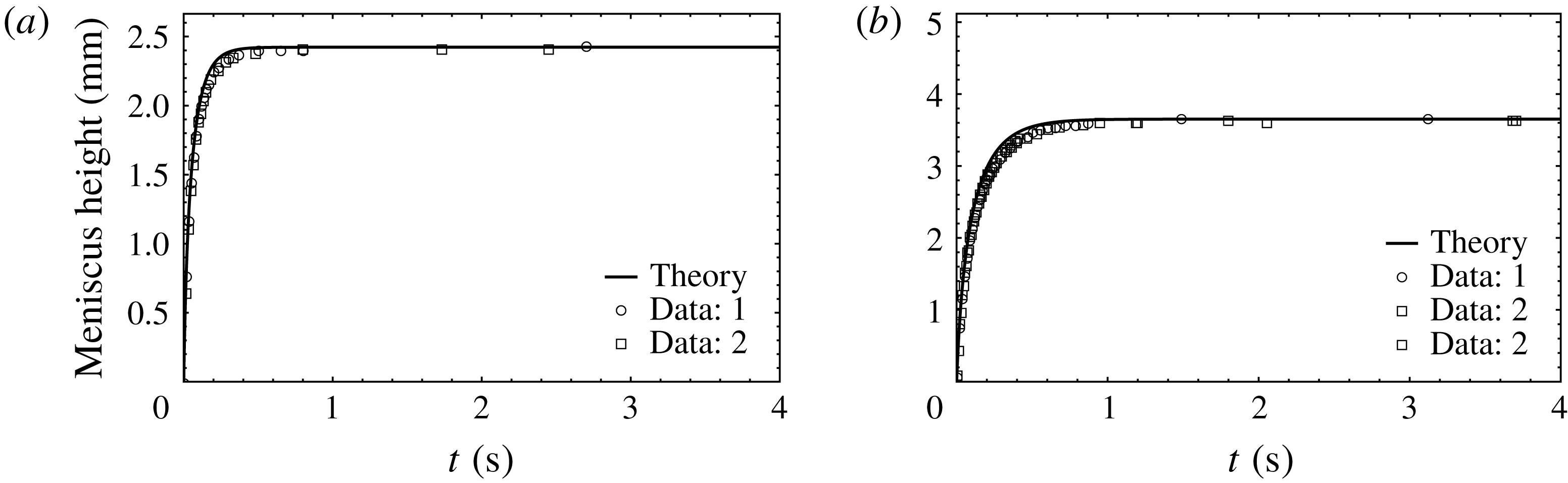
Figure 11. (a) Isocetane rise data for
 $L=400~\text{mm}$
and
$L=400~\text{mm}$
and
 $R=75~\unicode[STIX]{x03BC}\text{m}$
along with the theoretical prediction. The offset
$R=75~\unicode[STIX]{x03BC}\text{m}$
along with the theoretical prediction. The offset
 $z_{0}$
is
$z_{0}$
is
 $-0.123~\text{mm}$
,
$-0.123~\text{mm}$
,
 $H_{ec}$
is 2.45 mm and
$H_{ec}$
is 2.45 mm and
 ${\mathcal{S}}$
is 0.013. (b) Isocetane rise data for
${\mathcal{S}}$
is 0.013. (b) Isocetane rise data for
 $L=610~\text{mm}$
and
$L=610~\text{mm}$
and
 $R=75~\unicode[STIX]{x03BC}\text{m}$
and theory.
$R=75~\unicode[STIX]{x03BC}\text{m}$
and theory.
 $H_{ec}$
is 3.68 mm,
$H_{ec}$
is 3.68 mm,
 $z_{0}$
is
$z_{0}$
is
 $-0.136~\text{mm}$
, and
$-0.136~\text{mm}$
, and
 ${\mathcal{S}}$
is 0.011.
${\mathcal{S}}$
is 0.011.
6 Conclusions
Universal models that predict capillary rise dynamics across a range of capillary lengths and radii have been presented. With a self-consistent formulation, using results from single-phase hybrid-capillary flow, we address entry and exit effects, and inner and outer menisci movement. For the entry problem, the added mass inertia within the container consists of two distinct parts: (i) acceleration of the container fluid due to flow into the capillary and (ii) acceleration of the fluid due to the presence of an outer meniscus. The latter appears necessary for capturing time periods correctly.
For gas flow, the closed-capillary problem requires multiple length and time scales. New results for capillary rise based on a perturbation solution for laminar flow for gas with moving and sealed boundary conditions have been derived. The resulting perturbation solution, when included in the rise formulation, agrees with data in closed capillaries for three different liquids over a range of capillary sizes.
Corrections from a static contact angle to a dynamic one with a fixed
 $\unicode[STIX]{x1D6FD}$
appear to be adequate for the liquids studied. Hysteresis models fit the data no better than a single
$\unicode[STIX]{x1D6FD}$
appear to be adequate for the liquids studied. Hysteresis models fit the data no better than a single
 $\unicode[STIX]{x1D6FD}$
value. In general,
$\unicode[STIX]{x1D6FD}$
value. In general,
 $\unicode[STIX]{x1D6FD}$
decreases amplitude of oscillation or entirely suppresses it. While the moving contact line problem is virtually intractable in its fine details, the macroscopic rise dynamics given in this paper seems sufficient.
$\unicode[STIX]{x1D6FD}$
decreases amplitude of oscillation or entirely suppresses it. While the moving contact line problem is virtually intractable in its fine details, the macroscopic rise dynamics given in this paper seems sufficient.
Appendix A. Entry loss
Capillary rise dynamics is a complex moving contact line problem, and is difficult due to the rearrangement of streamlines near the moving interface to accommodate uniform velocity. The additional friction of the ordered structure at the interface contact line is taken into account through
 $\unicode[STIX]{x1D6FD}$
, but here our aim is to infer entry loss due to flow into a capillary from a container and the streamlines rearrangement. In dimensionless form, this should be a function of Reynolds number,
$\unicode[STIX]{x1D6FD}$
, but here our aim is to infer entry loss due to flow into a capillary from a container and the streamlines rearrangement. In dimensionless form, this should be a function of Reynolds number,
 $\mathfrak{R}\mathfrak{e}_{l}$
, and
$\mathfrak{R}\mathfrak{e}_{l}$
, and
 $h_{e}/R$
, for a sufficiently large container size. Pressure loss for the rising liquid corresponds to
$h_{e}/R$
, for a sufficiently large container size. Pressure loss for the rising liquid corresponds to
 ${\mathcal{L}}_{frl}$
. Gas retracts during liquid rise and this is addressed as a part of exit loss in appendix B. Pressure loss during gas entry is labelled
${\mathcal{L}}_{frl}$
. Gas retracts during liquid rise and this is addressed as a part of exit loss in appendix B. Pressure loss during gas entry is labelled
 ${\mathcal{L}}_{frg}$
and its functional form is the same as
${\mathcal{L}}_{frg}$
and its functional form is the same as
 ${\mathcal{L}}_{frl}$
, except that
${\mathcal{L}}_{frl}$
, except that
 $\mathfrak{R}\mathfrak{e}_{l}$
should be replaced by
$\mathfrak{R}\mathfrak{e}_{l}$
should be replaced by
 $\mathfrak{R}\mathfrak{e}_{g}$
in the argument.
$\mathfrak{R}\mathfrak{e}_{g}$
in the argument.
For a quantitative estimate of
 ${\mathcal{L}}_{frl}$
, we set a capillary of length of
${\mathcal{L}}_{frl}$
, we set a capillary of length of
 $h_{e}$
along which a no-slip boundary condition is satisfied. In the dynamic problem,
$h_{e}$
along which a no-slip boundary condition is satisfied. In the dynamic problem,
 $h_{e}$
varies with
$h_{e}$
varies with
 $t$
. Since computing
$t$
. Since computing
 ${\mathcal{L}}_{frl}$
is based on steady single-phase flow,
${\mathcal{L}}_{frl}$
is based on steady single-phase flow,
 $h_{e}$
is fixed for numerical simulation; therefore, the computation is rapid. We add a suitable length
$h_{e}$
is fixed for numerical simulation; therefore, the computation is rapid. We add a suitable length
 $L-h_{e}$
of capillary of the same radius
$L-h_{e}$
of capillary of the same radius
 $R$
, on the surface of which, the liquid has perfect slip.
$R$
, on the surface of which, the liquid has perfect slip.
 $L$
is large enough that capillary outlet velocity is uniform. Thus pressure recovery due to rearrangement from a parabolic profile to a plug-flow profile is automatically included. At the outlet, pressure is at 0 Pa whereas the side and bottom boundaries of the container are kept at an elevated pressure to cause flow through the capillary. Note that this is with incompressible flow and therefore the datum pressure is arbitrary. The elevated pressure fixes the flow rate. Once the velocity through the capillary is numerically evaluated,
$L$
is large enough that capillary outlet velocity is uniform. Thus pressure recovery due to rearrangement from a parabolic profile to a plug-flow profile is automatically included. At the outlet, pressure is at 0 Pa whereas the side and bottom boundaries of the container are kept at an elevated pressure to cause flow through the capillary. Note that this is with incompressible flow and therefore the datum pressure is arbitrary. The elevated pressure fixes the flow rate. Once the velocity through the capillary is numerically evaluated,
 $\mathfrak{R}\mathfrak{e}_{l}$
is known. We used COMSOL (trademark of COMSOL Inc.) to carry out these calculations over a range of
$\mathfrak{R}\mathfrak{e}_{l}$
is known. We used COMSOL (trademark of COMSOL Inc.) to carry out these calculations over a range of
 $h_{e}$
and
$h_{e}$
and
 $R$
.
$R$
.
The boundary value problem satisfies continuity, i.e.
 $\unicode[STIX]{x1D735}\boldsymbol{\cdot }\boldsymbol{v}=0$
, and the Navier–Stokes equation in
$\unicode[STIX]{x1D735}\boldsymbol{\cdot }\boldsymbol{v}=0$
, and the Navier–Stokes equation in
 $(r,z)$
(Bird, Stewart & Lightfoot Reference Bird, Stewart and Lightfoot2002). We impose
$(r,z)$
(Bird, Stewart & Lightfoot Reference Bird, Stewart and Lightfoot2002). We impose
 $p=P_{f}$
as
$p=P_{f}$
as
 $r\rightarrow \infty$
and
$r\rightarrow \infty$
and
 $z\rightarrow -\infty$
in the container. Also
$z\rightarrow -\infty$
in the container. Also
 $p=P_{0}=0$
at
$p=P_{0}=0$
at
 $z=L+z_{r}$
and
$z=L+z_{r}$
and
 $0\leqslant r\leqslant R$
, i.e. at the capillary top. At the surface of the container, i.e.
$0\leqslant r\leqslant R$
, i.e. at the capillary top. At the surface of the container, i.e.
 $R\leqslant \infty$
,
$R\leqslant \infty$
,
 $z=z_{r}$
, shear stress is zero to mimic the liquid–air interface. In the no-slip length of the capillary of height
$z=z_{r}$
, shear stress is zero to mimic the liquid–air interface. In the no-slip length of the capillary of height
 $h_{e}$
,
$h_{e}$
,
 $\boldsymbol{v}=0$
at
$\boldsymbol{v}=0$
at
 $r=R$
. The slip section of the capillary has zero shear at the wall. Visualizing the boundary value problem follows from the results presented in this appendix and appendix B. The container is sufficiently large that its size plays little role in determining the losses. There is no need to consider gravity or body force in these calculations, because in single-phase flow
$r=R$
. The slip section of the capillary has zero shear at the wall. Visualizing the boundary value problem follows from the results presented in this appendix and appendix B. The container is sufficiently large that its size plays little role in determining the losses. There is no need to consider gravity or body force in these calculations, because in single-phase flow
 $P_{f}$
may be regarded as a drive potential. For each
$P_{f}$
may be regarded as a drive potential. For each
 $h_{e}$
, and for a given
$h_{e}$
, and for a given
 $P_{f}$
, simulation may be used to calculate the mass flow rate
$P_{f}$
, simulation may be used to calculate the mass flow rate
 $M$
. For this
$M$
. For this
 $M$
, we calculate average velocity from
$M$
, we calculate average velocity from
 $\hat{V}=M/(\unicode[STIX]{x03C0}R^{2}\unicode[STIX]{x1D70C})$
. Two different velocity maps, one with a drive of 10 Pa, and another with a drive of 1 Pa are shown in figure 12. As anticipated, a region of container having non-zero inertia must be considered for describing the moving meniscus. The shape of this region varies with
$\hat{V}=M/(\unicode[STIX]{x03C0}R^{2}\unicode[STIX]{x1D70C})$
. Two different velocity maps, one with a drive of 10 Pa, and another with a drive of 1 Pa are shown in figure 12. As anticipated, a region of container having non-zero inertia must be considered for describing the moving meniscus. The shape of this region varies with
 $\mathfrak{R}\mathfrak{e}_{l}$
, and a fixed added mass is inadequate.
$\mathfrak{R}\mathfrak{e}_{l}$
, and a fixed added mass is inadequate.

Figure 12. Axisymmetric velocity map on a rainbow scale for 10 Pa (a) and 1 Pa (b) drive from the periphery. The capillary is 1 mm radius. In (a)
 $\mathfrak{R}\mathfrak{e}_{l}\approx 75.5$
and is
$\mathfrak{R}\mathfrak{e}_{l}\approx 75.5$
and is
 ${\approx}9$
in (b). The no-slip/slip transition in the capillary is at
${\approx}9$
in (b). The no-slip/slip transition in the capillary is at
 $z-z_{r}$
of 20 mm. Notice the flow rearrangement to uniform profile past this length. Also, the entry region below the capillary is more hemispherical in (b), and its shape changes with
$z-z_{r}$
of 20 mm. Notice the flow rearrangement to uniform profile past this length. Also, the entry region below the capillary is more hemispherical in (b), and its shape changes with
 $\mathfrak{R}\mathfrak{e}_{l}$
. Since the pressure at the entry is different from
$\mathfrak{R}\mathfrak{e}_{l}$
. Since the pressure at the entry is different from
 $P_{f}-(1/2)\unicode[STIX]{x1D70C}_{l}\hat{V}^{2}$
and is not uniform, one has to account for flow losses outside and within the capillary. Maximum and minimum velocity magnitudes are above and below the colour bar and are shown with up and down triangles.
$P_{f}-(1/2)\unicode[STIX]{x1D70C}_{l}\hat{V}^{2}$
and is not uniform, one has to account for flow losses outside and within the capillary. Maximum and minimum velocity magnitudes are above and below the colour bar and are shown with up and down triangles.
In the absence of entry and flow rearrangement loss or gain, from the Bernoulli equation, and laminar-flow-induced loss on the capillary wall of length
 $h_{e}$
, since
$h_{e}$
, since
 $P_{0}=0~\text{Pa}$
,
$P_{0}=0~\text{Pa}$
,
 $$\begin{eqnarray}P_{f}=\frac{1}{2}\unicode[STIX]{x1D70C}_{l}\hat{V}^{2}+\frac{8\unicode[STIX]{x1D707}_{l}\hat{V}h_{e}}{R^{2}}\quad \text{for }{\mathcal{L}}_{frl}=0.\end{eqnarray}$$
Therefore, we calculate
 ${\mathcal{L}}_{frl}$
from
${\mathcal{L}}_{frl}$
from
 $$\begin{eqnarray}{\mathcal{L}}_{frl}=P_{f}-\frac{1}{2}\unicode[STIX]{x1D70C}_{l}\hat{V}^{2}-\frac{8\unicode[STIX]{x1D707}_{l}\hat{V}h_{e}}{R^{2}}.\end{eqnarray}$$
The dimensionless form of
 ${\mathcal{L}}_{frl}$
may be written as
${\mathcal{L}}_{frl}$
may be written as
 $$\begin{eqnarray}\frac{2{\mathcal{L}}_{frl}}{\unicode[STIX]{x1D70C}_{l}\hat{V}^{2}}=f_{r}\left(\mathfrak{R}\mathfrak{e}_{l};\frac{h_{e}}{R}\right),\end{eqnarray}$$
where
 $f_{r}$
is the function whose first argument is
$f_{r}$
is the function whose first argument is
 $\mathfrak{R}\mathfrak{e}_{l}$
for
$\mathfrak{R}\mathfrak{e}_{l}$
for
 ${\mathcal{L}}_{frl}$
and
${\mathcal{L}}_{frl}$
and
 $\mathfrak{R}\mathfrak{e}_{g}$
for gas entry; for the latter the value computed is for
$\mathfrak{R}\mathfrak{e}_{g}$
for gas entry; for the latter the value computed is for
 $2{\mathcal{L}}_{frg}/(\unicode[STIX]{x1D70C}_{g}\hat{V}^{2})$
. The values of
$2{\mathcal{L}}_{frg}/(\unicode[STIX]{x1D70C}_{g}\hat{V}^{2})$
. The values of
 ${\mathcal{L}}_{frl}$
over kinetic energy (per unit volume) are plotted with respect to
${\mathcal{L}}_{frl}$
over kinetic energy (per unit volume) are plotted with respect to
 $1/\mathfrak{R}\mathfrak{e}_{l}$
in figure 13. The various markers are for
$1/\mathfrak{R}\mathfrak{e}_{l}$
in figure 13. The various markers are for
 $h_{e}/(2R)$
of 0.25, 0.5, 1, 2.5, 5 and 10. Fortunately, for the accuracy desired in our predictive model, a correlation of the form
$h_{e}/(2R)$
of 0.25, 0.5, 1, 2.5, 5 and 10. Fortunately, for the accuracy desired in our predictive model, a correlation of the form
 $$\begin{eqnarray}f_{r}\left(\mathfrak{R}\mathfrak{e};\frac{h_{e}}{R}\right)\approx 0.54+27/\mathfrak{R}\mathfrak{e}\end{eqnarray}$$
is adequate. This is shown as the line fitted through the data points. The correlation applies for liquid entry with
 $\mathfrak{R}\mathfrak{e}=\mathfrak{R}\mathfrak{e}_{l}$
, and for gas entry from the top with
$\mathfrak{R}\mathfrak{e}=\mathfrak{R}\mathfrak{e}_{l}$
, and for gas entry from the top with
 $\mathfrak{R}\mathfrak{e}=\mathfrak{R}\mathfrak{e}_{g}$
.
$\mathfrak{R}\mathfrak{e}=\mathfrak{R}\mathfrak{e}_{g}$
.

Figure 13. (a) Simulation results translated to dimensionless loss in pressure as a function of
 $\mathfrak{R}\mathfrak{e}_{l}$
and
$\mathfrak{R}\mathfrak{e}_{l}$
and
 $h_{e}/R$
are shown;
$h_{e}/R$
are shown;
 $2{\mathcal{L}}_{fr}/(\unicode[STIX]{x1D70C}\hat{V}^{2})$
is approximately linear with respect to
$2{\mathcal{L}}_{fr}/(\unicode[STIX]{x1D70C}\hat{V}^{2})$
is approximately linear with respect to
 $1/\mathfrak{R}\mathfrak{e}$
. In (b)
$1/\mathfrak{R}\mathfrak{e}$
. In (b)
 $m_{R}/\unicode[STIX]{x1D70C}$
is shown to correlate to
$m_{R}/\unicode[STIX]{x1D70C}$
is shown to correlate to
 $\mathfrak{R}\mathfrak{e}$
for different
$\mathfrak{R}\mathfrak{e}$
for different
 $h_{e}/(2R)$
and for
$h_{e}/(2R)$
and for
 $P_{f}$
from 0.05 Pa to 50 Pa.
$P_{f}$
from 0.05 Pa to 50 Pa.
Along with the liquid rise calculation, we may also correlate (see figure 13
b)
 $m_{R}/\unicode[STIX]{x1D70C}_{l}$
to
$m_{R}/\unicode[STIX]{x1D70C}_{l}$
to
 $\mathfrak{R}\mathfrak{e}_{l}$
and
$\mathfrak{R}\mathfrak{e}_{l}$
and
 $h_{e}/R$
, by computing
$h_{e}/R$
, by computing
 $m_{R}$
through (3.6); this is needed for expressing the rate of change of momentum within the container with given external force or pressure. The same correlation may be applied for gas intrusion from the capillary top, by replacing
$m_{R}$
through (3.6); this is needed for expressing the rate of change of momentum within the container with given external force or pressure. The same correlation may be applied for gas intrusion from the capillary top, by replacing
 $\mathfrak{R}\mathfrak{e}_{l}$
with
$\mathfrak{R}\mathfrak{e}_{l}$
with
 $\mathfrak{R}\mathfrak{e}_{g}$
and
$\mathfrak{R}\mathfrak{e}_{g}$
and
 $\unicode[STIX]{x1D70C}_{l}$
with
$\unicode[STIX]{x1D70C}_{l}$
with
 $\unicode[STIX]{x1D70C}_{g}$
. Here
$\unicode[STIX]{x1D70C}_{g}$
. Here
 $h_{e}/R$
shows little influence. The lognormal functional form of the correlation is
$h_{e}/R$
shows little influence. The lognormal functional form of the correlation is
 $$\begin{eqnarray}\frac{m_{R}}{\unicode[STIX]{x1D70C}}=0.8144+0.5006\exp \left[-\frac{\ln 1/(2.68\mathfrak{R}\mathfrak{e})}{3.536}\right].\end{eqnarray}$$
Since
 $m_{R}$
changes with
$m_{R}$
changes with
 $\hat{V}$
, it is necessary to include
$\hat{V}$
, it is necessary to include
 $m_{R}^{\prime }$
terms in the formulation.
$m_{R}^{\prime }$
terms in the formulation.
Appendix B. Exit loss
For the exit problem, numerical simulations show that the capillary outlet is nearly at 0 Pa, the pressure at the container periphery. The momentum outflow is lost. Computed results are shown in figure 14: isobars in (a) and the velocity map in (b). The exit velocity profile resembles a developed parabolic profile; therefore the momentum outflow flux is
 $(4/3)\unicode[STIX]{x1D70C}_{l}\hat{V}^{2}$
, whereas the inflow is
$(4/3)\unicode[STIX]{x1D70C}_{l}\hat{V}^{2}$
, whereas the inflow is
 $\unicode[STIX]{x1D70C}_{l}\hat{V}^{2}$
. During retraction, the liquid column height is assumed to be large enough for Poiseuille flow to develop within the capillary and loss is computed as per (3.5).
$\unicode[STIX]{x1D70C}_{l}\hat{V}^{2}$
. During retraction, the liquid column height is assumed to be large enough for Poiseuille flow to develop within the capillary and loss is computed as per (3.5).
 $P_{f}$
is maintained at the top of the capillary. A perfect-slip capillary wall is placed in the top section, followed by a no-slip capillary of length
$P_{f}$
is maintained at the top of the capillary. A perfect-slip capillary wall is placed in the top section, followed by a no-slip capillary of length
 $h_{e}$
.
$h_{e}$
.

Figure 14. (a) Isobars for
 $P_{f}=25~\text{Pa}$
. The bottom of the capillary is close to 0 Pa, the pressure at the container periphery. The plot is axisymmteric. Values below 0.01 Pa and above 25.01 Pa are left white. Speckling is due to discretization and contouring. (b) Velocity map for a drive of 25 Pa. At exit, the velocity profile is non-uniform, nearly the same as the developed parabolic profile.
$P_{f}=25~\text{Pa}$
. The bottom of the capillary is close to 0 Pa, the pressure at the container periphery. The plot is axisymmteric. Values below 0.01 Pa and above 25.01 Pa are left white. Speckling is due to discretization and contouring. (b) Velocity map for a drive of 25 Pa. At exit, the velocity profile is non-uniform, nearly the same as the developed parabolic profile.
Numerical results for
 $2{\mathcal{L}}_{fel}/(\unicode[STIX]{x1D70C}_{l}\hat{V}^{2})$
are described by a function
$2{\mathcal{L}}_{fel}/(\unicode[STIX]{x1D70C}_{l}\hat{V}^{2})$
are described by a function
 $f_{e}(\mathfrak{R}\mathfrak{e}_{l};h_{e}/R)$
given by
$f_{e}(\mathfrak{R}\mathfrak{e}_{l};h_{e}/R)$
given by
 $$\begin{eqnarray}\frac{2{\mathcal{L}}_{fel}}{\unicode[STIX]{x1D70C}_{l}\hat{V}^{2}}=f_{e}(\mathfrak{R}\mathfrak{e}_{l};h_{e}/R)=1.07+\frac{2985-1.07}{1+(56.94\mathfrak{R}\mathfrak{e}_{l})^{1.185}}.\end{eqnarray}$$
Dependence on
 $h_{e}/R$
is quite weak. Dimensionless gas exit loss is also calculated using
$h_{e}/R$
is quite weak. Dimensionless gas exit loss is also calculated using
 $f_{e}$
, but with argument
$f_{e}$
, but with argument
 $\mathfrak{R}\mathfrak{e}_{g}$
. Here
$\mathfrak{R}\mathfrak{e}_{g}$
. Here
 $f_{e}(\mathfrak{R}\mathfrak{e}_{g};h_{e}/R)$
is the ratio of
$f_{e}(\mathfrak{R}\mathfrak{e}_{g};h_{e}/R)$
is the ratio of
 ${\mathcal{L}}_{feg}$
and
${\mathcal{L}}_{feg}$
and
 $(1/2)\unicode[STIX]{x1D70C}_{g}\hat{V}^{2}$
.
$(1/2)\unicode[STIX]{x1D70C}_{g}\hat{V}^{2}$
.


