


1. Introduction
High-pressure blast waves are present and important in many natural and industrial processes, such as rocket propulsion systems, aerial boosters and explosions. Particularly important for current industrial safety issues, the accidental initiation of shock waves, such as hydrogen explosions in a confinement building, can lead to a potential hazard due to devastating effects on human lives and subsequent damage to the integrity of buildings. For safer engineering applications, several shock- and blast-wave mitigation techniques are proposed. A water spray system is one of the possible techniques used inside industrial buildings or on offshore facilities to preserve the containment integrity in case of severe accidents (Foissac et al. Reference Foissac, Malet, Vetrano, Buchlin, Mimouni, Feuillebois and Simonin2011). The mitigation effects of a spray system are directly dependent on the spray dispersion topology, which can be much affected by the shock-wave propagation. The interaction between spray and shock wave is also important in reacting flows, such as in internal combustion engine systems, where the combustion properties are much affected by the liquid fuels. As reported by Gelfand (Reference Gelfand1996), compression waves can, under some circumstances, coalesce and generate shock waves in two-phase reactive flows.
In the past, there have been many theoretical and experimental studies investigating the physics of the interaction of droplets or solid particles/obstacles with shock waves (Carrier Reference Carrier1958; Rudinger Reference Rudinger1964; Olim et al. Reference Olim, Ben-Dor, Mond and Igra1990; Geng et al. Reference Geng, Van de Ven, Yu, Zhang and Grönig1994; Chaudhuri et al. Reference Chaudhuri, Hadjadj, Sadot and Glazer2012, Reference Chaudhuri, Hadjadj, Sadot and Ben-Dor2013; Balakrishnan & Bellan Reference Balakrishnan and Bellan2017; Mouronval et al. Reference Mouronval, Tie, Hadjadj and Moebs2019; Gai et al. Reference Gai, Thomine, Hadjadj and Kudriakov2020). Commonly, the particles are assumed to be at rest before they meet the shock at a given velocity. In terms of flow dynamics and after the passage of the shock, the shocked gas induces high-velocity flow, which accelerates the particles. On the other hand, the particles decelerate the post-shock gas and thus attenuate the shock intensity (Jourdan et al. Reference Jourdan, Biamino, Mariani, Blanchot, Daniel, Massoni, Houas, Tosello and Praguine2010, Reference Jourdan, Mariani, Houas, Chinnayya, Hadjadj, Del Prete, Haas, Rambert, Counilh and Faure2015; Britan et al. Reference Britan, Shapiro, Liverts, Ben-Dor, Chinnayya and Hadjadj2013; Del Prete et al. Reference Del Prete, Chinnayya, Domergue, Hadjadj and Haas2013). In the case of a water spray and for high gas velocity, a secondary liquid droplet atomization may be encountered under certain flow conditions (e.g. Weber number  $We > 12$), which leads to the formation of a fine droplet spray that enhances shock energy dissipation (Pilch & Erdman Reference Pilch and Erdman1987; Gelfand Reference Gelfand1996; Guildenbecher, Lopez-Rivera & Sojka Reference Guildenbecher, Lopez-Rivera and Sojka2009). The role of atomization processes is thus to increase the transfer surface (Yeom & Chang Reference Yeom and Chang2012) and to intensify the heat (evaporation) as well as the mass transfer. These transfer processes largely affect the thermal equilibrium conditions of the post-shock gas (Kersey, Loth & Lankford Reference Kersey, Loth and Lankford2010) and may change the topology of the cloud dispersion, leading to shock-wave mitigation and/or a flame extinction in the case of reacting flows (Thomas Reference Thomas2000; Gai et al. Reference Gai, Kudriakov, Hadjadj, Studer and Thomine2019).
The physical mechanism of shock–droplets interaction is yet to be elucidated both quantitatively and qualitatively by means of well-conducted experiments and/or numerical modelling for low- and high-Mach-number regimes (Sugiyama et al. Reference Sugiyama, Ando, Shimura and Matsuo2019). Considering the complexity of droplet deformation, evaporation and the breakup mechanisms, rigid particles are easier to handle from the experimental viewpoint and simpler to model from the numerical side. The basic concept of the interactions between a shock wave and a single particle or an array of particles has been much discussed in the recent literature (Ling, Haselbacher & Balachandar Reference Ling, Haselbacher and Balachandar2011; Mehta et al. Reference Mehta, Jackson, Zhang and Balachandar2016; Dahal & McFarland Reference Dahal and McFarland2017), where the effects of particles on the gas flow are weak. Dense particles or droplet curtains have also been investigated (Wagner et al. Reference Wagner, Beresh, Kearney, Trott, Castaneda, Pruett and Baer2012; Theofanous, Mitkin & Chang Reference Theofanous, Mitkin and Chang2016) in which the collision between the particles becomes important.
In this study, we focus on the problem of shock waves interacting with particles having a volume fraction of the order of  ${O}(10^{-4}\text {--}10^{-3})$, which are typical values for the sprays found in industry. According to Elghobashi (Reference Elghobashi2006), a two-way formalism, which accounts for the mutual interaction between the gas flow and the droplets, can be used in such a case to describe the shock–spray interaction, meaning that the deceleration effects of the particles on the gas flow have to be taken into account, while the collisions between particles can be neglected.
From a practical point of view, concerning the modelling of an industrial building, the current existing numerical simulations cannot be applied directly as a result of high computational expense, especially for the simulation of high-Reynolds-number flows. By the necessity to develop a simple model, this paper presents a new methodology for modelling a shock wave propagating into spray droplets. The objective is twofold: (i) developing a reduced-order model of spray dispersion in the presence of shock waves taking into account the two-way interaction; and (ii) better understanding the different regimes of reflected pressure waves for both weak- and strong-Mach-number cases. From the highly resolved numerical simulation results, several fundamental hypotheses can be deduced for the shock–spray interaction. The reduced-order model is established by conservation laws, then validated through numerical simulations. The formation of the compressed gas zone is particularly discussed and a number-density peak of cloud particles is predicted, which is also seen in the highly resolved numerical simulations.
2. Modelling assumptions
In general, the following assumptions and simplifications are made in the numerical simulations: (i) The gas is considered as inviscid and obeys the perfect-gas law, and the fluid viscosity and conductivity are neglected except in the interaction with the particles. (ii) The particles are considered as inert, spherical, rigid and of uniform diameter, with constant heat capacity and a uniform temperature distribution. (iii) The volume fraction of the particles is taken to be small so that collisions between particles can be neglected, while the two-way shock–particles interaction is considered (Elghobashi Reference Elghobashi2006). (iv) Only the viscous drag forces are supposed to act on the particles. The particle-to-gas density ratio is assumed to be of the order of  ${O}(10^3)$, the Basset force can be neglected (Thomine Reference Thomine2011) and we assume that the particles do not spin (the Magnus force is neglected). Gravity is at least one order of magnitude smaller than the drag force for the range of parameters in this study, and therefore it is neglected. (v) Heat transfer between gas and particles is not considered at present for the dilute, homogeneous cloud of particles (Theofanous, Mitkin & Chang Reference Theofanous, Mitkin and Chang2018). (vi) Finally, the turbulent fluctuations of the solid particles are neglected in the one-dimensional configuration.
3. Governing equations
The structure of the shock–spray interaction is elucidated through direct numerical simulations carried out with a Navier–Stokes solver, named Asphodele, developed in CORIA Rouen to simulate two-phase dispersed fluid flows (Thomine Reference Thomine2011). The Eulerian–Lagrangian approach is used with an unresolved discrete particle model (UDPM), which relies on a larger computation cell with regard to the particle sizes and uses a drag force model to describe the gas–particle interactions. The space discretization uses a fifth-order weighted essentially non-oscillatory (WENO) scheme of Jiang & Shu (Reference Jiang and Shu1996) with a global Lax–Friedrichs splitting, and the time resolution employs a third-order Runge–Kutta method, with a minimal storage time-advancement scheme of Wray (Reference Wray1991).
In the Eulerian–Lagrangian frame, the mass, momentum and energy equations for the carrier gas phase can be written as:
 \begin{gather} \frac{\partial \rho_g}{\partial t} + \frac{\partial}{\partial x}(\rho_g u_g) = 0 {,} \end{gather}
 \begin{gather}\frac{\partial}{\partial t}(\rho_g u_g) + \frac{\partial}{\partial x}(\rho_g u_g^2+p) = -\boldsymbol{f}_D {,} \end{gather}
 \begin{gather}\frac{\partial}{\partial t}(\rho_g E_g) + \frac{\partial}{\partial x}(\rho_gH_gu_g) = -u_g\,\boldsymbol{f}_D {,} \end{gather}
with
 \begin{equation} \boldsymbol{f}_D = \frac{3}{4D}C_D\tau_{v}\rho_g |u_g - v_p | (u_g - v_p ) {,} \end{equation}
where the subscripts  $g$ and
  $p$ represent the gas and particle phases,
  $\tau _v$ denotes the particle volume fraction,
  $H_g$ is the specific total enthalpy of air,
  $u$ and
  $v$ represent the air and particle velocities,
  $C_D$ is the drag coefficient defined as
 \begin{equation} C_D = \frac{24}{Re_p} (1+0.15Re_p^{0.687} ) \quad \mbox{with}\ Re_p = \frac{\rho_g |u_g - v_p| D}{\mu_g} {,} \end{equation}
 $Re_p$ is the particle Reynolds number,
  $\mu _g$ is the dynamic viscosity of the gas and
  $D$ is the diameter of the particles.
For a solid particle, the general motion equation gives
 \begin{equation} m_p \frac{\textrm{d} V(t)}{\textrm{d} t} = \boldsymbol{F}_D = \frac{{\rm \pi} D^3}{6\tau_v} \, \boldsymbol{f}_D {,} \end{equation}
where  $m_p = {\rm \pi}\rho _p D^3/6$ is the particle mass,
  $\rho _p$ is the particle density and
  $\boldsymbol {F}_D$ is the drag force on the particle.
Conventionally, the unsteady terms of the gas–particle interaction, such as the added-mass effect and unsteady viscous force, are neglected for the conditions addressed, as a result of the high particle–gas density ratio  $\rho _p/\rho _f={O}(10^3)$ and the low particle volume fraction
  $\tau _{v,0}={O}(10^{-4})$ in the highly dilute homogeneous gas-cloud system (Ling, Parmar & Balachandar Reference Ling, Parmar and Balachandar2013; Theofanous & Chang Reference Theofanous and Chang2017). In this study, we mainly focus on the dynamic aspect of the shock–particle interaction. The heat transfer between the particle cloud and the gas flow may indirectly influence the gas and particle motion. However, this effect is considered to be of secondary importance for the development of the one-dimensional analytical model (Ling et al. Reference Ling, Wagner, Beresh, Kearney and Balachandar2012). The drag law is reported to yield good agreements with the dispersive behaviour found in experiments of one-dimensional shock–particle cloud interactions (Theofanous et al. Reference Theofanous, Mitkin and Chang2018). The turbulent dispersion of the particle cloud is not considered during the shock passage.
4. Interaction mechanism
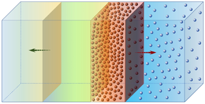
In this study, we consider the problem of the interaction between a planar shock wave and a gas–particle two-phase mixture, as illustrated in figure 1(a). This test problem represents one of the basic configurations commonly used to study shock-wave attenuation in multiphase flows (Chang & Kailasanath Reference Chang and Kailasanath2003). A wave travelling at velocity  $V_s$ in a shock tube of constant cross-sectional area is generated by a piston moving at a speed
  $u_{g,1}$. After the passage of the wave, four states can be distinguished: (1) the pure gas, (2) the compressed gas, (3) the post-shock gas–particle mixture and (4) the pre-shock gas–particle mixture. Let
  $M_s = V_s/c_0$ (with
  $c_0$ being the speed of sound in the unshocked gas region) denote the incident shock Mach number. For a low-velocity impact, i.e. weak Mach number (
 $M_s<2$), the incident shock generates a transmitted wave and a reflected left-running pressure wave with respect to the incident shock (see figure 1b). The gas–particle contact surface moves with the transmitted shock at velocity
  $V_i$. For stronger incident Mach number, the reflected pressure expansion is seen to propagate along the original shock-propagation direction as shown in figure 1(c).

Figure 1. Sketch of the two regimes of shock–particle cloud interaction: (a) initial configuration; (b) weak Mach number  $M_s<2$; and (c) strong Mach number
  $M_s>2$. Here CG = compressed gas, and P = particles.
Space–time diagrams are plotted for the two different regimes of shock reflection, as seen in figures 2(a) and 2(b). The propagation direction of the pressure expansion is closely related to the properties of the compressed gas region. For simplicity, the properties are denoted with the indices of the corresponding area as presented in figure 1. The spherical particles are assumed to have a volume fraction of  $\tau _{v,0}=\mathcal {V}_p/(\mathcal {V}_p + \mathcal {V}_g)=5.2\times 10^{-4}$, where
  $\mathcal {V}_p$ and
  $\mathcal {V}_g$ are the volume of particles and the volume of gas, respectively.

Figure 2. Space–time diagrams of shock–particles interaction for numerical simulations at two different Mach numbers: (a)  $M_s = 1.1$ and (b)
  $M_s = 4.0$. Curves: transmitted wave (blue-green dot-dashed); reflected wave (blue dotted); particle interface (red solid); and initial particle interface (orange dashed).
Particles with a mean diameter of  $1\ \mathrm {\mu } \textrm {m}$ are used in the numerical simulations to investigate the shock–spray interaction mechanism, since they have a small characteristic response time
  $\tau _p$. Figure 3 gives a space distribution of gas density
  $\rho _g$ (figure 3a) and velocity
  $u_g$ (figure 3b) at a given time. One can identify the different zones of the interaction as well as the two regimes of shock reflection for weak- and strong-Mach-number cases as described in figure 1. In what follows we will derive the relationships between pressure, gas density and velocity. These observations will contribute to the development of the reduced-order modelling approach.

Figure 3. Evolution of (a) gas mass density  $\rho _g$, (b) gas velocity
  $u_g$, (c) particle volume fraction
  $\tau _v$ and (d) particle mean velocity
  $v_p$ for numerical simulations, at
  $t = 300\ \mathrm {\mu } \textrm {s}$,
  $D = 1\ \mathrm {\mu } \textrm {m}$ and
  $\tau _{v,0}=5.2\times 10^{-4}$, for different Mach numbers. Curves:
  $M_s = 1.5$ (blue-green);
  $M_s = 2.0$ (blue);
  $M_s = 2.5$ (red); and original gas–particle contact surface (black dashed).
4.1. Pressure and density relationships in the compressed gas
To better represent the quantities in different zones, the gas density and velocity evolutions in figures 3(a) and 3(b) are sketched in figure 4. The evolutions of the particle volume fraction and the particle mean density are shown in figures 3(c) and 3(d). As illustrated in figure 1(b) and (c), after the interaction of the shock with the gas–particle contact surface, a compressed gas zone (2) is generated. From a modelling point of view, it is important to derive relationships between the pure gas zone (1) and the compressed gas zone (2), as follows:
 \begin{equation} p_{g,1} < p_{g,2}, \quad \rho_{g,1} < \rho_{g,2}, \quad u_{g,1} > u_{g,2}. \end{equation}
Similarly, between the compressed gas zone (2) and the post-shock gas–particle mixture (3), one has the following:
 \begin{equation} p_{g,2} = p_{g,3}, \quad \rho_{g,2} > \rho_{g,3} \quad u_{g,2} = u_{g,3}. \end{equation}
Figure 4. Sketch of gas properties after the shock–particle cloud interaction: (a) density and (b) gas velocity evolutions.
With regard to the gas density distribution, and as depicted in figure 4(a), the gas density inside the post-shock gas–particle mixture  $\rho _{g,3}$ might be higher than, lower than or equal to the density of the pure gas zone
  $\rho _{g,1}$. One can use
  $\rho _{g,3l}$,
  $\rho _{g,3c}$ and
  $\rho _{g,3r}$ to denote the three different cases. The numerical results show that, when one has
  $\rho _{g,1}<\rho _{g,3l}$ (for weak
  $M_s$), the reflected pressure expansion tends to propagate towards the
  $x^-$ direction, while if
  $\rho _{g,1}>\rho _{g,3r}$ (for strong
  $M_s$), the pressure expansion propagates inversely for most numerical simulations.
The gas velocity evolution, described in figure 4(b), indicates that, during the interaction, one always has  $u_{g,1}>u_{g,2}$,
  $u_{g,2} = u_{g,3}$ and
  $u_{g,3}>u_{g,4}=0$. It is interesting to note that, for a wide range of particle volume fractions (
 $\tau _{v,0}\approx {O}(10^{-5}\text {--}10^{-3})$), the velocity ratio in the pure and in the compressed gas regions is almost constant over a wide range of Mach numbers (
 $1<M_s<4$) (see figure 5). We assume therefore that
 \begin{equation} \frac{u_{g,2}}{u_{g,1}}\approx f(\tau_{v,0}), \end{equation}
where  $\tau _{v,0}$ is the initial particle volume fraction, which is considered to be the main factor influencing the variation of
  $u_{g,2}/u_{g,1}$. Equations (4.1a–c) to (4.3) are considered as the fundamental hypothesis of the reduced-order modelling.

Figure 5. Velocity ratio  $u_{g,2}/u_{g,1}$ over a wide range of incident shock Mach numbers, for
  $D = 1\ \mathrm {\mu } \textrm {m}$ and:
  $\tau _{v,0} = 5.2\times 10^{-5}$ (green),
  $\tau _{v,0} = 5.2\times 10^{-4}$ (blue) and
  $\tau _{v,0} = 5.2\times 10^{-3}$ (blue-green).
5. Reduced-order modelling
For practical applications, the development of a reduced-order model that takes into consideration the two-way shock–spray interaction is given in this section. The rationality of the above-mentioned hypotheses is discussed and the validation of the model is carried out with the Navier–Stokes (NS) code.
Mass conservation through the interface between the pure gas (1) and the compressed gas (2) gives
 \begin{equation} \int_{x_1}^{x_2}\left( \frac{\partial \rho_g}{\partial t} \right)\textrm{d}x= \rho_{g,1} u_{g,1} - \rho_{g,2} u_{g,2}, \end{equation}
where the integral expression on the left-hand side provides the direction of the pressure expansion. The pressure wave propagates towards the  $x^+$ direction if the integral is negative and vice versa. Thus the quantity (
 $\rho _{g,1}u_{g,1} - \rho _{g,2}u_{g,2}$) can be used as a criterion for the identification of the reflection regime of the pressure wave. This criterion is valid for cases corresponding to the initial configuration given in figure 1(a).
The properties of the pure gas zone (1) can be obtained analytically (White Reference White2011):
 \begin{gather} \frac{2}{\gamma+1} \frac{M_s^2 - 1}{M_s} = \frac{u_{g,1}}{c_0}, \end{gather}
 \begin{gather}\frac{p_1}{p_0} = \mathcal{F}_1(M_s,\gamma){,} \quad \frac{T_1}{T_0} = \frac{\mathcal{F}_1(M_s,\gamma)\,\mathcal{F}_2(M_s,\gamma)}{M_s^2}{,} \quad \frac{\rho_1}{\rho_0} = \frac{p_1}{p_0} \frac{T_0}{T_1} {,} \end{gather}
where
 \begin{align} \mathcal{F}_1(M_s,\gamma) = \frac{2}{\gamma+1} \left ( \gamma M_s^2 - \frac{\gamma-1}{2} \right ) {,} \quad \mathcal{F}_2(M_s,\gamma) = \frac{2}{\gamma+1} \left ( 1+\frac{\gamma-1}{2} M_s^2 \right ) {.} \end{align}
Note that the gas properties in the gas–particle mixture (4) are identical to those of the pre-shock pure gas area (0). Meanwhile, the gas properties in zones (2) and (3) need to be estimated properly.
5.1. Velocity of the compressed gas
It is noted from various numerical simulations that, for weak initial Mach numbers, the reflected pressure expansion has the velocity of the sound speed in zone (1). Here we consider the particular case where  $\rho _{g,1}=\rho _{g,3c}$, as illustrated in figure 4(a). In this case, the interface between zone (1) and zone (2) remains stationary in the laboratory frame, which can be characterized by
  $u_{g,1} = c_1= \sqrt {{\gamma p_1}/{\rho _{g,1}}}$, with
  $c_1$ being the sound speed in zone (1). Using the gas properties across the shock wave (White Reference White2011), one can deduce that
 \begin{equation} c_0\frac{2}{\gamma+1} \frac{M_s^2 - 1}{M_s} = \sqrt{\frac{\gamma p_1}{\rho_{g,1}}}, \end{equation}
which can be simplified to
 \begin{equation} (M_s^2-1)^2 = \left(\frac{\gamma + 1}{2}\right)^2 \mathcal{F}_1(M_s,\gamma)\, \mathcal{F}_2(M_s,\gamma). \end{equation}
 The Mach number that satisfies (5.6) is known as the critical Mach number, and is  $M_{s,cr} = 2.0$ for a monatomic ideal gas (
 $\gamma = 7/5$). The results of figure 3(a) show that
  $\rho _{g,3}=\rho _{g,1}$ and
  $u_{g,3}=u_{g,2}$ when
  $M_s=M_{s,cr}$. The conservation of kinetic energy before and after the passage of the shock gives
 \begin{equation} \rho_{g,1}u_{g,1}^2 = \tau_{v,0}\rho_p{u}_{g,3}^2 + (1-\tau_{v,0})\rho_{g,3}{u}_{g,3}^2, \end{equation}
where  ${u}_{g,3}$ is the velocity of the shocked gas in the gas–particle mixture and
  $\rho _p$ is the mass density of the particles. By combining (4.3) and (5.7), the estimate of
  $u_{g,2}$ can be obtained for a given
  $\tau _{v,0}$ as
 \begin{equation} \frac{{u}_{g,2}}{u_{g,1}} \approx \left(\frac{{u}_{g,2}}{u_{g,1}}\right)_{cr} = \sqrt{\frac{1}{1-\tau_{v,0}+\tau_{v,0}\dfrac{\rho_p}{\rho_{g,1}}}}. \end{equation}
5.2. Density of the compressed gas
To estimate the density of the compressed gas  $\rho _{g,2}$, one can assume that the pressure wave reflection process obeys an isentropic expansion. The isentropic hypothesis is discussed in appendix A. The conservation of momentum leads to
 \begin{equation} \rho_{g,2}u_{g,2}^2 + p_1\left(\frac{\rho_{g,2}}{\rho_{g,1}} \right)^\gamma = \rho_{g,1}u_{g,1}^2 + p_1. \end{equation}
For a given estimated  $u_{g,2}$, the solution of (5.9) can provide an estimate of
  $\rho _{g,2}$. A Newton–Raphson method is used to solve (5.9).
The estimate of  $\rho _{g,2}$ can also contribute to the evaluation of the intensity of the pressure expansion. Moreover, knowing the two properties of the flow,
  $u_{g,2}$ and
  $\rho _{g,2}$, one can easily predict the propagation direction of the pressure expansion after the interaction of the shock with the spray by using the criterion given by (5.1).
5.3. Spray dispersion
Equation (5.7) can also be applied to estimate the particle dispersion in the post-shock gas–particle mixture (3). Figure 6 shows the configuration in the proximity of the transmitted shock inside the gas–particle zone in the shock-attached frame, where the properties across the transmitted shock wave are depicted in figure 6. One knows that
 \begin{equation} {p}_3={p}_2, \quad {u}_{g,3}= {u}_{g,2}, \quad u_{g,4} = 0, \end{equation}
where  ${u}_{g,3}$ and
  ${u}_{g,2}$ are estimated quantities. Thus, the conservation of mass across the shock wave gives
 \begin{equation} {\rho}_{g,3} (V_s- {u}_{g,2}) = {\rho}_{g,4}V_s. \end{equation}
Figure 6. Sketch of the shock front transmitted into the gas–particle zone in the shock-attached frame. Here CG = compressed gas, P = particles, and G = unshocked gas.
Taking into account the initial volume fraction  $\tau _{v,0}$ of particles, the conservation of momentum gives
 \begin{align} p_2 + {\rho}_{g,3}(1-\tau_v)(V_s- {u}_{g,2})^2 + \rho_p\tau_v(V_s- {u}_{g,2})^2 = p_4 + {\rho}_{g,4}(1-\tau_{v,0})V_s^2 +\rho_p\tau_{v,0}V_s^2, \end{align}
where  $\tau _v$ is the volume fraction of the particles in the post-shock region (3). Before the shock passage, the initial cloud length is
  $V_s t$ and becomes
  $(V_s - {u}_{g,2} ) t$ afterwards. Therefore, the post-shock volume fraction of the particles
  ${\tau _v}$ can be linked to the pre-shock volume fraction
  $\tau _{v,0}$ through
 \begin{equation} {\tau_v} = \tau_{v,0} \,\frac{V_s}{V_s - {u}_{g,2}} {.} \end{equation}
By combining (5.11)–(5.13), one can deduce an analytical expression for the velocity of the transmitted shock wave  $V_s$:
 \begin{equation} V_s = \frac{p_2 - p_4}{(\rho_{g,4}+\rho_p\tau_{v,0}) {u}_{g,2}}. \end{equation}
Knowing  $V_s$, the volume fraction of the particles in region (3) can be calculated by (5.13).
5.4. Assessment of the reduced-order model
From the above discussion, the modelling is achieved for  $u_{g,2}$,
  $\rho _{g,2}$,
  $p_2$ and
  $\tau _v$, for a given initial volume fraction
  $\tau _{v,0}$ and incident Mach number
  $M_s$. The estimates of
  $\rho _{g,2}$ and
  $\tau _v$ rely especially on the accuracy of
  $u_{g,2}$. However, the post-shock maximal particle volume fraction has similar values for particles of different diameters. The maximal volume fractions of small particles can provide guideline values for the larger ones. The assessment of the proposed model, especially for the estimation of
  $u_{g,2}$,
  $\rho _{g,2}$ and
  $\tau _v$, is achieved through a direct comparison with the results from the NS solver.
Taking an example of the initial particle volume fraction  $\tau _{v,0} = 5.2\times 10^{-4}$, in critical conditions, in which
  $\rho _{g,3c} = \rho _{g,1}$, the velocity ratio calculated by the NS code is
  $u_{g,2}/u_{g,1}=0.9$, and (5.7) gives a ratio of
  $0.93$. If the gas velocity
  $u_{g,2}$ in the compressed zone is correctly estimated, the model evaluations for
  $\rho _{g,2}$ and
  $p_2$ are in good agreement with the numerical simulations, as shown in figure 7(a–d). For
  $\tau _{v,0} = 5.2\times 10^{-4}$ and
  $M_s = 2.0$, the density estimated by (5.9) is
  $\rho _{g,2} = 3.4\ \textrm {kg}\,\textrm {m}^{-3}$, and the value calculated by the NS code is
  $\rho _{g,2} = 3.44\ \textrm {kg}\,\textrm {m}^{-3}$.

Figure 7. Evolution of different flow properties as a function of  $M_s$: (a) gas velocity, (b) gas density, (c) gas pressure and (d) particle volume fraction. Simulation using NS code:
  $\tau _{v,0} =5.2\times 10^{-3}$ (yellow dot-dashed);
  $\tau _{v,0} =5.2\times 10^{-4}$ (red dashed); and
  $\tau _{v,0} =5.2\times 10^{-5}$ (blue-green dotted). Current model:
  $\tau _{v,0} =5.2\times 10^{-3}$ (inverted triangles);
  $\tau _{v,0} =5.2\times 10^{-4}$ (circles); and
  $\tau _{v,0} =5.2\times 10^{-5}$ (triangles).
For the ratio of the particle volume fraction  $\tau _v/\tau _{v,0}$, using (5.13), one can have higher relative differences compared to the numerical simulation, since the estimation of this ratio is based on the modelling of both
  $u_{g,2}$ and
  $\rho _{g,2}$. In the case where these two parameters have a relative difference of
  $5\,\%$, one may have a relative difference of
  $28\,\%$ for
  $\tau _v/\tau _{v,0}$ as a result of the difference accumulation, as shown in figure 7(d).
The analytical model is assessed in this study by the NS solver for the interaction between supersonic flows of Mach number  $M_s=1.1\text {--}4$ and a particle cloud of volume fraction
  $\tau _{v,0}=10^{-5}\text {--}10^{-3}$ and of particle diameters
  $D=1\text {--}10\ \mathrm {\mu } \textrm {m}$. For shock waves of Mach number higher than
  $M_s=5$, the heat transfer induced by the hypersonic shock should be considered. The present model can be applied to solid particles or liquid droplets having relatively high surface tension values. For higher volume fraction
  $\tau _{v,0} > 10^{-3}$ of particle clouds, the interactions among the particles become important, such as particle collision and coalescence of droplets, as noted by Elghobashi (Reference Elghobashi1994). For water droplets of diameter larger than
  $D > 10\ \mathrm {\mu } \textrm {m}$, the breakup of the droplets in high-velocity gas flow becomes important. Particles of diameter
  ${O}(10\ \mathrm {\mu } \textrm {m})$ can be regarded as stable fragments of larger droplets according to Pilch & Erdman (Reference Pilch and Erdman1987).
5.5. Influence of the particle response time  $\tau _p$

The particle response time scale  $\tau _p$ is defined to describe the response ability of the particles to the carrier flow movement, which can have a simple expression:
 \begin{equation} \tau_p = \frac{\rho_pD^2}{18\mu_g}\frac{1}{\varPhi(Re_p)},\quad \varPhi(Re_p) = 1.0+0.15Re_p^{0.687}. \end{equation}
Here  $\rho _p$ is the mass density of the particles,
  $D$ is the diameter of the particles,
  $\mu _g$ is the dynamic viscosity of air, and
  $Re_p$ is the particle Reynolds number.
Let us consider a shock wave of  $M_s=1.1$ interacting with a cloud of particles. The influence of the particle response time on resulting flow evolution is shown in figure 8 at
  $t=600\ \mathrm {\mu } \textrm {s}$ after the start of the interaction.

Figure 8. Evolution with distance of normalized (a) particle volume fraction, (b) gas pressure, (c) gas velocity and (d) particle velocity, at  $t = 600\ \mathrm {\mu } \textrm {s}$,
  $M_s = 1.1$,
  $\tau _{v,0}=5.2\times 10^{-4}$,
  $p_0 = 1.013\ \textrm {bar}$ and
  $u_{g,0}=55.19\ \textrm {m}\,\textrm {s}^{-1}$, for different particle diameters. Curves:
  $D=1\ \mathrm {\mu } \textrm {m}$,
  $\tau _p=2.3\ \mathrm {\mu } \textrm {s}$ (dark blue);
  $D=2\ \mathrm {\mu } \textrm {m}$,
  $\tau _p=7.7\ \mathrm {\mu } \textrm {s}$ (blue-green);
  $D=4\ \mathrm {\mu } \textrm {m}$,
  $\tau _p=25\ \mathrm {\mu } \textrm {s}$ (blue);
  $D=6\ \mathrm {\mu } \textrm {m}$,
  $\tau _p=49\ \mathrm {\mu } \textrm {s}$ (green);
  $D=8\ \mathrm {\mu } \textrm {m}$,
  $\tau _p=78\ \mathrm {\mu } \textrm {s}$ (orange);
  $D=10\ \mathrm {\mu } \textrm {m}$,
  $\tau _p=0.1\ \textrm {ms}$ (red); and original gas–particle contact surface (black dashed).
Figure 8(a) shows the evolution of the particle volume fractions for different particle diameters varying from  $1\ \mathrm {\mu } \textrm {m}$ to
  $10\ \mathrm {\mu } \textrm {m}$, with particle response time varying from
  $2.3\times 10^{-6}\ \textrm {s}$ to
  $1.1\times 10^{-4}\ \textrm {s}$. For a given particle diameter, the particle volume fraction increases after the passage of the shock. The smaller particles respond faster than the larger ones. Thus, the gas–particle contact surface moves faster for the smaller particles.
Figure 8(b) shows the pressure evolution for different particle diameters. When the shock reaches the gas–particle contact surface, the pressure increases, generating two pressure waves in opposite directions: transmitted and reflected waves. The reflected wave is slower than the transmitted one. The attenuation effect of the small particles on the shock velocity is more evident. The velocity of the reflected pressure wave does not depend on the particle diameter.
The gas velocity evolution for the passage of a shock wave through a cloud of particles is depicted in figure 8(c). The small particles respond rapidly to the shock wave and the gas velocity is reduced immediately after the shock passage. The larger particles are more difficult to accelerate as a result of high inertia, as one can see in figure 8(d), showing the evolution of the particles after the passage of a shock wave.
From figure 8, the general conclusion that can be drawn is that the particles of larger diameter have a stronger attenuation effect on the transmitted shock wave as well as on the reflected pressure wave profiles. The opposite is true for the transmitted shock-wave velocity, i.e. the smaller the particles are, the slower the corresponding shock wave is. The interesting fact is that the velocity of the reflected pressure wave does not depend on the particle diameter. Moreover, analyses of the computed results show that the entropy measure, i.e.  $P/\rho ^\gamma$, is nearly constant across the reflected wave. This property is used in the reduced-order modelling.
5.6. Effects of the particle volume fraction
In this section, the effects of the initial particle volume fraction  $\tau _{v,0}$ are investigated. Particles of diameter
  $10\ \mathrm {\mu } \textrm {m}$ are used with volume fractions varying from
  $5\times 10^{-5}$ to
  $5\times 10^{-3}$.
Figure 9(a) gives the pressure evolutions after the shock passage. The particles of volume fraction  $\tau _{v,0} = 5\times 10^{-5}$ have a very small influence on the pressure evolution. A high volume fraction
  $\tau _{v,0} = 5\times 10^{-3}$ seems to totally attenuate the transmitted shock at around
  $x = 0.7\ \textrm {m}$. The reflected pressure wave can be noted for all particle volume fractions. The comparison shows that a high particle volume fraction can increase the reflected pressure magnitude and attenuate the transmitted shock wave. Moreover, the reflected shock waves have similar velocities for different volume fractions. The gas velocity evolutions for different particle volume fractions are presented in figure 9(b). The reduction of the gas velocity is much reinforced by the increase of the particle volume fraction.

Figure 9. Evolution with distance of normalized (a) pressure  $p$ and (b) gas velocity
  $u_g$, at
  $t=600\ \mathrm {\mu } \textrm {s}$,
  $M_s=1.1$,
  $D = 10\ \mathrm {\mu } \textrm {m}$,
  $p_0 = 1.013\ \textrm {bar}$ and
  $u_{g,0}=55.19\ \textrm {m}\,\textrm {s}^{-1}$, for different particle volume fractions. Curves:
  $\tau _{v,0} = 5\times 10^{-5}$ (dark blue);
  $\tau _{v,0} = 1\times 10^{-4}$ (blue-green);
  $\tau _{v,0} = 2\times 10^{-4}$ (blue);
  $\tau _{v,0} = 5\times 10^{-4}$ (green);
  $\tau _{v,0} = 1\times 10^{-3}$ (orange);
  $\tau _{v,0} = 2\times 10^{-3}$ (orange-red);
  $\tau _{v,0} = 5\times 10^{-3}$ (red); and original gas–particle contact surface (black dashed).
6. Particle number-density peak
In this section, we discuss the formation mechanism of the compressed gas zone (2), which leads to a particle number-density peak, when some necessary conditions are met. This number-density peak can dramatically change the spray dispersion topology.
6.1. Formation of the compressed gas zone
As illustrated in figure 1(a), initially the gas–particle contact surface separates the pure gas (1) from the gas–particle zone (4). After the passage of the shock, the pure gas zone (1) interacts directly with the post-shock gas–particle zone (3), before the formation of the compressed gas zone (2), where no reflected pressure expansion exists (see figure 10a).

Figure 10. Sketch of the shock and gas–particle contact surface during the particle acceleration period. (a) Global acceleration configuration. (b) Local acceleration configuration in the proximity of the contact surface in the interface-attached frame. The red zone denotes the creation of the compressed gas. Here SG = shocked gas, G = gas, and P = particles.
In order to simplify the analysis, one can locate the origin of the coordinates at the gas–particle contact surface as illustrated in figure 10(b). Denoting the velocity of the contact surface as  $V_i$, the gas velocity of the upstream flow is (
 $u_{g,1} - V_i$). Similarly, the post-shock gas velocity in zone (3) can be expressed as (
 ${u}_{g,3} - V_i$). Mass conservation across the contact surface gives
 \begin{equation} \rho_{g,1}(u_{g,1} - V_i) = {\rho}_{g,3}( {u}_{g,3} - V_i). \end{equation}
 Assuming that the gas velocity before the first particle  $u_g$ is constant, we have the interface velocity
  $V_i(t) = u_{g,1}[1 - \exp (-t/\tau _p )]$, where
  $\tau _p$ is the particle response time.
The gas velocity in zone (3) can be estimated from the momentum conservation equation at point  $x_0$:
 \begin{equation} \frac{\textrm{d}u(x_0,t)}{\textrm{d}t} = -\frac{m_p}{\rho_g\mathcal{V}_g} \frac{\textrm{d}V_i}{\textrm{d}t} = -\tau_{v,0}\frac{\rho_p}{\rho_g} \frac{\textrm{d}V_i}{\textrm{d}t}. \end{equation}
For the simplicity of the analysis, we assume that the particle response time with nonlinear correction term defined in (5.15a,b) remains constant during the particle acceleration process. Thus, one has
 \begin{equation} \frac{\textrm{d}V_i}{\textrm{d}t}=\frac{1}{\tau_p}(u(x_0,t) - V_i(x_0,t)). \end{equation}
 The gas velocity before the first particle is assumed to be constant,  $u(x_0,t)=u_{g,1}$. Considering that the gas properties around the contact particles are similar to those in the upstream flow
  $\rho _g = \rho _{g,1}$, one has
 \begin{equation} \frac{\textrm{d}u}{\textrm{d}t} = -\frac{\tau_{v,0}}{\tau_p}\frac{\rho_p}{\rho_{g,1}} u_{g,1}\exp\left(-\frac{t}{\tau_p}\right). \end{equation}
Knowing that  $u = u_{g,1}$ at
  $t = 0$, the gas velocity of zone (3) can be obtained:
 \begin{equation} { u}_{g,3}(t) = u_{g,1}+\frac{\tau_{v,0}\rho_p}{\rho_{g,1}} u_{g,1}\left[\exp\left(-\frac{t}{\tau_p}\right)-1\right]. \end{equation}
By combining (6.5) and (6.1), one has
 \begin{equation} \frac{{\rho}_{g,3}(t)}{\rho_{g,1}} = \mathcal{A}_{\rho} =\frac{1}{1+\dfrac{\tau_{v,0}\rho_p}{\rho_{g,1}} -\dfrac{\tau_{v,0}\rho_p}{\rho_{g,1}}\exp\left(\dfrac{t}{\tau_p}\right)}. \end{equation}
The right-hand side of (6.6) can be seen as an amplification factor  $\mathcal {A}_{\rho }$ of the gas density due to the deceleration of the gas flow in the presence of particles. This factor is plotted as a function of the normalized time in figure 11.

Figure 11. Amplification factor  $\mathcal {A}_{\rho }$ for two different incident Mach numbers: (a)
  $M_s = 1.1$,
  $\tau _p = 0.1\ \textrm {ms}$ with
  $D=10\ \mathrm {\mu } \textrm {m}$ and
  $\tau _{v,0} = 5.2\times 10^{-4}$; and (b)
  $M_s = 4.0$,
  $\tau _p = 21\ \mathrm {\mu } \textrm {s}$ with
  $D=10\ \mathrm {\mu } \textrm {m}$ and
  $\tau _{v,0} = 5.2\times 10^{-4}$.
With the assumption that the upstream gas density  $\rho _{g,1}$ and velocity
  $u_{g,1}$ are constant during the acceleration process and to ensure the conservation of mass across the gas–particle contact surface, the density of the gas might diverge to a very high value, as well as the gas pressure inside the gas–particle zone (3) (see figure 11). This is the reason why a compressed gas in zone (2) is created aside from the gas–particle contact surface in the pure gas region (1).
6.2. Necessary condition for the density peak
Before the formation of the compressed gas zone, the post-shock gas density can increase up to a very high value at  $t_{c}$ when
 \begin{equation} 1+\frac{\tau_{v,0}\rho_p}{\rho_{g,1}} - \frac{\tau_{v,0}\rho_p}{\rho_{g,1}}\exp\left(\frac{t_c}{\tau_p}\right) = 0. \end{equation}
One can see that the gas velocity in the gas–particle zone (3) decreases from  $u_{g,1}$ to a lower value during the time interval
  $[0,t_{c}]$. A negative gas velocity gradient leads to a negative particle velocity gradient, which forms the number-density peak of particles inside the gas–particle zone (3), if this negative gradient exists for a long enough time in the gas–particle mixture.
However, if one has  $t_{c}\approx O(\tau _p)$, the compressed gas zone is created immediately when the shock reaches the gas–particle contact surface. In this case, the particle number-density peak cannot be obtained. For example, when
  $D = 10\ \mathrm {\mu } \textrm {m}$,
  $M_s=1.1$, no number-density peak can be seen in figure 11(a). The condition
  $t_{c} \gg \tau _p$ seems to be necessary for the appearance of the number-density peak, since only in this case can the negative velocity gradient be obtained for a long enough period inside the gas–particle zone (3).
The amplitude of the number-density peak is related to two factors: the residence time of the negative gas velocity gradient  $t_{c}$, and the amplitude of the density change, which can be determined by both the particle cloud and the shock-wave intensity. In other words, this phenomenon is associated with the deceleration capacity of the particles characterized by
  $\tau _p$ and
  $\tau _{v,0}$ as well as the incident Mach number
  $M_s$.
The prediction of the number-density peak is confirmed by the numerical simulations and presented in figure 12(a). For a given volume fraction  $\tau _{v,0} = 5.2\times 10^{-4}$, particles of diameter
  $D = 10\ \mathrm {\mu } \textrm {m}$ give a number-density peak after the passage of a shock wave of Mach number
  $M_s = 4.0$ (
 $t_{c} \gg \tau _p$). It is seen that the density peak increases with the initial Mach number
  $M_s$. The particle number-density peak is depicted in figure 12(a); it differs from the volume fraction ramp presented in Saito, Marumoto & Takayama (Reference Saito, Marumoto and Takayama2003). The number density is located inside the ramp and has a higher value for particle volume fraction.

Figure 12. Evolution of (a) particle volume fraction  $\tau _v$, (b) gas mass density
  $\rho _g$, (c) gas velocity
  $u_g$ and (d) particle mean velocity
  $v_p$, at
  $t=300\ \mathrm {\mu } \textrm {s}$,
  $D = 10\ \mathrm {\mu } \textrm {m}$ and
  $\tau _{v,0} = 5.2\times 10^{-4}$, for different Mach numbers. Curves:
  $M_s = 1.1$ (dark blue long dashed);
  $M_s = 1.5$ (blue-green dashed);
  $M_s = 2.0$ (blue dot-dashed);
  $M_s = 2.5$ (green long/short dashed);
  $M_s = 3.0$ (yellow dotted);
  $M_s = 4.0$ (red solid); and original gas–particle contact surface (black dashed).
The evolution of the gas density is shown in figure 12(b). One can note that the gas density increases abruptly at the location of the particle number-density peak. The decrease of the gas density downstream of the transmitted shock is due to the two-way coupling. The evolutions of the gas and particle mean velocity are given in figure 12(c) and (d), respectively.
7. Summary
In this paper, the problem of shock-wave propagation into a dispersed spray area is investigated both numerically and analytically in a one-dimensional shock tube configuration. Numerical results reveal the existence of two regimes of shock reflections, depending on the initial shock Mach number, in which the reflected pressure expansion can propagate either along or opposite to the incident-shock direction. The formation of a compressed gas layer at the gas–spray interface is seen to be a trigger of the two shock reflection regimes. The change of the post-shock spray dispersion is discussed, and it is found that the evaluation of the spray dispersion, characterized by the volume fraction of the particles, mainly depends on the correct estimation of post-shock gas properties.
Accordingly, a new analytical model is derived to evaluate the post-shock gas velocity as well as the gas density in the compressed zone. A two-way approach is adopted in this model to account for the mutual interaction between the shock and the spray. The presence of a particle number-density peak is predicted for strong Mach numbers ( $M_s>2$) and moderate particle diameter (
 $D = 10\ \mathrm {\mu } \textrm {m}$). A necessary condition for the formation of a particle density peak is found, and the peak density amplitude is seen to increase with increasing
  $M_s$. The predictions of the model show quite good agreement with the numerical data, thereby demonstrating the predictive capabilities of the proposed model. Further analysis can be achieved using the present approach with a possible extension to large-scale applications to guide physical modelling and to validate the three-dimensional numerical approach. Also, the presence of the particle number-density peak, which has been explained for the first time, is of interest, especially when dealing with practical problems such as explosion mitigation in safety engineering or two-phase reacting flows in propulsive systems.
The interaction between the spray particles and oblique shock waves is an interesting topic and will be a subject of our future work. The current one-dimensional analytical model cannot be applied in a straightforward manner to the case of oblique reflection of shock waves, as the underlying structure is more complex than the one-dimensional interaction.
Acknowledgements
The authors gratefully acknowledge the financial support from Electricité de France (EDF) within the framework of the Generation II & III Reactor Research and Development programme.
Declaration of interests
The authors report no conflict of interest.
Appendix A. Isentropic hypothesis of the reflected wave
It can be noticed that the reflected pressure waves experience a rather steep gradient and, indeed, may look like shock waves, especially for particles of small diameter or large volume fraction, as shown in figures 8 and 9. In order to verify the isentropic hypothesis for the reflected pressure wave, we proceed with the assessment in the following steps.
First, using the numerical simulation results, one can calculate  $p^{1-\gamma } T^\gamma$, which is a measure of entropy (
 $S=C_v \ln (p^{1-\gamma } T^\gamma$)), across the reflected waves. The results for different combinations of particle diameter
  $D$, incident shock Mach number
  $M_s$ and initial particle volume fraction
  $\tau _{v,0}$ are depicted in figure 13. One can see that the quantity
  $p^{1-\gamma } T^\gamma$ is constant across reflected waves for all considered parameters. The small spike of
  $p^{1-\gamma } T^\gamma$ across the reflected wave, shown in figure 13(a) and (c), can be attributed to a numerically generated artefact.

Figure 13. Illustration of the isentropic hypothesis for the reflected pressure wave. Evolution with distance of the gas pressure  $p/p_0$ (blue; left axis) and
  $p^{1-\gamma }T^{\gamma }/p^{1-\gamma }_0T^{\gamma }_0-1$ (red; right axis): (a)
  $M_s=1.1$,
  $D=1\ \mathrm {\mu }\textrm {m}$,
  $\tau _{v,0}=5.2\times 10^{-4}$; (b)
  $M_s=4.0$,
  $D=1\ \mathrm {\mu }\textrm {m}$,
  $\tau _{v,0}=5.2\times 10^{-4}$; (c)
  $M_s=1.1$,
  $D=10\ \mathrm {\mu }\textrm {m}$,
  $\tau _{v,0}=5.2\times 10^{-4}$; and (d)
  $M_s=1.1$,
  $D=10\ \mathrm {\mu }\textrm {m}$,
  $\tau _{v,0}= 5.2\times 10^{-3}$.
Secondly, one can calculate the velocity of the reflected wave in order to see if it is sonic or nearly sonic (compression wave or weak shock wave). For the incident shock of  $M_s=1.1$, as illustrated in figure 13(a), the velocity of the reflected wave is
  $V_r=355.19\ \textrm {m}\ \textrm {s}^{-1}$, which is approximatively equal to the sound velocity
  $c=357\ \textrm {m}\ \textrm {s}^{-1}$. For the incident shock of
  $M_s=4.0$, as in figure 13(a), the velocity increases to
  $V_r=784.19\ \textrm {m}\ \textrm {s}^{-1}$, which is
  $13\,\%$ higher than the sound velocity
  $c=695\ \textrm {m}\ \textrm {s}^{-1}$. This could indicate that the reflected wave is a weak shock wave, since the isentropic hypothesis still holds according to numerical results (figure 13b).
Thirdly, one can estimate directly the entropy jump across the reflection wave, using the expression for a weak shock wave in Landau & Lifshits (Reference Landau and Lifshits1959),
 \begin{equation} S_2-S_1=\frac{1}{12T_1} \left(\frac{\partial^2 V}{\partial p_1^2}\right)_{\!\!s} (p_2-p_1)^3 , \end{equation}
where the subscripts  $1$ and
  $2$ denote the pre- and post-wave properties of the reflection wave, and
  $V=1/\rho$. Simplifying the above equation, one can obtain
 \begin{equation} S_2-S_1=\frac{1}{12T_1} \left(\frac{\gamma+1}{\gamma^2}\right)\frac{(p_2-p_1)^3}{\rho_1p_1^2}. \end{equation}
For the bounding case, i.e. when the incident  $M_s=4.0$, the above expression gives as relative difference:
  $(S_2-S_1)/S_1=0.0034$ %. This small value can explain the constant numerically computed entropy across the reflected waves even for relatively high incident Mach numbers, and justify the usage of an isentropic condition in (5.9).


