


1 Introduction
An understanding of the dynamic variation of pitching moment is key to analysing a range of dynamic problems, including buffeting of long-span suspension bridges (Zhao et al. Reference Zhao, Gouder, Graham and Limebeer2016), the phenomenon of stall flutter on helicopters (Ham & Maurice Reference Ham and Maurice1966) and wind turbines (Hansen Reference Hansen2007) as well as flapping flight (Krashanitsa et al. Reference Krashanitsa, Silin, Shkarayev and Abate2009), particularly when the wings or lifting sections are very flexible in torsion. In these cases, which involve either bluff bodies or leading-edge separation, the unsteady effect of the pitching moment can play a very important role in the stability and dynamic response of the body when coupled to the effects of structural compliance or rigid-body dynamics (Ham & Maurice Reference Ham and Maurice1966). Therefore, there is a very practical interest in calculating the unsteady pitching moment on a body, especially in separated flows.
Analytical methods are only possible in limited circumstance for some steady and unsteady flows, viscosity being ignored, and are not possible for separated flows. A detailed knowledge of the entire vorticity field is always required (Batchelor Reference Batchelor1967). There has been more success with analytical–numerical coupling methods adopting unsteady thin airfoil theory corrected by additional vortices (Ramesh et al. Reference Ramesh, Gopalarathnam, Granlund, Ol and Edwards2014; Li & Wu Reference Li and Wu2015, Reference Li and Wu2016; Fernandez-Feria & Alaminos-Quesada Reference Fernandez-Feria and Alaminos-Quesada2018) or an unsteady Blasius equation (Xia & Mohseni Reference Xia and Mohseni2017). Advances in experimental techniques have led to accurate measurements on fluid dynamic loads on lifting surfaces (Devoria, Carr & Ringuette Reference DeVoria, Carr and Ringuette2014; Ramesh et al. Reference Ramesh, Gopalarathnam, Granlund, Ol and Edwards2014; Mancini et al. Reference Mancini, Manar, Granlund, Ol and Jones2015). However, direct load measurements are complicated by a number of issues. At low Reynolds numbers, the fluid dynamic loads tend to be very small and are subject to significant measurement errors (DeVoria et al. Reference DeVoria, Carr and Ringuette2014). Moreover, in unsteady cases the measurement can be significantly contaminated by resonance of the test piece with structural compliance in the force balance, due to the need to measure the strain induced by the small fluid loads. Meanwhile, the velocity field data from unsteady flow experiments are readily available due to the development of particle image velocimetry (PIV) as a non-intrusive flow field measurement technique. Attempts to circumvent the direct measurement of loads gave rise to force and moment methods from the velocity field, including a vortical impulse integration (Wu Reference Wu1981; Graham, Pitt Ford & Babinsky Reference Graham, Pitt Ford and Babinsky2017) and an auxiliary potential-based method (Howe Reference Howe1995; Li & Wu Reference Li and Wu2018). But the typical method in computational fluid dynamics (CFD) to obtain fluid dynamic loads from an integration of computed surface pressures and skin friction is very difficult to apply to unsteady PIV data due to the difficulty of simultaneously resolving the entire boundary layer to a sufficient resolution near the solid surface (DeVoria et al. Reference DeVoria, Carr and Ringuette2014).
Methods relating flow structures to fluid dynamic loads have seen many developments since the pioneering work of Polhamus (Reference Polhamus1966), who attributed the high lift production in a delta wing to the stabilized leading-edge vortex (LEV) by the axial flow effect. Qualitatively, the unsteady LEV has been shown to be primarily responsible for the large transient lift generation in flapping flight (Ellington et al. Reference Ellington, Van Den Berg, Willmott and Thomas1996; Pitt Ford & Babinsky Reference Pitt Ford and Babinsky2013), whereas the roll-up of a trailing-edge vortex (TEV) has been shown to reduce the lift production (Dickinson & Gotz Reference Dickinson and Gotz1993). More recently, Eldredge & Jones (Reference Eldredge and Jones2019) and Chiereghin, Cleaver & Gursul (Reference Chiereghin, Cleaver and Gursul2019) explored the relevance between generation of unsteady forces and flow structures. Other works quantitatively derived formulae relating fluid dynamic forces to either the velocity field and its spatial/temporal derivatives (Lin & Rockwell Reference Lin and Rockwell1996; Noca Reference Noca1996; Noca, Shiels & Jeon Reference Noca, Shiels and Jeon1997; Zhu, Bearman & Graham Reference Zhu, Bearman and Graham2002; Wu, Lu & Zhuang Reference Wu, Lu and Zhuang2007) or the velocity and vorticity fields (Howe Reference Howe1995). Furthermore, vortex force maps (VFMs) were constructed (Li & Wu Reference Li and Wu2018) to identify the contributions of force from each given vortex in the flow field. However, the relationship between pitching moment and flow structures has not been as fully explored as the lift or drag forces.
This work derives the VMM method with the help of the hypothetical potential suggested by Howe (Reference Howe1995) as an extension of the VFM method. The VMMs, which ensure vortices far away from the body have negligible effect on the body moment, are built to identify the moment contribution of each given vortex. To demonstrate its applications, the proposed vortex moment method is used to study impulsively started flows around a NACA0012 airfoil, where the added mass effect is zero at all times except the initial moment. CFD is used here to provide the flow field data as input to the VMM method and provides moment results as validation of the proposed method. The time-averaged solutions of the moment obtained by CFD are compared with experimental results by Ohtake, Nakae & Motohashi (Reference Ohtake, Nakae and Motohashi2007) and Rainbird (Reference Rainbird2016). The VMMs are used to provide a better understanding of the relationship between the unsteady moment oscillation and the vortical structure in the flow field.
In § 2, the derivation of the VMM approach is presented. Then, in § 3, we will demonstrate the analyses of VMM for a NACA0012 airfoil. Section 4 is devoted to the application of the VMM approach to unsteady starting flows around a NACA0012 airfoil at different Reynolds numbers and angles of attack (AoAs). The theoretical results of force variation with time are verified against CFD results. Lastly, concluding remarks are given in § 5.
2 Vortex moment expression for incompressible viscous flows
Consider two-dimensional unsteady viscous flows of constant density  $\unicode[STIX]{x1D70C}$ and viscosity
  $\unicode[STIX]{x1D707}$ around a solid body (e.g. a general airfoil) of volume
  $\unicode[STIX]{x1D6FA}_{B}$, bounded by a closed curve
  $l_{B}$. The control volume
  $\unicode[STIX]{x1D6FA}$ is bounded by
  $l_{\infty }$ at infinity. In the body-fixed frame
  $(x,y)$, the free-stream velocity is
  $V_{\infty }$, incident at an angle
  $\unicode[STIX]{x1D6FC}$ to the body axis. At any instant, the velocity field of the resulting flow is
  $\boldsymbol{U}=(u,v)$, and the vorticity
  $\unicode[STIX]{x1D714}_{z}=(\unicode[STIX]{x2202}v/\unicode[STIX]{x2202}x)-(\unicode[STIX]{x2202}u/\unicode[STIX]{x2202}y)$. In a previous work, the two-dimensional VFM method was derived for general airfoils (Li & Wu Reference Li and Wu2018). It was shown that the instantaneous force
  $F_{k}$ on a two-dimensional body in the
  $k$th-direction can be expressed as
 $$\begin{eqnarray}F_{k}=\unicode[STIX]{x1D70C}\iint _{\unicode[STIX]{x1D6FA}}\unicode[STIX]{x1D726}_{k}\boldsymbol{\cdot }\boldsymbol{U}\unicode[STIX]{x1D714}_{z}\,\text{d}\unicode[STIX]{x1D6FA},\end{eqnarray}$$
 where the vortex force vector  $\unicode[STIX]{x1D726}_{k}=(\unicode[STIX]{x2202}\unicode[STIX]{x1D719}_{k}/\unicode[STIX]{x2202}y,-\unicode[STIX]{x2202}\unicode[STIX]{x1D719}_{k}/\unicode[STIX]{x2202}x)$ is a function of a hypothetical potential
  $\unicode[STIX]{x1D719}_{k}$ defined as the velocity potential induced by unit incident velocity of ideal flow in the
  $k\text{th}$-direction. The vortex force vector is normalized by the free-stream velocity according to its definition and it is a non-dimensional vector coefficient introduced here to calculate the aerodynamic force when the real flow velocity and vorticity are given. It is dependent only on the geometry of the body and not the flow field, which allows for the construction of a flow-independent VFM for a given body.
For the pitching moment  $M_{p}$ acting on the body at point
  $\boldsymbol{x}_{p}$, we can assume a similar form of expression
 $$\begin{eqnarray}M_{p}=\unicode[STIX]{x1D70C}\unicode[STIX]{x1D701}\iint _{\unicode[STIX]{x1D6FA}}\pmb{\digamma }_{p}\boldsymbol{\cdot }\boldsymbol{U}\unicode[STIX]{x1D714}_{z}\,\text{d}\unicode[STIX]{x1D6FA}.\end{eqnarray}$$
 Here,  $\unicode[STIX]{x1D701}$ is the characteristic length of the body and the moment is counterclockwise positive (a positive value means a nose-down pitching moment for flow coming from the left). Obtaining the VMM vector
  $\pmb{\digamma }_{p}$ will allow a similar map to be constructed for the moment
  $M_{p}$ on the body. Although there is no simple analogue between the vortex force vector
  $\unicode[STIX]{x1D726}_{k}$ and the VMM vector
  $\pmb{\digamma }_{p}$, luckily, we can derive the expression for
  $\pmb{\digamma }_{p}$ from the integral moment theory of Howe (Reference Howe1995), where the moment of a rigid body due to free vortices in the body-fixed frame is
 $$\begin{eqnarray}M_{p}=\unicode[STIX]{x1D70C}\iint _{\unicode[STIX]{x1D6FA}}\unicode[STIX]{x1D735}\unicode[STIX]{x1D712}_{p}\boldsymbol{\cdot }(\unicode[STIX]{x1D74E}\times \boldsymbol{U})\,\text{d}\unicode[STIX]{x1D6FA}.\end{eqnarray}$$
 Here, the hypothetical potential  $\unicode[STIX]{x1D712}_{p}$ is defined as the velocity potential for hypothetical fluid motion induced by the rotation of the body
  $\unicode[STIX]{x1D6FA}_{B}$ at unit angular velocity about an axis that passes through the reference point
  $\boldsymbol{x}_{p}$ and is perpendicular to the coordinate plane. Since we consider the application of the starting flow problem, the added mass force is zero at any instant after the starting process. The skin friction is also neglected here since the CFD results in the next section show its contribution is very small, even at low Reynolds numbers. By comparing (2.3) with (2.2), the VMM vector
  $\pmb{\digamma }_{p}$ can be obtained as
 $$\begin{eqnarray}\pmb{\digamma }_{p}=\frac{1}{\unicode[STIX]{x1D701}}\left(\frac{\unicode[STIX]{x2202}\unicode[STIX]{x1D712}_{p}}{\unicode[STIX]{x2202}y},-\frac{\unicode[STIX]{x2202}\unicode[STIX]{x1D712}_{p}}{\unicode[STIX]{x2202}x}\right).\end{eqnarray}$$
 The VMM vector  $\pmb{\digamma }_{p}$ is normalized by a unit angular velocity multiplied by the characteristic length. It is independent of the flow field and only dependent on the geometry of the body. According to the definition of hypothetical potential
  $\unicode[STIX]{x1D712}_{p}$, it satisfies the following Laplace equation and boundary conditions:
 $$\begin{eqnarray}\left.\begin{array}{@{}c@{}}\unicode[STIX]{x1D6FB}^{2}\unicode[STIX]{x1D712}_{p}=0,\\ {\displaystyle \frac{\unicode[STIX]{x2202}\unicode[STIX]{x1D712}_{p}}{\unicode[STIX]{x2202}n}}=\left(\boldsymbol{x}-\boldsymbol{x}_{p}\right)\times \boldsymbol{p}\boldsymbol{\cdot }\boldsymbol{n}\quad (x,y)\rightarrow l_{B},\\ \unicode[STIX]{x1D735}\unicode[STIX]{x1D712}_{p}=0\quad (x,y)\rightarrow \infty ,\end{array}\right\}\end{eqnarray}$$
 where  $\boldsymbol{n}$ is the normal vector pointing inward from the body surface, and the unit vector along the moment axis is denoted as
  $\boldsymbol{p}$. The hypothetical potential
  $\unicode[STIX]{x1D712}_{p}$ vanishes at infinity and is made unique by requiring no circulation about any irreducible path. Thus, a closed-form expression for the VMM method around a body is obtained.
The VMM vector  $\pmb{\digamma }_{p}$ facilitates the construction of a flow-independent VMM which can be used to analyse the moment contribution of each given vortex in the flow field, as will be shown in § 3. On the other hand, with the real flow velocity and vorticity identified from the velocity field either from the mesh grids on CFD or PIV, the pre-computed VMM vector can be used to calculate the total pitching moment acting on the body. An example of extracting pitching moment from CFD field will be given in § 4.
3 Vortex moment map analysis for a NACA0012 airfoil
In this section, a NACA0012 airfoil is used to demonstrate how VMMs are built and to identify the moment contribution effect of each given vortex according to its position, strength and local velocity.
For the NACA0012 airfoil with a chord length of  $c$ aligned with the
  $x$-axis (
 $x/c\in [0,1]$), the reference points
  $\boldsymbol{x}_{p}=(x_{p},0)$ (
 $p=1,2,3$ and
  $4$) are chosen as the leading edge (LE,
  $x_{1}/c=0$), the quarter chord (
 $x_{2}/c=1/4$, which is the aerodynamic centre for a variety of airfoils including NACA0012 airfoil), the half-chord (
 $x_{3}/c=1/2$) and the trailing edge (TE,
  $x_{4}/c=1$), respectively. To obtain the hypothetical potential
  $\unicode[STIX]{x1D712}_{p}$ (
 $p=1,2,3$ and
  $4$), the Laplace equations (2.5) with four different
  $p$ are solved numerically by using a vortex panel method as suggested by Katz & Plotkin (Reference Katz and Plotkin2001) in solving the steady-state potential flow. This vortex panel method solves the Laplace equation via a superposition of singularity elements on the body surface and enforces the non-penetration boundary condition on the surface. For rotating bodies, the requirement of no circulation about any irreducible path should also be imposed and a uniformly distributed vorticity with strength
  $-2$ must be deployed to describe the solid-body motion (Koumoutsakos, Leonard & Pepin Reference Koumoutsakos, Leonard and Pepin1994), so that the correct potential solution may be reached. The method has been validated against the analytical solution for a circular cylinder. The VMM vectors
  $\pmb{\digamma }_{p}$ (
 $p=1,2,3$ and
  $4$) are then computed by (2.4).
With the VMM vectors precomputed, the VMMs here are plotted in the two-dimensional plane  $(x,y)$ and contain vortex moment lines that are locally parallel to the VMM vector
  $\pmb{\digamma }_{p}$. Vortex moment lines, independent of specific flow conditions (including Reynolds number), can be obtained through a streamline procedure, with the velocity replaced by the vortex force factors. The moment contribution of any individual vortex can be identified according to its circulation (sign and magnitude), position and direction (the angle between the vortex force line and streamline at the position of the vortex). Meanwhile, the norm of the VMM vector
  $|\pmb{\digamma }_{p}|$ is also presented in the map as contour lines to analyse the magnitude of the effect on the moment.
Figure 1 shows the VMMs of a NACA0012 airfoil about different reference points, located at LE,  $c/4$,
  $c/2$ and TE along the chordline. On the maps, a negative strength vortex provides a nose-up pitching moment if it moves so as to have a component of motion in the direction of the vortex moment lines, and the reverse is true for positive strength ones.

Figure 1. Vortex moment maps for NACA0012 airfoil with different reference points: (a) moment map about the LE; (b) moment map about  $c/4$; (c) moment map about
  $c/2$; (d) moment map about the TE. The lines with arrows are vortex moment lines locally parallel to the vector
  $\pmb{\digamma }_{p}$, and the lines without arrows are contours of magnitude of
  $\pmb{\digamma }_{p}$.
From the resulting VMMs, the following observations can be made:
(I) The magnitude of the VMM vectors (
 $|\pmb{\digamma }_{p}|$) decreases with the distance from the body and vanishes at infinity, which means the fact that the vorticity far away from the body should have a negligible effect on the pitching moment is satisfied automatically.
(II) The vortex moment lines point towards the reference points, which means a vortex with negative strength moving away from the reference point contributes to a nose-down pitching moment, and vice versa.
(III) For any reference points on the airfoil except for the LE and TE, the vortex moment lines diverge from both the LE and TE, which means a vortex with negative strength moving away from the LE/TE contributes to a nose-up pitching moment, and vice versa.

4 Vortex moment for viscous flows around an impulsively started NACA0012 airfoil
In this section, the VMM method is applied to an impulsively started flow around the NACA0012 airfoil. Using the velocity field provided by CFD and hence obtaining the vorticity numerically, and with the VMM vector  $\pmb{\digamma }_{p}$ precomputed in § 3, the vortex moments are given by (2.2). Here, all of the flow field is assumed to be laminar in the CFD simulation. The theoretical moment results for pressure component
  $M_{p}$ will be compared to the moment obtained by the integration of the body surface pressure in the CFD code. The skin friction moment results obtained from the CFD code will also be presented to show its negligible effect. Here, the moment results will be represented in the form of non-dimensional coefficients defined as
 $$\begin{eqnarray}C_{M}=\frac{M}{\frac{1}{2}\unicode[STIX]{x1D70C}V_{\infty }^{2}\unicode[STIX]{x1D701}^{2}}.\end{eqnarray}$$
 For the NACA0012 airfoil used here, the characteristic length  $\unicode[STIX]{x1D701}=c$. The time-dependent moment will be displayed as a function of the non-dimensional time
  $\unicode[STIX]{x1D70F}=tV_{\infty }/c$.
In the CFD used in this work, the Navier–Stokes (N–S) equations in unsteady laminar flow are solved numerically, with the options of a second-order upwind SIMPLE (semi-implicit method for pressure-linked equations) pressure–velocity coupling method. The flow is impulsively started at a constant speed from an initially uniform flow. Note that laminar N–S solver is adopted for all of the Reynolds numbers considered here, including the high Reynolds numbers (e.g.  $Re=1\times 10^{6}$), where a laminar solver is used purely for the purpose of numerical comparison. The computational domain is
  $31\times c$ in the horizontal direction and
  $20\times c$ in the vertical direction. Three different mesh sizes (101 845, 180 470 and 253 300 in total; 205, 430 and 550 on the body surface) are chosen for three different Reynolds numbers (
 $50$,
$50$,  $1000$ and
  $1\times 10^{6}$). A minimum of
  $30$ layers in the laminar boundary are used so that there is enough resolution in the grid size normal to the wall and in the boundary layer.
In order to validate the numerical method used here, selected numerical results for time-averaged moment for NACA 0012 and NACA 0015 airfoils at a series of AoAs from  $0^{\circ }$ up to
  $60^{\circ }$ and for
  $Re=1{-}8\times 10^{4}$ are compared with those from experiments (Ohtake et al. Reference Ohtake, Nakae and Motohashi2007; Rainbird Reference Rainbird2016) in figure 2. It is shown that the CFD results for the NACA0012 airfoil at
  $\unicode[STIX]{x1D6FC}<20^{\circ }$ compare well with data from Ohtake et al. (Reference Ohtake, Nakae and Motohashi2007). The CFD results and experimental results (Rainbird Reference Rainbird2016) for NACA0015 at
  $\unicode[STIX]{x1D6FC}>20^{\circ }$ are also in good agreement. Moreover, the time-averaged moments for the NACA0012 airfoil at
  $\unicode[STIX]{x1D6FC}>20^{\circ }$ given by CFD are slightly larger than those from experiments for the NACA0015 airfoil.
In order to validate the numerical method used here, numerical results for the time-averaged moment for NACA airfoils at  $Re=1{-}8\times 10^{4}$ are compared with those from experiments. The experimental data are collected from Ohtake et al. (Reference Ohtake, Nakae and Motohashi2007) for
  $0^{\circ }<\unicode[STIX]{x1D6FC}<20^{\circ }$ and Rainbird (Reference Rainbird2016) for
  $20^{\circ }<\unicode[STIX]{x1D6FC}<60^{\circ }$. The former uses the NACA0012 airfoil while the latter uses the NACA0015 airfoil. We could not find the experimental data for the NACA0012 airfoil with
  $\unicode[STIX]{x1D6FC}>20^{\circ }$ at such low Reynolds numbers, thus experimental data for the NACA0015 airfoil are used instead for the region of
  $\unicode[STIX]{x1D6FC}>20^{\circ }$ since both airfoils have similar aerodynamic characteristics. Good agreement between numerical and experimental results are observed in figure 2. We would like to point out that the time-averaged moments for the NACA0012 airfoil given by CFD are slightly larger than those for the NACA0015 airfoil (from both CFD and experiments) as shown in figure 2 (i.e. when
  $\unicode[STIX]{x1D6FC}>20^{\circ }$). This is due to the slight decrease in the thickness of the airfoil.

Figure 2. Comparison of numerical results for time-averaged moments of NACA airfoils at different angles of attack with Ohtake et al.’s (Reference Ohtake, Nakae and Motohashi2007) experimental data for NACA0012 at  $0^{\circ }<\unicode[STIX]{x1D6FC}<20^{\circ }$, and with Rainbird’s (Reference Rainbird2016) experimental results for the NACA0015 airfoil at
  $20^{\circ }<\unicode[STIX]{x1D6FC}<60^{\circ }$.
4.1 Vortex moment about different reference points
Applying the VMM method to the NACA0012 airfoil, we find good comparison between the time-dependent moment obtained by the VMM method and CFD about different reference points: LE,  $c/4$,
  $c/2$ and TE at
  $Re=1\times 10^{6}$, as shown in figure 3. For the CFD results, the moment around any reference point
  $(x_{p},0)$ can be obtained by
 $$\begin{eqnarray}C_{M_{p}}=C_{M_{c/4}}+C_{L}\left(x_{p}/c-1/4\right)\cos \unicode[STIX]{x1D6FC}+C_{D}(x_{p}/c-1/4)\sin \unicode[STIX]{x1D6FC}.\end{eqnarray}$$
 Here,  $C_{L}$,
  $C_{D}$ and
  $\unicode[STIX]{x1D6FC}$ are the lift coefficient, the drag coefficient and the AoA, respectively. As mentioned above, there is no direct analogy between the VMM and the VFM, but according to (4.2), VMMs about different reference points are related by a superposition with the appropriate VFMs.

Figure 3. Comparison between the vortex moment method and CFD for time-dependent moment coefficients for the NACA0012 airfoil about different reference points (LE,  $c/4$,
  $c/2$ and TE) at
  $Re=1\times 10^{6}$.
It is seen from figure 3 that the pitching moments at the LE and at  $c/4$ are positive (nose-down) for the whole time period herein examined (
 $0<\unicode[STIX]{x1D70F}<15$), while the pitching moment at the TE is always negative (nose-up). The average value of the pitching moment at
  $c/4$ is higher than its steady-state value (
 $0.39$) shown in figure 2. This increment in the nose-down moment, as well as the oscillation of the unsteady pitching moment, is closely related to the alternate shedding of the LEVs and TEVs, which will be discussed in detail in § 4.3.

Figure 4. Comparison between vortex moment method and CFD for time-dependent moment coefficients for NACA0012 at different angles of attack and for different Reynolds numbers at  $Re=1\times 10^{6}$.
4.2 Vortex moment at different AoAs and for different Reynolds numbers
Figure 4 shows a good comparison between the VMM and CFD moment about  $c/4$ of a NACA0012 airfoil for
  $\unicode[STIX]{x1D6FC}=20^{\circ }$ and
  $\unicode[STIX]{x1D6FC}=60^{\circ }$ at different Reynolds numbers (
 $Re=50$,
  $1000$ and
  $1\times 10^{6}$). The friction-induced moments are shown to be very small for all Reynolds numbers presented here.
Figure 4(a,b) shows the effect of Reynolds number on the pitching moment. For a low Reynolds number ( $Re=50$), a positive (nose-down) moment decreases from infinity to a relative stable value (
 $0.5$). For a large Reynolds number (
 $Re=1\times 10^{6}$), after the initial drop, the moment oscillates substantially with non-dimensional time and its average value is significantly larger than
  $0.5$. This is because the LEV and TEV in a low Reynolds number case (see figure 4a for the vorticity distribution) are much weaker than those in a high Reynolds number case (see figure 4b) and, are constrained to relatively fixed regions above the airfoil.
The time-dependent pitching moments show a clear periodicity for  $Re=1000$ due to vortex shedding (see figure 4c,d). For this specific Reynolds number, with increasing AoA, the average value and the oscillating amplitude of the moment increase while the oscillating frequency deceases. This is consistent with the well-known result that the Strouhal number decreases as the AoA increases due to the wake becoming wider. In general, the AoA has a substantial impact on the pitching moment through changing the vortex shedding pattern, which will be further explored in the next subsection.

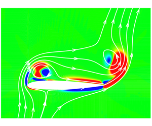
Figure 5. Contours of the vortex moment coefficient per unit area (left) and the vorticity (right) at typical instants: (a)  $\unicode[STIX]{x1D70F}=0.5$, (b)
  $\unicode[STIX]{x1D70F}=1.0$, (c)
  $\unicode[STIX]{x1D70F}=2.0$, (d)
  $\unicode[STIX]{x1D70F}=3.5$, with streamlines drawn.
4.3 Moment contribution related to the vortex evolution
To illustrate how a quantitative understanding of the moment contribution and the evolution of the vortical field can be gained from a VMM, the moment distribution about the quarter chord is plotted in figure 5(left-hand column) for three typical instants ( $\unicode[STIX]{x1D70F}=0.5,1,2$ and
  $3.5$) in the first period of the starting flow of the NACA0012 airfoil at
  $\unicode[STIX]{x1D6FC}=60^{\circ }$ and
  $Re=1000$, together with contour plots of the vorticity (right-hand column). The streamlines are also shown in this figure. The vorticity contours apparently show that the vorticity is concentrated in the boundary layer vortex sheet as well as the LEVs and TEVs being shed from the body. The boundary layer vortex sheet in the rear part of the airfoil (
 $x/c>1/4$) contributes significantly to the body moment, which can be attributed to the suction effect of the vortex sheet producing a positive (nose-down) pitching moment on the upper surface and a negative (nose-up) moment on the lower surface. For most snapshot instants, these positive and negative moments offset each other. It is clear that both LEVs and TEVs consist of a positive moment contributing area (red) and a negative one (blue). As the LEV grows and convects away from the body surface, the positive area reduces and the negative area increases, resulting in a reduction on the net moment contribution. This is likely due to the concentrated LEV (with a negative strength) moving away from the LE, which has been shown to contribute a nose-up moment in figure 1. Conversely, the TEV always contributes a net nose-down moment and it can be seen that the positive contributing area is always far more significant than the negative area.
It can thus be concluded that, in the case of starting flow on a NACA0012 airfoil presented here, the increase of the moment is determined by the roll up of the TEV, whereas the decrease is caused by the LEV and TEV moving away from the body.
5 Conclusion
The VMM method for viscous flow around an arbitrary two-dimensional body has been generalized. The proposed VMM approach expresses the vortex moment as a function of the vector product of a VMM vector and the local velocity. The VMM vector can be easily obtained by solving a Laplace equation by a vortex panel method. The VMM vector, a function of the position, is independent of the flow and only dependent on the geometry of the body. Thus a VMM can be designed and precomputed to help analyse the moment contribution effect of each given vortex and, extract the moment from a flow field given by CFD or experimental data.
VMM analysis based on NACA0012 airfoil shows that a LEV moving away from the reference point or a TEV moving towards the reference point contributes to a nose-down pitching moment, and vice versa. Moreover, for any reference points located on the airfoil except for the LE and TE, a LEV moving away from the edges or a TEV moving towards the edges contributes to a nose-up pitching moment, and vice versa.
The proposed VMM method is insensitive to vortices far away from the body, and reflects the fact that pressure loads on the airfoil are mainly due to near-body vortices, in accordance with the Biot–Savart law. As a test case, the precomputed VMM, together with the vortices obtained by CFD, has been used to predict the vortex moment on an impulsively started NACA0012 airfoil. The moments given by CFD itself are used as validations. The time-averaged moments about the quarter chord of the airfoil for a range of AoAs have been compared with experimental results given by Ohtake et al. (Reference Ohtake, Nakae and Motohashi2007) and Rainbird (Reference Rainbird2016). CFD has shown, as expected, that the contribution from viscous forces to the pitching moment is negligible for a large range of Reynolds numbers ( $Re\geqslant 50$), which means the compact vortex moment expression derived here for inviscid flows is eligible to deal with viscous flow problems and the corresponding VMM can accurately reflect the total force contribution of the vortices in the viscous flow field. It has been found that the unsteady nose-down moment about the quarter chord is higher than the steady-state value. The increment is mainly contributed by the roll up of LEVs and TEVs. By identifying the moment contributions from LEVs and TEVs in starting flows around a NACA0012 airfoil, we have shown that a moment map could lead to an intuitive understanding of how each part of the vorticity field contributes to the pitching moment on the body. It has been found that both LEVs and TEVs consist of a positive moment contributing area and a negative one. As a LEV grows and moves away from the body, its net contribution of moment changes from positive to negative, while a TEV always contributes a net positive moment. The time variation of the total moment is the overall effect of both LEVs and TEVs.
Acknowledgements
This project has received funding from the European Union’s Horizon 2020 research and innovation programme under the Marie Sklodowska-Curie grant agreement no. 765579.
Declaration of interests
The authors report no conflict of interest.


