


1. INTRODUCTION
Due to their flexibility and autonomy, AUVs (autonomous underwater vehicles) are used to explore underwater environments (Burlutskiy et al., Reference Burlutskiy, Touahmi and Lee2012; Allotta et al., Reference Allotta, Caiti, Costanzi, Fanelli, Fenucci, Meli and Ridolfi2016; Cao et al., Reference Cao, Zhu and Yang2016; Yu et al., Reference Yu, Xiang, Lapierre and Zhang2018; Zhang et al., Reference Zhang, Zhang, Chemori and Xiang2018; Gan et al., Reference Gan, Zhu, Hu, Yang, Shi and Chen2019) and for scientific investigation. As a development of information technology, sensors are used to monitor conditions of the oceans. Due to limited communication distance, the data stored in these sensors are mostly collected by tools such as multi-AUV systems. Multi-AUV systems are attracting much attention in this field. Task allocation within the multi-AUV system has become a hot topic in recent years (Chang et al., Reference Chang, Bian, Yan and Wang2004; Li et al., Reference Li, Zhang and Yang2014; Zhu et al., Reference Zhu, Qu and Yang2019).
The following methods are widely used in task allocation. Conventional task allocation strategies include market mechanisms (Akkiraju et al., Reference Akkiraju, Keskinocak, Murthy and Wu2001; Sariel et al., Reference Sariel, Balch and Stack2006; Sotzing and Lane, Reference Sotzing and Lane2010; Wang and Feng, Reference Wang and Feng2011), contract net algorithm and distributed world model. In a market-based system, the multi-robot system is considered as an economy and each robot is considered as an agent. The algorithm has been applied to task assignment for AUVs, but the algorithm cannot guarantee the optimisation of task assignment when the destination quantity is unknown. The contract net algorithm has been used for task allocation in a multi-AUV system, and the method was used to solve the problem in an heterogeneous multi-AUV system (Li and Zhang, Reference Li and Zhang2017). The distributed world model was presented to solve the problem of a cooperative robotic team under communication constraints (Tsiogkas et al., Reference Tsiogkas, Papadimitriou, Saigol and Lane2014). However, these methods cannot solve the problem of task allocation when the number of targets is unknown. Due to the similarity between the self-organising map (SOM) algorithm and task allocation, the SOM has been applied to task allocation (Tambouratzis, Reference Tambouratzis2006; Muslim et al., Reference Muslim, Ishikawa and Furukawa2007; Huang et al., Reference Huang, Zhu and Yuan2012; Wang et al., Reference Wang, Chen and Hung2015; Liu and Zhu, Reference Liu and Zhu2017; Zhu et al., Reference Zhu, Liu and Sun2017). The SOM neural network was first proposed by Kohonen in the 1980s (Kohonen et al., Reference Kohonen, Kaski, Lagus, Salojarvi, Honkela, Paatero and Saarela2000). The method is used for dynamic classification of input vectors. Targets are allocated to the corresponding robot according to the Euclidean distance. The SOM algorithm (Zhu et al., Reference Zhu, Huang and Yang2012) effectively solves the problem of an unknown number of targets. With the development of sensor technology, a strategy is needed to solve the problems that arise when using a limited number of AUVs to complete tasks, such as data collection from sensors.
The traditional SOM algorithm has two limitations in task allocation and path planning. First, the method relies on the order of the input vector. Because the number of AUVs is less than the number of targets, there exists a problem with accessible order of the targets for the AUV. When the order of the input vector is changed, the method may cause the large energy consumption mainly because AUV has reentrant path. Second, the performance of the total task assignment is bad. Because a single AUV carries limited energy, each AUV may not be assigned too many tasks, although the AUV is the nearest to the target. At the same time, the target is assigned to the farther AUV. Hence, the traditional algorithm may cause greater energy consumption overall. The traditional SOM algorithm cannot give the accessible order of targets for AUVs in a case where the number of targets is much greater than that of AUVs.
The classified SOM algorithm is presented to solve this problem. A single AUV is matched with a corresponding group of targets, and the classified SOM method then calculates the navigation distance between the AUV and each target in the group. The target with the minimum navigation distance is the first accessible target of the AUV. The location of the AUV is then updated to the location of that target until all the targets in the group have been accessed by the AUV. This method can give a more efficient accessible order of targets for AUVs and it enables the AUVs to visit targets while guaranteeing the least total energy consumption. AUVs may have different kinematics and dynamics from unmanned aerial vehicles (UAVs), but the task allocation problems for them share certain similarities. The improved algorithm may be used in more fields where the task allocation problems share certain similarities, such as UAVs (Sujit and Beard, Reference Sujit and Beard2007; Xiang et al., Reference Xiang, Liu, Su and Zhang2017).
The structure of the paper is as follows. A description of the task allocation problem is presented in Section 2. In Section 3, the classified SOM algorithm is proposed to solve the issue. In order to prove the effectiveness of the proposed method, the simulation and its results are given in Section 4. In Section 5, the conclusion is presented.
2. DESCRIPTION OF TASK ALLOCATION PROBLEM
In task allocation, tasks (target sensors) are effectively allocated to agents (AUVs) through a certain strategy. The task allocation problem is thus an assorted optimisation issue. Path planning is how to select the reasonable path and accessible order (in this case) for an AUV to access target sensors. The task allocation problem is illustrated in Figure 1, with eight targets (green dots) and three AUVs (pink dots) in the workspace. We evaluate the AUV consumption by the navigated distance from its starting position to its destination. The main issue of the multi-AUV system is how to divide the whole task into several subtasks so that AUVs can move to their designated targets along optimized paths.
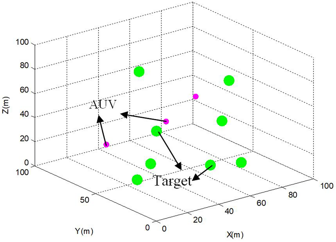
Figure 1. AUVs and targets randomly distributed.
3. ALGORITHM ANALYSIS
3.1. Traditional SOM task allocation algorithm
SOM is a clustering and unsupervised learning algorithm for high dimensional visualisation. It is very similar to the task assignment problem, so the SOM algorithm can be used to solve the issue of task assignment. The structure of SOM is shown in Figure 2. The SOM neural network is a network consisting of two layers. The input layer is the location coordinate of the target. The output layer is the location coordinate of the AUV, and each neuron in the output layer connects through the weight vector to neurons in the input layer. According to the SOM algorithm, the task allocation problem is divided into several sub-problems including the selection of the winning neuron, the definition of the neighbourhood function and the update of the weight vector.

Figure 2. Structure of the SOM algorithm.
First, the weight vector is used to select the winning neuron, and the neighbour neurons are decided by the neighbourhood function. Then, the winner and neighbour neurons move to the target. When (in this case) the target has been accessed by an AUV, that AUV becomes free for re-assignment. When all the targets have been accessed, the task allocation and path planning are completed.
3.1.1. Winner
The selection of the winner is defined as follows (Zhu et al., Reference Zhu, Huang and Yang2012):
 $$[P_j]\Leftarrow {\rm min}\{ D_{kjl},k = 1,2, \ldots ,K;j = 1,2, \ldots J;l = 1,2, \ldots ,L\} $$
 where  $[ {P_{j} } ]$ represents that the jth neuron from the kth group is the selected winner to the lth input node. D kjl is a value related to the Euclidean distance between the AUV and the target. The selection of the winner depends on the definition of the D kjl. The Euclidean distance is expressed as:
 $$|T_l-R_{jk}| = \sqrt {{(x_l-w_{jkx})}^2 + {(y_l-w_{jky})}^2 + {(z_l-w_{jkz})}^2} $$
 $T_{l} =( {x_{l} , \; y_{l} , \; z_{l} } ) , \; $ which is the lth target's coordinate, is the location of the lth target in the three-dimensional workspace.
  $R_{jk} =( {w_{jkx} , \; w_{jky} , \; w_{jkz} } ) $, which is the coordinate of the AUV in real time, is the location of the jth neuron from the kth group. Due to the limited energy available, the parameter P is used to adjust the energy consumption of the AUV. P is defined as:
 $$W=\frac{P_j - \bar{W}}{S+ \bar{W}}$$
S is the safe distance, where the navigational energy consumption of an AUV is less than the amount of energy it carries.  $\bar{W}$ is the average moving length of a team of AUVs in a certain task. Pj is the actual navigation length of the AUV. D kjl is defined as:
 $$\label{eq4} D_{kjl} =\left\{ {{\begin{array}{@{}l@{\quad}l@{}} {\vert {T_l -R_{jk} } \vert } & {\mbox{ 0}\le P_j \le S} \\ {\vert {T_l -R_{jk} } \vert \mbox{ }(1+W)} & {\mbox{S}\le P_j \le S_{\max} } \\ \infty & {\mbox{ }P_j \ge S_{\max } } \\ \end{array} }} \right.$$
 Here, the maximal length of a single AUV navigational is represented by S max. There are three different cases in Equation (4). First, 0 ≤ P j ≤ S, where the actually navigation distance is less than the safe distance, does not need  $\overline W $ to adjust the energy consumption. Second,
  $\overline W $ is used to adjust the energy consumption in a case where the actual navigation distance is greater than the safe distance. Finally, when the actual navigation distance is greater than the maximum navigation length, an AUV cannot be assigned to the target.
3.1.2. Neighbourhood function
The weights of winner and neighbour neurons are dependent on the neighbourhood function. The neighbour neurons are calculated as follows:
 $$\label{eq5} f(d_m ,g)=\left\{\begin{array}{@{}l@{\quad}l@{}} {e^{-{d_m^2 } / {g^2(t)}},} & {d_m < \lambda } \\ {0,\mbox{ }} & {\mbox{others}} \\ \end{array}\right.$$
 Radius λ represents the neighbour scope where the centre is the winning neuron.  $d_{m} =\vert {N_{m} -N_{j} } \vert $ denotes the distance between the m th AUV and the winning neuron. The function g 2(t) is defined as follows:
 $$\label{eq6} g^2(t)=(1-\partial )^tg_o$$
∂ is a fixed learning rate and ∂ < 1. The calculation time is decreased as the ∂ increases. The update rule is defined as:
 $$\label{eq7} R_{jk} (t+1)=\left\{\begin{array}{@{}l@{\quad}l@{}} {T_l ,} & {D_{kjl} \le D_{\min } } \\ {R_{jk} (t)+\partial \times f(d_m ,g)\times (T_l -R_{jk} (t)),} & {D_{kjl} >D_{\min } } \\ \end{array}\right.$$
In one case, where D min, which represents the termination condition of iterations, is greater than D kjl, the weight is replaced by the target coordinate. In another case, the weight's adjustment depends on the learning speed ∂, neighbourhood function f(d m, g) and the location of the winner and neighbours.
A flow chart of the SOM algorithm is presented in Figure 3. First, it initialises the location coordinates of the AUV and targets. Second, the location coordinates of the targets are input into the input layer and the location coordinates of the AUV are input into the output layer. According to the Euclidean distance, the winning neuron is selected through competition. Then the method calculates the neighbourhood function and adjusts the weight vectors. If the weight vectors change, the AUV moves towards the target point. When the weight vectors do not change, the task assignment and path planning are complete.
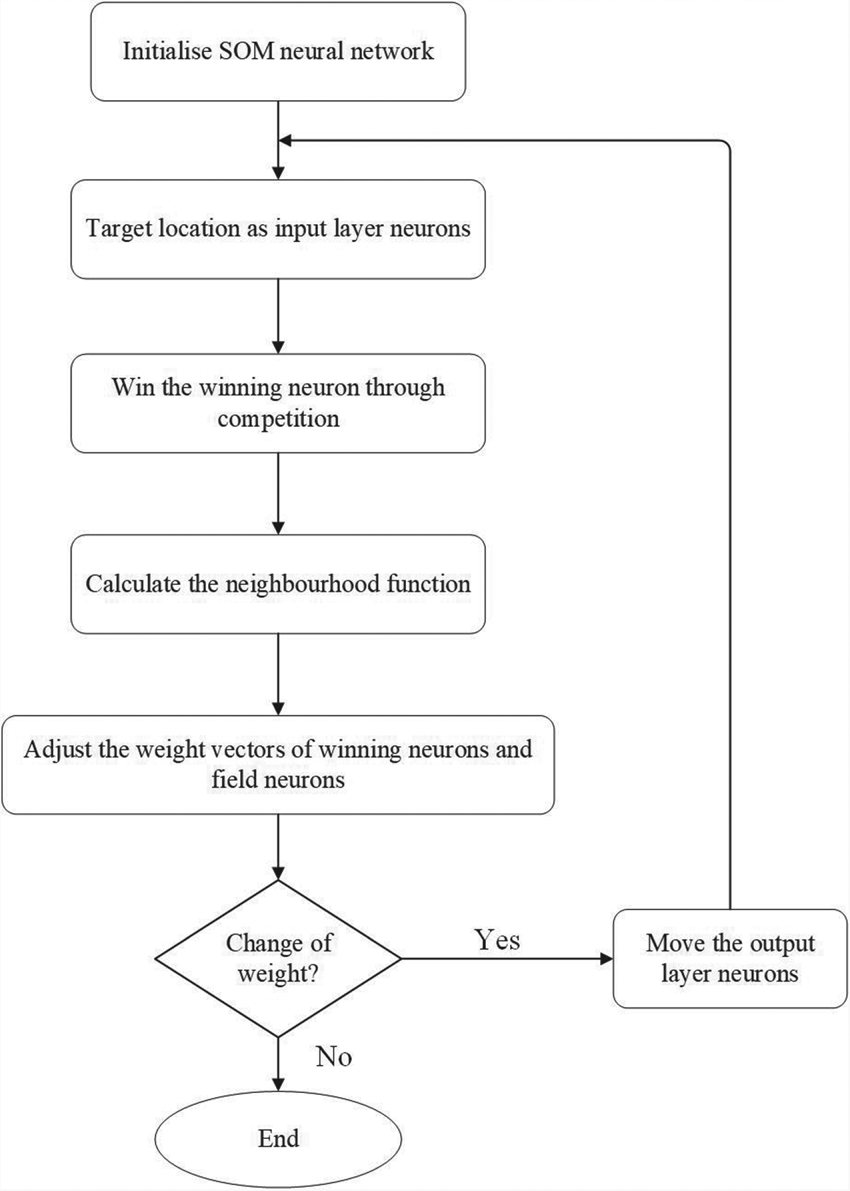
Figure 3. Flow chart of the SOM algorithm.
The traditional SOM method has two limitations in task allocation and path planning, as explained above, in its inability to solve the problem of accessible order of targets for the AUV and to take energy consumption into account.
3.2. Classified SOM algorithm
In order to solve the problem of accessible order of targets for the AUVs and to minimise the total energy consumption of the AUV system, the classified SOM (CSOM) algorithm is proposed. An algorithm flow chart of the CSOM method is presented in Figure 4. First, the location coordinates of AUVs and targets are initialised. According to the K-means algorithm, targets are classified into groups which are determined by the number of AUVs. The centres of groups are then matched with AUVs. The SOM algorithm is then used for task allocation and path planning.

Figure 4. Flow chart of the CSOM algorithm.
3.2.1. Classify the targets
The K-means algorithm is used to classify the targets. The number of groups depends on the number of AUVs. The flow chart of this method is shown in Figure 5. First, the location coordinates of centres and targets are initialised. D kn, which denotes the distance between centres and targets, is defined as:
 $$D_{kn} = \sqrt {{(C_k-T_n)}^2} $$
C k represents the kth centre and the number of centres depends on the number of AUVs, as shown in Figure 6. T n represents the coordinate location of the nth target. S kn is defined as:
 $$S_{kn}\Leftarrow \min \{ D_{kn},k = 1,2, \ldots ,K;n = 1,2, \ldots ,N\} $$
S kn belongs to the kth group, because the nth target is the nearest to the kth centre. Then, according to the location of targets in the group, the method calculates the centre of each group. When the centres are fixed, the grouping is completed. C k represents the kth centre of group. An example is shown in Figure 6, where pink dots represent five AUVs and green dots represent 20 targets. In this example, based on the number of AUVs, the targets are classified into five groups.

Figure 5. Flow chart of K-means.

Figure 6. Classification of targets.
3.2.2. AUVs matched with groups
When the targets have been classified into several groups, the centres of the groups are matched with AUVs. M ki is defined as:
 $$M_{ki} = \sqrt {{(C_k-R_i)}^2} $$
where M ki represents the Euclidean distance between the kth centre and the ith robot (AUV). CR ki represents the ith robot which is the nearest to the kth centre and is defined as:
 $$CR_{ki}\Leftarrow \min \{ M_{ki},k = 1,2, \ldots ,K\} $$
An example is shown in Figure 7, where again the pink dots represent five AUVs and green dots represent 20 targets. C k represents the kth centre of group. According to the Euclidean distance between AUVs and centres, AUVs are matched with the centres of the several groups.

Figure 7. AUVs matched with the groups of targets.
3.2.3. Improved SOM method in task allocation
After the AUVs have been matched with groups, the improved SOM method is used to allocate tasks to the AUV in each group. The improved SOM method changes the connected relation between the AUV and targets. The structure of the improved SOM method is presented in Figure 8. The input layer neuron is dynamic. A single AUV connects with all targets. The AUV is allocated to the targets in the group according to the shortest actual navigation distance to each. The target that represents the minimum navigation distance in the group is the first accessible target of the AUV. When an AUV accesses a target, the location of the AUV is updated to the location of that target until all targets in the group have been accessed by the AUV. As shown in Figure 9, the pink dot represents the AUV and the green dot represents the target. α represents the angle between the x-axis and the black dotted line that connects the AUV and the target point at the initial time. θ is the initial orientation of the AUV and r is the turning radius of the AUV. β is defined as follows:
 $$\beta = \theta -\alpha $$
 The AUV has two turning paths, shown as the red solid line and the red dotted line in Figure 9. The AUV is steered in the direction of  $\vert \beta \vert $ at decreasing distance until β = 0. The actual path travelled by the AUV is the red solid line plus black line in Figure 9. D uj is defined as:
 $$D_{uj} = \Delta U + |R_u-T_j|$$
 where D uj represents the actual navigation distance. Δ U is the turning distance of the uth AUV when turning to β = 0.  $\vert {R_{u} -T_{j} } \vert $ is the Euclidean distance between the jth target and the uth turning AUV. The accessible order of targets to the AUV depends on the [Ai]. The selection of the nearest target is defined as
 $$[Ai]\Leftarrow \min \{ D_{uj}{\rm , }j = 1,2, \ldots J\} {\rm }$$
where [Ai] represents the nearest target to the uth AUV. J is the number of targets in the corresponding group. The method then calculates the neighbourhood function and adjusts the weight vectors. If the weight vectors are changed, the AUV moves towards the target point. When the location of the AUV is updated to the location of the target, the AUV becomes free and the remaining targets are input into the input layer. When all targets have been accessed by the AUV, the task allocation and path planning are completed for that group.

Figure 8. Structure of the improved SOM algorithm.
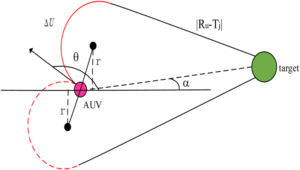
Figure 9. Actual navigation distance of AUV.
4. SIMULATION
Due to random errors in the position, speed, angle and turning radius of AUVs, the error datum are processed with extended Kalman filter (Loebis et al., Reference Loebis, Sutton, Chudley and Naeem2004; Wu et al., Reference Wu, Ta, Xiao, Wei, An and Li2019). For example, in Figure 10, the black line represents the actual value of the AUV, the blue line represents the measured value and the red line represents the extended Kalman filter estimated value. To increase the accuracy of the error datum, all datum are processed with the extended Kalman filter.

Figure 10. Extended Kalman filter algorithm.
4.1. Two-dimensional plane simulation results
The study of the three-dimensional algorithm is based on the study of the two-dimensional algorithm. The simulation results of the two-dimensional algorithm reflect the effectiveness more intuitively. The location coordinates of AUVs are set to random number seed 5. The location coordinates of targets are set to random number seed 15. The turning radius of the AUV is 0·8 and its running speed is 1·5 m/s. For R1, the angle between R1 and the x-axis is θ1 and θ1 is 150°. The angles of R2 and so on are shown in Figures 11 and 12. The traditional SOM is presented in Figure 11. There are 25 targets (green dots) and five AUVs (R1 … R5) (pink dots) in the workspace. Due to the problem of the input order in the traditional method, when the target is input in the input layer, the winner (AUV), which is the nearest to the target, is selected for the target. Although the target is allocated to the nearest AUV, another target, which is not allocated, is nearer to the AUV. This can cause more energy consumption for the AUV. For example, R1 is nearest to T1, but R1 accesses T3 first. The accessible order of targets for R1 clearly causes more energy consumption. The total distance travelled by the AUVs (as a proxy for energy consumption) is 725·6460 m in the traditional method.
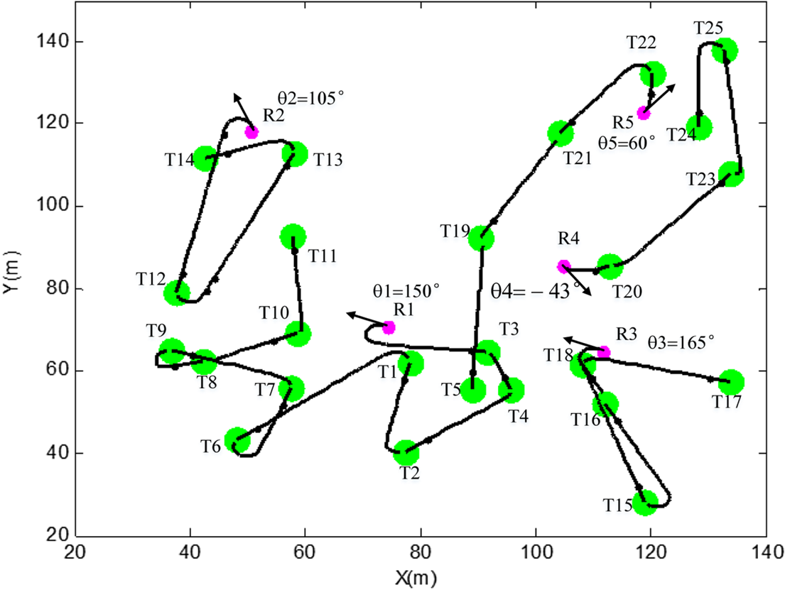
Figure 11. The traditional SOM method.

Figure 12. The CSOM method.
In Figure 12, the location coordinates of the five AUVs (pink dots) and targets are the same as in Figure 11. Based on the number of AUVs, the targets are now divided into five groups. The green dots are allocated to R1, the blue dots are allocated to the R2, the black dots are allocated to the R3, the yellow dots are allocated to the R4, and the red dots are allocated to the R5. For example, T11, T13 and T14 are allocated to R2. According to the actual navigation distance between the AUV and the target, the CSOM method can give the most efficient accessible order of targets for the AUV. The total distance travelled by the AUVs is 599·9616 m in the CSOM method. The accessible order of targets to the AUVs is more efficient in the CSOM than the traditional SOM, and the CSOM method can also save energy consumption by reducing the distance travelled by the AUVs.
Figures 13 and 14 illustrate the effects on energy consumption in terms of distance travelled. In Figure 13 the x-axis represents the number of targets and the y-axis represents the total energy consumption of the AUVs. The red line represents the total energy consumption of the CSOM method and the black line represents that of the SOM method. There is an intersection of the two lines and the abscissa of the intersection is seven. When the number of targets is more than seven, the total energy consumption in the CSOM is less than in the traditional SOM. When the number of targets is less than seven, the total energy consumption in the traditional SOM is less than in the CSOM. Because there are three AUVs in the workspace, there is no need to classify targets because the number of AUVs is close to the number of targets. As the number of targets increases, the energy consumption gap between the CSOM method and the traditional SOM method increases. In Figure 14, the x-axis represents the number of AUVs and the y-axis represents the total energy consumption. The red line represents the total energy consumption of the CSOM method and the black line represents that of the traditional SOM method. There are 40 targets and some AUVs in the workspace environment. In Figure 14, as the number of AUVs increases, the total energy consumption in the CSOM is less than the SOM.

Figure 13. Total energy consumption of AUVs by number of targets (Tnum = 0–45).

Figure 14. Total energy consumption of AUVs by number of AUVs (Rnum = 5–10).
The CSOM method can save energy in the case where the number of targets is much greater than the number of AUVs, and it can also give a more efficient accessible order of targets than in the traditional SOM method.
4.2. Three-dimensional plane simulation results
The location coordinates of AUVs are set to random number seed 8. The location coordinates of targets are set to random number seed 4. The turning radius of the AUV is 0·8 and its running speed is 1·5. The initial angles of the AUVs (R1–R3) are illustrated in Table 1. The traditional SOM is presented in Figure 15. There are 12 targets (green dots) and three AUVs (pink dots) in the workspace. With SOM, the same problem exists in the three-dimensional plane as in the two-dimensional plane. For example, R3 is nearest to T11, but it accesses T10 first, which clearly causes more energy consumption. The total distance travelled by the AUVs is 631·0219 m in the traditional SOM method. In Figure 16, the location coordinates of AUVs and targets are the same as in Figure 15. The pink dots represent AUVs and the other coloured dots represent targets. Based on the number of AUVs, the targets are now divided into three groups. The blue target dots are allocated to R1, the green target dots are allocated to R2, and the red target dots are allocated to R3. For example, T11, T12 and T9 are allocated to R3. The total distance travelled by the AUVs is 440.3366 m in the CSOM method.
Table 1. Initial orientation of the robot (AUV) in three-dimensional plane.


Figure 15. The traditional SOM method in three-dimensional plane.

Figure 16. The CSOM method in three-dimensional plane.
4.3. Large number simulation results
Further simulations were conducted with larger numbers of AUVs and targets to justify the methodology proposed. Figures 17 and 18 illustrate the energy consumption. Figure 19 models the CSOM method where the number of targets (40) greatly exceeds number of AUVs (5) in two and three dimensions. In Figure 17 the x-axis represents the number of targets (0–70) and the y-axis represents the total energy consumption of the AUVs in terms of distance travelled. The red line represents the total energy consumption of the CSOM method and the black line represents that of the SOM method. There is an intersection of the two lines and the abscissa of the intersection is 10. When the number of targets is more than 10, the total energy consumption in the CSOM is less than that in the SOM. When the number of targets is less than 10, the total energy consumption in the SOM is less than that in the CSOM. If there were five AUVs and 10 targets in the workspace, it would not be necessary to classify the targets because the number of AUVs would be close to the number of targets. As the number of targets increases, the energy consumption gap between the CSOM method and the SOM method increases. In Figure 18, the x-axis represents the number of AUVs (2–14) and the y-axis represents the total energy consumption in terms of distance travelled. The red line represents the total energy consumption of the CSOM method and the black line represents the total energy consumption of the SOM method. There are 40 targets and some AUVs in the workspace environment. In Figure 18, as the number of AUVs increases, the total energy consumption in the CSOM becomes less than that in the SOM.

Figure 17. Total energy consumption of AUVs by number of targets (Tnum = 0–70).

Figure 18. Total energy consumption of AUVs by number of AUVs (Rnum = 2–14).
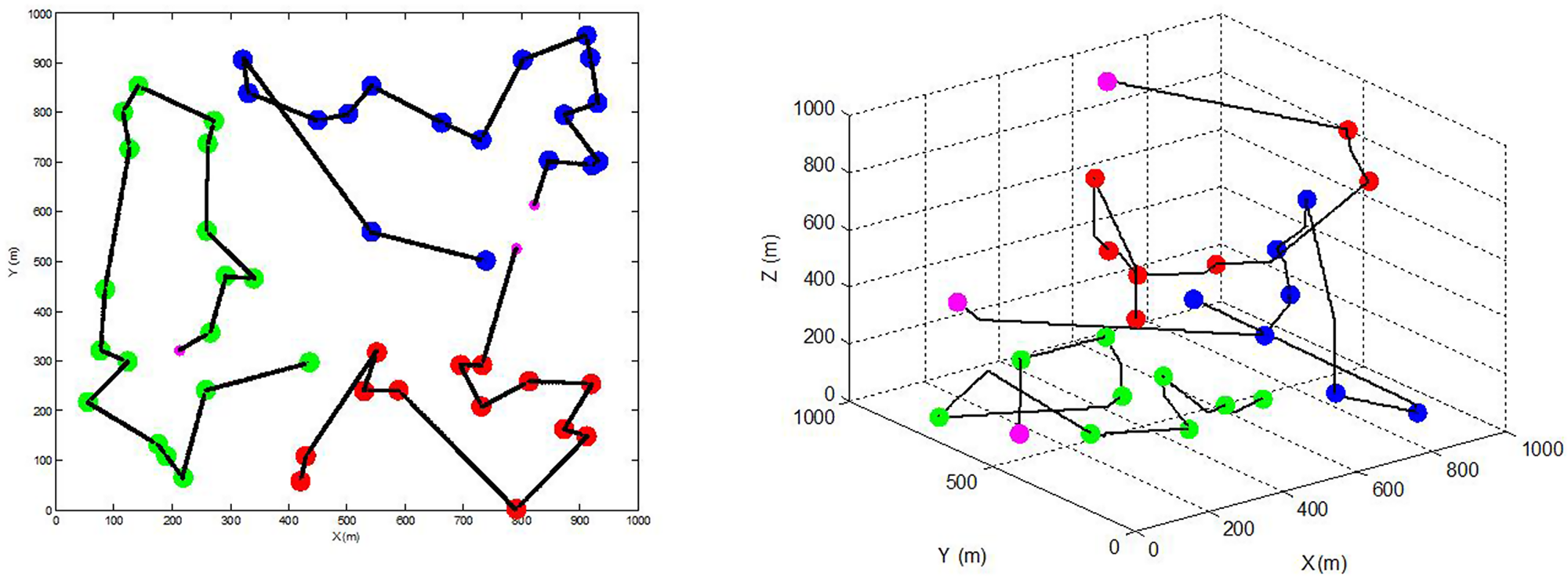
Figure 19. CSOM method where number of targets greatly exceeds number of AUVs: two-dimensional plane (left) and three-dimensional plane (right).
The concrete analyses are the same as in Figures 12 and 16. As the gap between the number of AUVs and the number of targets increases, the different levels of energy consumption are illustrated in Figures 13, 14, 17 and 18.
5. CONCLUSION
In this paper, a classified SOM algorithm is proposed. The CSOM algorithm not only gives a more efficient accessible order of targets for the AUVs than the SOM method, but it can also reduce energy consumption. Given that each AUV carries a limited supply of energy for each mission, the CSOM method can enable AUVs to access more targets than the SOM method in the same environment. Future research will explore the effect of ocean currents on the task assignment problem for AUV systems. An ocean current is described by its velocity and direction in the actual underwater environment. By measuring the ocean current in a certain period of time, the ocean current average is obtained. The ocean current average is used as the constant ocean current for modelling the underwater working environment. The CSOM method can thus be extended to the ocean environment. It can also be extended to cases where targets have different priorities.
ACKNOWLEDGEMENTS
This project is supported by the National Natural Science Foundation of China (U1706224, 51575336, 91748117) and the Creative Activity Plan for Science and Technology Commission of Shanghai (18DZ2253100, 18JC1413000, 18DZ1206305)


