2 Notations and the statement of main results

For reader’s convenience, we recall some basic Sobolev spaces which are standard in dealing with elliptic and parabolic partial differential equations.

Let $\alpha\in (0,1)$ . We denote by $C^{\alpha, \frac{\alpha}{2}}(\bar{Q}_{T})$ the Hölder space in which every function is Hölder continuous with respect to (x,t) with exponent $(\alpha,\frac{\alpha}{2})$ in $\bar{Q}_{T}$ .

Let $p>1$ and V be a Banach space with norm $||\cdot||_v$ , we denote

\[ L^p(0,T; V)=\{ F(t): t\in [0,T]\rightarrow V: ||F||_{L^p(0,T;V)}<\infty\},\]

equipped with norm

\[ ||F||_{L^{p}(0,T;V)}=\left(\int_{0}^{T} ||F||_v^p dt\right)^{\frac{1}{p}}.\]

When $V=L^{p}(\Omega)$ , we simply use

\[ L^p(Q_{T})=L^{p}(0,T;L^{p}(\Omega)).\]

Moreover, the $L^p(Q_{T})$ -norm is denoted by $||\cdot||_p$ and $||\cdot||_{\infty}$ when $p=\infty$ for simplicity.

Sobolev spaces $W_{p}^{k}(\Omega)$ and $W_{p}^{k,\,l}(Q_{T})$ are defined the same as in the classical books such as [Reference Evans10] and [Reference Ladyzenskaja, Solonikov and Uralceva16].

Let $V_2(Q_T)=\{ u(x,t)\in C([0,T];W_{2}^{1}(\Omega)): ||u||_{V_{2}}<\infty\} $ equipped with the norm

\[ ||u||_{V_{2}}=\sup_{0\leq t\leq T}||u||_{L^{2}(\Omega)}+\sum_{i=1}^{n}||u_{x_{i}}||_{2}.\]

For any $\mu\in [0, n+2)$ , the Morrey–John–Nirenberg–Campanato space $L^{2, \mu}(Q_{T})$ is defined as in [Reference Campanato6]. Particularly, when $\mu=0$ ,

\[ L^{2,0}(Q_{T})=L^2(Q_{T}),\]

and when $\mu\in (n, n+2)$ , $L^{2, \mu}(Q_{T})$ is equivalent to the classical Hölder space $C^{\alpha, \frac{\alpha}{2}}(\bar{Q}_{T})$ with

\[ \alpha= \frac{(n+2)-\mu}{2}.\]

We first state the basic assumptions for the diffusion coefficients and known data. All other parameters in equations (1.1)–(1.4) are assumed to be positive automatically throughout this paper. We also choose $h(s)=\frac{s}{s+K}$ for simplicity.

H(2.1). Assume that $d_i(x,t)\in L^{\infty}(\Omega\times (0,\infty))$ for all i. There exist two positive constants $d_0$ and $D_0$ such that

\[ 0<d_0\leq d_i(x,t)\leq D_0,\quad (x,t)\in Q_{T}.\]

H(2.2). Assume that all initial data $S_0(x), I_0(x), R_0(x), B_0(x)$ are nonnegative on $\Omega$ . Moreover, $U_0(x)=(S_0(x),I_0(x),R_0(x),B_0(x))\in L^{2}(\Omega)^4.$

H(2.3). Let $0\leq b(x,t)\in L^{\infty}(Q)$ . Moreover,

\[ ||b||_{L^{\infty}(Q)}\leq b_0<\infty.\]

For brevity, we set

\[ u_1(x,t)=S(x,t), u_2(x,t)=I(x,t), u_3=R(x,t), u_4(x,t)=B(x,t), \, (x,t)\in Q. \]

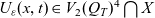
We use $U(x,t)=(u_1,u_2,u_3,u_4)$ to be a vector function defined in Q. The right-hand sides of the equations (1.1), (1.2), (1.3) and (1.4) are denoted by $f_1(U),\, f_2(U),\, f_3(U),\, f_4(U)$ , respectively. For convenience, we use $f_1(U)$ instead of $f_1(x,t,U)$ since $f_1$ depends on x,t and U. With the new notation, the system (1.1)–(1.6) can be written as the following reaction–diffusion system:

(2.1) \begin{eqnarray} & & u_{1t}-\nabla[d_1(x,t)\nabla u_1]=f_1(U),\quad (x,t)\in Q_{T},\end{eqnarray}

(2.2) \begin{eqnarray} & & u_{2t}-\nabla[d_2(x,t)\nabla u_2]=f_2(U),\quad (x,t)\in Q_{T}, \end{eqnarray}

(2.3) \begin{eqnarray}& & u_{3t}-\nabla[d_3(x,t)\nabla u_3]=f_3(U),\quad (x,t)\in Q_{T},\end{eqnarray}

(2.4) \begin{eqnarray} & & u_{4t}-\nabla[d_4(x,t)\nabla u_4]=f_4(U),\quad (x,t)\in Q_T, \end{eqnarray}

subject to the initial and boundary conditions:

(2.5) \begin{eqnarray} & & U(x,0)=U_0(x)=(S_0(x),I_0(x),R_0(x),B_0(x)),\quad x\in \Omega, \end{eqnarray}

(2.6) \begin{eqnarray} & & \nabla_{\nu}U(x,t)=0,\quad (x,t)\in \partial \Omega\times (0,T]. \end{eqnarray}

We define a product space X equipped with the standard product norm:

\[ X=L^{2}(0,T;W_{2}^{1}(\Omega))^{4}.\]

The conjugate dual space of X is denoted by $X^*$ .

Definition 2.1. We say U(x,t) is a weak solution to the problem (2.1)–(2.6) in $Q_{T}$ if $U(x,t)\in X$ such that

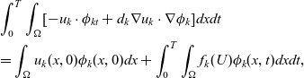\begin{eqnarray*} & & \int_{0}^{T}\int_{\Omega}[-u_k\cdot \phi_{kt}+d_k\nabla u_k\cdot \nabla\phi_k]dxdt\\ & & =\int_{\Omega} u_k(x,0)\phi_k(x,0)dx +\int_{0}^{T}\int_{\Omega} f_k(U)\phi _k(x,t)dxdt, \end{eqnarray*}

for any test function $\phi_k\in X^*\bigcap L^{\infty}(Q_{T})$ and $\phi_{kt}\in L^2(Q_{T})$ with $\phi_k(x,T)=0$ on $\Omega$ for all $k=1,2,3,4$ .

To obtain more regularity, we need additional regularity for known data.

H(2.4). Assume that $b(x,t)\in L^{2, \mu}(Q))$ for any $\mu\in [n, n+2)$ . Let $\nabla U_0(x)\in L^{2, \mu}(\Omega)^4$ for any $\mu\in [n-2, n)$ .

With some additional effort, we can prove that the solution is uniformly bounded in Q for any dimension n.

Theorem 2.3. Under the assumption H(2.1)–(2.4), the problem (2.1)–(2.6) has a unique global solution in $L^{\infty}(Q)\bigcap C^{\alpha, \frac{\alpha}{2}}(\bar{Q})$ . Moreover,

\[ ||U||_{L^{\infty}(Q)}\leq C,\]

where C depends only on known data.

With the result of Theorem 2.3, we can establish the global asymptotic behaviour of the solution.

H(2.5). Assume

\[\lim_{t\rightarrow \infty}b(x,t)=b_0(x), \lim_{t\rightarrow \infty}d_i(x,t)=d_{i\infty}(x),\qquad x\in \Omega, i=1, 2, 3, 4,\]

uniformly in $\bar{\Omega}$ . Moreover, $d_{i\infty}(x)\in C^{\alpha}(\bar{\Omega})$ for all i.

Let $S_{\infty}(x)$ be the steady-state solution for the following elliptic equation

(2.7) \begin{eqnarray} & & -\nabla[d_1(x)\nabla S_{\infty}]=b_0(x)-dS_{\infty},\qquad x\in \Omega \end{eqnarray}

(2.8) \begin{eqnarray} & & \nabla_{\nu}S_{\infty}(x)=0,\qquad x\in \partial \Omega. \end{eqnarray}

where $m_0=\max_{\bar{\Omega}}S_{\infty}(x)$ .

3 Global solvability and regularity

From the physical model, the concentration must be nonnegative. Here, we state this fact as a lemma and sketch a proof since we could not find precise reference in the literature. Recall that a vector function is said to be nonnegative if each component of the vector function is nonnegative.

Lemma 3.1: Assume the conditions H(2.1)–H(2.2) hold. Then, a weak solution U(x,t) of (2.1)–(2.6) must be nonnegative in Q:

\[ U(x,t)\geq 0, (x,t)\in Q_T.\]

Proof Recall that a vector function $F(x,t,U):=(f_1(x,t,U),f_2(x,t,U), \cdots, f_m(x,t,U))$ is said to be quasi-positive if for all $k=1, 2, \cdots, m$ ,

\[ f_k(x,t,u_1,u_2,\cdots, u_{k-1},0,u_{k+1}, \cdots, u_m)\geq 0, u_i\in [0, \infty), i=1, 2, \cdots, m, i\neq k.\]

Since $b(x,t)\geq 0$ , clearly, $F(x,t,U)=(f_1(U), \cdots, f_4(U))$ is quasi-positive. Moreover, $f_k(U)$ is locally Lipschitz continuous with respect to $u_k$ . For a function $v(x,t)\in L^2(Q_{T})$ , we define

\[ v^+(x,t)=\frac{|v(x,t)|+v(x,t)}{2}, v^-(x,t)=\frac{|v(x,t)|-v(x,t)}{2}.\]

Now, we consider a modified system (2.1)–(2.6) in which $f_i(U)$ is replaced by $f_i(U^+)$ . Then, we choose $\phi_k(x,t)=(T-t)u_{k}^{-}$ (one may need to use a truncation technique as in Lemma 1, p. 749, in [Reference Bendahmane, Langlais and Saad3], if necessary) to obtain, after some routine calculation,

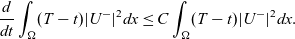\[ \frac{d}{dt}\int_{\Omega}(T-t)|U^-|^2dx\leq C\int_{\Omega}(T-t)|U^-|^2dx.\]

It follows that $u_{k}^{-}(x,t)=0$ in $Q_{T}$ , which implies that a weak solution to the modified system is the same as the original system (2.1)–(2.6).

As in the standard analysis in deriving an a priori estimate for solution of a partial differential equation, we may assume that the solution is smooth in $Q_{T}$ . A special attention is paid to be what a constant C depends precisely on known data in the derivation. We will denote by $C, C_1, C_2,\cdots,$ etc., generic constants in the derivation. Those constants may be different from one line to the next as long as their dependence is the same.

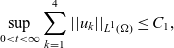
Lemma 3.2: Under the assumptions of H(2.1)–H(2.2), there exists a constants $C_1$ such that

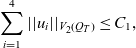\[ \sum_{i=1}^{4}||u_i||_{V_2(Q_{T})}\leq C_1,\]

where $C_1$ depends only on known data and the upper bound of T.

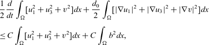
Proof From equations (2.1) and (2.3), we use the energy method to obtain

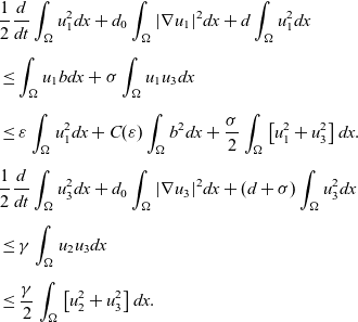\begin{align*}& \frac{1}{2}\frac{d}{dt}\int_{\Omega}u_1^2dx +d_0\int_{\Omega}|\nabla u_1|^2dx +d\int_{\Omega}u_1^2 dx\\[5pt] & \leq \int_{\Omega} u_1b dx +\sigma\int_{\Omega}u_1u_3 dx\\[5pt] & \leq \varepsilon \int_{\Omega}u_1^2dx +C(\varepsilon)\int_{\Omega}b^2dx +\frac{\sigma}{2}\int_{\Omega}\left[u_1^2+u_3^2\right] dx.\\[5pt] & \frac{1}{2}\frac{d}{dt}\int_{\Omega}u_3^2dx +d_0\int_{\Omega}|\nabla u_3|^2dx +(d+\sigma)\int_{\Omega}u_3^2dx\\[5pt] & \leq \gamma\int_{\Omega} u_2u_3 dx \\[5pt] & \leq \frac{\gamma}{2} \int_{\Omega}\left[u_2^2+u_3^2\right] dx.\end{align*}

It follows that

\begin{align*}& \frac{1}{2}\frac{d}{dt}\int_{\Omega}\left[u_1^2+u_3^2\right]dx +d_0\int_{\Omega}\left[|\nabla u_1|^2+|\nabla u_3|^2\right]dx\\[5pt] & +\left(d-\varepsilon-\frac{\sigma}{2}\right)\int_{\Omega}u_1^2dx +\left(d+\frac{\sigma}{2}-\frac{\gamma}{2}\right)\int_{\Omega}u_3^2dx\\[5pt] & \leq C(\varepsilon)\int_{\Omega}b^2dx +\frac{\gamma}{2}\int_{\Omega}u_2^2 dx.\end{align*}

To estimate $u_2$ , we must use the special structure of the system (1.1)–(1.4).

Let

\[ v(x,t)=u_1(x,t)+u_2(x,t),\quad (x,t)\in Q.\]

Then, we see that v(x,t) satisfies

(3.1) \begin{eqnarray} & & v_t-\nabla[d_2\nabla v]+dv=\nabla [(d_1-d_2)\nabla u_1]+b(x,t)-\gamma u_2+\sigma u_3,\quad (x,t)\in Q_{T}, \end{eqnarray}

(3.2) \begin{eqnarray}& & v(x,0)=S_0(x)+I_0(x), x\in \Omega; \,\nabla_{\nu}v=0, (x,t)\in \partial \Omega \times (0,\infty).\end{eqnarray}

The energy estimate for v from equations (3.1)–(3.2) yields

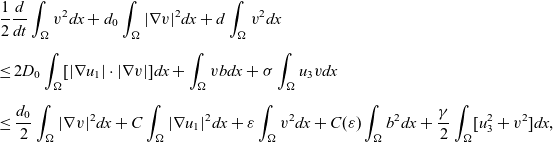\begin{eqnarray*}& & \frac{1}{2}\frac{d}{dt}\int_{\Omega}v^2dx +d_0\int_{\Omega}|\nabla v|^2dx +d\int_{\Omega}v^2dx \\[5pt] & & \leq 2D_0\int_{\Omega}[|\nabla u_1| \cdot |\nabla v|]dx+\int_{\Omega}vb dx +\sigma\int_{\Omega}u_3vdx\\[5pt] & & \leq \frac{d_0}{2}\int_{\Omega}|\nabla v|^2dx +C\int_{\Omega} |\nabla u_1|^2dx +\varepsilon \int_{\Omega}v^2dx +C(\varepsilon)\int_{\Omega}b^2dx +\frac{\gamma}{2}\int_{\Omega}[u_3^2+v^2]dx,\end{eqnarray*}

We combine the estimates for $u_1, u_3$ and v to obtain

\begin{eqnarray*}& & \frac{1}{2}\frac{d}{dt}\int_{\Omega}[u_1^2+u_3^2+v^2]dx+\frac{d_0}{2}\int_{\Omega}[|\nabla u_1|^2+|\nabla u_3|^2+|\nabla v|^2]dx\\[5pt] & & \leq C \int_{\Omega}[u_1^2+u_3^2+v^2] dx+C\int_{\Omega}b^2dx,\end{eqnarray*}

where C depends only on known data.

Gronwall’s inequality yields

\[ \int_{\Omega}[u_1^2+u_3^3+v^2]dx +\int_{0}^{t}\int_{\Omega}[|\nabla u_1|^2+|\nabla u_3|^2+|\nabla v|^2dx]dxdt\leq C+C\int_{0}^{T}\int_{\Omega}b^2dxdt,\]

where C depends only on known data and T.

It follows that

\[ ||u_1||_{V_{2}(Q_{T})}\leq C; \, ||u_3||_{V_2(Q_{T})}\leq C.\]

By the definition of v, we see

\[ ||u_2||_{V_{2}(Q_{T})}\leq C,\]

where C depends only on known data and the upper bound of T.

Once $u_2$ is bounded in $V_2(Q_T)$ , by equation (2.4), we easily obtain an estimate for $u_4$ :

\[||u_4||_{V_2(Q_{T})}\leq C,\]

where C depends only on known data.

With the estimates from the previous lemmas, we are now ready to prove Theorem 2.1.

Proof of Theorem 2.1 . There are several ways to prove the existence of a weak solution for the system (2.1)–(2.6). We use a truncation method. For any $\varepsilon>0$ , we denote by $\chi(u)$ the Heaviside function. Denote the smooth approximation of $\chi_{\varepsilon}(u)$ by

\begin{align*} \chi_{\varepsilon}(u)= \mbox{smooth approximation of $\chi\left(u-\frac{1}{\varepsilon}\right)$}.\end{align*}

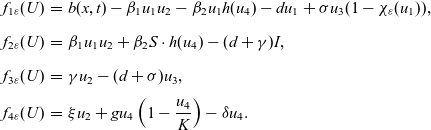\begin{eqnarray*}f_{1\varepsilon}(U) & = & b(x,t)-\beta_1u_{1}u_{2}-\beta_2 u_1h(u_4)-du_1+\sigma u_3(1-\chi_{\varepsilon}(u_1)),\\[5pt] f_{2\varepsilon}(U) & = & \beta_1u_1u_2+\beta_2S \cdot h(u_4)-(d+\gamma)I,\\[5pt] f_{3\varepsilon}(U) & = & \gamma u_2 -(d+\sigma)u_3,\\[5pt] f_{4\varepsilon}(U) & = & \xi u_2 +gu_4\left(1-\frac{u_4}{K}\right)-\delta u_4.\end{eqnarray*}

Now, we consider the following approximated reaction–diffusion system:

(3.3) \begin{eqnarray}& & u_{1 \varepsilon}-\nabla[d_1(x,t)\nabla u_1]=f_{1\varepsilon}(U),\qquad (x,t)\in Q_{T},\end{eqnarray}

(3.4) \begin{eqnarray} & & u_{2 t}-\nabla[d_2(x,t)\nabla u_{2}]=f_{2\varepsilon}(U), \qquad (x,t)\in Q_{T}, \end{eqnarray}

(3.5) \begin{eqnarray}& & u_{3 t}-\nabla[d_3(x,t)\nabla u_{3}]=f_{3\varepsilon}(U),\qquad (x,t)\in Q_{T},\end{eqnarray}

(3.6) \begin{eqnarray} & & u_{4 t}-\nabla[d_4(x,t)\nabla u_{4 }]=f_{4\varepsilon}(U),\qquad (x,t)\in Q_T, \end{eqnarray}

subject to the same initial and boundary conditions (2.5)–(2.6).

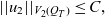
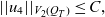
For the approximate problem (3.3)–(3.6) subject to initial-boundary conditions (2.5)–(2.6), by using the standard theory for parabolic equations (see [Reference Evans10] or [Reference Ladyzenskaja, Solonikov and Uralceva16]), we claim that there exists a unique weak solution in $V_2(Q_{T})\bigcap L^{\infty}(Q_{T})$ for every small $\varepsilon>0$ and

\[ \sum_{i=1}^{4}||u_{i\varepsilon}||_{L^{\infty}(Q_{T})}\leq C(\varepsilon),\]

where $C(\varepsilon)$ depends on known data and $\varepsilon$ .

For the completeness, we sketch a proof for the claim here. For the existence of a bounded weak solution $U_{\varepsilon}(x,t)$ , we use Leray–Schauder’s fixed-point theorem. Choose a Banach space $X=L^{\infty}(Q_{T})^4$ . For every $V(x,t)\in X$ and each $\lambda \in [0,1]$ , the standard theory of parabolic equations (see [Reference Ladyzenskaja, Solonikov and Uralceva16]) implies that there exists a unique weak solution $U_{\varepsilon}(x,t)\in V_2(Q_{T})^4\bigcap X$ for the following linear parabolic system:

\begin{eqnarray*}& & u_{1 \varepsilon}-\nabla[d_1(x,t)\nabla u_1]= \lambda f_{1\varepsilon}(V),\quad (x,t)\in Q_{T},\\[5pt] & & u_{2 t}-\nabla[d_2(x,t)\nabla u_{2}]= \lambda f_{2\varepsilon}(V),\quad (x,t)\in Q_{T}, \\[5pt] & & u_{3 t}-\nabla[d_3(x,t)\nabla u_{3}]=\lambda f_{3\varepsilon}(V),\quad (x,t) \in Q_{T},\\[5pt] & & u_{4 t}-\nabla[d_4(x,t)\nabla u_{4 }]= \lambda f_{4\varepsilon}(V),\quad (x,t)\in Q_T, \\[5pt] & & \partial_{\nu}U(x,t)=0, (x,t)\in \partial \Omega\times (0,T], U(x,0)=\lambda U_0(x), x\in \Omega. \end{eqnarray*}

We define a mapping $M_{\lambda}$ from X into X as follows:

\[ M_{\lambda}: V\in X \rightarrow U_{\varepsilon}=M_{\lambda}[V]\in X.\]

Clearly, the mapping $M_{\lambda}$ is well-defined and $M_0[V]=0$ . Moreover, DeGiorgi–Nash’s theory implies that all fixed-points of $M_{\lambda}$ satisfies

\[ ||U_{\varepsilon}||_{C^{\alpha, \frac{\alpha}{2}}(\bar{Q}_{T})}\leq C(\varepsilon),\]

where $\alpha\in (0,1)$ and $C(\varepsilon)$ is a constant which depends on $\varepsilon$ .

Since the embedding mapping from $C^{\alpha, \frac{\alpha}{2}}(\bar{Q}_{T})$ into $L^{\infty}(Q_{T})$ is compact, we can easily show that the mapping $M_{\lambda}$ is continuous and compact from X to $C^{\alpha, \frac{\alpha}{2}}(\bar{Q}_{T})$ . By Leray–Schauder’s fixed-point theorem, the problem (3.3)–(3.6) along with the initial-boundary conditions (2.5)–(2.6) has a weak solution $U_{\varepsilon}(x,t)\in V_2(Q_{T}\bigcap L^{\infty}(Q_{T})$ . Uniqueness follows from the fact that all weak solutions are bounded and $f_k$ is locally Lipschtz continuous with respect to $u_i$ .

Next, we see that all a priori energy estimates from Lemma 3.2 hold and these bounds are independent of $\varepsilon$ . Note that $U_{\varepsilon t}\in L^{2}(0,T;H^{-1}(\Omega))$ . By using the weak compactness of $L^{2}(Q_T)$ , we can extract a subsequence of $\varepsilon$ if necessary, as $\varepsilon\rightarrow 0$ , that for $k=1,2,3,4,$

\begin{eqnarray*}& & u_{k\varepsilon}(x,t)\rightarrow u_k(x,t),\qquad \mbox{strongly in $L^{2}(Q_{T})$ and $a.e.$ in $Q_{T}$},\\[5pt] & & \nabla u_{k\varepsilon} (x,t) \rightarrow \nabla u_k(x,t), \mbox{weakly in $L^{2}(Q_{T})$}.\end{eqnarray*}

Moreover, by using Egorov’s theorem, we see, as $\varepsilon\rightarrow 0$ ,

\[ \int\int_{Q_{T}}|u_{1\varepsilon}u_{2\varepsilon}-u_1u_2|dxdt\leq \int\int_{Q_{T}}[|(u_{1\varepsilon}-u_1)u_{2\varepsilon}|+u_1|u_{2\varepsilon}-u_2|]dxdt\rightarrow 0.\]

On the other hand, since $u_1\in L^{\infty}(0,T;W^{1,2}(\Omega))$ , we see

\[ \bigg|\left\{(x,t)\in Q_{T}: u_1>\frac{1}{\varepsilon}\right\}\bigg|\]

is sufficiently small, provided that $\varepsilon$ is chosen to be sufficiently small. It follows that for any test function $\phi(x,t)\in L^2(0,T;W_{2}^{1}(\Omega))\bigcap L^{\infty}(Q_{T}) $

\[\lim_{\varepsilon\rightarrow 0} \int\int_{Q_{T}}u_{3\varepsilon}(1-\chi_{\varepsilon}(u_{1\varepsilon})\phi dxdt= \int\int_{\Omega}u_{3}\phi dxdt.\]

Consequently, for all k we have, as $\varepsilon \rightarrow 0$ ,

\[ f_{k\varepsilon}(U_{\varepsilon})\rightarrow f_{k}(U)\, a.e.\mbox{ in $Q_{T}$ and strongly in $L^1(Q_{T})$}.\]

For any test function $\phi_k\in X^*$ with $\phi_k\in L^{\infty}(Q_{T})$ and $\phi_{kt}\in X^*, \phi_k(x,T)=0$ , we have for all $k=1,2,3,4$ ,

\begin{eqnarray*} & & \int_{0}^{T}\int_{\Omega}[-u_{k\varepsilon}\cdot \phi_{kt}+d_k\nabla u_{\varepsilon}\cdot \nabla\phi_k]dxdt=\int_{\Omega}u_{k0}(x)\phi_k(x,0)dx+\int_{\Omega} f_{\varepsilon k}(U_{\varepsilon})\phi _k(x,t)dxdt. \end{eqnarray*}

After taking limit as $\varepsilon\rightarrow 0$ , we obtain a weak solution $U(x,t)\in X.$

To obtain more regularity, we need a result in Campanato–John–Nirenberg–Morrey space for a linear parabolic equation. Consider the following linear parabolic equation

(3.7) \begin{eqnarray}& & u_t-\nabla (a(x,t)\nabla u)=f(x,t)+\sum_{i=1}^{n}\frac{\partial f_{i}}{\partial x_i}, (x,t)\in Q_{T},\end{eqnarray}

(3.8) \begin{eqnarray}& & \nabla_{\nu}u(x,t)=0, (x,t)\in \partial \Omega\times (0,T],\end{eqnarray}

(3.9) \begin{eqnarray}& & u(x,0)=u_0(x), x\in \Omega.\end{eqnarray}

H(3.1): Assume that $a(x,t)\in L^{\infty}(Q_{T})$ and

\[ 0<a_0\leq a(x,t)\leq A_0<\infty.\]

Moreover, $\nabla u_0(x)\in L^{2, \mu}(\Omega), f\in L^{2, \mu}(Q_T)$ and $f_i(x,t)\in L^{2, \mu}(Q_{T})$ with $\mu \in [0, n+2)$ .

Lemma 3.3. ([Reference Yin36]) Under the assumption of H(3.1) for any weak solution $u(x,t)\in V_2(Q_T)$ to the problem (3.7)–(3.9) and any $\mu\in [0, n)$ , there exists a constant $C_1$ such that

(3.10) \begin{align} ||\nabla u||_{L^{2, \mu}(Q_{T})}\leq C_1\left[||\nabla u_0||_{L^{2, \mu}(\Omega)}+||f||_{L^{2, (\mu-2)^+}(Q_{T})}+\sum_{i=1}^{n}||f_i||_{L^{2, \mu}(Q_{T})}\right].\end{align}

Moreover, there exists a constant $C_2$ such that

(3.11) \begin{align} ||u||_{L^{2, \mu+2}(Q_{T})}\leq C_2,\end{align}

where $C_1$ and $C_2$ depend only on $a_0, A_0, T $ and $\Omega$ .

Proof of Theorem 2.2 . For any $\mu \in (0, 2]$ , we use equation (2.1) to obtain

\[ ||\nabla u_1||_{L^{2, \mu}(Q_{T})}\leq C[||\nabla S_0||_{L^{2, \mu}(\Omega)}+||u_3||_{L^{2, (\mu-2)^+}(Q_{T})}].\]

Similarly, by equation (2.3), we obtain

\[ ||\nabla u_3||_{L^{2, \mu}(Q_{T})}\leq C[||\nabla R_0||_{L^{2, \mu}(\Omega)}+||u_2||_{L^{2, (\mu-2)^+}(Q_{T})}].\]

From the linear system (3.1)–(3.2) for $v=u_1+u_2$ , we see

\[ ||\nabla v||_{L^{2, \mu}(Q_{T})}\leq C[||\nabla v_0||_{L^{2, \mu}(\Omega)}+||\nabla u_1||_{L^{2, \mu}(Q_{T})}+||u_2||_{L^{2, (\mu-2)^+}(Q_{T})}]+||u_3||_{L^{2, (\mu-2)^+}(Q_{T})}],\]

where C depends only on known data.

Since $v(x,t)=u_1(x,t)+u_2(x,t)$ , we see

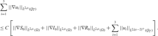(3.12) \begin{eqnarray}& & \sum_{i=1}^{3}||\nabla u_i||_{L^{2, \mu}(Q_{T})}\nonumber\\[5pt] & & \leq C\left[||\nabla S_0||_{L^{2, \mu}(\Omega)}+||\nabla I_0||_{L^{2, \mu}(\Omega)}+||\nabla R_0||_{L^{2, \mu}(\Omega)}+\sum_{i=1}^{3}||u_i||_{L^{2, (\mu-2)^+}(Q_{T})}\right].\end{eqnarray}

The $L^2(Q_{T})$ -estimate for $u_i, i=1,2,3$ implies that the above estimate holds for any $\mu\in [0,2]$ . The interpolation yields that, for any $\mu\in [0,2]$ ,

(3.13) \begin{eqnarray} \sum_{i=1}^{3}||u_i||_{L^{2,\mu+2}(Q_{T})}\leq C, \end{eqnarray}

where C depends only on known data.

Now, we go back the estimate (3.12) to see that the estimate (3.13) holds for any $\mu\in [2, 4]$ . We can continue this iteration process as long as the right-hand side of (3.9) is bounded. After a finite number of iterations, we see that the above estimate (3.12) holds for any $\mu\in [0, n)$ .

Since equation (2.3) is linear, we can use the interpolation to obtain

\[ ||u_3||_{L^{2, \mu+2}(Q_{T})}\leq C,\]

where $\mu\in [0,n)$ and C depends only on known data.

It follows that

\[ ||u_3||_{C^{\alpha, \frac{\alpha}{2}}(\bar{Q}_{T})}\leq C,\]

where C depends only on known data and $\alpha=\frac{\mu+2-n}{2}$ .

Once we have the estimate for $u_3$ in $C^{\alpha, \frac{\alpha}{2}}(\bar{Q})_{T}$ , we obtain

\[|| u_1||_{L^{\infty}(Q_{T})}\leq C.\]

Now, we can use the standard DiGorgi–Nash’s estimate to obtain

\[ ||u_1||_{C^{\alpha, \frac{\alpha}{2}}(\bar{Q})_{T})}+|u_2||_{C^{\alpha, \frac{\alpha}{2}}(\bar{Q})_{T})}\leq C,\]

where C depends only on known data.

From equation (2.4), we obtain

\[ ||u_4||_{C^{\alpha, \frac{\alpha}{2}}(\bar{Q}_{T})}\leq C,\]

where C depends only on known data.

With these estimates, the uniqueness follows immediately.

Finally, using the general theory of parabolic equations, we see that $u_i$ is smooth in $Q_T$ as long as $d_i(x,t)$ is smooth for all $i=1,2,3,4.$

4 Global bounds and asymptotic behaviour of solution

In this section, we first derive a global bound for U and then prove Theorems 2.3 and 2.4. Unlike the proof of Theorem 2.2, we must pay a special attention to various estimates which must be independent of T.

In order to see a clear physical meaning for all species, we may use the original variables (S,I,R, B) or $(u_1,u_2,u_3, u_4)$ in this section.

Lemma 4.1. Under the assumptions H(2.1)–H(2.2), there exists a constant $C_1$ such that

\begin{eqnarray*}& & \sup_{0<t<\infty}\sum_{k=1}^{4}||u_k||_{L^1(\Omega)}\leq C_1,\end{eqnarray*}

where $C_1$ depends only on know data.

Proof: We take integration over $\Omega$ for equations (2.1)–(2.3) and then add up to see

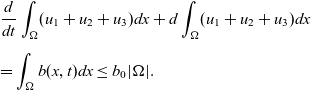\begin{eqnarray*}& & \frac{d}{dt}\int_{\Omega}(u_1+u_2+u_3)dx+d\int_{\Omega}(u_1+u_2+u_3)dx \\[5pt] & & =\int_{\Omega}b(x,t)dx \leq b_0|\Omega|.\end{eqnarray*}

Since $d>0$ , it follows that

\[ \sup_{0<t<\infty}\int_{\Omega}(u_1+u_2+u_3)dx\leq C_1,\]

where $C_1$ depends only on known data.

Now, we integrate of $\Omega$ for equation (2.1) again to find

\[ \frac{d}{dt}\int_{\Omega}u_1dx+\beta_1\int_{\Omega}u_1u_2 dx+\beta_2\int_{\Omega}u_1h(u_4)dx= \int_{\Omega}b(x,t)dx +\sigma\int_{\Omega}u_3dx.\]

It follows that

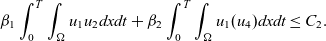\[ \beta_1\int_{0}^{T}\int_{\Omega}u_1u_2 dxdt+\beta_2\int_{0}^{T}\int_{\Omega}u_1(u_4)dxdt\leq C_2.\]

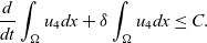
Next, we take integration over $\Omega$ for equation (2.4) to obtain

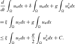\begin{eqnarray*}& & \frac{d}{dt}\int_{\Omega}u_4dx+\delta\int_{\Omega}u_4dx+g\int_{\Omega}u_{4}^2dx\\[5pt] & & =\xi \int_{\Omega}u_2dx+g\int_{\Omega}u_4 dx\\[5pt] & & \leq \xi \int_{\Omega}u_2dx+ \frac{g}{2}\int_{\Omega}u_{4}^2dx+C.\end{eqnarray*}

Since $L^1(\Omega)$ -norm of $u_2$ is uniformly bounded, it follows that

\[\frac{d}{dt}\int_{\Omega}u_4dx+\delta\int_{\Omega}u_4dx\leq C.\]

Thus, we obtain the desired $L^1(\Omega)$ -estimate for $u_4$ .

A direct consequence of Lemma 4.1 is that when the space dimension is equal to $n=1$ , from the general theory of parabolic equations (for example, See Lemma 2.6 in [Reference Caceres and Canizo5] or [Reference Bocccardo and Gallouet4]), we immediately see that S, R, I and B are uniformly bounded in Q.

When the space dimension is greater than 1, the derivation is much more complicated. In the derivation of various energy estimates, the following Young’s inequality with a small parameter $\varepsilon>0$ will be used frequently: for any $a, b\geq 0$ ,

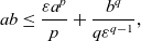\[ ab\leq \frac{\varepsilon a^{p}}{p}+\frac{b^{q}}{q\varepsilon^{q-1}},\]

where

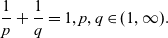\[ \frac{1}{p}+\frac{1}{q}=1, p, q \in (1, \infty).\]

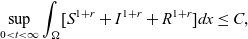
Lemma 4.2. Under the condition H(2.1)–H(2.3), there exists a constant C such that

\[ \sup_{t>0}\int_{\Omega}[S^{1+r}+I^{1+2}+R^{1+r}+B^{1+r}]dx\leq C,\]

where $r\in (0,\frac{1}{n-1})$ is arbitrary and C depends only on known data.

Proof Keep in mind that we shall always derive an estimate for S,I and R as a first step. The second step for estimating B will be followed easily once we have an estimate for I by equation (1.4).

We use the standard energy method to derive the estimate. We multiply equation (2.1) by $u_1^r$ and equation (2.3) by $R^r$ , respectively, and then integrate ove $\Omega$ to obtain

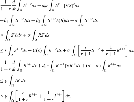\begin{eqnarray*}& & \frac{1}{1+r}\frac{d}{dt}\int_{\Omega}S^{1+r}dx +d_0r\int_{\Omega}S^{r-1}|\nabla S|^2dx\\[5pt] & & +\beta_1\int_{\Omega}S^{1+r}Idx+\beta_2\int_{\Omega}S^{1+r}h(B)dx+d\int_{\Omega}S^{1+r}dx\\[5pt] & & \leq \int_{\Omega} S^rb dx +\sigma\int_{\Omega}RS^r dx\\[5pt] & & \leq \varepsilon \int_{\Omega}S^{1+r}dx +C(\varepsilon)\int_{\Omega}b^{1+r}dx +{\sigma}\int_{\Omega}\left[\frac{r}{r+1}S^{1+r}+\frac{1}{r+1}R^{1+r}\right] dx.\\[5pt] & & \frac{1}{1+r}\frac{d}{dt}\int_{\Omega}R^{1+r}dx +d_0r\int_{\Omega}R^{r-1}|\nabla R|^2dx +(d+\sigma)\int_{\Omega}R^{1+r}dx\\[5pt] & & \leq \gamma\int_{\Omega} IR^r dx \\[5pt] & & \leq \gamma\int_{\Omega}\left[\frac{r}{1+r}R^{1+r}+\frac{1}{1+r}I^{1+r}\right] dx.\end{eqnarray*}

Similarly for I, we have

\begin{eqnarray*}& & \frac{1}{1+r}\frac{d}{dt}\int_{\Omega}I^{1+r}dx +d_0r\int_{\Omega}I^{r-1}|\nabla I|^2dx+(d+\gamma)\int_{\Omega}I^{1+r}dx\\[5pt] & & \leq \beta_1\int_{\Omega}SI^{1+r}dx+\beta_2\int_{\Omega}SI^r h(B)dx\\[5pt] & & :=J_1 +J_2.\end{eqnarray*}

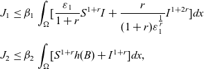\begin{eqnarray*}& & J_1\leq \beta_1\int_{\Omega}[\frac{\varepsilon_1}{1+r}S^{1+r}I +\frac{r}{(1+r)\varepsilon_1^{\frac{1}{r}}}I^{1+2r}]dx\\[5pt] & & J_2\leq \beta_2\int_{\Omega}[S^{1+r}h(B)+I^{1+r}]dx,\end{eqnarray*}

where we have used the fact $0\leq h(B)\leq 1$ for the second estimate.

We choose $\varepsilon_1=1+r$ and then add up the estimates for S,I and R to obtain

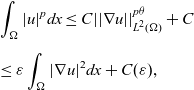
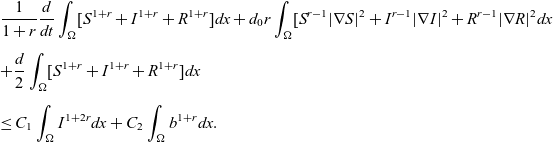\begin{eqnarray*}& & \frac{1}{1+r}\frac{d}{dt}\int_{\Omega}[S^{1+r}+I^{1+r}+R^{1+r}]dx +d_0r\int_{\Omega}[S^{r-1}|\nabla S|^2+I^{r-1}|\nabla I|^2+R^{r-1}|\nabla R|^2dx\\[5pt] & & +\frac{d}{2}\int_{\Omega}[S^{1+r}+I^{1+r}+R^{1+r}]dx\\[5pt] & & \leq C_1\int_{\Omega}I^{1+2r}dx+C_2\int_{\Omega}b^{1+r}dx.\end{eqnarray*}

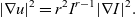
Now, we recall a Gagliardo–Nirenberg’s inequality

\[||u||_{L^{p}(\Omega)}\leq C||\nabla u||_{L^{q}(\Omega)}^{\theta}||u||_{L^{s}(\Omega)}^{1-\theta}+C||u||_{L^1} ,\]

where C depends only on n and $\Omega$ , $p, q, s, \theta$ satisfy 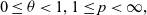$0\leq \theta<1, 1\leq p<\infty,$ and

\[ \frac{1}{p}=\theta\left(\frac{1}{q}-\frac{1}{n}\right)+(1-\theta)\frac{1}{s}.\]

We choose $q=2$ and $s=1$ , then we see that, for $p=\frac{2(1+2r)}{1+r}$ and $\theta=\frac{n(1+3r)}{(n+2)(1+2r)}$ ,

Note that by Lemma 4.1, for $u=I^{\frac{1+r}{2}}$ with $r\leq 1$ , then

\[ ||u||_{L^{1}(\Omega)}\leq C.\]

Moreover,

\[ |\nabla u|^2=r^2 I^{r-1}|\nabla I|^2.\]

If we apply Gagliardo–Nirenberg’s inequality to obtain

\begin{eqnarray*}& & \int_{\Omega}|u|^p dx\leq C||\nabla u||_{L^{2}(\Omega)}^{p\theta}+C\\\end{eqnarray*}

Note that if r satisfies

\[0<r<\frac{1}{n-1},\]

then

\[ \frac{p\theta}{2}<1.\]

We see

\begin{eqnarray*}& & \int_{\Omega}|u|^p dx\leq C||\nabla u||_{L^{2}(\Omega)}^{p\theta}+C\\[5pt] & & \leq \varepsilon\int_{\Omega}|\nabla u|^2dx +C(\varepsilon),\end{eqnarray*}

where $\varepsilon>0$ is arbitrary and $C(\varepsilon)$ depends only on $\varepsilon$ , $||u||_{L^{1}(\Omega)}$ and known data.

By choosing $\varepsilon$ sufficiently small, we obtain

\begin{eqnarray*}& & \frac{d}{dt}\int_{\Omega}[S^{1+r}+I^{1+r}+R^{1+r}]dx +\int_{\Omega}[S^{r-1}|\nabla S|^2+I^{r-1}|\nabla I|^2+R^{r-1}|\nabla R|^2dx\nonumber\\[5pt] & & +\int_{\Omega}[S^{1+r}+I^{1+r}+R^{1+r}]dx\nonumber\\[5pt] & & \leq C_3\int_{\Omega}b^{1+r}dx\leq C_3b_0^{1+r}|\Omega|.\end{eqnarray*}

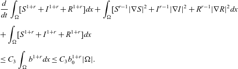
Consequently, for any $r\in (0,\frac{1}{n-1})$ , we have

\[ \sup_{0<t<\infty}\int_{\Omega}[S^{1+r}+I^{1+r}+R^{1+r}]dx\leq C,\]

where C depends only on known data.

The estimate for B follows easily from equation (1.4).

Proof of Theorem 2.3 : Let $k\geq 1$ . We follow the same calculations as in Lemma 4.2 to obtain

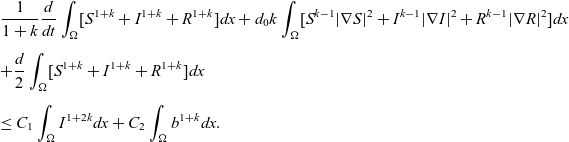\begin{eqnarray*}& & \frac{1}{1+k}\frac{d}{dt}\int_{\Omega}[S^{1+k}+I^{1+k}+R^{1+k}]dx +d_0k\int_{\Omega}[S^{k-1}|\nabla S|^2+I^{k-1}|\nabla I|^2+R^{k-1}|\nabla R|^2]dx\\[5pt] & & +\frac{d}{2}\int_{\Omega}[S^{1+k}+I^{1+k}+R^{1+k}]dx\\[5pt] & & \leq C_1\int_{\Omega}I^{1+2k}dx+C_2\int_{\Omega}b^{1+k}dx.\end{eqnarray*}

Let $u= I^{\frac{1+k}{2}}$ . As in Lemma 4.2, if we have an estimate in $L^1(\Omega)$ for a function u, then we can obtain an estimate for u in $L^{p}(\Omega)$ with $p=\frac{2n}{2n-(n+2)\theta}$ and $\theta=\frac{n(1+3k)}{(n+2)(1+2k)}$ as long as $k<\frac{1}{n-1}$ . For any $k\geq 1$ , after a finite number of steps, we obtain

\[ \sup_{t\geq 0}\int_{\Omega}[S^{1+k}+I^{1+k}+R^{1+k}]dx\leq C(k),\]

By the standard estimate for parabolic equation (see Lemma 2.6 in [Reference Caceres and Canizo5]), we obtain

\[\sup_{t\geq 0}[||S||_{L^{\infty}(\Omega}+||I||_{L^{\infty}(\Omega)}+||R||_{L^{\infty}(\Omega)}]\leq C,\]

where C depends only on known data.

Once I is uniformly bounded, we can easily derive a uniform bound for B by using the standard theory of parabolic equation ([Reference Ladyzenskaja, Solonikov and Uralceva16]). This concludes the proof of Theorem 2.3.

With the global bound for U(x,t), we are ready to prove the asymptotic behaviour of the solution for the system (1.1)–(1.6).

Proof of Theorem 2.4 : From Theorem 2.3, we have

\[ \sup_{Q}|S(x,t)|+\sup_{Q}|I(x,t)|+\sup_{Q}|R(x,t)|+\sup_{Q}|B(x,t)|\leq C,\]

where C depends only on known data.

We consider the following steady-state system corresponding to (2.1)–(2.6):

(4.1) \begin{eqnarray} -\nabla[d_{1\infty}(x)\nabla S] = b_0(x)-\beta_1SI-\beta_2S \cdot h(B)-dS+\sigma R,\end{eqnarray}

(4.2) \begin{eqnarray} -\nabla[d_{2\infty}(x)\nabla I] = \beta_1SI+\beta_2S \cdot h(B)-(d+\gamma)I,\qquad\quad \end{eqnarray}

(4.3) \begin{eqnarray} -\nabla[d_{3\infty}(x)\nabla R] = \gamma I-(d+\sigma)R,\qquad\qquad\qquad\qquad\quad \end{eqnarray}

(4.4) \begin{eqnarray} -\nabla[d_{4\infty}(x)\nabla B] = \xi I +gB(1-\frac{B}{K})-\delta B\qquad\qquad\qquad\;\; \end{eqnarray}

subject to the following boundary conditions:

(4.5) \begin{eqnarray} & & (\nabla_{\nu}S,\nabla_{\nu}I,\nabla_{\nu}R, \nabla_{\nu}B) = 0,\qquad x\in \partial \Omega, \end{eqnarray}

By using the same argument as for the system (2.1)–(2.6), we can show that the problem (4.1)–(4.5) has a weak solution $U^*(x)=(S^*(x),I^*(x),R^*(x),B^*(x))\in W_{2}^{1}(\Omega)\bigcap L^{\infty}(\Omega)$ . Moreover, since $b_0(x)\geq 0$ , the maximum principle implied that every weak solution is nonnegative on $\Omega$ . Furthermore, since the coefficients $d_{i\infty}\in C^{\alpha}(\bar{\Omega})$ , regularity theory for elliptic equation ([Reference Troianiello29]) yields

\[ ||S^*||_{C^{1+\alpha}(\bar{\Omega}}+||I^*||_{C^{1+\alpha}(\bar{\Omega}}+||R^*||_{C^{1+\alpha}(\bar{\Omega}}+||B^*||_{C^{1+\alpha}(\bar{\Omega}}\leq C,\]

where C depends only on known data.

We divide the rest of the proof into three steps. In the first step, we show that there is an upper bound $M_0$ which is independent of $\beta_1$ and $\beta_2$ . In the second step, we show that the steady-state system has a unique solution $(S_{\infty}(x), 0,0,0) $ if the parameters satisfy the conditions in Theorem 2.4, where $S_{\infty}(x)$ is a solution of (2.7)–(2.8). In the third step, we show that the U(x,t) converges to the steady-state solution $U^*(x)$ in $L^p(\Omega)$ for any $p>1$ .

Step 1. There exists a constant $M_0$ which is independent $\beta_1$ and $\beta_2$ such that

\[\sup_{\Omega}S^*(x)\leq M_0. \]

Indeed, it is easy to see

\begin{eqnarray*} & & d\int_{\Omega}[S^*+I^*+R^*]dx=\int_{\Omega}b_0(x)dx, \\[5pt] & & (\delta-g)\int_{\Omega}B^*dx+g\int_{\Omega}B^{*2}dx=\xi\int_{\Omega}I^*dx. \end{eqnarray*}

Hence, $L^1$ -bound of $(S^*,I^*,R^*,B^*)$ is independent of $\beta_1$ and $\beta_2.$ Moreover,

\[ \int_{\Omega}B^{*2}dx\leq \frac{\xi}{g}\int_{\Omega}I^*dx.\]

To derive an $L^2$ -bound, we define $V(x)=S(x)+I(x)$ . Then

(4.6) \begin{eqnarray} -\nabla[d_{1\infty}(x)\nabla S] & = & b_0(x)-\beta_1SI-\beta_2S \cdot h(B)-dS+\sigma R,\end{eqnarray}

(4.7) \begin{eqnarray} -\nabla[d_{2\infty}(x)\nabla V] & = & \nabla[(d_{1\infty}-d_{2\infty}\nabla S]+b_0(x)-dV+\sigma R, \end{eqnarray}

(4.8) \begin{eqnarray} -\nabla[d_{3\infty}(x)\nabla R] & = & \gamma I-(d+\sigma)R, \end{eqnarray}

(4.9) \begin{eqnarray} -\nabla[d_{4\infty}(x)\nabla B] & = & \xi I +gB\left(1-\frac{B}{K}\right)-\delta B,\end{eqnarray}

By using the energy method, we immediately obtain an $L^2(\Omega)$ -bound for S,V,R,B and the bound is independent $\beta_1$ and $\beta_2$ . By using the same $L^{2,\mu}$ -argument, we can deduce an $L^{\infty}(\Omega)$ bound for $S^*(x)$ and the bound is independent $\beta_1$ and $\beta_2$ .

Step 2. We show that a steady-state solution $U^*(x)$ to (4.3)–(4.7) must equal to $(S_{\infty}(x),0,0,0)$ if the conditions in Theorem 2.4 hold.

Let

\[\hat{U}(x)=(\hat{S}(x), \hat{I}(x),\hat{R}(x), \hat{B})=(S^*(x)-S_{\infty}(x), I^*(x), R^*(x), B^*(x)), x\in \Omega.\]

It is easy to see that $(\hat{S}, \hat{I}, \hat{R}, \hat{B})$ satisfies the following elliptic system (for convenience, we use $I^*,R^*,B^*$ instead of $(\hat{I},\hat{R}, \hat{B})$ ):

(4.10) \begin{eqnarray} -\nabla[d_{1\infty}(x)\nabla \hat{S}] & = & -\beta_1[\hat{S}I^*+S_{\infty}I^*]-\beta_2[\hat{S} h(B^*)+S_{\infty}h(B^*)] -d\hat{S}+\sigma R^*,\end{eqnarray}

(4.11) \begin{eqnarray} -\nabla[d_{2\infty}(x)\nabla I^*] & = & \beta_1[\hat{S}I^*+S_{\infty}I^*]+\beta_2[\hat{S}\cdot h(B^*)+S_{\infty}h(B^*)]-(d+\gamma)I^*,\end{eqnarray}

(4.12) \begin{eqnarray} -\nabla[d_{3\infty}(x)\nabla R^*] & = & \gamma I^*-(d+\sigma)R^*, \end{eqnarray}

(4.13) \begin{eqnarray} -\nabla[d_{4\infty}(x)\nabla B^*] & = & \xi I +gB^*(1-\frac{B^*}{K})-\delta B \end{eqnarray}

subject to the following boundary conditions:

(4.14) \begin{eqnarray} & & (\nabla_{\nu}\hat{S},\nabla_{\nu}I^*,\nabla_{\nu}R^*, \nabla_{\nu}B^*) = 0,\qquad x\in \partial \Omega, \end{eqnarray}

We first use $L^1(\Omega)$ -estimate to show that the steady-state system (4.6)–(4.9) with homogeneous Neumann condition has a unique solution 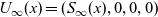$U_{\infty}(x)=(S_{\infty}(x),0,0,0)$ . From the elliptic equation (4.6), we multiply the sign function $sgn \hat{S}$ (one may use a smooth approximation of sign function first and then take the limit) to obtain the following estimates:

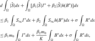(4.15) \begin{eqnarray}& & d\int_{\Omega}|\hat{S}|dx+\int_{\Omega}[\beta_1|\hat{S}|I^*+\beta_2 |\hat{S}|h(B^*)]dx \nonumber\\[5pt] & & \leq \beta_1\int_{\Omega}S_{\infty}I^*dx+\beta_2\int_{\Omega}S_{\infty}h(B^*) dx+\sigma\int_{\Omega}R^* dx\nonumber\\[5pt] & & \leq \beta_1m_0\int_{\Omega}I^{*}dx+\frac{\beta_2m_0}{K}\int_{\Omega}B^{*}dx+\sigma\int_{\Omega}R^*dx,\end{eqnarray}

where

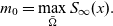\[ m_0=\max_{\bar{\Omega}}S_{\infty}(x).\]

Similarly, from equation (4.7), we have

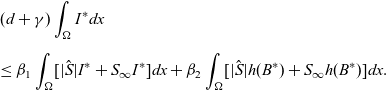(4.16) \begin{eqnarray}& & (d+\gamma)\int_{\Omega}I^{*}dx \nonumber\\[5pt] & & \leq \beta_1 \int_{\Omega}[|\hat{S}|I^*+S_{\infty}I^{*}]dx+\beta_2\int_{\Omega}[|\hat{S}|h(B^*)+S_{\infty}h(B^*)]dx. \end{eqnarray}

From equations (4.8)–(4.9), we find

(4.17) \begin{eqnarray}& & (d+\sigma)\int_{\Omega}R^{*}dx \leq \gamma\int_{\Omega} I^{*}dx.\end{eqnarray}

(4.18) \begin{eqnarray}& & (\delta-g)\int_{\Omega}B^{*}dx \leq \xi\int_{\Omega}I^{*}dx.\end{eqnarray}

We add up the estimates (4.15)–(4.17) to obtain

\begin{eqnarray*}& & d\int_{\Omega}|\hat{S}|dx +(d-2\beta_1m_0-\frac{2\beta_2m_0\xi}{K(\delta-g)})\int_{\Omega}I^{*}dx + d\int_{\Omega}R^{*}dx \leq 0,\end{eqnarray*}

where we have used the estimate (4.18) for the $L^1$ -norm of $B^*$ . If

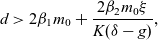\[ d>2\beta_1m_0+\frac{2\beta_2m_0\xi}{K(\delta-g)}, \]

then we conclude

\[ \hat{S}(x)=I^*(x)=R^*(x)=0,\qquad x\in \Omega.\]

Consequently, the inequality (4.18) implied $B^*(x,t)=0$ on $\Omega.$

When $d_1(x,t)$ depends on t, the above conditions for the parameters are not enough to prove U(x,t) converges to $U^*(x)$ . We need a different set of conditions on parameters to prove the uniqueness of $U^*(x)$ via $L^2$ -estimate. Indeed, we multiply equation (4.6) by $\hat{S}$ and integrate over $\Omega$ to obtain

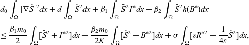(4.19) \begin{eqnarray}& & d_0\int_{\Omega}|\nabla \hat{S}|^2dx+d\int_{\Omega}\hat{S}^2dx+\beta_1\int_{\Omega}\hat{S}^2I^*dx +\beta_2\int_{\Omega}\hat{S}^2h(B^*)dx\nonumber\\[5pt] & & \leq \frac{\beta_1m_0}{2}\int_{\Omega}[\hat{S}^2+I^{*2}]dx+\frac{\beta_2m_0}{2K}\int_{\Omega}[\hat{S}^2+B^{*2}]dx+\sigma\int_{\Omega}[\varepsilon R^{*2}+\frac{1}{4\varepsilon}\hat{S}^2]dx,\end{eqnarray}

where we have used fact $h(B^*)\leq \frac{B^*}{K}$ and Cauchy–Schwarz’s inequality with a parameter $\varepsilon>0$ .

Similarly, from equation (4.7), we have

(4.20) \begin{eqnarray}& & d_0\int_{\Omega}|\nabla I^*|^2dx+(d+\gamma)\int_{\Omega}I^{*2}dx \leq \beta_1M_0\int_{\Omega}I^{*2}dx+\frac{\beta_2M_0}{2K}\int_{\Omega}[I^{*2}+B^{*2}]dx,\end{eqnarray}

From equations (4.8)–(4.9), we find

(4.21) \begin{eqnarray}& & d_0\int_{\Omega}|\nabla R^*|^2dx+(d+\sigma)\int_{\Omega}R^{*2}dx\leq \gamma\int_{\Omega}[\varepsilon I^{*2}+\frac{1}{4\varepsilon}R^{*2}]dx;\end{eqnarray}

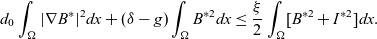(4.22) \begin{eqnarray}& & d_0\int_{\Omega}|\nabla B^*|^2dx+(\delta-g)\int_{\Omega}B^{*2}dx\leq \frac{\xi}{2}\int_{\Omega}[ B^{*2}+I^{*2}]dx.\end{eqnarray}

From the estimate (4.18), we see

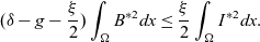\[ (\delta-g-\frac{\xi}{2})\int_{\Omega}B^{*2}dx\leq\frac{\xi}{2}\int_{\Omega}I^{*2}dx.\]

If we combine the estimates (4.15)–(4.18) and choose $\varepsilon$ sufficiently close to 1 to conclude that

\[ \hat{S}(x)=I^*(x)=R^*(x)=0,\qquad x\in \Omega\]

provided that

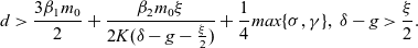\[ d>\frac{3\beta_1m_0}{2}+\frac{\beta_2m_0\xi}{2K(\delta-g-\frac{\xi}{2})}+\frac{1}{4}max\{\sigma, \gamma\},\, \delta-g>\frac{\xi}{2}. \]

The inequality (4.18) yields

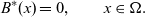\[ B^*(x)=0,\qquad x\in \Omega.\]

That is

\[ U^*(x)=(S_{\infty}(x),0,0,0),\qquad x\in \Omega.\]

Consequently, $M_0=m_0$ .

Step 3: In this step, we show that U(x,t) converges to the steady-state solution $U^*(x)=(S_{\infty}(x),0,0,0)$ as $t\rightarrow \infty$ .

For convenience, we set

\[ W(x,t):=(w_1, w_2, w_3, w_4)= U(x,t)-U^*(x)=(S-S_{\infty},I,R, B), (x,t)\in Q.\]

A direct calculation shows that W(x,t) satisfies the following system:

(4.23) \begin{eqnarray}& & w_{1t}-\nabla[d_1(x,t)\nabla w_1]=m_1(x,t)+f_1(x,t,U)-f_1(x,U^*), (x,t)\in Q,\end{eqnarray}

(4.24) \begin{eqnarray} & & w_{2t}-\nabla[d_2(x,t)\nabla w_2]=m_2(x,t)+f_2(U)-f_2(U^*),\quad (x,t)\in Q, \end{eqnarray}

(4.25) \begin{eqnarray}& & w_{3t}-\nabla[d_3(x,t)\nabla w_3]=m_3(x,t)+f_3(U)-f_3(U^*),\quad (x,t)\in Q,\end{eqnarray}

(4.26) \begin{eqnarray} & & w_{4t}-\nabla[d_4(x,t)\nabla w_4]=m_4(x,t)+f_4(U)-f_4(U^*),\quad (x,t)\in Q, \end{eqnarray}

subject to the boundary conditions:

(4.27) \begin{eqnarray} & & \nabla_{\nu}(w_1,w_2,w_3,w_4)=0,\qquad (x,t)\in \partial \Omega\times (0,\infty),\end{eqnarray}

where

\[ m_i(x,t)=\nabla[(d_i(x,t)-d_{i\infty}(x))\nabla u_{i}^{*}], i=1, \cdots, 4.\]

When $d_i(x,t)$ is independent of t, we see $m_i(x,t)=0$ in Q. For this case, we can use the same method as in Step 2 to show that W(x,t) converges to $U^*(x)$ in $L^1(\Omega)$ if the conditions in Step 2 hold.

Now, we consider the general case when $d_i$ depends on t. Note that $d_{i\infty}(x)$ are uniformly bounded in $C^{\alpha}(\bar{\Omega})$ , we know that $\nabla u_i^*$ is uniformly bounded in $\Omega$ . Hence, for each i,

\[|\int_{\Omega}m_i(x) w_i dx|\leq \varepsilon_1\int_{\Omega}|\nabla w_i|^2dx+C(\varepsilon_1)\int_{\Omega}(d_i-d_{i\infty})^2dx,\]

where $\varepsilon_1$ is a small parameter.

For any $t_0>0$ . Let $Q(t_0)=\Omega\times [t_0,\infty)$ and

\[ m_0^*=\sup_{Q(t_0)}s^*(x,t).\]

By using the same argument as in Step 1, we see $m_0^*$ is independent of $\beta_1$ and $\beta_2$ .

Observe $h(0)=0$ , hence

\begin{eqnarray*}& & f_1(x,t,U)-f_1(x,U^*)\\[5pt] & & =b(x,t)-b_0(x)-\beta_1[w_1w_2+S_{\infty}w_2]-\beta_2[w_1h(B)+S_{\infty}(h(B))]-d w_1+\sigma w_3.\end{eqnarray*}

Moreover, from the definition of h(B),

\[ |h(B)|\leq \frac{|w_4|}{K}.\]

It follows that

\begin{eqnarray*}& & |w_1 S_{\infty}w_2|\leq \frac{m_0}{2}[w_1^2+w_2^2];\\[5pt] & & |w_1S_{\infty}h(w_4)|\leq \frac{m_0}{2K}(w_1^2+w_4^2).\end{eqnarray*}

Now, we use the standard energy estimate to obtain

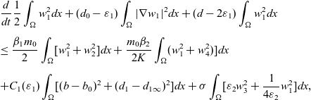\begin{eqnarray*} & & \frac{d}{dt}\frac{1}{2}\int_{\Omega}w_1^2dx +(d_0-\varepsilon_1)\int_{\Omega}|\nabla w_1|^2dx+(d-2\varepsilon_1)\int_{\Omega}w_1^2dx\\[5pt] & & \leq \frac{\beta_1m_0}{2}\int_{\Omega}[w_1^2+w_2^2]dx+\frac{m_0\beta_2}{2K}\int_{\Omega}(w_1^2+w_4^2)]dx\\[5pt] & & + C_1(\varepsilon_1)\int_{\Omega}[(b-b_0)^2+(d_1-d_{1\infty})^2]dx+\sigma\int_{\Omega}[\varepsilon_2 w_3^2+\frac{1}{4\varepsilon_2}w_1^2]dx, \end{eqnarray*}

where $\varepsilon_1$ and $\varepsilon_2$ are arbitrarily constants.

Similarly, since $f_2(U^*)=f_3(U^*)=f_4(U^*)=0$ , we have

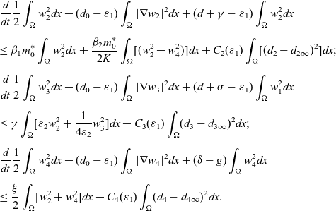\begin{eqnarray*} & & \frac{d}{dt}\frac{1}{2}\int_{\Omega}w_2^2dx +(d_0-\varepsilon_1)\int_{\Omega}|\nabla w_2|^2dx+(d+\gamma-\varepsilon_1)\int_{\Omega}w_2^2dx\\[5pt] & & \leq \beta_1m_0^*\int_{\Omega}w_2^2dx+\frac{\beta_2m_0^*}{2K}\int_{\Omega}[(w_2^2+w_4^2)]dx+ C_2(\varepsilon_1)\int_{\Omega}[(d_2-d_{2\infty})^2]dx;\\[5pt] & & \frac{d}{dt}\frac{1}{2}\int_{\Omega}w_3^2dx +(d_0-\varepsilon_1)\int_{\Omega}|\nabla w_3|^2dx+(d+\sigma-\varepsilon_1)\int_{\Omega}w_1^2dx\\[5pt] & & \leq \gamma\int_{\Omega}[\varepsilon_2 w_2^2+\frac{1}{4\varepsilon_2}w_3^2]dx+C_3(\varepsilon_1)\int_{\Omega}(d_{3}-d_{3\infty})^2dx;\\[5pt] & & \frac{d}{dt}\frac{1}{2}\int_{\Omega}w_4^2dx +(d_0-\varepsilon_1)\int_{\Omega}|\nabla w_4|^2dx+(\delta-g)\int_{\Omega}w_4^2dx\\[5pt] & & \leq \frac{\xi}{2}\int_{\Omega}[w_2^2+w_4^2]dx+C_4(\varepsilon_1)\int_{\Omega}(d_4-d_{4\infty})^2dx. \end{eqnarray*}

Suppose the parameters in the system (1.1)–(1.4) satisfy the following conditions:

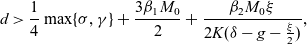(4.28) \begin{eqnarray} & & d>\frac{1}{4}\max\{ \sigma, \gamma\}+ \frac{3\beta_1M_0}{2}+\frac{\beta_2M_0\xi}{2K(\delta-g-\frac{\xi}{2})}, \end{eqnarray}

(4.29) \begin{eqnarray} & & \delta-g>\frac{\xi}{2}, \end{eqnarray}

where 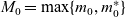$M_0=\max\{m_0, m_0^*\}$ .

We choose $\varepsilon_1$ sufficiently small and $\varepsilon_2$ sufficiently close to 1, then we combine the above estimates to see that there exists a constant $\alpha_1>0$ such that

\[ Y'(t)+\alpha_1 Y(t)\leq C G(t),\]

where

\[ Y(t)=\sum_{i=1}^{4}\int_{\Omega}w_i^2dx, G(t)=\int_{\Omega}[(b-b_0)^2+\sum_{i=1}^{4}(d_i-d_{i\infty})^2]dx.\]

Since G(t) converges to 0 as $\rightarrow \infty$ , we conclude that

\[ \lim_{t\rightarrow \infty}Y(t)=0,\]

which implies, for any $p>1$ ,

\[ \lim_{t\rightarrow \infty}||U-U^*||_{L^{p}(\Omega)}=0\]

since U(x,t) and $U^*(x)$ are uniformly bounded.

Finally, we can choose $m_0^*$ sufficiently close to $m_0$ as long as $t_0$ is sufficiently large. Therefore, the convergence of U(x,t) to $U^*(x)$ holds if the conditions for parameters in Theorem 2.4 hold.

The proof of Theorem 2.4 is completed.

5 Conclusion

In this paper, we studied a mathematical model for the Cholera epidemic without lifetime immunity. The model equations are governed by a coupled reaction–diffusion system with different diffusion coefficients for each species. We established the global well-posedness for the coupled reaction–diffusion system under a certain condition on known data. Moreover, the long-time behaviour of the solution is obtained for any space dimension n. Particularly, we prove that there is a global attractor for the system under appropriate conditions on known data. These results justify the mathematical model and provide scientists a deeper understanding of the dynamics of interaction between bacteria and susceptible, infected and recovered human hosts. The mathematical model with the help of real data analysis provides a scientific foundation for policymakers to make better decisions for the general public in health and medical sciences. The main tools used in this paper come from some delicate theories for elliptic and parabolic equations. The method developed in this paper can be used to study other models such as the avian influenza for birds.