1 Introduction
In modern gas turbine combustors, the swirl component of mean flow is intended to provide improved mixing and flame anchoring via development of appropriate recirculation zones (e.g. Candel et al.
Reference Candel, Durox, Schuller, Bourgouin and Moeck2014), while e.g. as the swirl intensity crosses a certain threshold at low to moderate Reynolds numbers (
 $Re$
), these reverse flow regions that start at a breakdown bubble (which itself can be unstable at higher
$Re$
), these reverse flow regions that start at a breakdown bubble (which itself can be unstable at higher
 $Re$
) are eventually closed at the downstream end. Such flows have the distinct potential for newer types of hydrodynamic instabilities, beyond the classical helical and double-helical ones (see Escudier Reference Escudier1988; Billant, Chomaz & Huerre Reference Billant, Chomaz and Huerre1998; Ruith et al.
Reference Ruith, Chen, Meiburg and Maxworthy2003; Liang & Maxworthy Reference Liang and Maxworthy2005; Gallaire et al.
Reference Gallaire, Ruith, Meiburg, Chomaz and Huerre2006), e.g. non-modal transient instabilities, which we explore here. These flows are characterized by a transition from an initial jet-like profile (more correctly, a ring jet with the recirculation region at its core, see e.g. Oberleithner et al.
Reference Oberleithner, Sieber, Nayeri, Paschereit, Petz, Hege, Noack and Wygnanski2011) to a wake-like profile as the recirculation bubble collapses via the appearance of a stagnation point. Although the inherent multi-dimensional nature of such flows involving recirculation zones, twin shear layers and the associated shear forces in different directions may appear complex, in most cases, a two-dimensional axisymmetric analysis is more than sufficient to compute the associated stability states.
$Re$
) are eventually closed at the downstream end. Such flows have the distinct potential for newer types of hydrodynamic instabilities, beyond the classical helical and double-helical ones (see Escudier Reference Escudier1988; Billant, Chomaz & Huerre Reference Billant, Chomaz and Huerre1998; Ruith et al.
Reference Ruith, Chen, Meiburg and Maxworthy2003; Liang & Maxworthy Reference Liang and Maxworthy2005; Gallaire et al.
Reference Gallaire, Ruith, Meiburg, Chomaz and Huerre2006), e.g. non-modal transient instabilities, which we explore here. These flows are characterized by a transition from an initial jet-like profile (more correctly, a ring jet with the recirculation region at its core, see e.g. Oberleithner et al.
Reference Oberleithner, Sieber, Nayeri, Paschereit, Petz, Hege, Noack and Wygnanski2011) to a wake-like profile as the recirculation bubble collapses via the appearance of a stagnation point. Although the inherent multi-dimensional nature of such flows involving recirculation zones, twin shear layers and the associated shear forces in different directions may appear complex, in most cases, a two-dimensional axisymmetric analysis is more than sufficient to compute the associated stability states.
A significant amount of past research has been directed to uncover any universal mechanism behind vortex breakdown in swirling flows, either axisymmetric or spiral, and the connection to its stability state, where it seems that the nature of inlet velocity profile plays an important role (e.g. Liang & Maxworthy Reference Liang and Maxworthy2005), as does the degree of swirl
 $S$
, a parameter representing the ratio between the axial components of azimuthal and axial momentums (e.g. Oberleithner et al.
Reference Oberleithner, Sieber, Nayeri, Paschereit, Petz, Hege, Noack and Wygnanski2011) and the corresponding
$S$
, a parameter representing the ratio between the axial components of azimuthal and axial momentums (e.g. Oberleithner et al.
Reference Oberleithner, Sieber, Nayeri, Paschereit, Petz, Hege, Noack and Wygnanski2011) and the corresponding
 $Re$
(in this context, see also the mode selection scenarios discussed in Gallaire & Chomaz Reference Gallaire and Chomaz2003, for a pre-breakdown jet). The axisymmetric vortex breakdown is sometimes simply attributed to a change in flow criticality (e.g. Benjamin Reference Benjamin1962; Escudier Reference Escudier1988; Liang & Maxworthy Reference Liang and Maxworthy2008). However, at higher swirl numbers helical modes outside the bubble take over and a major focus in the past has been to identify whether a pocket of absolutely unstable flow could be directly linked to this bubble collapse via higher-order spiral breakdown states (see e.g. Billant et al.
Reference Billant, Chomaz and Huerre1998; Ruith et al.
Reference Ruith, Chen, Meiburg and Maxworthy2003; Liang & Maxworthy Reference Liang and Maxworthy2005; Gallaire et al.
Reference Gallaire, Ruith, Meiburg, Chomaz and Huerre2006). In this context, Gallaire et al. (Reference Gallaire, Ruith, Meiburg, Chomaz and Huerre2006) found two such locations of absolute instability: one inside the bubble, while a second one developed inside the wake downstream of the bubble, with an analysis that concluded spiral breakdown to be driven by the global frequency of the convective to absolute transition at the latter location. This contrasts the finding of Qadri, Mistry & Juniper (Reference Qadri, Mistry and Juniper2013), who discovered, via investigating the structural sensitivity of the spiral mode, the flow around the bubble to be more sensitive to feedback and hence must be the possible location of a wavemaker region. Others have also proposed this spiral breakdown to be initiated inside the recirculation bubble (e.g. Billant et al.
Reference Billant, Chomaz and Huerre1998; Liang & Maxworthy Reference Liang and Maxworthy2005). Although from these analyses it appears that absolute/convective instability concepts based on modal analysis provide a convincing picture of the final unsteady structures of swirling flows, the onset of such instabilities as the flow develops in time remains unknown. Whether short-time transient growths are strong enough to nonlinearly enhance the exponential growths from the corresponding modes, thereby yielding a final instability state due to a multi-mode mechanism, is yet to be explored in a measured swirling jet, which is one of the motivations behind this study. Here we note that in the related Batchelor vortex model of swirling flows, strong transient growths have indeed been observed (see Schmid et al.
Reference Schmid, Henningson, Khorrami and Malik1993; Ben-Dov, Levinski & Cohen Reference Ben-Dov, Levinski and Cohen2004) at parametric spaces where strong modal growths also co-exist. Further, considering the fact that typical swirling flows encompass large parametric spaces with multiple tuning parameters, it is possible for such non-modal growths to be more relevant over certain parametric configurations to yield some sort of a ‘bypass’ mechanism in reaching a breakdown state (for similar discussions on Batchelor vortex, see Heaton & Peake Reference Heaton and Peake2007).
$Re$
(in this context, see also the mode selection scenarios discussed in Gallaire & Chomaz Reference Gallaire and Chomaz2003, for a pre-breakdown jet). The axisymmetric vortex breakdown is sometimes simply attributed to a change in flow criticality (e.g. Benjamin Reference Benjamin1962; Escudier Reference Escudier1988; Liang & Maxworthy Reference Liang and Maxworthy2008). However, at higher swirl numbers helical modes outside the bubble take over and a major focus in the past has been to identify whether a pocket of absolutely unstable flow could be directly linked to this bubble collapse via higher-order spiral breakdown states (see e.g. Billant et al.
Reference Billant, Chomaz and Huerre1998; Ruith et al.
Reference Ruith, Chen, Meiburg and Maxworthy2003; Liang & Maxworthy Reference Liang and Maxworthy2005; Gallaire et al.
Reference Gallaire, Ruith, Meiburg, Chomaz and Huerre2006). In this context, Gallaire et al. (Reference Gallaire, Ruith, Meiburg, Chomaz and Huerre2006) found two such locations of absolute instability: one inside the bubble, while a second one developed inside the wake downstream of the bubble, with an analysis that concluded spiral breakdown to be driven by the global frequency of the convective to absolute transition at the latter location. This contrasts the finding of Qadri, Mistry & Juniper (Reference Qadri, Mistry and Juniper2013), who discovered, via investigating the structural sensitivity of the spiral mode, the flow around the bubble to be more sensitive to feedback and hence must be the possible location of a wavemaker region. Others have also proposed this spiral breakdown to be initiated inside the recirculation bubble (e.g. Billant et al.
Reference Billant, Chomaz and Huerre1998; Liang & Maxworthy Reference Liang and Maxworthy2005). Although from these analyses it appears that absolute/convective instability concepts based on modal analysis provide a convincing picture of the final unsteady structures of swirling flows, the onset of such instabilities as the flow develops in time remains unknown. Whether short-time transient growths are strong enough to nonlinearly enhance the exponential growths from the corresponding modes, thereby yielding a final instability state due to a multi-mode mechanism, is yet to be explored in a measured swirling jet, which is one of the motivations behind this study. Here we note that in the related Batchelor vortex model of swirling flows, strong transient growths have indeed been observed (see Schmid et al.
Reference Schmid, Henningson, Khorrami and Malik1993; Ben-Dov, Levinski & Cohen Reference Ben-Dov, Levinski and Cohen2004) at parametric spaces where strong modal growths also co-exist. Further, considering the fact that typical swirling flows encompass large parametric spaces with multiple tuning parameters, it is possible for such non-modal growths to be more relevant over certain parametric configurations to yield some sort of a ‘bypass’ mechanism in reaching a breakdown state (for similar discussions on Batchelor vortex, see Heaton & Peake Reference Heaton and Peake2007).
In this work, our goal is therefore to investigate whether important transient growths (compared to exponential modal growths) can exist in a strongly swirling (
 $S=1.22$
) high Reynolds number (
$S=1.22$
) high Reynolds number (
 $Re_{D}=20\,000$
) jet that has undergone an axisymmetric bubble breakdown (as measured by Oberleithner et al.
Reference Oberleithner, Sieber, Nayeri, Paschereit, Petz, Hege, Noack and Wygnanski2011), a case for which global instability at a specific frequency is known to exist. In a temporal framework, we ascertain whether certain combinations of streamwise wavenumber
$Re_{D}=20\,000$
) jet that has undergone an axisymmetric bubble breakdown (as measured by Oberleithner et al.
Reference Oberleithner, Sieber, Nayeri, Paschereit, Petz, Hege, Noack and Wygnanski2011), a case for which global instability at a specific frequency is known to exist. In a temporal framework, we ascertain whether certain combinations of streamwise wavenumber
 $\unicode[STIX]{x1D6FC}$
and azimuthal wavenumber
$\unicode[STIX]{x1D6FC}$
and azimuthal wavenumber
 $m$
are more favourable for non-modal growths to appear, while at the same time analysing how it differentially affects portions of the swirling flow, including the recirculation bubble region and the wake downstream by particularly focusing on their respective growth mechanisms. In this context, we note here that a large body of classical work exists on non-modal transient analysis in bounded and semi-unbounded flows (see e.g. Reddy & Henningson Reference Reddy and Henningson1993; Andersson, Berggren & Henningson Reference Andersson, Berggren and Henningson1999; Schmid Reference Schmid2000; Schmid & Henningson Reference Schmid and Henningson2001; Akervik et al.
Reference Akervik, Hoepffner, Ehrenstein and Henningson2007), while for open flows like jets and mixing layers such studies have appeared only more recently (e.g. Nichols & Lele Reference Nichols and Lele2011; Arratia, Caulfield & Chomaz Reference Arratia, Caulfield and Chomaz2013; Garnaud et al.
Reference Garnaud, Lesshafft, Schmid and Huerre2013; Vitoshkin & Gelfgat Reference Vitoshkin and Gelfgat2014). For the first class of simple bounded flows (see Couette, pipe, channel, etc.), modal analysis predicts the flow either to be stable or unstable at higher Reynolds numbers (compared to experimental measurements), so for these flows to reach turbulent states via short-time transient growths appears unambiguous. In contrast for shear flows, unstable exponential modes are present that dominate the large-time dynamics. Here, how the short-time transient gains may fit into the overall flow instability picture is quite unclear. Moreover, any non-normality is usually regarded as unimportant at the lower
$m$
are more favourable for non-modal growths to appear, while at the same time analysing how it differentially affects portions of the swirling flow, including the recirculation bubble region and the wake downstream by particularly focusing on their respective growth mechanisms. In this context, we note here that a large body of classical work exists on non-modal transient analysis in bounded and semi-unbounded flows (see e.g. Reddy & Henningson Reference Reddy and Henningson1993; Andersson, Berggren & Henningson Reference Andersson, Berggren and Henningson1999; Schmid Reference Schmid2000; Schmid & Henningson Reference Schmid and Henningson2001; Akervik et al.
Reference Akervik, Hoepffner, Ehrenstein and Henningson2007), while for open flows like jets and mixing layers such studies have appeared only more recently (e.g. Nichols & Lele Reference Nichols and Lele2011; Arratia, Caulfield & Chomaz Reference Arratia, Caulfield and Chomaz2013; Garnaud et al.
Reference Garnaud, Lesshafft, Schmid and Huerre2013; Vitoshkin & Gelfgat Reference Vitoshkin and Gelfgat2014). For the first class of simple bounded flows (see Couette, pipe, channel, etc.), modal analysis predicts the flow either to be stable or unstable at higher Reynolds numbers (compared to experimental measurements), so for these flows to reach turbulent states via short-time transient growths appears unambiguous. In contrast for shear flows, unstable exponential modes are present that dominate the large-time dynamics. Here, how the short-time transient gains may fit into the overall flow instability picture is quite unclear. Moreover, any non-normality is usually regarded as unimportant at the lower
 $Re$
(see e.g. Qadri et al.
Reference Qadri, Mistry and Juniper2013), but as the advection effects grow at higher
$Re$
(see e.g. Qadri et al.
Reference Qadri, Mistry and Juniper2013), but as the advection effects grow at higher
 $Re$
this is presumed important (Chomaz Reference Chomaz2005), as we will show for the relatively higher
$Re$
this is presumed important (Chomaz Reference Chomaz2005), as we will show for the relatively higher
 $Re$
(compared to other existing studies) swirling jet considered here. Nevertheless, it is always possible for the collective growth from algebraic modes to be important at shorter times, as has been observed for the Batchelor and Lamb–Oseen vortex models of swirling flow (Antkowiak & Brancher Reference Antkowiak and Brancher2004; Pradeep & Hussain Reference Pradeep and Hussain2006; Heaton Reference Heaton2007; Fontane, Brancher & Fabre Reference Fontane, Brancher and Fabre2008; Mao & Sherwin Reference Mao and Sherwin2012), so that such transient perturbations, if allowed to reach finite amplitudes, may yield non-trivial modifications of the underlying mean flow to fundamentally alter its primary instability character.
$Re$
(compared to other existing studies) swirling jet considered here. Nevertheless, it is always possible for the collective growth from algebraic modes to be important at shorter times, as has been observed for the Batchelor and Lamb–Oseen vortex models of swirling flow (Antkowiak & Brancher Reference Antkowiak and Brancher2004; Pradeep & Hussain Reference Pradeep and Hussain2006; Heaton Reference Heaton2007; Fontane, Brancher & Fabre Reference Fontane, Brancher and Fabre2008; Mao & Sherwin Reference Mao and Sherwin2012), so that such transient perturbations, if allowed to reach finite amplitudes, may yield non-trivial modifications of the underlying mean flow to fundamentally alter its primary instability character.
In this context, we note that the local stability approach followed here is of a quasi-laminar nature (e.g. Mettot, Sipp & Bézard Reference Mettot, Sipp and Bézard2014), where molecular viscosity is used in the viscous terms of the governing equations, further linearized about the turbulent mean obtained from the experiments of Oberleithner et al. (Reference Oberleithner, Sieber, Nayeri, Paschereit, Petz, Hege, Noack and Wygnanski2011). However, it is also possible to include a turbulence model equation, e.g. unsteady RANS (URANS), along with our governing equations, both linearized about a fixed point of the former to yield stability equations for a fully turbulent flow (Crouch, Garbaruk & Magidov Reference Crouch, Garbaruk and Magidov2007; Meliga, Pujals & Serre Reference Meliga, Pujals and Serre2012). Alternatively, an easier option is to simply extract a spatially varying turbulent eddy viscosity from the nonlinear stresses, if available, which can be used with the viscous terms of the stability equations, in addition to the molecular viscosity (Tammisola & Juniper Reference Tammisola and Juniper2016). This last approach reduces the effective
 $Re$
of the flow, especially in regions where turbulence kinetic energy is high, providing improved agreement of global mode shapes (see Tammisola & Juniper Reference Tammisola and Juniper2016) that appears to be attractive. Unfortunately, most models of eddy viscosity are known to overestimate the turbulent dissipation, thereby markedly stabilizing the exponential growth of the leading modes. In our work, it can be particularly problematic as this would automatically increase the relative importance of the non-modal algebraic modes via artificial overdamping of the exponentially growing modal spectrum at most streamwise locations, unless the algebraic modes are also equally damped. In the absence of adequate clarity on the role of turbulent eddy viscosity models on the growth rates of, especially, the algebraic modes of the swirling jet spectrum, our preference is for a quasi-laminar approach via using a uniform molecular viscosity.
$Re$
of the flow, especially in regions where turbulence kinetic energy is high, providing improved agreement of global mode shapes (see Tammisola & Juniper Reference Tammisola and Juniper2016) that appears to be attractive. Unfortunately, most models of eddy viscosity are known to overestimate the turbulent dissipation, thereby markedly stabilizing the exponential growth of the leading modes. In our work, it can be particularly problematic as this would automatically increase the relative importance of the non-modal algebraic modes via artificial overdamping of the exponentially growing modal spectrum at most streamwise locations, unless the algebraic modes are also equally damped. In the absence of adequate clarity on the role of turbulent eddy viscosity models on the growth rates of, especially, the algebraic modes of the swirling jet spectrum, our preference is for a quasi-laminar approach via using a uniform molecular viscosity.
In shear flows, the transient growth of perturbations is usually attributed to two classical inviscid theories: the Orr mechanism (Orr Reference Orr1907) and the lift-up mechanism (see Landahl Reference Landahl1980; Butler & Farrell Reference Butler and Farrell1992). In the former, initially spanwise vortices are kinematically deformed due to the base-flow mean shear, which owing to their reorientation toward the direction of maximum stretching get energetically amplified, while in the latter mechanism streamwise vortices are perturbed via their interaction with this mean shear. In vortical flows, Antkowiak & Brancher (Reference Antkowiak and Brancher2004) found the presence of a ‘core-contamination’ mechanism, which in essence is a combination of the advection and unfolding effects of vortex spirals, analogous to the inviscid Orr mechanism, followed by velocity induction at the vortex core. Another process specific to vortical flows, as identified by Antkowiak & Brancher (Reference Antkowiak and Brancher2007) for axisymmetric amplifications, is referred to ‘anti-lift-up’ to contrast the lift-up mechanism in plane shear flows. In the former, optimal initial perturbations in the form of streamwise azimuthal velocity streaks are shown to evolve into streamwise rolls or vortex rings. Since similar evolution mechanisms are also evidenced in Batchelor vortex flows (see Mao & Sherwin Reference Mao and Sherwin2012), quite naturally, the question arises whether such idealized mechanisms could be identified in experimentally measured swirling flows with streamwise variations, like we consider here. In fact, we show that the strong and contrasting nature of transient growths that we observe in our swirling mean flow could indeed be explained by focusing on these optimal perturbation mechanisms, where the imposed wavenumbers select one of these optimal mechanisms that further depends upon the corresponding streamwise location.
To quantify transient amplifications, we perform a series of local analyses on the time-averaged mean flow, as extracted from the axisymmetric bubble and its wake of the relatively higher-
 $Re$
, strongly swirling post-breakdown jet, as measured by Oberleithner et al. (Reference Oberleithner, Sieber, Nayeri, Paschereit, Petz, Hege, Noack and Wygnanski2011). Of course, the parallel (or quasi-parallel) assumption that is inherent in such local analyses may be questioned (see e.g. Gallaire et al.
Reference Gallaire, Ruith, Meiburg, Chomaz and Huerre2006), especially at the upstream and downstream edges of the recirculation bubble, but at a few jet diameters downstream in the wake region and, perhaps, near the centre of the bubble where the streamlines are nearly parallel (see figure 2 of Oberleithner et al.
Reference Oberleithner, Sieber, Nayeri, Paschereit, Petz, Hege, Noack and Wygnanski2011), local solutions can be fairly accurate. It is later shown in this work that the mean flow non-parallelism and its effect on the respective transient growth can be qualified via noting the relative smoothness of the maximum transient growth variation along the streamwise direction. At higher times, this procedure clearly identifies three distinct regions within which this maximum growth curve can be smoothly varying, where the effect of flow non-parallelism is thus minimal. One such region is at the core of the recirculation bubble, away from the edges, while the other two are located inside the wake. Here, we mention that a fully global transient analysis using a reconstructed, continuously varying base flow, via interpolating the available discrete data, is also possible, although not explored here. However, a similar global transient analysis of Batchelor vortex by Mao & Sherwin (Reference Mao and Sherwin2012), found answers that are not qualitatively dissimilar from a corresponding local analysis. The strong transient growths from the respective continuous spectra that our present local analysis confirms at several streamwise locations are also expected to be qualitatively unaltered even for a fully global approach.
$Re$
, strongly swirling post-breakdown jet, as measured by Oberleithner et al. (Reference Oberleithner, Sieber, Nayeri, Paschereit, Petz, Hege, Noack and Wygnanski2011). Of course, the parallel (or quasi-parallel) assumption that is inherent in such local analyses may be questioned (see e.g. Gallaire et al.
Reference Gallaire, Ruith, Meiburg, Chomaz and Huerre2006), especially at the upstream and downstream edges of the recirculation bubble, but at a few jet diameters downstream in the wake region and, perhaps, near the centre of the bubble where the streamlines are nearly parallel (see figure 2 of Oberleithner et al.
Reference Oberleithner, Sieber, Nayeri, Paschereit, Petz, Hege, Noack and Wygnanski2011), local solutions can be fairly accurate. It is later shown in this work that the mean flow non-parallelism and its effect on the respective transient growth can be qualified via noting the relative smoothness of the maximum transient growth variation along the streamwise direction. At higher times, this procedure clearly identifies three distinct regions within which this maximum growth curve can be smoothly varying, where the effect of flow non-parallelism is thus minimal. One such region is at the core of the recirculation bubble, away from the edges, while the other two are located inside the wake. Here, we mention that a fully global transient analysis using a reconstructed, continuously varying base flow, via interpolating the available discrete data, is also possible, although not explored here. However, a similar global transient analysis of Batchelor vortex by Mao & Sherwin (Reference Mao and Sherwin2012), found answers that are not qualitatively dissimilar from a corresponding local analysis. The strong transient growths from the respective continuous spectra that our present local analysis confirms at several streamwise locations are also expected to be qualitatively unaltered even for a fully global approach.
The remaining paper is organized as follows. In § 2, a brief description of the underlying base flow as extracted from Oberleithner et al. (Reference Oberleithner, Sieber, Nayeri, Paschereit, Petz, Hege, Noack and Wygnanski2011) is given. Some highlights of our linear stability solver along with the local transient analysis is in § 3. Section 4 classifies the linear stability spectrum, which also motivates the pseudospectrum analysis, as introduced in this section. The main results are in § 5, where §§ 5.2, 5.3 and 5.4 focus on establishing the dynamically important transient amplifications inside the wake region, while § 5.5 deals with the corresponding optimal energy growth mechanisms. The paper is concluded via § 6, while appendix A documents more parametric details of the transient calculations and appendix B lists matrix terms of the eigenvalue problem.
2 The mean flow
The mean flow as extracted from the measurements of Oberleithner et al. (Reference Oberleithner, Sieber, Nayeri, Paschereit, Petz, Hege, Noack and Wygnanski2011) for a turbulent swirling free jet of
 $Re_{D}=20\,000$
and
$Re_{D}=20\,000$
and
 $S=1.22$
is shown in figure 1. Here,
$S=1.22$
is shown in figure 1. Here,
 $Re_{D}$
is the Reynolds number based on the nozzle diameter
$Re_{D}$
is the Reynolds number based on the nozzle diameter
 $D^{\ast }$
and average axial velocity
$D^{\ast }$
and average axial velocity
 $U^{\ast }$
, with
$U^{\ast }$
, with
 $(\,)^{\ast }$
denoting dimensional quantities, while the swirl number
$(\,)^{\ast }$
denoting dimensional quantities, while the swirl number
 $S$
is the ratio between the axial fluxes of angular and axial momentum, which does not vary along the streamwise direction.
$S$
is the ratio between the axial fluxes of angular and axial momentum, which does not vary along the streamwise direction.

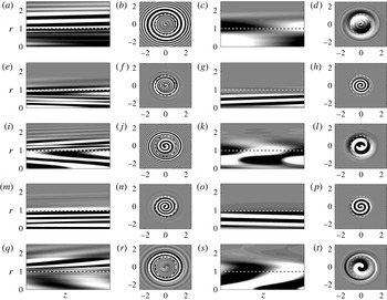
Figure 1. The fitted mean velocity profiles from Oberleithner et al. (Reference Oberleithner, Sieber, Nayeri, Paschereit, Petz, Hege, Noack and Wygnanski2011) in a meridian
 $(\unicode[STIX]{x1D703})$
plane, showing (a) axial profiles (
$(\unicode[STIX]{x1D703})$
plane, showing (a) axial profiles (
 $\bar{u}_{z}$
) and (b) azimuthal profiles (
$\bar{u}_{z}$
) and (b) azimuthal profiles (
 $\bar{u}_{\unicode[STIX]{x1D703}}$
) at selected streamwise locations where transient growths are computed in § 5.3. The shaded area approximately represents the streamwise extent of the recirculation bubble, while the dashed curves are for locations downstream of the bubble collapse and within the wake region.
$\bar{u}_{\unicode[STIX]{x1D703}}$
) at selected streamwise locations where transient growths are computed in § 5.3. The shaded area approximately represents the streamwise extent of the recirculation bubble, while the dashed curves are for locations downstream of the bubble collapse and within the wake region.
The distinguishing feature of this time-averaged swirling flow, as seen in figure 1, is the appearance of a region of reversed flow in the form of a bubble, immediately downstream of the nozzle, which is bound by the inner shear layer and the upstream and downstream stagnation points. This bubble collapses at approximately
 $z^{\ast }/D^{\ast }>1.4$
, as indicated in the figure, after which the jet enters a region resembling a wake with the gradual increase of axial centreline velocity, further downstream. The axial
$z^{\ast }/D^{\ast }>1.4$
, as indicated in the figure, after which the jet enters a region resembling a wake with the gradual increase of axial centreline velocity, further downstream. The axial
 $\bar{u}_{z}$
and azimuthal
$\bar{u}_{z}$
and azimuthal
 $\bar{u}_{\unicode[STIX]{x1D703}}$
profiles shown in figure 1 are analytical fits (due to Monkewitz & Sohn Reference Monkewitz and Sohn1988; Michalke Reference Michalke1999) to the actual measurements, whose details are in Oberleithner et al. (Reference Oberleithner, Sieber, Nayeri, Paschereit, Petz, Hege, Noack and Wygnanski2011), and are not repeated here. Note here that, in Oberleithner et al. (Reference Oberleithner, Sieber, Nayeri, Paschereit, Petz, Hege, Noack and Wygnanski2011), fitting parameters for the mean profile curves are available at only four streamwise locations of figure 1, while at other locations the same curve fitting procedure described in Oberleithner et al. (Reference Oberleithner, Sieber, Nayeri, Paschereit, Petz, Hege, Noack and Wygnanski2011) is used to obtain the corresponding parameter values. Similar to Gallaire et al. (Reference Gallaire, Ruith, Meiburg, Chomaz and Huerre2006), this time-averaged flow can be taken as a baseline axisymmetric breakdown state to study the effects of helical modes (
$\bar{u}_{\unicode[STIX]{x1D703}}$
profiles shown in figure 1 are analytical fits (due to Monkewitz & Sohn Reference Monkewitz and Sohn1988; Michalke Reference Michalke1999) to the actual measurements, whose details are in Oberleithner et al. (Reference Oberleithner, Sieber, Nayeri, Paschereit, Petz, Hege, Noack and Wygnanski2011), and are not repeated here. Note here that, in Oberleithner et al. (Reference Oberleithner, Sieber, Nayeri, Paschereit, Petz, Hege, Noack and Wygnanski2011), fitting parameters for the mean profile curves are available at only four streamwise locations of figure 1, while at other locations the same curve fitting procedure described in Oberleithner et al. (Reference Oberleithner, Sieber, Nayeri, Paschereit, Petz, Hege, Noack and Wygnanski2011) is used to obtain the corresponding parameter values. Similar to Gallaire et al. (Reference Gallaire, Ruith, Meiburg, Chomaz and Huerre2006), this time-averaged flow can be taken as a baseline axisymmetric breakdown state to study the effects of helical modes (
 $m>0$
) on its stability, which we do here by focusing on the non-modal linear dynamics, via a local analysis. In doing so, along with the neglect of
$m>0$
) on its stability, which we do here by focusing on the non-modal linear dynamics, via a local analysis. In doing so, along with the neglect of
 $\bar{u}_{r}$
, we invoke the parallel (or quasi-parallel) flow assumption for all the mean profiles. As discussed in § 1, flow parallelism is unlikely to be valid at
$\bar{u}_{r}$
, we invoke the parallel (or quasi-parallel) flow assumption for all the mean profiles. As discussed in § 1, flow parallelism is unlikely to be valid at
 $z^{\ast }/D^{\ast }=0.25$
which is at the upstream edge of the bubble and at locations
$z^{\ast }/D^{\ast }=0.25$
which is at the upstream edge of the bubble and at locations
 $z^{\ast }/D^{\ast }=1.5$
and 1.6 which are at its downstream edge, although we do report results from some of these locations too. On the contrary, positions in the wake from around
$z^{\ast }/D^{\ast }=1.5$
and 1.6 which are at its downstream edge, although we do report results from some of these locations too. On the contrary, positions in the wake from around
 $z^{\ast }/D^{\ast }\geqslant 1.8$
may yield more accurate local answers as might the location around
$z^{\ast }/D^{\ast }\geqslant 1.8$
may yield more accurate local answers as might the location around
 $z^{\ast }/D^{\ast }=1.0$
, located near the middle of the bubble.
$z^{\ast }/D^{\ast }=1.0$
, located near the middle of the bubble.
3 Methodology
3.1 Linear stability equations
The incompressible, viscous equations without body force terms are formulated in cylindrical polar coordinates (
 $r,\unicode[STIX]{x1D703},z$
), non-dimensionalized at each streamwise location by the local maxima of the mean streamwise velocity
$r,\unicode[STIX]{x1D703},z$
), non-dimensionalized at each streamwise location by the local maxima of the mean streamwise velocity
 $\bar{u}_{z}^{\ast }|_{max}$
and its corresponding radial location
$\bar{u}_{z}^{\ast }|_{max}$
and its corresponding radial location
 $r^{\ast }|_{max}$
(see figure 1) to yield
$r^{\ast }|_{max}$
(see figure 1) to yield
 $$\begin{eqnarray}\displaystyle & \displaystyle \frac{\unicode[STIX]{x2202}u_{r}}{\unicode[STIX]{x2202}r}+\frac{u_{r}}{r}+\frac{1}{r}\frac{\unicode[STIX]{x2202}u_{\unicode[STIX]{x1D703}}}{\unicode[STIX]{x2202}\unicode[STIX]{x1D703}}+\frac{\unicode[STIX]{x2202}u_{z}}{\unicode[STIX]{x2202}z}=0, & \displaystyle\end{eqnarray}$$
 $$\begin{eqnarray}\displaystyle & \displaystyle \frac{\text{D}u_{r}}{\text{D}t}-\frac{u_{\unicode[STIX]{x1D703}}^{2}}{r}=-\frac{1}{\unicode[STIX]{x1D70C}}\frac{\unicode[STIX]{x2202}p}{\unicode[STIX]{x2202}r}+\frac{1}{Re}\left(\unicode[STIX]{x0394}u_{r}-\frac{u_{r}}{r^{2}}-\frac{2}{r^{2}}\frac{\unicode[STIX]{x2202}u_{\unicode[STIX]{x1D703}}}{\unicode[STIX]{x2202}\unicode[STIX]{x1D703}}\right), & \displaystyle\end{eqnarray}$$
 $$\begin{eqnarray}\displaystyle & \displaystyle \frac{\text{D}u_{\unicode[STIX]{x1D703}}}{\text{D}t}+\frac{u_{r}u_{\unicode[STIX]{x1D703}}}{r}=-\frac{1}{\unicode[STIX]{x1D70C}r}\frac{\unicode[STIX]{x2202}p}{\unicode[STIX]{x2202}\unicode[STIX]{x1D703}}+\frac{1}{Re}\left(\unicode[STIX]{x0394}u_{\unicode[STIX]{x1D703}}-\frac{u_{\unicode[STIX]{x1D703}}}{r^{2}}+\frac{2}{r^{2}}\frac{\unicode[STIX]{x2202}u_{r}}{\unicode[STIX]{x2202}\unicode[STIX]{x1D703}}\right), & \displaystyle\end{eqnarray}$$
 $$\begin{eqnarray}\displaystyle & \displaystyle \frac{\text{D}u_{z}}{\text{D}t}=-\frac{1}{\unicode[STIX]{x1D70C}}\frac{\unicode[STIX]{x2202}p}{\unicode[STIX]{x2202}z}+\frac{1}{Re}\unicode[STIX]{x0394}u_{z}, & \displaystyle\end{eqnarray}$$
 $\text{D}/\text{D}t$
and
$\text{D}/\text{D}t$
and
 $\unicode[STIX]{x1D6E5}$
are respectively the material derivative and the Laplacian operator, given by
$\unicode[STIX]{x1D6E5}$
are respectively the material derivative and the Laplacian operator, given by  $$\begin{eqnarray}\displaystyle & \displaystyle \frac{\text{D}}{\text{D}t}=\frac{\unicode[STIX]{x2202}}{\unicode[STIX]{x2202}t}+u_{r}\frac{\unicode[STIX]{x2202}}{\unicode[STIX]{x2202}r}+\frac{u_{\unicode[STIX]{x1D703}}}{r}\frac{\unicode[STIX]{x2202}}{\unicode[STIX]{x2202}\unicode[STIX]{x1D703}}+u_{z}\frac{\unicode[STIX]{x2202}}{\unicode[STIX]{x2202}z}, & \displaystyle\end{eqnarray}$$
 $$\begin{eqnarray}\displaystyle & \displaystyle \unicode[STIX]{x1D6E5}=\frac{\unicode[STIX]{x2202}^{2}}{\unicode[STIX]{x2202}r^{2}}+\frac{1}{r}\frac{\unicode[STIX]{x2202}}{\unicode[STIX]{x2202}r}+\frac{1}{r^{2}}\frac{\unicode[STIX]{x2202}^{2}}{\unicode[STIX]{x2202}\unicode[STIX]{x1D703}^{2}}+\frac{\unicode[STIX]{x2202}^{2}}{\unicode[STIX]{x2202}z^{2}}, & \displaystyle\end{eqnarray}$$
 $Re=\bar{u}_{z}^{\ast }|_{max}r^{\ast }|_{max}/\unicode[STIX]{x1D708}$
being the local Reynolds number that varies along the streamwise direction (in contrast to
$Re=\bar{u}_{z}^{\ast }|_{max}r^{\ast }|_{max}/\unicode[STIX]{x1D708}$
being the local Reynolds number that varies along the streamwise direction (in contrast to
 $Re_{D}$
),
$Re_{D}$
),
 $\unicode[STIX]{x1D708}$
is the kinematic viscosity and
$\unicode[STIX]{x1D708}$
is the kinematic viscosity and
 $\unicode[STIX]{x1D70C}$
is the density.
$\unicode[STIX]{x1D70C}$
is the density. Linear stability equations are now formed from (3.1) via standard procedures where the flow variables
 $\boldsymbol{q}$
are first decomposed into mean
$\boldsymbol{q}$
are first decomposed into mean
 $\bar{\boldsymbol{q}}$
and fluctuations
$\bar{\boldsymbol{q}}$
and fluctuations
 $\boldsymbol{q}^{\prime }$
from which the mean equations are then subtracted out. The fluctuations are modelled to possess travelling-wave-like solutions along the axial
$\boldsymbol{q}^{\prime }$
from which the mean equations are then subtracted out. The fluctuations are modelled to possess travelling-wave-like solutions along the axial
 $z$
and azimuthal
$z$
and azimuthal
 $\unicode[STIX]{x1D703}$
directions with a periodic time
$\unicode[STIX]{x1D703}$
directions with a periodic time
 $t$
via
$t$
via
 $$\begin{eqnarray}\displaystyle \boldsymbol{q}^{\prime }(r,\unicode[STIX]{x1D703},z,t)=\hat{\boldsymbol{q}}(r)\exp (\text{i}\unicode[STIX]{x1D6FC}z+\text{i}m\unicode[STIX]{x1D703}-\text{i}\unicode[STIX]{x1D714}t), & & \displaystyle\end{eqnarray}$$
where
 $\boldsymbol{q}^{\prime }=[u_{r}^{\prime }~u_{\unicode[STIX]{x1D703}}^{\prime }~u_{z}^{\prime }~p^{\prime }]^{\text{T}}$
,
$\boldsymbol{q}^{\prime }=[u_{r}^{\prime }~u_{\unicode[STIX]{x1D703}}^{\prime }~u_{z}^{\prime }~p^{\prime }]^{\text{T}}$
,
 $\hat{\boldsymbol{q}}(r)$
is the unknown complex eigenfunction,
$\hat{\boldsymbol{q}}(r)$
is the unknown complex eigenfunction,
 $\unicode[STIX]{x1D6FC}$
and
$\unicode[STIX]{x1D6FC}$
and
 $m$
are respectively the axial and azimuthal wavenumbers and
$m$
are respectively the axial and azimuthal wavenumbers and
 $\unicode[STIX]{x1D714}$
is the frequency, a complex number in our temporal setting. On using (3.3) in (3.1) and linearizing for small fluctuations, the stability equations may be written as a generalized eigenvalue problem of the form
$\unicode[STIX]{x1D714}$
is the frequency, a complex number in our temporal setting. On using (3.3) in (3.1) and linearizing for small fluctuations, the stability equations may be written as a generalized eigenvalue problem of the form
 $$\begin{eqnarray}\displaystyle \unicode[STIX]{x1D63E}\boldsymbol{\cdot }\hat{\boldsymbol{q}}=\unicode[STIX]{x1D706}\;\hat{\boldsymbol{q}}, & & \displaystyle\end{eqnarray}$$
where
 $$\begin{eqnarray}\displaystyle \unicode[STIX]{x1D63E}=\unicode[STIX]{x1D63C}^{-1}\unicode[STIX]{x1D63D}\quad \text{and}\quad \unicode[STIX]{x1D706}=\text{i}/\unicode[STIX]{x1D714}, & & \displaystyle\end{eqnarray}$$
where,
 $\unicode[STIX]{x1D63C}$
and
$\unicode[STIX]{x1D63C}$
and
 $\unicode[STIX]{x1D63D}$
are
$\unicode[STIX]{x1D63D}$
are
 $4\times 4$
matrices (
$4\times 4$
matrices (
 $\unicode[STIX]{x1D63D}$
is singular) whose details are given in appendix B.
$\unicode[STIX]{x1D63D}$
is singular) whose details are given in appendix B.
3.2 Boundary conditions
At
 $r=0$
, the boundary conditions depend upon the azimuthal wavenumber
$r=0$
, the boundary conditions depend upon the azimuthal wavenumber
 $m$
, whose treatment is standard (see e.g. Batchelor & Gill Reference Batchelor and Gill1962; Khorrami, Malik & Ash Reference Khorrami, Malik and Ash1989; Yadav & Samanta Reference Yadav and Samanta2017):
$m$
, whose treatment is standard (see e.g. Batchelor & Gill Reference Batchelor and Gill1962; Khorrami, Malik & Ash Reference Khorrami, Malik and Ash1989; Yadav & Samanta Reference Yadav and Samanta2017):
 $$\begin{eqnarray}\left.\begin{array}{@{}cccc@{}}m=0:\hat{u} _{r}=0, & \hat{u} _{\unicode[STIX]{x1D703}}=0, & \hat{u} _{z}=\unicode[STIX]{x1D712}_{1}, & \hat{p}=\unicode[STIX]{x1D712}_{2},\\ m=1:\hat{u} _{r}+\text{i}\hat{u} _{\unicode[STIX]{x1D703}}=0, & \displaystyle {\displaystyle \frac{\unicode[STIX]{x2202}\hat{u} _{r}}{\unicode[STIX]{x2202}r}}+\text{i}{\displaystyle \frac{\unicode[STIX]{x2202}\hat{u} _{\unicode[STIX]{x1D703}}}{\unicode[STIX]{x2202}r}}=0, & \hat{u} _{z}=0, & \hat{p}=0,\\ m>1:\hat{u} _{r}=0, & \hat{u} _{\unicode[STIX]{x1D703}}=0, & \hat{u} _{z}=0, & \hat{p}=0,\end{array}\right\}\end{eqnarray}$$
while at
 $r=r_{max}$
, the maximum radial extent of the mean flow, all fluctuations go to zero:
$r=r_{max}$
, the maximum radial extent of the mean flow, all fluctuations go to zero:
 $$\begin{eqnarray}\forall m:\hat{u} _{r}=0,\quad \hat{u} _{\unicode[STIX]{x1D703}}=0,\quad \hat{u} _{z}=0,\quad \hat{p}=0,\end{eqnarray}$$
where
 $\unicode[STIX]{x1D712}_{1}$
and
$\unicode[STIX]{x1D712}_{1}$
and
 $\unicode[STIX]{x1D712}_{2}$
are constants, set here to zero, with no loss of accuracy.
$\unicode[STIX]{x1D712}_{2}$
are constants, set here to zero, with no loss of accuracy.
Equation (3.4) along with the boundary conditions (3.6) and (3.7) are solved using a standard Chebyshev spectral collocation technique, described in detail in Yadav & Samanta (Reference Yadav and Samanta2017). A simple linear mapping of
 $r=(1+\unicode[STIX]{x1D709})/2$
is used to map the Chebyshev interval
$r=(1+\unicode[STIX]{x1D709})/2$
is used to map the Chebyshev interval
 $-1\leqslant \unicode[STIX]{x1D709}\leqslant 1$
to the physical domain
$-1\leqslant \unicode[STIX]{x1D709}\leqslant 1$
to the physical domain
 $0\leqslant r\leqslant r_{max}$
. Note here that unlike in Oberleithner et al. (Reference Oberleithner, Sieber, Nayeri, Paschereit, Petz, Hege, Noack and Wygnanski2011), no stretching of collocation points toward the jet core is done, which is presumed to increase the convergence speed of exponentially varying modes in an eigen system. This is because faster convergence of the continuous spectrum is deemed equally important in this work. In fact, modes within the continuous spectrum, as discussed later, are known to dominate near and outside the jet outer shear layer that makes the natural Gauss–Lobatto-type clustering more efficient, apart from the fact that most types of numerical stretching are known to worsen the condition number of matrices, e.g. that of
$0\leqslant r\leqslant r_{max}$
. Note here that unlike in Oberleithner et al. (Reference Oberleithner, Sieber, Nayeri, Paschereit, Petz, Hege, Noack and Wygnanski2011), no stretching of collocation points toward the jet core is done, which is presumed to increase the convergence speed of exponentially varying modes in an eigen system. This is because faster convergence of the continuous spectrum is deemed equally important in this work. In fact, modes within the continuous spectrum, as discussed later, are known to dominate near and outside the jet outer shear layer that makes the natural Gauss–Lobatto-type clustering more efficient, apart from the fact that most types of numerical stretching are known to worsen the condition number of matrices, e.g. that of
 $\unicode[STIX]{x1D63C}$
in (3.5) (similar to in Mao & Sherwin Reference Mao and Sherwin2011).
$\unicode[STIX]{x1D63C}$
in (3.5) (similar to in Mao & Sherwin Reference Mao and Sherwin2011).
3.3 Local transient analysis
In this section, only a brief overview of the local transient analysis, as used in this work is given, which follows established procedures (see e.g. Schmid & Henningson Reference Schmid and Henningson2001, for more details). In this, once we assume solutions of the form
 $\tilde{\boldsymbol{q}}(r,t)=\hat{\boldsymbol{q}}(r)\exp (-\text{i}\unicode[STIX]{x1D714}t)$
, the corresponding initial value problem for (3.4) is
$\tilde{\boldsymbol{q}}(r,t)=\hat{\boldsymbol{q}}(r)\exp (-\text{i}\unicode[STIX]{x1D714}t)$
, the corresponding initial value problem for (3.4) is
 $$\begin{eqnarray}\displaystyle \unicode[STIX]{x1D63D}\boldsymbol{\cdot }\frac{\unicode[STIX]{x2202}\tilde{\boldsymbol{q}}}{\unicode[STIX]{x2202}t}=\unicode[STIX]{x1D63C}\boldsymbol{\cdot }\tilde{\boldsymbol{q}}, & & \displaystyle\end{eqnarray}$$
where on restricting to the first
 $M$
eigenfunctions of
$M$
eigenfunctions of
 $\unicode[STIX]{x1D63E}$
, a new vector
$\unicode[STIX]{x1D63E}$
, a new vector
 $\unicode[STIX]{x1D73F}$
may be introduced (see Schmid & Henningson Reference Schmid and Henningson2001) via
$\unicode[STIX]{x1D73F}$
may be introduced (see Schmid & Henningson Reference Schmid and Henningson2001) via
 $$\begin{eqnarray}\displaystyle \tilde{\boldsymbol{q}}(r,t)=\mathop{\sum }_{j=1}^{M}\unicode[STIX]{x1D705}_{j}(t)\hat{\boldsymbol{q}}_{j}(r), & & \displaystyle\end{eqnarray}$$
where
 $\unicode[STIX]{x1D705}_{j}(t)=\exp (-\text{i}\unicode[STIX]{x1D714}_{j}t)\unicode[STIX]{x1D705}_{j}(0)$
are the expansion coefficients for the reduced basis of eigenfunctions
$\unicode[STIX]{x1D705}_{j}(t)=\exp (-\text{i}\unicode[STIX]{x1D714}_{j}t)\unicode[STIX]{x1D705}_{j}(0)$
are the expansion coefficients for the reduced basis of eigenfunctions
 $\{\hat{\boldsymbol{q}}_{1},\ldots ,\hat{\boldsymbol{q}}_{M}\}$
of (3.4), with
$\{\hat{\boldsymbol{q}}_{1},\ldots ,\hat{\boldsymbol{q}}_{M}\}$
of (3.4), with
 $\unicode[STIX]{x1D714}_{j}$
being the corresponding eigenvalues. In this work,
$\unicode[STIX]{x1D714}_{j}$
being the corresponding eigenvalues. In this work,
 $M$
contains all the stable eigenmodes contained within
$M$
contains all the stable eigenmodes contained within
 $\unicode[STIX]{x1D714}_{j}>-5$
, yielding sufficiently accurate transient growth for all the cases considered. Now, the energy norm
$\unicode[STIX]{x1D714}_{j}>-5$
, yielding sufficiently accurate transient growth for all the cases considered. Now, the energy norm
 $\Vert \tilde{\boldsymbol{q}}\Vert _{E}^{2}$
using (3.9) yields
$\Vert \tilde{\boldsymbol{q}}\Vert _{E}^{2}$
using (3.9) yields
 $$\begin{eqnarray}\displaystyle \Vert \tilde{\boldsymbol{q}}\Vert _{E}^{2}=\frac{\unicode[STIX]{x03C0}}{2}\unicode[STIX]{x1D73F}^{H}\unicode[STIX]{x1D650}\unicode[STIX]{x1D73F}=\frac{\unicode[STIX]{x03C0}}{2}\unicode[STIX]{x1D73F}^{H}\unicode[STIX]{x1D641}^{H}\unicode[STIX]{x1D641}\unicode[STIX]{x1D73F}=\Vert \unicode[STIX]{x1D641}\unicode[STIX]{x1D73F}\Vert _{2}^{2}, & & \displaystyle\end{eqnarray}$$
where
 $(\,)_{2}$
denotes the matrix 2-norm (Euclidean or the
$(\,)_{2}$
denotes the matrix 2-norm (Euclidean or the
 $\unicode[STIX]{x1D647}^{2}$
norm),
$\unicode[STIX]{x1D647}^{2}$
norm),
 $(\,)^{H}$
indicates conjugate transpose,
$(\,)^{H}$
indicates conjugate transpose,
 $\unicode[STIX]{x1D650}=\unicode[STIX]{x1D641}^{H}\unicode[STIX]{x1D641}$
is a square Hermitian and positive definite matrix of dimension
$\unicode[STIX]{x1D650}=\unicode[STIX]{x1D641}^{H}\unicode[STIX]{x1D641}$
is a square Hermitian and positive definite matrix of dimension
 $M$
, whose elements are obtained via the Chebyshev coefficients (see also Reddy, Schmid & Henningson Reference Reddy, Schmid and Henningson1993) to yield
$M$
, whose elements are obtained via the Chebyshev coefficients (see also Reddy, Schmid & Henningson Reference Reddy, Schmid and Henningson1993) to yield
 $$\begin{eqnarray}\displaystyle U_{ij}=\hat{\boldsymbol{q}}_{i}^{H}\unicode[STIX]{x1D6E4}_{1}\hat{\boldsymbol{q}}_{j}+\hat{\boldsymbol{q}}_{i}^{H}\unicode[STIX]{x1D6E4}_{2}\hat{\boldsymbol{q}}_{j}, & & \displaystyle\end{eqnarray}$$
where
 $$\begin{eqnarray}\unicode[STIX]{x1D6E4}_{1}=\int _{-1}^{1}T_{i}(\unicode[STIX]{x1D709})T_{j}(\unicode[STIX]{x1D709})\,\text{d}\unicode[STIX]{x1D709}=\left\{\begin{array}{@{}ll@{}}0,\quad & \text{if}~i+j~\text{is odd},\\ {\displaystyle \frac{1}{1-(i+j)^{2}}}+{\displaystyle \frac{1}{1-(i-j)^{2}}},\quad & \text{if}~i+j~\text{is even},\end{array}\right.\end{eqnarray}$$
and
 $$\begin{eqnarray}\unicode[STIX]{x1D6E4}_{2}=\int _{-1}^{1}T_{i}(\unicode[STIX]{x1D709})T_{j}(\unicode[STIX]{x1D709})\unicode[STIX]{x1D709}\,\text{d}\unicode[STIX]{x1D709}=\left\{\begin{array}{@{}ll@{}}{\displaystyle \frac{1}{4-(i+j)^{2}}}+{\displaystyle \frac{1}{4-(i-j)^{2}}},\quad & \text{if}~i+j~\text{is odd},\\ 0,\quad & \text{if}~i+j~\text{is even},\end{array}\right.\end{eqnarray}$$
where
 $T_{i}$
is the
$T_{i}$
is the
 $i$
th Chebyshev polynomial.
$i$
th Chebyshev polynomial.

Figure 2. Convergence of the spectrum (symbols) and
 $\unicode[STIX]{x1D716}$
-pseudospectrum (lines) for the swirling mean flow of figure 1 at
$\unicode[STIX]{x1D716}$
-pseudospectrum (lines) for the swirling mean flow of figure 1 at
 $m=1$
,
$m=1$
,
 $\unicode[STIX]{x1D6FC}=1$
and
$\unicode[STIX]{x1D6FC}=1$
and
 $z^{\ast }/D^{\ast }=0.25$
. In (a) the radial extent of the domain (
$z^{\ast }/D^{\ast }=0.25$
. In (a) the radial extent of the domain (
 $r_{max}$
) varies, where (▵, – – –)
$r_{max}$
) varies, where (▵, – – –)
 $r_{max}=5$
; (○, ——)
$r_{max}=5$
; (○, ——)
 $r_{max}=10$
; and (▿, –
$r_{max}=10$
; and (▿, –
 $\cdot$
–
$\cdot$
–
 $\cdot$
)
$\cdot$
)
 $r_{max}=20$
, with
$r_{max}=20$
, with
 $N=1000$
except the last case where
$N=1000$
except the last case where
 $N=1500$
. In (b) the Chebyshev polynomial order (
$N=1500$
. In (b) the Chebyshev polynomial order (
 $N$
) varies, where (▵, – – –)
$N$
) varies, where (▵, – – –)
 $N=800$
; (▫, –
$N=800$
; (▫, –
 $\cdot$
–
$\cdot$
–
 $\cdot$
)
$\cdot$
)
 $N=900$
; (○, ——)
$N=900$
; (○, ——)
 $N=1000$
; and (▿,
$N=1000$
; and (▿,
 $\cdots \cdots$
)
$\cdots \cdots$
)
 $N=1100$
, with
$N=1100$
, with
 $r_{max}=10$
in all cases. The
$r_{max}=10$
in all cases. The
 $\unicode[STIX]{x1D716}$
-pseudospectrum contours in all cases indicate
$\unicode[STIX]{x1D716}$
-pseudospectrum contours in all cases indicate
 $\unicode[STIX]{x1D716}=10^{-9}$
.
$\unicode[STIX]{x1D716}=10^{-9}$
.
The maximum amplification
 $G(\unicode[STIX]{x1D70F})$
at time
$G(\unicode[STIX]{x1D70F})$
at time
 $\unicode[STIX]{x1D70F}$
, over all possible initial conditions (see Mao & Sherwin Reference Mao and Sherwin2012), on using (3.10) yields
$\unicode[STIX]{x1D70F}$
, over all possible initial conditions (see Mao & Sherwin Reference Mao and Sherwin2012), on using (3.10) yields
 $$\begin{eqnarray}\displaystyle G(\unicode[STIX]{x1D70F})=\sup _{\tilde{\boldsymbol{q}}_{0}}\frac{\Vert \tilde{\boldsymbol{q}}_{\unicode[STIX]{x1D70F}}\Vert _{E}^{2}}{\Vert \tilde{\boldsymbol{q}}_{0}\Vert _{E}^{2}}=\Vert \unicode[STIX]{x1D641}\exp (-\text{i}\unicode[STIX]{x1D734}\unicode[STIX]{x1D70F})\unicode[STIX]{x1D641}^{-1}\Vert _{2}^{2}, & & \displaystyle\end{eqnarray}$$
where
 $\exp (-\text{i}\unicode[STIX]{x1D734}\unicode[STIX]{x1D70F})$
is a diagonal matrix whose elements are
$\exp (-\text{i}\unicode[STIX]{x1D734}\unicode[STIX]{x1D70F})$
is a diagonal matrix whose elements are
 $\exp (-\text{i}\unicode[STIX]{x1D714}_{j}\unicode[STIX]{x1D70F})$
for
$\exp (-\text{i}\unicode[STIX]{x1D714}_{j}\unicode[STIX]{x1D70F})$
for
 $j=1$
to
$j=1$
to
 $M$
,
$M$
,
 $\tilde{\boldsymbol{q}}_{0}$
is the optimal initial perturbation while
$\tilde{\boldsymbol{q}}_{0}$
is the optimal initial perturbation while
 $\tilde{\boldsymbol{q}}_{\unicode[STIX]{x1D70F}}$
is the corresponding outcome at time
$\tilde{\boldsymbol{q}}_{\unicode[STIX]{x1D70F}}$
is the corresponding outcome at time
 $\unicode[STIX]{x1D70F}$
. We note here that the 2-norm of a matrix is simply its principal singular value, denoted here by
$\unicode[STIX]{x1D70F}$
. We note here that the 2-norm of a matrix is simply its principal singular value, denoted here by
 $\unicode[STIX]{x1D70E}_{1}(\,)$
, and thus the transient gain of (3.14) is
$\unicode[STIX]{x1D70E}_{1}(\,)$
, and thus the transient gain of (3.14) is
 $$\begin{eqnarray}\displaystyle G(\unicode[STIX]{x1D70F})=\unicode[STIX]{x1D70E}_{1}^{2}(\unicode[STIX]{x1D641}\exp (-\text{i}\unicode[STIX]{x1D734}\unicode[STIX]{x1D70F})\unicode[STIX]{x1D641}^{-1}), & & \displaystyle\end{eqnarray}$$
which can thus be computed by simply knowing the eigenvalues
 $\unicode[STIX]{x1D714}_{j}$
and the vector eigenfunctions
$\unicode[STIX]{x1D714}_{j}$
and the vector eigenfunctions
 $\hat{\boldsymbol{q}}_{j}$
of the generalized eigenvalue problem (3.4).
$\hat{\boldsymbol{q}}_{j}$
of the generalized eigenvalue problem (3.4).
Finally, the optimal initial perturbation and its outcome can be obtained via the use of singular value decomposition principles, requiring (see e.g. Schmid & Henningson Reference Schmid and Henningson2001)
 $$\begin{eqnarray}\displaystyle \unicode[STIX]{x1D641}\exp (-\text{i}\unicode[STIX]{x1D734}\unicode[STIX]{x1D70F})\unicode[STIX]{x1D641}^{-1}\boldsymbol{v}_{1}=\boldsymbol{u}_{1}\unicode[STIX]{x1D70E}_{1}, & & \displaystyle\end{eqnarray}$$
which describes a mapping
 $\unicode[STIX]{x1D641}\exp (-\text{i}\unicode[STIX]{x1D734}\unicode[STIX]{x1D70F})\unicode[STIX]{x1D641}^{-1}$
of the input vector
$\unicode[STIX]{x1D641}\exp (-\text{i}\unicode[STIX]{x1D734}\unicode[STIX]{x1D70F})\unicode[STIX]{x1D641}^{-1}$
of the input vector
 $\boldsymbol{v}_{1}$
(right singular vector) onto the output vector
$\boldsymbol{v}_{1}$
(right singular vector) onto the output vector
 $\boldsymbol{u}_{1}$
(left singular vector), amplified by
$\boldsymbol{u}_{1}$
(left singular vector), amplified by
 $\unicode[STIX]{x1D70E}_{1}$
, the 2-norm of this mapping, at time
$\unicode[STIX]{x1D70E}_{1}$
, the 2-norm of this mapping, at time
 $\unicode[STIX]{x1D70F}$
. These optimal conditions corresponding to
$\unicode[STIX]{x1D70F}$
. These optimal conditions corresponding to
 $G(\unicode[STIX]{x1D70F})$
of (3.15) are simply
$G(\unicode[STIX]{x1D70F})$
of (3.15) are simply
 $$\begin{eqnarray}\displaystyle \tilde{\boldsymbol{q}}_{0}=\unicode[STIX]{x1D64C}\unicode[STIX]{x1D641}^{-1}\boldsymbol{v}_{1}\quad \text{and}\quad \tilde{\boldsymbol{q}}_{\unicode[STIX]{x1D70F}}=\unicode[STIX]{x1D64C}\unicode[STIX]{x1D641}^{-1}\boldsymbol{u}_{1}, & & \displaystyle\end{eqnarray}$$
where
 $\unicode[STIX]{x1D64C}$
is a matrix of eigenvectors obtained from (3.4) (see also Mao & Sherwin Reference Mao and Sherwin2012).
$\unicode[STIX]{x1D64C}$
is a matrix of eigenvectors obtained from (3.4) (see also Mao & Sherwin Reference Mao and Sherwin2012).
4 Spectrum and pseudospectrum
4.1 Discrete and continuous spectrum
Figure 2 shows the numerical convergence results of the discrete spectrum with respect to the radial extent of the domain
 $r_{max}$
(figure 2
a) and the order of Chebyshev polynomial
$r_{max}$
(figure 2
a) and the order of Chebyshev polynomial
 $N$
(figure 2
b). For the parametric space of figure 2, there are two discrete unstable modes (
$N$
(figure 2
b). For the parametric space of figure 2, there are two discrete unstable modes (
 $\unicode[STIX]{x1D714}_{i}>0$
) with exponential growth, which quickly converge to fixed points in the complex-
$\unicode[STIX]{x1D714}_{i}>0$
) with exponential growth, which quickly converge to fixed points in the complex-
 $\unicode[STIX]{x1D714}$
plane once the numerical tuning parameters of
$\unicode[STIX]{x1D714}$
plane once the numerical tuning parameters of
 $r_{max}$
and
$r_{max}$
and
 $N$
are gradually increased. Note that the order of Chebyshev polynomials required here for such a convergence is larger than in Oberleithner et al. (Reference Oberleithner, Sieber, Nayeri, Paschereit, Petz, Hege, Noack and Wygnanski2011), who reported convergence around
$N$
are gradually increased. Note that the order of Chebyshev polynomials required here for such a convergence is larger than in Oberleithner et al. (Reference Oberleithner, Sieber, Nayeri, Paschereit, Petz, Hege, Noack and Wygnanski2011), who reported convergence around
 $N=300$
. This is not surprising since we do not use any additional stretching of the Gauss–Lobatto points, as discussed before in § 3.2, since it can potentially worsen the convergence of the continuous spectrum. Once any of the discrete modes cross the neutral axis (
$N=300$
. This is not surprising since we do not use any additional stretching of the Gauss–Lobatto points, as discussed before in § 3.2, since it can potentially worsen the convergence of the continuous spectrum. Once any of the discrete modes cross the neutral axis (
 $\unicode[STIX]{x1D714}_{i}=0$
) toward the positive half-plane, they turn hydrodynamically unstable. The other discrete modes which are below this axis (
$\unicode[STIX]{x1D714}_{i}=0$
) toward the positive half-plane, they turn hydrodynamically unstable. The other discrete modes which are below this axis (
 $\unicode[STIX]{x1D714}_{i}<0$
) are stable modes with exponentially decaying eigenfunctions along the radial direction. Here, such stable exponential modes are seen to converge into branches of distinct shape, similar to e.g. the plane Couette and pipe flow spectra (see e.g. Schmid & Henningson Reference Schmid and Henningson2001).
$\unicode[STIX]{x1D714}_{i}<0$
) are stable modes with exponentially decaying eigenfunctions along the radial direction. Here, such stable exponential modes are seen to converge into branches of distinct shape, similar to e.g. the plane Couette and pipe flow spectra (see e.g. Schmid & Henningson Reference Schmid and Henningson2001).
The remaining spectrum is now referred to as the continuous spectrum, where we introduce classifications originally due to Obrist & Schmid (Reference Obrist and Schmid2010), Mao & Sherwin (Reference Mao and Sherwin2011). Within this spectrum, we classify as ‘potential modes’ those that have significant radial variations outside the jet core, while still being asymptotically stable, with a slower algebraic decay (rather than the exponential decay of typical stable discrete modes) at larger radial distances (see figure 3 for visualizations). In figure 2, these modes can be seen to be scattered over a large part of the spectrum, as their numbers depend upon
 $N$
. Mathematically, such modes are also known to be highly non-orthogonal (Obrist & Schmid Reference Obrist and Schmid2003; Mao & Sherwin Reference Mao and Sherwin2011) and hence there is a greater chance for them to participate in the short time transient growth, which we investigate here. Although seemingly spurious in nature, we shall find in § 4.2 that these potential modes too can be bounded (i.e. numerically converged) within an area in the complex plane via computing a pseudospectrum. Further, potential modes, for which
$N$
. Mathematically, such modes are also known to be highly non-orthogonal (Obrist & Schmid Reference Obrist and Schmid2003; Mao & Sherwin Reference Mao and Sherwin2011) and hence there is a greater chance for them to participate in the short time transient growth, which we investigate here. Although seemingly spurious in nature, we shall find in § 4.2 that these potential modes too can be bounded (i.e. numerically converged) within an area in the complex plane via computing a pseudospectrum. Further, potential modes, for which
 $\unicode[STIX]{x1D714}_{i}\rightarrow 0$
are called ‘free-stream modes’, following terminologies from boundary layer flows (see e.g. Mack Reference Mack1976; Zaki & Saha Reference Zaki and Saha2009), used for vortical flows by Mao & Sherwin (Reference Mao and Sherwin2011, Reference Mao and Sherwin2012), which at the limit have zero radial decay rate. As we shall see, these modes ensure a small but finite transient growth even at larger times. In this work,
$\unicode[STIX]{x1D714}_{i}\rightarrow 0$
are called ‘free-stream modes’, following terminologies from boundary layer flows (see e.g. Mack Reference Mack1976; Zaki & Saha Reference Zaki and Saha2009), used for vortical flows by Mao & Sherwin (Reference Mao and Sherwin2011, Reference Mao and Sherwin2012), which at the limit have zero radial decay rate. As we shall see, these modes ensure a small but finite transient growth even at larger times. In this work,
 $r_{max}=10$
and
$r_{max}=10$
and
 $N=1000$
are used in all computations.
$N=1000$
are used in all computations.

Figure 3. Radial decay of the potential mode (○) eigenfunctions
 $(|\hat{u} _{\unicode[STIX]{x1D703}}|)$
, shown in (b) for the modes highlighted in (a) at ●,
$(|\hat{u} _{\unicode[STIX]{x1D703}}|)$
, shown in (b) for the modes highlighted in (a) at ●,
 $(1.479-0.198\text{i})$
and ▪,
$(1.479-0.198\text{i})$
and ▪,
 $(1.436-0.348\text{i})$
in the marked group A region and at ●,
$(1.436-0.348\text{i})$
in the marked group A region and at ●,
 $(1.413-0.430\text{i})$
; ▪,
$(1.413-0.430\text{i})$
; ▪,
 $(1.384-0.516\text{i})$
and ♦,
$(1.384-0.516\text{i})$
and ♦,
 $(1.352-0.605\text{i})$
in the group B region. The parameters are
$(1.352-0.605\text{i})$
in the group B region. The parameters are
 $m=1$
,
$m=1$
,
 $\unicode[STIX]{x1D6FC}=1$
at
$\unicode[STIX]{x1D6FC}=1$
at
 $z^{\ast }/D^{\ast }=1.0$
, while in (a) the solid lines indicate the pseudospectrum of
$z^{\ast }/D^{\ast }=1.0$
, while in (a) the solid lines indicate the pseudospectrum of
 $\unicode[STIX]{x1D716}=10^{-6}$
; ♢ are discrete unstable and ▫ are discrete stable modes.
$\unicode[STIX]{x1D716}=10^{-6}$
; ♢ are discrete unstable and ▫ are discrete stable modes.
4.2 Pseudospectrum
The continuous modes which do not converge to fixed points in space may at first glance seem spurious. But on closer inspection, most of these modes in figure 2 are seen to roughly fill a rectangular area bounded approximately by the lines
 $\unicode[STIX]{x1D714}_{r}-1=0$
,
$\unicode[STIX]{x1D714}_{r}-1=0$
,
 $2\unicode[STIX]{x1D714}_{i}+\unicode[STIX]{x1D714}_{r}+1=0$
and the imaginary axis on its three sides, even as the numerical parameters are varied. These bounds do not appear to satisfy simple analytical relations, as they change significantly with the mean swirling flow developing downstream into the wake region.
$2\unicode[STIX]{x1D714}_{i}+\unicode[STIX]{x1D714}_{r}+1=0$
and the imaginary axis on its three sides, even as the numerical parameters are varied. These bounds do not appear to satisfy simple analytical relations, as they change significantly with the mean swirling flow developing downstream into the wake region.
Mathematically, the potential modes are not exact solutions of the modal system (3.4) and the corresponding boundary conditions, but satisfy them to some finite error. The
 $\unicode[STIX]{x1D716}$
-pseudospectrum
$\unicode[STIX]{x1D716}$
-pseudospectrum
 $\unicode[STIX]{x1D70E}_{\unicode[STIX]{x1D716}}$
of operator
$\unicode[STIX]{x1D70E}_{\unicode[STIX]{x1D716}}$
of operator
 $\unicode[STIX]{x1D63E}$
in (3.4) is required to quantify such errors in estimating the continuous modes, defined as (e.g. Trefethen & Embree Reference Trefethen and Embree2005)
$\unicode[STIX]{x1D63E}$
in (3.4) is required to quantify such errors in estimating the continuous modes, defined as (e.g. Trefethen & Embree Reference Trefethen and Embree2005)
 $$\begin{eqnarray}\displaystyle \unicode[STIX]{x1D70E}_{\unicode[STIX]{x1D716}}(\unicode[STIX]{x1D63E})=\{\unicode[STIX]{x1D706}\in \mathbb{C}:\Vert (\unicode[STIX]{x1D706}\unicode[STIX]{x1D644}-\unicode[STIX]{x1D63E})^{-1}\Vert _{2}<\unicode[STIX]{x1D716}\}, & & \displaystyle\end{eqnarray}$$
where
 $\unicode[STIX]{x1D706}$
is a complex eigenvalue and for
$\unicode[STIX]{x1D706}$
is a complex eigenvalue and for
 $\unicode[STIX]{x1D70E}_{\unicode[STIX]{x1D716}}$
the minimum singular value is used. For the discrete modes,
$\unicode[STIX]{x1D70E}_{\unicode[STIX]{x1D716}}$
the minimum singular value is used. For the discrete modes,
 $\unicode[STIX]{x1D716}=0$
, while for the continuous modes the finite magnitude of
$\unicode[STIX]{x1D716}=0$
, while for the continuous modes the finite magnitude of
 $\unicode[STIX]{x1D716}$
represents the error in estimating such modes.
$\unicode[STIX]{x1D716}$
represents the error in estimating such modes.
In this work, the
 $\unicode[STIX]{x1D716}$
-pseudospectrum is computed after projection of (3.4) into a lower-dimensional subspace via a partial Schur decomposition and then an inverse Lanczos iteration is done to compute the smallest singular values, following procedures described in Trefethen (Reference Trefethen1999).
$\unicode[STIX]{x1D716}$
-pseudospectrum is computed after projection of (3.4) into a lower-dimensional subspace via a partial Schur decomposition and then an inverse Lanczos iteration is done to compute the smallest singular values, following procedures described in Trefethen (Reference Trefethen1999).
Figure 2 also shows convergence of this
 $\unicode[STIX]{x1D716}$
-pseudospectrum where the
$\unicode[STIX]{x1D716}$
-pseudospectrum where the
 $\unicode[STIX]{x1D716}=10^{-9}$
contour is plotted for different parametric combinations of
$\unicode[STIX]{x1D716}=10^{-9}$
contour is plotted for different parametric combinations of
 $N$
and
$N$
and
 $r_{max}$
. In spite of an apparent lack of convergence of potential modes in the discrete sense, the
$r_{max}$
. In spite of an apparent lack of convergence of potential modes in the discrete sense, the
 $\unicode[STIX]{x1D716}$
-pseudospectrum contour clearly marks a region for such modes, whose top and right boundaries have converged for all parameters of the figure. This process also identifies a second distinct region for the potential modes at the junction of discrete stable mode branches, which are further classified in figure 3(a) for a different set of parameters. Such a splitting up of the potential modes region into two distinct sections is observed for the first time, which we label here as ‘group A’ and ‘group B’, respectively (see figure 3
a), where the former group lies at the junction of discrete stable mode branches. In figure 3(b), the absolute value of
$\unicode[STIX]{x1D716}$
-pseudospectrum contour clearly marks a region for such modes, whose top and right boundaries have converged for all parameters of the figure. This process also identifies a second distinct region for the potential modes at the junction of discrete stable mode branches, which are further classified in figure 3(a) for a different set of parameters. Such a splitting up of the potential modes region into two distinct sections is observed for the first time, which we label here as ‘group A’ and ‘group B’, respectively (see figure 3
a), where the former group lies at the junction of discrete stable mode branches. In figure 3(b), the absolute value of
 $\hat{u} _{\unicode[STIX]{x1D703}}$
is plotted for a selection of the potential modes, as marked in figure 3(a), gradually moving from the group A to group B regions. The nature of radial decay for all these modes in these twin regions follows
$\hat{u} _{\unicode[STIX]{x1D703}}$
is plotted for a selection of the potential modes, as marked in figure 3(a), gradually moving from the group A to group B regions. The nature of radial decay for all these modes in these twin regions follows
 $|\hat{u} _{\unicode[STIX]{x1D703}}|\sim r^{-\unicode[STIX]{x1D708}}$
(see e.g. Obrist & Schmid Reference Obrist and Schmid2010), where the exponent
$|\hat{u} _{\unicode[STIX]{x1D703}}|\sim r^{-\unicode[STIX]{x1D708}}$
(see e.g. Obrist & Schmid Reference Obrist and Schmid2010), where the exponent
 $\unicode[STIX]{x1D708}$
varies. The potential modes inside the group A region show characteristics resembling the discrete stable modes, with the first mode at
$\unicode[STIX]{x1D708}$
varies. The potential modes inside the group A region show characteristics resembling the discrete stable modes, with the first mode at
 $(1.479-0.198\text{i})$
in figure 3(a) being almost indistinguishable from a discrete stable mode with a peak near
$(1.479-0.198\text{i})$
in figure 3(a) being almost indistinguishable from a discrete stable mode with a peak near
 $r=0.5$
, as shown in figure 3(b). As we move toward the group B potential modes, a secondary peak appears outside the core vortical region, which becomes dominant for modes of the group B region, starting from the
$r=0.5$
, as shown in figure 3(b). As we move toward the group B potential modes, a secondary peak appears outside the core vortical region, which becomes dominant for modes of the group B region, starting from the
 $(1.413-0.430\text{i})$
mode marked in figure 3(a), with the eventual disappearance of the peak inside the jet core (see figure 3
b). The group A potential modes show slower decay at
$(1.413-0.430\text{i})$
mode marked in figure 3(a), with the eventual disappearance of the peak inside the jet core (see figure 3
b). The group A potential modes show slower decay at
 $\unicode[STIX]{x1D708}\approx 0.1$
, while for the group B modes this is much faster at
$\unicode[STIX]{x1D708}\approx 0.1$
, while for the group B modes this is much faster at
 $\unicode[STIX]{x1D708}\approx 0.4$
. As we shall find out in § 5.2, such different decay rates play an important role in their respective transient gain calculations, where the group A modes show higher dominance.
$\unicode[STIX]{x1D708}\approx 0.4$
. As we shall find out in § 5.2, such different decay rates play an important role in their respective transient gain calculations, where the group A modes show higher dominance.
The
 $\unicode[STIX]{x1D716}$
-pseudospectrum contours when plotted for the discrete modes appear as concentric circles (not shown here, but see e.g. Mao & Sherwin Reference Mao and Sherwin2011), which are possible to be resolved only at lower
$\unicode[STIX]{x1D716}$
-pseudospectrum contours when plotted for the discrete modes appear as concentric circles (not shown here, but see e.g. Mao & Sherwin Reference Mao and Sherwin2011), which are possible to be resolved only at lower
 $N$
, when some of these discrete modes are yet to be fully converged and thus have finite convergence errors.
$N$
, when some of these discrete modes are yet to be fully converged and thus have finite convergence errors.
The
 $\unicode[STIX]{x1D716}$
-pseudospectrum calculations as shown here, allow for a more definitive way of classifying the continuous spectrum discussed in § 4.1. We use this in the transient growth calculations of § 5, where we adopt the convention that potential modes belong to the part of the continuous spectrum bounded by a specific pseudospectrum contour level, chosen to be
$\unicode[STIX]{x1D716}$
-pseudospectrum calculations as shown here, allow for a more definitive way of classifying the continuous spectrum discussed in § 4.1. We use this in the transient growth calculations of § 5, where we adopt the convention that potential modes belong to the part of the continuous spectrum bounded by a specific pseudospectrum contour level, chosen to be
 $\unicode[STIX]{x1D716}=10^{-6}$
in this work (see also figure 4), with the remaining spectrum automatically classified into free-stream modes.
$\unicode[STIX]{x1D716}=10^{-6}$
in this work (see also figure 4), with the remaining spectrum automatically classified into free-stream modes.

Figure 4. Modal classification and local transient growths for (a,b)
 $m=1$
,
$m=1$
,
 $\unicode[STIX]{x1D6FC}=1$
at
$\unicode[STIX]{x1D6FC}=1$
at
 $z^{\ast }/D^{\ast }=0.25$
; (c,d)
$z^{\ast }/D^{\ast }=0.25$
; (c,d)
 $m=1$
,
$m=1$
,
 $\unicode[STIX]{x1D6FC}=1$
at
$\unicode[STIX]{x1D6FC}=1$
at
 $z^{\ast }/D^{\ast }=1.0$
and (e,f)
$z^{\ast }/D^{\ast }=1.0$
and (e,f)
 $m=2$
,
$m=2$
,
 $\unicode[STIX]{x1D6FC}=0.5$
at
$\unicode[STIX]{x1D6FC}=0.5$
at
 $z^{\ast }/D^{\ast }=2.6$
. The specific modes are ♦ discrete unstable; ▫ discrete stable; ○ potential and ▵ free-stream types, while the solid line in (a,c,e) show pseudospectrum of
$z^{\ast }/D^{\ast }=2.6$
. The specific modes are ♦ discrete unstable; ▫ discrete stable; ○ potential and ▵ free-stream types, while the solid line in (a,c,e) show pseudospectrum of
 $\unicode[STIX]{x1D716}=10^{-6}$
. Transient gains in (b,d,f) are from – – – discrete stable; –
$\unicode[STIX]{x1D716}=10^{-6}$
. Transient gains in (b,d,f) are from – – – discrete stable; –
 $\cdot$
–
$\cdot$
–
 $\cdot$
potential; –
$\cdot$
potential; –
 $\cdot \cdot$
–
$\cdot \cdot$
–
 $\cdot \cdot$
potential
$\cdot \cdot$
potential
 $+$
discrete stable; — — — all stable (including free stream) and —— all unstable modes, while the thick grey line indicates net gain from all modes. In addition, in (d) gain curves for –
$+$
discrete stable; — — — all stable (including free stream) and —— all unstable modes, while the thick grey line indicates net gain from all modes. In addition, in (d) gain curves for –
 $\cdot$
– ● – group A potential; –
$\cdot$
– ● – group A potential; –
 $\cdot$
– ▪ – group B potential and –
$\cdot$
– ▪ – group B potential and –
 $\cdot \cdot$
– ● – group A potential
$\cdot \cdot$
– ● – group A potential
 $+$
stable discrete modes are shown, where these potential mode groupings are labelled in (c). The insets in (a,c) show content of respective grey boxes.
$+$
stable discrete modes are shown, where these potential mode groupings are labelled in (c). The insets in (a,c) show content of respective grey boxes.
5 Results and discussion
In this section, our first goal is to establish the presence of strong transient growths in the swirling jet considered here and understand the relevance of this when compared to exponential modal growths from the discrete unstable mode(s). We quantify this growth by analysing a range of streamwise and azimuthal wavenumber perturbations on top of the mean profiles at the several streamwise locations shown in figure 1. Afterwards, our focus shifts to mechanisms where the aim is to find connections between known transient growth mechanisms with the observed growth. The solvers computing the temporal eigenvalues and eigenvectors, as given by (3.4) and (3.5), and transient growths of (3.14) are validated for accuracy against the Hagen–Poiseuille flow calculations of Schmid & Henningson (Reference Schmid and Henningson1994), whose details are reported elsewhere (see Muthiah Reference Muthiah2017).
5.1 Parametric space
The transient growths are computed at 10 streamwise locations as depicted in figure 1:
 $z^{\ast }/D^{\ast }=0.25$
, 0.5, 0.6, 1.0, 1.4, 1.5, 1.8, 2.2, 2.6 and 3.0, where the first five locations are approximately inside the recirculation bubble, while the others are inside its wake. We study perturbations composed of five azimuthal wavenumbers:
$z^{\ast }/D^{\ast }=0.25$
, 0.5, 0.6, 1.0, 1.4, 1.5, 1.8, 2.2, 2.6 and 3.0, where the first five locations are approximately inside the recirculation bubble, while the others are inside its wake. We study perturbations composed of five azimuthal wavenumbers:
 $m=0$
, 1, 2, 3 and 4, where our choice of the higher wavenumbers
$m=0$
, 1, 2, 3 and 4, where our choice of the higher wavenumbers
 $(m>2)$
reflects the expectation that higher-order helical modes should have significant role in high-
$(m>2)$
reflects the expectation that higher-order helical modes should have significant role in high-
 $Re$
, high swirl number flows (see also Ruith et al.
Reference Ruith, Chen, Meiburg and Maxworthy2003; Gallaire et al.
Reference Gallaire, Ruith, Meiburg, Chomaz and Huerre2006), which point is as yet unexplored. The streamwise wavenumber, on the other hand, is known to play a key role in the selection of transient growth mechanism for swirling flows (e.g. Fontane et al.
Reference Fontane, Brancher and Fabre2008), where completely different processes seem to dominate at the lower and higher end of the wavenumbers. Keeping this in mind, we have chosen 12 different values of
$Re$
, high swirl number flows (see also Ruith et al.
Reference Ruith, Chen, Meiburg and Maxworthy2003; Gallaire et al.
Reference Gallaire, Ruith, Meiburg, Chomaz and Huerre2006), which point is as yet unexplored. The streamwise wavenumber, on the other hand, is known to play a key role in the selection of transient growth mechanism for swirling flows (e.g. Fontane et al.
Reference Fontane, Brancher and Fabre2008), where completely different processes seem to dominate at the lower and higher end of the wavenumbers. Keeping this in mind, we have chosen 12 different values of
 $\unicode[STIX]{x1D6FC}$
, with
$\unicode[STIX]{x1D6FC}$
, with
 $\unicode[STIX]{x1D6FC}=0.05$
, 0.1 and 0.3 near the long-wavelength end,
$\unicode[STIX]{x1D6FC}=0.05$
, 0.1 and 0.3 near the long-wavelength end,
 $\unicode[STIX]{x1D6FC}=0.5$
, 0.7 and 1.0 for intermediate values, and
$\unicode[STIX]{x1D6FC}=0.5$
, 0.7 and 1.0 for intermediate values, and
 $\unicode[STIX]{x1D6FC}=1.5$
, 2.0, 2.5, 3.0, 3.5 and 4.0 to study the effect of higher wavenumber perturbations. In what follows, owing to the large size of this database, we attempt to highlight and summarize the major findings, while the detailed results for all the parameters are available in appendix A.
$\unicode[STIX]{x1D6FC}=1.5$
, 2.0, 2.5, 3.0, 3.5 and 4.0 to study the effect of higher wavenumber perturbations. In what follows, owing to the large size of this database, we attempt to highlight and summarize the major findings, while the detailed results for all the parameters are available in appendix A.
5.2 Role of potential modes in transient growths
The role of a continuous spectrum, if present, for the short-time transient growth has long been argued, especially for the boundary layer type flows (see e.g. discussions in Schmid & Henningson Reference Schmid and Henningson2001), and different techniques have often been required in order to include this continuous spectrum and to calculate its optimal transient growth (see Butler & Farrell Reference Butler and Farrell1992; Corbett & Bottaro Reference Corbett and Bottaro2000). Obrist & Schmid (Reference Obrist and Schmid2003) found important short-time transient growths in a class of boundary layer flows (swept Hiemenz flow) from algebraically decaying modes, which were later demonstrated to be part of the continuous spectrum of such a flow (see Obrist & Schmid Reference Obrist and Schmid2010). Mao & Sherwin (Reference Mao and Sherwin2011) took this forward and found the existence of such a continuous spectrum in the Batchelor vortex model, where the transient optimal growth from the full spectrum was found to be almost identical to that from just the continuous eigenmodes (see Mao & Sherwin Reference Mao and Sherwin2012), while the growth from only the discrete stable modes was one order of magnitude smaller.
In this section, we first investigate the source of transient gains in the swirling jet spectrum of figure 2 and whether potential modes contribute significantly to it, as has been found for the Batchelor vortex flow. For this, we pick three streamwise locations from figure 1, at
 $z^{\ast }/D^{\ast }=0.25$
, which is at the leading edge of the recirculation bubble (see figure 4
a,b), at
$z^{\ast }/D^{\ast }=0.25$
, which is at the leading edge of the recirculation bubble (see figure 4
a,b), at
 $z^{\ast }/D^{\ast }=1.0$
, near the centre of this bubble (see figure 4
c,d) and at
$z^{\ast }/D^{\ast }=1.0$
, near the centre of this bubble (see figure 4
c,d) and at
 $z^{\ast }/D^{\ast }=2.6$
, well inside the downstream wake region (see figure 4
e,f). We first note that there appears to be significant broadening of the continuous spectrum at the downstream locations, where the leading pseudospectra move closer toward the unstable half of the complex plane. This points to increased expectations of strong transient growth at such downstream locations (e.g. Trefethen et al.
Reference Trefethen, Trefethen, Reddy and Driscoll1993). This is especially true for profiles inside the wake region (see for
$z^{\ast }/D^{\ast }=2.6$
, well inside the downstream wake region (see figure 4
e,f). We first note that there appears to be significant broadening of the continuous spectrum at the downstream locations, where the leading pseudospectra move closer toward the unstable half of the complex plane. This points to increased expectations of strong transient growth at such downstream locations (e.g. Trefethen et al.
Reference Trefethen, Trefethen, Reddy and Driscoll1993). This is especially true for profiles inside the wake region (see for
 $z^{\ast }/D^{\ast }=2.6$
in figure 4
e), which further indicates a greater probability for the wake region to support such non-modal growths. When compared to modal growths from the corresponding discrete unstable mode(s), such non-modal growths may dominate, as the former growth rates are also significantly weakened at the wake (consistent with the findings of Oberleithner et al.
Reference Oberleithner, Sieber, Nayeri, Paschereit, Petz, Hege, Noack and Wygnanski2011). This is also reflected in the number of discrete unstable modes at
$z^{\ast }/D^{\ast }=2.6$
in figure 4
e), which further indicates a greater probability for the wake region to support such non-modal growths. When compared to modal growths from the corresponding discrete unstable mode(s), such non-modal growths may dominate, as the former growth rates are also significantly weakened at the wake (consistent with the findings of Oberleithner et al.
Reference Oberleithner, Sieber, Nayeri, Paschereit, Petz, Hege, Noack and Wygnanski2011). This is also reflected in the number of discrete unstable modes at
 $z^{\ast }/D^{\ast }=1.0$
(figure 4
c), which decreases drastically at the location
$z^{\ast }/D^{\ast }=1.0$
(figure 4
c), which decreases drastically at the location
 $z^{\ast }/D^{\ast }=2.6$
(figure 4
e), confirming reduced modal dynamics at the latter location. Such a trend can now be visualized in figure 4(b,d,f), where at
$z^{\ast }/D^{\ast }=2.6$
(figure 4
e), confirming reduced modal dynamics at the latter location. Such a trend can now be visualized in figure 4(b,d,f), where at
 $z^{\ast }/D^{\ast }=1.0$
, the exponential growth from the modally unstable spectrum quickly exceeds the transient gain from continuous spectrum, at
$z^{\ast }/D^{\ast }=1.0$
, the exponential growth from the modally unstable spectrum quickly exceeds the transient gain from continuous spectrum, at
 $\unicode[STIX]{x1D70F}<10$
, well before the latter reaches its peak (see figure 4
d). In contrast, at
$\unicode[STIX]{x1D70F}<10$
, well before the latter reaches its peak (see figure 4
d). In contrast, at
 $z^{\ast }/D^{\ast }=2.6$
, for the parameters of figure 4, the transient gain from all stable modes peaks at
$z^{\ast }/D^{\ast }=2.6$
, for the parameters of figure 4, the transient gain from all stable modes peaks at
 $\unicode[STIX]{x1D70F}\approx 77$
, while the exponential growth from the sole unstable discrete mode exceeds this transient gain only at
$\unicode[STIX]{x1D70F}\approx 77$
, while the exponential growth from the sole unstable discrete mode exceeds this transient gain only at
 $\unicode[STIX]{x1D70F}>108$
, well after the latter starts to saturate. In figure 4(b), the nature of unstable energy gain is the result of exponential gains from two discrete unstable modes of almost equal strength (see figure 4
a), which at smaller
$\unicode[STIX]{x1D70F}>108$
, well after the latter starts to saturate. In figure 4(b), the nature of unstable energy gain is the result of exponential gains from two discrete unstable modes of almost equal strength (see figure 4
a), which at smaller
 $\unicode[STIX]{x1D70F}$
yields an algebraic behaviour with oscillations, whose amplitudes progressively diminish with time.
$\unicode[STIX]{x1D70F}$
yields an algebraic behaviour with oscillations, whose amplitudes progressively diminish with time.
Figure 4 also indicates how different portions of the stable spectrum participate in transient amplification. Clearly, the discrete stable modes and potential modes by themselves, but especially the former group, yield relatively little transient gain, while when considered together the resulting increased non-orthogonality yields a growth higher by significant orders of magnitude (e.g. almost three orders higher than the transient growth due to only potential modes and five orders over discrete stable modes, as shown in figure 4 f), similar to observations for Batchelor vortex flows (Mao & Sherwin Reference Mao and Sherwin2012). Here, the role of free-stream modes seems to be rather minimal except at higher times by which point the transient gain from the rest of stable spectrum has almost disappeared, when these modes add a small but finite gain at all subsequent times, as evident in figure 4(b) but mostly invisible in the other two cases.

Figure 5. Local transient growths from the hydrodynamically stable modes inside the recirculation bubble at locations
 $z^{\ast }/D^{\ast }=0.6$
and 1.0 (as labelled) computed for (a,b)
$z^{\ast }/D^{\ast }=0.6$
and 1.0 (as labelled) computed for (a,b)
 $m=1$
, (c,d)
$m=1$
, (c,d)
 $m=2$
, (e,f)
$m=2$
, (e,f)
 $m=3$
and (g,h)
$m=3$
and (g,h)
 $m=4$
perturbations at the following streamwise wavenumbers
$m=4$
perturbations at the following streamwise wavenumbers
 $\unicode[STIX]{x1D6FC}$
, — — — 0.1; –
$\unicode[STIX]{x1D6FC}$
, — — — 0.1; –
 $\cdot$
–
$\cdot$
–
 $\cdot$
0.3; —— 0.5; — — ● — 1.0; –
$\cdot$
0.3; —— 0.5; — — ● — 1.0; –
 $\cdot$
– ● 2.0 and ——● 3.0, shown as superimposed upon the corresponding exponential growths from all the unstable modes (in dark grey).
$\cdot$
– ● 2.0 and ——● 3.0, shown as superimposed upon the corresponding exponential growths from all the unstable modes (in dark grey).
Next, focusing further on the details of potential spectrum, our particular choice of
 $\unicode[STIX]{x1D716}$
-pseudospectrum contour (
$\unicode[STIX]{x1D716}$
-pseudospectrum contour (
 $\unicode[STIX]{x1D716}=10^{-6}$
) in figure 4(c) has demarcated the entire potential spectrum into two groups, as classified before in figure 3(a). The group A modes, which show relatively slower algebraic decay in figure 3(b), are shown here to produce higher transient gains at higher times (see figure 4
d), while the group B spectrum does this at relatively shorter times, yielding the two-hump curve for the growth from the entire potential spectrum in figure 4(d). However, once the discrete stable spectrum is added to the group A potential modes, it is observed (in figure 4
d) to yield a growth almost identical to that from the entire stable spectrum, which clearly points to this part of the potential and discrete spectrum having the most significant non-modal behaviour, owing to their proximity to the unstable half-plane.
$\unicode[STIX]{x1D716}=10^{-6}$
) in figure 4(c) has demarcated the entire potential spectrum into two groups, as classified before in figure 3(a). The group A modes, which show relatively slower algebraic decay in figure 3(b), are shown here to produce higher transient gains at higher times (see figure 4
d), while the group B spectrum does this at relatively shorter times, yielding the two-hump curve for the growth from the entire potential spectrum in figure 4(d). However, once the discrete stable spectrum is added to the group A potential modes, it is observed (in figure 4
d) to yield a growth almost identical to that from the entire stable spectrum, which clearly points to this part of the potential and discrete spectrum having the most significant non-modal behaviour, owing to their proximity to the unstable half-plane.

Figure 6. Same as in figure 5 but for locations in the wake region at
 $z^{\ast }/D^{\ast }=1.8$
and 2.6, as labelled.
$z^{\ast }/D^{\ast }=1.8$
and 2.6, as labelled.
5.3 Transient growth comparisons inside the bubble and wake
Once the potential for transient growths is apparent in § 5.2, in this section we demonstrate this short-time transient growth in detail at 4 selected locations: two locations inside the recirculation bubble at
 $z^{\ast }/D^{\ast }=0.6$
and 1.0 (near the middle of this bubble) and for two locations inside the wake at
$z^{\ast }/D^{\ast }=0.6$
and 1.0 (near the middle of this bubble) and for two locations inside the wake at
 $z^{\ast }/D^{\ast }=1.8$
(‘near wake’) and 2.6 (‘far wake’). Figure 5 shows the results for locations inside the bubble for
$z^{\ast }/D^{\ast }=1.8$
(‘near wake’) and 2.6 (‘far wake’). Figure 5 shows the results for locations inside the bubble for
 $m=1$
, 2, 3 and 4 at the following six selected streamwise wavenumbers:
$m=1$
, 2, 3 and 4 at the following six selected streamwise wavenumbers:
 $\unicode[STIX]{x1D6FC}=0.1$
, 0.3, 0.5, 1.0, 2.0 and 3.0, while figure 6 shows the same for the wake locations. In all these figures, the exponential growth from the unstable exponential mode(s) are also plotted simultaneously to show the extent (in time) to which the transient growths dominate. Note here that in some of these figures, especially at the wake locations of figure 6, a missing exponential mode growth curve indicates an absence of any modal instability for those parameters.
$\unicode[STIX]{x1D6FC}=0.1$
, 0.3, 0.5, 1.0, 2.0 and 3.0, while figure 6 shows the same for the wake locations. In all these figures, the exponential growth from the unstable exponential mode(s) are also plotted simultaneously to show the extent (in time) to which the transient growths dominate. Note here that in some of these figures, especially at the wake locations of figure 6, a missing exponential mode growth curve indicates an absence of any modal instability for those parameters.
Before proceeding further first note that, figure 5(a,b) clearly indicates the remarkable similarity of the
 $m=1$
transient gain curves for the exponential modes, across all the calculated axial wavenumbers (excepts perhaps at
$m=1$
transient gain curves for the exponential modes, across all the calculated axial wavenumbers (excepts perhaps at
 $\unicode[STIX]{x1D6FC}=0.1$
), which moreover remains largely unchanged at locations around the centre of the recirculation bubble, unlike at the corresponding wake locations (see figure 6
a,b). Such observations provide important clues in support of the
$\unicode[STIX]{x1D6FC}=0.1$
), which moreover remains largely unchanged at locations around the centre of the recirculation bubble, unlike at the corresponding wake locations (see figure 6
a,b). Such observations provide important clues in support of the
 $m=1$
mode emerging as the dominant exponentially unstable global mode, as has been found by Oberleithner et al. (Reference Oberleithner, Sieber, Nayeri, Paschereit, Petz, Hege, Noack and Wygnanski2011) for this flow and Gallaire et al. (Reference Gallaire, Ruith, Meiburg, Chomaz and Huerre2006) for a different swirling jet. In fact, the apparent similarity of these gain profiles across the bubble locations in figure 5(a,b) also points to the possible origin of such a global mode being inside the recirculation bubble.
$m=1$
mode emerging as the dominant exponentially unstable global mode, as has been found by Oberleithner et al. (Reference Oberleithner, Sieber, Nayeri, Paschereit, Petz, Hege, Noack and Wygnanski2011) for this flow and Gallaire et al. (Reference Gallaire, Ruith, Meiburg, Chomaz and Huerre2006) for a different swirling jet. In fact, the apparent similarity of these gain profiles across the bubble locations in figure 5(a,b) also points to the possible origin of such a global mode being inside the recirculation bubble.
Next, a quick glance through figure 5 reveals that at both locations inside the bubble, the exponential growth remains quite strong, but especially at
 $m=1$
and 2, which easily exceeds the corresponding transient gains at relatively short times
$m=1$
and 2, which easily exceeds the corresponding transient gains at relatively short times
 $(\unicode[STIX]{x1D70F}<20)$
for all the streamwise wavenumbers explored here. Not until the higher helical modes of
$(\unicode[STIX]{x1D70F}<20)$
for all the streamwise wavenumbers explored here. Not until the higher helical modes of
 $m=3$
and 4, at the relatively lower streamwise wavenumbers of
$m=3$
and 4, at the relatively lower streamwise wavenumbers of
 $\unicode[STIX]{x1D6FC}=0.1$
and 0.3, do we find such transient gains inside the recirculation bubble to dominate over the corresponding exponential modal growth, over longer time periods (see figure 5
e–h).
$\unicode[STIX]{x1D6FC}=0.1$
and 0.3, do we find such transient gains inside the recirculation bubble to dominate over the corresponding exponential modal growth, over longer time periods (see figure 5
e–h).
The fact that the wake region has weaker modal instabilities coupled with the increased shifting of the potential mode spectrum closer to the unstable half-plane (see figure 4
e) is illustrated in figure 6 by an increased importance of short-time transient gains at these locations. Especially, for the higher helical modes of
 $m>1$
, the transient gains are seen to reach their respective peaks before the corresponding exponential modal growths exceeding them, for all axial wavenumbers
$m>1$
, the transient gains are seen to reach their respective peaks before the corresponding exponential modal growths exceeding them, for all axial wavenumbers
 $\unicode[STIX]{x1D6FC}\leqslant 0.5$
, while for
$\unicode[STIX]{x1D6FC}\leqslant 0.5$
, while for
 $m>2$
, this bound is higher at
$m>2$
, this bound is higher at
 $\unicode[STIX]{x1D6FC}\leqslant 1.0$
.
$\unicode[STIX]{x1D6FC}\leqslant 1.0$
.
In summary, short-time transient gains are indeed more dynamically important in the wake of the swirling flow, since the energy gains peak in time well before the exponential growths exceed them (if at all present), but especially for the higher-order helical
 $(m\geqslant 2)$
and moderate to low streamwise wavenumber
$(m\geqslant 2)$
and moderate to low streamwise wavenumber
 $(\unicode[STIX]{x1D6FC}\lessapprox 1.0)$
perturbations.
$(\unicode[STIX]{x1D6FC}\lessapprox 1.0)$
perturbations.
The details of transient gains from the remaining azimuthal wavenumbers (including
 $m=0$
) and axial wavenumbers, at other streamwise locations are detailed in appendix A. There, the axisymmetric
$m=0$
) and axial wavenumbers, at other streamwise locations are detailed in appendix A. There, the axisymmetric
 $m=0$
perturbations can be seen to be quite ineffective (especially at the low to moderate
$m=0$
perturbations can be seen to be quite ineffective (especially at the low to moderate
 $\unicode[STIX]{x1D6FC}$
of figures 16 and 17), which is not that surprising given the fact that the specific mean flow of figure 1 corresponds to an axisymmetric breakdown state.
$\unicode[STIX]{x1D6FC}$
of figures 16 and 17), which is not that surprising given the fact that the specific mean flow of figure 1 corresponds to an axisymmetric breakdown state.
5.4 Evolution of the maximum amplification
 $G_{max}$

Instead of dwelling on all the optimal transient growth data generated for the parameters of § 5.1, which can be overwhelming (see appendix A), in this section, we rather focus on the maximum amplification
 $G_{max}$
from the stable spectrum.
$G_{max}$
from the stable spectrum.
 $G_{max}$
is defined as the maximum gain
$G_{max}$
is defined as the maximum gain
 $G(\unicode[STIX]{x1D70F})$
from all the stable modes over all times
$G(\unicode[STIX]{x1D70F})$
from all the stable modes over all times
 $\unicode[STIX]{x1D70F}$
, computed in this section for several parametric combinations to make better physical sense of the database. With the other flow parameters fixed, we first vary perturbation wavenumbers
$\unicode[STIX]{x1D70F}$
, computed in this section for several parametric combinations to make better physical sense of the database. With the other flow parameters fixed, we first vary perturbation wavenumbers
 $m$
and
$m$
and
 $\unicode[STIX]{x1D6FC}$
of (3.3), yielding the cases shown in figure 7, computed at each of the ten streamwise locations of figure 1. Figure 7(a) documents the integer azimuthal mode numbers
$\unicode[STIX]{x1D6FC}$
of (3.3), yielding the cases shown in figure 7, computed at each of the ten streamwise locations of figure 1. Figure 7(a) documents the integer azimuthal mode numbers
 $m_{max}$
at which the maximum amplification
$m_{max}$
at which the maximum amplification
 $G_{max}$
occurs, at each of the
$G_{max}$
occurs, at each of the
 $z^{\ast }/D^{\ast }$
locations over all the
$z^{\ast }/D^{\ast }$
locations over all the
 $\unicode[STIX]{x1D6FC}$
and
$\unicode[STIX]{x1D6FC}$
and
 $\unicode[STIX]{x1D70F}$
investigated. Surprisingly, the first helical mode
$\unicode[STIX]{x1D70F}$
investigated. Surprisingly, the first helical mode
 $m=1$
does not seem to peak at any of the locations studied, in contrast to the findings of e.g. Oberleithner et al. (Reference Oberleithner, Sieber, Nayeri, Paschereit, Petz, Hege, Noack and Wygnanski2011), for the same mean flow and Gallaire et al. (Reference Gallaire, Ruith, Meiburg, Chomaz and Huerre2006) for a lower
$m=1$
does not seem to peak at any of the locations studied, in contrast to the findings of e.g. Oberleithner et al. (Reference Oberleithner, Sieber, Nayeri, Paschereit, Petz, Hege, Noack and Wygnanski2011), for the same mean flow and Gallaire et al. (Reference Gallaire, Ruith, Meiburg, Chomaz and Huerre2006) for a lower
 $Re$
swirling flow, both of which have been found to be globally unstable for
$Re$
swirling flow, both of which have been found to be globally unstable for
 $m=1$
perturbations. Moreover, except at a couple of locations near the beginning of the recirculation bubble, at all other locations an even azimuthal mode (
$m=1$
perturbations. Moreover, except at a couple of locations near the beginning of the recirculation bubble, at all other locations an even azimuthal mode (
 $m=2$
or 4) yields the maximum optimal amplification. The fact that the higher (and perhaps even) azimuthal modes are more sensitive to transient growths possibly points to different mechanisms than at lower
$m=2$
or 4) yields the maximum optimal amplification. The fact that the higher (and perhaps even) azimuthal modes are more sensitive to transient growths possibly points to different mechanisms than at lower
 $Re$
flows, which we shall explore in § 5.5.
$Re$
flows, which we shall explore in § 5.5.

Figure 7. Maximum transient energy gain
 $G_{max}$
at each streamwise location of figure 1 shown as a function of (a) azimuthal wavenumber
$G_{max}$
at each streamwise location of figure 1 shown as a function of (a) azimuthal wavenumber
 $(m)$
, for all
$(m)$
, for all
 $(\unicode[STIX]{x1D6FC},\unicode[STIX]{x1D70F})$
, (b) streamwise wavenumber
$(\unicode[STIX]{x1D6FC},\unicode[STIX]{x1D70F})$
, (b) streamwise wavenumber
 $\unicode[STIX]{x1D6FC}$
, for all
$\unicode[STIX]{x1D6FC}$
, for all
 $(m,\unicode[STIX]{x1D70F})$
, along with (c) the respective magnitudes of this gain
$(m,\unicode[STIX]{x1D70F})$
, along with (c) the respective magnitudes of this gain
 $|G_{max}|$
and (d) the time
$|G_{max}|$
and (d) the time
 $\unicode[STIX]{x1D70F}_{max}$
, at these locations. The shaded area represents the streamwise extent of the recirculation bubble, similar to figure 1.
$\unicode[STIX]{x1D70F}_{max}$
, at these locations. The shaded area represents the streamwise extent of the recirculation bubble, similar to figure 1.

Figure 8. Transient evolution of
 $G_{max}$
as a function of (a)
$G_{max}$
as a function of (a)
 $m$
, for all
$m$
, for all
 $(\unicode[STIX]{x1D6FC},z^{\ast }/D^{\ast })$
, (b)
$(\unicode[STIX]{x1D6FC},z^{\ast }/D^{\ast })$
, (b)
 $\unicode[STIX]{x1D6FC}$
, for all
$\unicode[STIX]{x1D6FC}$
, for all
 $(m,z^{\ast }/D^{\ast })$
and (c)
$(m,z^{\ast }/D^{\ast })$
and (c)
 $z^{\ast }/D^{\ast }$
, for all
$z^{\ast }/D^{\ast }$
, for all
 $(m,\unicode[STIX]{x1D6FC})$
. In (d), spatial evolution of
$(m,\unicode[STIX]{x1D6FC})$
. In (d), spatial evolution of
 $G_{max}$
is shown at ——
$G_{max}$
is shown at ——
 $\unicode[STIX]{x1D70F}=10$
, – – –
$\unicode[STIX]{x1D70F}=10$
, – – –
 $\unicode[STIX]{x1D70F}=30$
, –
$\unicode[STIX]{x1D70F}=30$
, –
 $\cdot$
–
$\cdot$
–
 $\cdot$
 $\unicode[STIX]{x1D70F}=75$
and — — —
$\unicode[STIX]{x1D70F}=75$
and — — —
 $\unicode[STIX]{x1D70F}=125$
, with the three distinct regions differently shaded (see text). In (a–c), there are 25
$\unicode[STIX]{x1D70F}=125$
, with the three distinct regions differently shaded (see text). In (a–c), there are 25
 $G_{max}$
contour levels in between 1 (blue) and
$G_{max}$
contour levels in between 1 (blue) and
 $2\times 10^{7}$
(red), distributed exponentially. The dashed straight line in (c,d) indicates the approximate collapsing location of the recirculation bubble.
$2\times 10^{7}$
(red), distributed exponentially. The dashed straight line in (c,d) indicates the approximate collapsing location of the recirculation bubble.

Figure 9. Same evolution of
 $G_{max}$
as in figure 8, but in the following planes: (a)
$G_{max}$
as in figure 8, but in the following planes: (a)
 $(\unicode[STIX]{x1D6FC}-m)$
, for all
$(\unicode[STIX]{x1D6FC}-m)$
, for all
 $(z^{\ast }/D^{\ast },\unicode[STIX]{x1D70F})$
, (b)
$(z^{\ast }/D^{\ast },\unicode[STIX]{x1D70F})$
, (b)
 $(z^{\ast }/D^{\ast }-m)$
, for all
$(z^{\ast }/D^{\ast }-m)$
, for all
 $(\unicode[STIX]{x1D6FC},\unicode[STIX]{x1D70F})$
and (c)
$(\unicode[STIX]{x1D6FC},\unicode[STIX]{x1D70F})$
and (c)
 $(z^{\ast }/D^{\ast }-\unicode[STIX]{x1D6FC})$
, for all
$(z^{\ast }/D^{\ast }-\unicode[STIX]{x1D6FC})$
, for all
 $(m,\unicode[STIX]{x1D70F})$
values.
$(m,\unicode[STIX]{x1D70F})$
values.
On the other hand, the maximum axial wavenumbers
 $\unicode[STIX]{x1D6FC}_{max}$
as computed in figure 7(b) at first glance may seem to be scattered all over, but at the highest growth locations (on comparing with figure 7
c) their numbers are always within a range of
$\unicode[STIX]{x1D6FC}_{max}$
as computed in figure 7(b) at first glance may seem to be scattered all over, but at the highest growth locations (on comparing with figure 7
c) their numbers are always within a range of
 $0.5\lessapprox \unicode[STIX]{x1D6FC}\lessapprox 2.5$
, except for the result at
$0.5\lessapprox \unicode[STIX]{x1D6FC}\lessapprox 2.5$
, except for the result at
 $z^{\ast }/D^{\ast }=1.4$
. Recall that at the locations
$z^{\ast }/D^{\ast }=1.4$
. Recall that at the locations
 $z^{\ast }/D^{\ast }=0.25$
, 1.4 and 1.5, which are near the ends of the recirculation bubble, the computed
$z^{\ast }/D^{\ast }=0.25$
, 1.4 and 1.5, which are near the ends of the recirculation bubble, the computed
 $\unicode[STIX]{x1D6FC}_{max}$
is clearly dubious due to the strong non-parallel effects present in the mean flow at these locations.
$\unicode[STIX]{x1D6FC}_{max}$
is clearly dubious due to the strong non-parallel effects present in the mean flow at these locations.
Figure 7(c) shows the location
 $z^{\ast }/D^{\ast }=1.0$
yielding the maximum
$z^{\ast }/D^{\ast }=1.0$
yielding the maximum
 $G_{max}$
among all the streamwise locations studied here. However, this amplification, almost an order higher than the next highest gain location at
$G_{max}$
among all the streamwise locations studied here. However, this amplification, almost an order higher than the next highest gain location at
 $z^{\ast }/D^{\ast }=1.8$
in the wake, occurs at a relatively higher time
$z^{\ast }/D^{\ast }=1.8$
in the wake, occurs at a relatively higher time
 $\unicode[STIX]{x1D70F}_{max}\approx 90$
(see figure 7
d), by which point the corresponding exponential growth easily exceeds it, rendering the algebraic growth insignificant. In contrast, in the near wake region, the significant optimal amplifications (
$\unicode[STIX]{x1D70F}_{max}\approx 90$
(see figure 7
d), by which point the corresponding exponential growth easily exceeds it, rendering the algebraic growth insignificant. In contrast, in the near wake region, the significant optimal amplifications (
 $10^{5}<G_{max}<10^{6}$
) occur within a much shorter duration
$10^{5}<G_{max}<10^{6}$
) occur within a much shorter duration
 $\unicode[STIX]{x1D70F}_{max}<50$
, when the corresponding exponential growths may not be significant, if at all present. For example, at
$\unicode[STIX]{x1D70F}_{max}<50$
, when the corresponding exponential growths may not be significant, if at all present. For example, at
 $z^{\ast }/D^{\ast }=1.8$
, the peak transient amplification occurs before exponential modal growth exceeds it, as seen in figure 6(g) (at
$z^{\ast }/D^{\ast }=1.8$
, the peak transient amplification occurs before exponential modal growth exceeds it, as seen in figure 6(g) (at
 $m_{max}=4$
and
$m_{max}=4$
and
 $\unicode[STIX]{x1D6FC}_{max}=2.0$
), which is thus dynamically more important for short-time transients than a location inside the bubble at
$\unicode[STIX]{x1D6FC}_{max}=2.0$
), which is thus dynamically more important for short-time transients than a location inside the bubble at
 $z^{\ast }/D^{\ast }=1.0$
.
$z^{\ast }/D^{\ast }=1.0$
.
In figures 8 and 9, we plot the contours of
 $G_{max}$
in several parametric planes to further visualize its significance. The temporal evolution seen in figure 8 repeats some of the observations just made in figure 7, including the fact that higher
$G_{max}$
in several parametric planes to further visualize its significance. The temporal evolution seen in figure 8 repeats some of the observations just made in figure 7, including the fact that higher
 $G_{max}$
contours tend to be clustered at
$G_{max}$
contours tend to be clustered at
 $m=2$
at larger times, while at even higher helical modes
$m=2$
at larger times, while at even higher helical modes
 $(m=3,4)$
this appears at much smaller times
$(m=3,4)$
this appears at much smaller times
 $\unicode[STIX]{x1D70F}<50$
(see figure 8
a). As for
$\unicode[STIX]{x1D70F}<50$
(see figure 8
a). As for
 $\unicode[STIX]{x1D6FC}$
in figure 8(b), several such ‘hot spots’ do seem to exist, especially at
$\unicode[STIX]{x1D6FC}$
in figure 8(b), several such ‘hot spots’ do seem to exist, especially at
 $\unicode[STIX]{x1D6FC}<2$
that is spread over a longer
$\unicode[STIX]{x1D6FC}<2$
that is spread over a longer
 $\unicode[STIX]{x1D70F}$
and at
$\unicode[STIX]{x1D70F}$
and at
 $2<\unicode[STIX]{x1D6FC}<3$
, active over much shorter times. In figure 8(c), it is interesting to note that at
$2<\unicode[STIX]{x1D6FC}<3$
, active over much shorter times. In figure 8(c), it is interesting to note that at
 $z^{\ast }/D^{\ast }=1$
, which has been found in figure 7 to yield the highest amplification at relatively longer times, in fact, also supports high optimal growth at relatively smaller
$z^{\ast }/D^{\ast }=1$
, which has been found in figure 7 to yield the highest amplification at relatively longer times, in fact, also supports high optimal growth at relatively smaller
 $\unicode[STIX]{x1D70F}<50$
. This particular figure also clearly identifies the two other locations in the wake that are important for transient dynamics, at
$\unicode[STIX]{x1D70F}<50$
. This particular figure also clearly identifies the two other locations in the wake that are important for transient dynamics, at
 $z^{\ast }/D^{\ast }=1.8$
, where this is relevant at shorter times
$z^{\ast }/D^{\ast }=1.8$
, where this is relevant at shorter times
 $(\unicode[STIX]{x1D70F}<50)$
, while at the far wake location of
$(\unicode[STIX]{x1D70F}<50)$
, while at the far wake location of
 $z^{\ast }/D^{\ast }=2.6$
this occurs at two distinct time instants of
$z^{\ast }/D^{\ast }=2.6$
this occurs at two distinct time instants of
 $\unicode[STIX]{x1D70F}\approx 75$
, and then later at
$\unicode[STIX]{x1D70F}\approx 75$
, and then later at
 $\unicode[STIX]{x1D70F}\approx 175$
, with the former being more important.
$\unicode[STIX]{x1D70F}\approx 175$
, with the former being more important.
In this context, it may be noted that the
 $G_{max}$
contours in figure 8(a–c) undergo a relatively slow decay, thereby stretching the time axis to relatively larger values of
$G_{max}$
contours in figure 8(a–c) undergo a relatively slow decay, thereby stretching the time axis to relatively larger values of
 $\unicode[STIX]{x1D70F}$
, which may not be physically realizable (see discussions in Pradeep & Hussain Reference Pradeep and Hussain2006; Mao & Sherwin Reference Mao and Sherwin2012). In contrast, the growth phase of
$\unicode[STIX]{x1D70F}$
, which may not be physically realizable (see discussions in Pradeep & Hussain Reference Pradeep and Hussain2006; Mao & Sherwin Reference Mao and Sherwin2012). In contrast, the growth phase of
 $G_{max}$
happens quite fast, so that at
$G_{max}$
happens quite fast, so that at
 $\unicode[STIX]{x1D70F}<30$
, the maximum transient gain exceeds
$\unicode[STIX]{x1D70F}<30$
, the maximum transient gain exceeds
 $G_{max}>5\times 10^{6}$
, at
$G_{max}>5\times 10^{6}$
, at
 $z^{\ast }/D^{\ast }=1.0$
, while by
$z^{\ast }/D^{\ast }=1.0$
, while by
 $\unicode[STIX]{x1D70F}<75$
this is at
$\unicode[STIX]{x1D70F}<75$
this is at
 $G_{max}>7\times 10^{5}$
, located at the far wake
$G_{max}>7\times 10^{5}$
, located at the far wake
 $z^{\ast }/D^{\ast }=2.6$
(see figure 8
d). Such times taken to reach peak energy growth compare favourably with the peak nonlinear growth of a Batchelor vortex, observed at
$z^{\ast }/D^{\ast }=2.6$
(see figure 8
d). Such times taken to reach peak energy growth compare favourably with the peak nonlinear growth of a Batchelor vortex, observed at
 $\unicode[STIX]{x1D70F}\approx 60$
, via direct simulations (see Mao & Sherwin Reference Mao and Sherwin2012). Further, figure 8(d) shows that as
$\unicode[STIX]{x1D70F}\approx 60$
, via direct simulations (see Mao & Sherwin Reference Mao and Sherwin2012). Further, figure 8(d) shows that as
 $\unicode[STIX]{x1D70F}$
rises, the
$\unicode[STIX]{x1D70F}$
rises, the
 $G_{max}$
curves appear more discontinuous over the streamwise extent of the flow domain. Now this is not surprising, since the inherent non-parallelism of the underlying mean flow is expected to be more severe at higher
$G_{max}$
curves appear more discontinuous over the streamwise extent of the flow domain. Now this is not surprising, since the inherent non-parallelism of the underlying mean flow is expected to be more severe at higher
 $\unicode[STIX]{x1D70F}$
. At the same time, this procedure confirms the existence of three distinct regions inside the flow (see figure 8
d), within which the maximum transient growth curves appear to be smooth, each of which are perhaps subjected to distinct transient dynamics, as we explore in the next section.
$\unicode[STIX]{x1D70F}$
. At the same time, this procedure confirms the existence of three distinct regions inside the flow (see figure 8
d), within which the maximum transient growth curves appear to be smooth, each of which are perhaps subjected to distinct transient dynamics, as we explore in the next section.

Figure 10. Absolute values of the optimal input perturbations (grey curves) and outcomes (coloured curves) computed for (a)
 $m=1$
,
$m=1$
,
 $\unicode[STIX]{x1D6FC}=0.1$
at
$\unicode[STIX]{x1D6FC}=0.1$
at
 $z^{\ast }/D^{\ast }=0.6$
and (b)
$z^{\ast }/D^{\ast }=0.6$
and (b)
 $m=1$
,
$m=1$
,
 $\unicode[STIX]{x1D6FC}=2.0$
at
$\unicode[STIX]{x1D6FC}=2.0$
at
 $z^{\ast }/D^{\ast }=2.6$
, showing ——
$z^{\ast }/D^{\ast }=2.6$
, showing ——
 $\hat{u} _{\unicode[STIX]{x1D703}}$
, –
$\hat{u} _{\unicode[STIX]{x1D703}}$
, –
 $\cdot$
–
$\cdot$
–
 $\cdot$
 $\hat{u} _{z}$
and – – –
$\hat{u} _{z}$
and – – –
 $\hat{u} _{r}$
.
$\hat{u} _{r}$
.
When plotted on the
 $m{-}\unicode[STIX]{x1D6FC}$
plane as in figure 9(a), this procedure shows higher azimuthal wavenumbers to yield higher
$m{-}\unicode[STIX]{x1D6FC}$
plane as in figure 9(a), this procedure shows higher azimuthal wavenumbers to yield higher
 $G_{max}$
levels at increasingly higher
$G_{max}$
levels at increasingly higher
 $\unicode[STIX]{x1D6FC}$
levels. For example,
$\unicode[STIX]{x1D6FC}$
levels. For example,
 $m=2$
yields the highest amplification at
$m=2$
yields the highest amplification at
 $\unicode[STIX]{x1D6FC}\approx 1.5$
,
$\unicode[STIX]{x1D6FC}\approx 1.5$
,
 $m=3$
at
$m=3$
at
 $\unicode[STIX]{x1D6FC}\approx 2.5$
and
$\unicode[STIX]{x1D6FC}\approx 2.5$
and
 $m=4$
at
$m=4$
at
 $\unicode[STIX]{x1D6FC}\approx 3$
. Along the streamwise locations of figure 9(b,c), the expected locations
$\unicode[STIX]{x1D6FC}\approx 3$
. Along the streamwise locations of figure 9(b,c), the expected locations
 $z^{\ast }/D^{\ast }=1.0$
, 1.8 and 2.6 get highlighted yet again, where at
$z^{\ast }/D^{\ast }=1.0$
, 1.8 and 2.6 get highlighted yet again, where at
 $z^{\ast }/D^{\ast }=1.0$
and 2.6, the azimuthal mode
$z^{\ast }/D^{\ast }=1.0$
and 2.6, the azimuthal mode
 $m=2$
produces the largest optimal amplification, while at
$m=2$
produces the largest optimal amplification, while at
 $z^{\ast }/D^{\ast }=1.8$
both
$z^{\ast }/D^{\ast }=1.8$
both
 $m=2$
and 4 seem to have the highest sensitivities, consistent with the findings of figure 7(a). As for
$m=2$
and 4 seem to have the highest sensitivities, consistent with the findings of figure 7(a). As for
 $\unicode[STIX]{x1D6FC}$
, figure 9(c) shows that as we move toward the wake region the highest transient amplifications tend to increasingly appear at the lower wavenumbers that yield longer-wavelength waves, which are therefore more likely to penetrate into these wake regions, further downstream.
$\unicode[STIX]{x1D6FC}$
, figure 9(c) shows that as we move toward the wake region the highest transient amplifications tend to increasingly appear at the lower wavenumbers that yield longer-wavelength waves, which are therefore more likely to penetrate into these wake regions, further downstream.
In summary, the above analysis clearly establishes the locations of
 $z^{\ast }/D^{\ast }=1.0$
, inside the bubble and
$z^{\ast }/D^{\ast }=1.0$
, inside the bubble and
 $z^{\ast }/D^{\ast }=1.8$
and 2.6, at the near and far wake, respectively, as most sensitive for transient amplifications, with the latter two locations far more dynamically important when considering the nature of corresponding exponential modal growth.
$z^{\ast }/D^{\ast }=1.8$
and 2.6, at the near and far wake, respectively, as most sensitive for transient amplifications, with the latter two locations far more dynamically important when considering the nature of corresponding exponential modal growth.
5.5 Transient growth mechanisms from optimal perturbations
After establishing the presence of strong short-time transient gains in the swirling jet of figure 1 in §§ 5.3 and 5.4, where the observed growths at the downstream wake region are shown to be more dynamically relevant to those occurring in the recirculation bubble, in this section, we focus on growth mechanisms to potentially explain the observed differences. Prior investigation of stability mechanisms in vortical flows have focused on several mathematical versions of such flows, starting from the classical Rankine vortex model to the Lamb–Oseen and Batchelor vortices. Among these, the Batchelor vortex model, that can represent both jet and wake-like vortices, is perhaps the best suited to our understanding of growth mechanisms in the swirling jet considered here. Mao & Sherwin (Reference Mao and Sherwin2011, Reference Mao and Sherwin2012), in fact, have demonstrated the presence of strong transient growths in Batchelor vortex flows, but they did not investigate the corresponding growth mechanisms in much detail. Instead, their analysis simply corroborates similar observations with the Lamb–Oseen vortex, for which extensive knowledge of growth mechanisms exists via the works of Antkowiak & Brancher (Reference Antkowiak and Brancher2004, Reference Antkowiak and Brancher2007), Pradeep & Hussain (Reference Pradeep and Hussain2006), Fontane et al. (Reference Fontane, Brancher and Fabre2008), among others. Although, the evolution of the measured swirling jet considered in this work is unlikely to be accurately modelled by any of the model vortex flows, including the Batchelor vortex (see e.g. Ruith et al. Reference Ruith, Chen, Meiburg and Maxworthy2003), it is still worthwhile exploring connections (if any) of the established transient evolution mechanisms in such model vortex flows, including the anti-lift-up, Orr and core induction mechanisms (see, especially Fontane et al. Reference Fontane, Brancher and Fabre2008; Mao & Sherwin Reference Mao and Sherwin2012), with the transient evolution of the present swirling jet, which we attempt in this section.
Toward that objective, figure 10(a) shows the radial structures of the optimal initial perturbations and their respective outcomes (at the corresponding
 $t=\unicode[STIX]{x1D70F}_{max}$
times) at a streamwise location inside the recirculation bubble (
$t=\unicode[STIX]{x1D70F}_{max}$
times) at a streamwise location inside the recirculation bubble (
 $z^{\ast }/D^{\ast }=0.6$
), for the parameters listed in the figure caption. Clearly, the swirl velocity
$z^{\ast }/D^{\ast }=0.6$
), for the parameters listed in the figure caption. Clearly, the swirl velocity
 $\hat{u} _{\unicode[STIX]{x1D703}}$
dominates over other velocity perturbations at the initial time. Such an optimal
$\hat{u} _{\unicode[STIX]{x1D703}}$
dominates over other velocity perturbations at the initial time. Such an optimal
 $\hat{u} _{\unicode[STIX]{x1D703}}$
perturbation, computed here over the continuous and stable discrete spectra (as discussed in § 5.2), peaks outside the vortex core, reconfirming its dominance in that region. The low-amplitude oscillations that can be seen at regions of
$\hat{u} _{\unicode[STIX]{x1D703}}$
perturbation, computed here over the continuous and stable discrete spectra (as discussed in § 5.2), peaks outside the vortex core, reconfirming its dominance in that region. The low-amplitude oscillations that can be seen at regions of
 $r<1$
(also in figure 10
b) for
$r<1$
(also in figure 10
b) for
 $\hat{u} _{\unicode[STIX]{x1D703}}$
(but curiously not for
$\hat{u} _{\unicode[STIX]{x1D703}}$
(but curiously not for
 $\hat{u} _{z}$
and
$\hat{u} _{z}$
and
 $\hat{u} _{r}$
) are likely due to the extra sensitivity that optimal initial azimuthal perturbations have when not including the unstable discrete modes in the optimal growth calculations. As these unstable modes dominate inside the swirling jet core at all times, especially during the input perturbation times when the response from stable modes is predominantly outside, their non-inclusion therefore fails to form a complete basis for an arbitrary perturbation inside the core region. As for the optimal output perturbations at time
$\hat{u} _{r}$
) are likely due to the extra sensitivity that optimal initial azimuthal perturbations have when not including the unstable discrete modes in the optimal growth calculations. As these unstable modes dominate inside the swirling jet core at all times, especially during the input perturbation times when the response from stable modes is predominantly outside, their non-inclusion therefore fails to form a complete basis for an arbitrary perturbation inside the core region. As for the optimal output perturbations at time
 $t=\unicode[STIX]{x1D70F}_{max}$
, shown in the same figure, it is easy to see the decay of this initially large
$t=\unicode[STIX]{x1D70F}_{max}$
, shown in the same figure, it is easy to see the decay of this initially large
 $\hat{u} _{\unicode[STIX]{x1D703}}$
component. The other velocity components, initially negligible, grow significantly, particularly
$\hat{u} _{\unicode[STIX]{x1D703}}$
component. The other velocity components, initially negligible, grow significantly, particularly
 $\hat{u} _{z}$
, which dominates at
$\hat{u} _{z}$
, which dominates at
 $t=\unicode[STIX]{x1D70F}_{max}$
. Further, optimal outputs for
$t=\unicode[STIX]{x1D70F}_{max}$
. Further, optimal outputs for
 $\hat{u} _{\unicode[STIX]{x1D703}}$
and
$\hat{u} _{\unicode[STIX]{x1D703}}$
and
 $\hat{u} _{z}$
exhibit two peaks, one inside the core vortex region while the second one is immediately outside. At the low wavenumber of figure 10(a), this reflects observations of Mao (Reference Mao2010) in the context of Batchelor vortices, which in our case appears to point to a mechanism in which there is communication between regions inside the vortex core with those located immediately outside.
$\hat{u} _{z}$
exhibit two peaks, one inside the core vortex region while the second one is immediately outside. At the low wavenumber of figure 10(a), this reflects observations of Mao (Reference Mao2010) in the context of Batchelor vortices, which in our case appears to point to a mechanism in which there is communication between regions inside the vortex core with those located immediately outside.
In figure 10(b), when the same components are plotted (at a higher
 $\unicode[STIX]{x1D6FC}=2.0$
) at a location in the far wake (
$\unicode[STIX]{x1D6FC}=2.0$
) at a location in the far wake (
 $z^{\ast }/D^{\ast }=2.6$
), the presence of an equally strong
$z^{\ast }/D^{\ast }=2.6$
), the presence of an equally strong
 $\hat{u} _{z}$
component (along with
$\hat{u} _{z}$
component (along with
 $\hat{u} _{\unicode[STIX]{x1D703}}$
) can also be seen in the initial perturbations, essentially reflecting the dominant
$\hat{u} _{\unicode[STIX]{x1D703}}$
) can also be seen in the initial perturbations, essentially reflecting the dominant
 $\bar{u}_{z}$
component at these wake locations, associated with the gradual reduction of the velocity deficit (see figure 1). The output structures at
$\bar{u}_{z}$
component at these wake locations, associated with the gradual reduction of the velocity deficit (see figure 1). The output structures at
 $t=\unicode[STIX]{x1D70F}_{max}$
indicate a slight reduction in
$t=\unicode[STIX]{x1D70F}_{max}$
indicate a slight reduction in
 $\hat{u} _{z}$
but a steep rise in the
$\hat{u} _{z}$
but a steep rise in the
 $\hat{u} _{\unicode[STIX]{x1D703}}$
and
$\hat{u} _{\unicode[STIX]{x1D703}}$
and
 $\hat{u} _{r}$
components, especially at the jet core, where the twin-peak structures seen inside the bubble (figure 10
a) are not much apparent. At such higher wavenumbers in the wake, this is due to a strong energy transfer toward the core vortical region, with a near depletion of fluctuating energy outside.
$\hat{u} _{r}$
components, especially at the jet core, where the twin-peak structures seen inside the bubble (figure 10
a) are not much apparent. At such higher wavenumbers in the wake, this is due to a strong energy transfer toward the core vortical region, with a near depletion of fluctuating energy outside.
The observations of figure 10 reveal that similar optimal initial perturbations can yield radically different output structures, thereby pointing to separate transient growth mechanisms active in such swirling flows that likely depend upon the streamwise location and the perturbation wavenumbers. This is now explored via a detailed parametric analysis through figures 11–15, where optimal spatial structures of the input (initial)
 $\tilde{\boldsymbol{q}}_{0}$
and the corresponding output perturbations
$\tilde{\boldsymbol{q}}_{0}$
and the corresponding output perturbations
 $\tilde{\boldsymbol{q}}_{\unicode[STIX]{x1D70F}}$
at time
$\tilde{\boldsymbol{q}}_{\unicode[STIX]{x1D70F}}$
at time
 $t=\unicode[STIX]{x1D70F}_{max}$
(corresponding to figures 5 and 6), at the two streamwise locations (
$t=\unicode[STIX]{x1D70F}_{max}$
(corresponding to figures 5 and 6), at the two streamwise locations (
 $z^{\ast }/D^{\ast }=1.0$
and 2.6) are presented for several combinations of
$z^{\ast }/D^{\ast }=1.0$
and 2.6) are presented for several combinations of
 $\unicode[STIX]{x1D6FC}$
and
$\unicode[STIX]{x1D6FC}$
and
 $m$
. In each case, the visual evolution of optimal structures between the input and output times is achieved via isocontours of azimuthal velocity
$m$
. In each case, the visual evolution of optimal structures between the input and output times is achieved via isocontours of azimuthal velocity
 $\hat{u} _{\unicode[STIX]{x1D703}}$
on the streamwise (
$\hat{u} _{\unicode[STIX]{x1D703}}$
on the streamwise (
 $r-z$
) planes and axial vorticity
$r-z$
) planes and axial vorticity
 $\unicode[STIX]{x1D714}_{z}$
on the cross-stream planes, with a dashed line at
$\unicode[STIX]{x1D714}_{z}$
on the cross-stream planes, with a dashed line at
 $r=1$
locating the local maximum mean streamwise velocity
$r=1$
locating the local maximum mean streamwise velocity
 $\bar{u}_{z}^{\ast }|_{max}$
(see § 3.1). Our primary aim is to investigate connection between these optimal structures and the corresponding nature of transient growth, particularly if certain spatial structures can be associated with the strongest gains. The transient gain
$\bar{u}_{z}^{\ast }|_{max}$
(see § 3.1). Our primary aim is to investigate connection between these optimal structures and the corresponding nature of transient growth, particularly if certain spatial structures can be associated with the strongest gains. The transient gain
 $G(\unicode[STIX]{x1D70F})$
curves at these parameters are included within the larger dataset of figures 16–18 of appendix A, where for quick identification the specific two streamwise locations (
$G(\unicode[STIX]{x1D70F})$
curves at these parameters are included within the larger dataset of figures 16–18 of appendix A, where for quick identification the specific two streamwise locations (
 $z^{\ast }/D^{\ast }=1.0$
and 2.6) are separately highlighted.
$z^{\ast }/D^{\ast }=1.0$
and 2.6) are separately highlighted.
Figure 11. Real contours of
 $\hat{u} _{\unicode[STIX]{x1D703}}$
shown in
$\hat{u} _{\unicode[STIX]{x1D703}}$
shown in
 $\unicode[STIX]{x1D703}$
-planes and
$\unicode[STIX]{x1D703}$
-planes and
 $\hat{\unicode[STIX]{x1D714}}_{z}$
in
$\hat{\unicode[STIX]{x1D714}}_{z}$
in
 $z$
-planes for the first asymmetric mode
$z$
-planes for the first asymmetric mode
 $m=1$
at
$m=1$
at
 $z^{\ast }/D^{\ast }=1.0$
for the wavenumbers (a–d)
$z^{\ast }/D^{\ast }=1.0$
for the wavenumbers (a–d)
 $\unicode[STIX]{x1D6FC}=0.5$
, (e–h)
$\unicode[STIX]{x1D6FC}=0.5$
, (e–h)
 $\unicode[STIX]{x1D6FC}=1.0$
and (i–l)
$\unicode[STIX]{x1D6FC}=1.0$
and (i–l)
 $\unicode[STIX]{x1D6FC}=2.0$
; and at
$\unicode[STIX]{x1D6FC}=2.0$
; and at
 $z^{\ast }/D^{\ast }=2.6$
for (m–p)
$z^{\ast }/D^{\ast }=2.6$
for (m–p)
 $\unicode[STIX]{x1D6FC}=0.5$
and (q–t)
$\unicode[STIX]{x1D6FC}=0.5$
and (q–t)
 $\unicode[STIX]{x1D6FC}=2.0$
. In each case, the first two columns represent the input structure for optimal perturbations, while the last two columns are the corresponding outcome. The dashed lines in
$\unicode[STIX]{x1D6FC}=2.0$
. In each case, the first two columns represent the input structure for optimal perturbations, while the last two columns are the corresponding outcome. The dashed lines in
 $\unicode[STIX]{x1D703}$
-planes refer to
$\unicode[STIX]{x1D703}$
-planes refer to
 $r=1$
, while the dashed circles in
$r=1$
, while the dashed circles in
 $z$
-planes have a radius of 1. There are 20 uniformly spaced
$z$
-planes have a radius of 1. There are 20 uniformly spaced
 $\hat{u} _{\unicode[STIX]{x1D703}}$
and
$\hat{u} _{\unicode[STIX]{x1D703}}$
and
 $\hat{\unicode[STIX]{x1D714}}_{z}$
contours in between
$\hat{\unicode[STIX]{x1D714}}_{z}$
contours in between
 $\pm 1$
and
$\pm 1$
and
 $\pm 75$
, respectively.
$\pm 75$
, respectively.
Here, we note that because of the procedures employed in § 3.3 in calculating the transient amplification, our method only yields the optimal initial and final conditions via (3.17). This method does not yield the optimal structures at intermediate times which may provide important clues to their transient evolution and hence the associated mechanisms. An algorithm involving sequential time integrations of the forward and adjoint evolution operators can yield such intermediate optimal states (see e.g. Corbett & Bottaro Reference Corbett and Bottaro2001; Barkley, Blackburn & Sherwin Reference Barkley, Blackburn and Sherwin2008), which is not pursued here. However, in the following we find several of the optimal input and output pairs in the present swirling jet to be remarkably similar to the documented optimal structures in a Lamb–Oseen vortex (see Fontane et al. Reference Fontane, Brancher and Fabre2008), while the one Batchelor vortex evolution case shown in Mao & Sherwin (Reference Mao and Sherwin2012) also looks identical. Such extensive similarity clearly suggests the associated mechanisms in the present cases to be of similar origin, in spite of the unavailable intermediate states of evolution.
As shown in § 5.4, the even azimuthal modes
 $m=2,4$
yield the highest transient amplifications, which will therefore be our primary focus. However in the following, we first use results from the lowest helical mode
$m=2,4$
yield the highest transient amplifications, which will therefore be our primary focus. However in the following, we first use results from the lowest helical mode
 $m=1$
perturbations, shown in figure 11, to classify the different optimal structures observed in the present swirling jet by comparing them with similar observations from the Lamb–Oseen vortex. Here, the optimal initial perturbations appear as stacks of azimuthal velocity streaks in the streamwise planes or axial vorticity rings in the cross-stream planes (similar to observations elsewhere, e.g. Antkowiak & Brancher Reference Antkowiak and Brancher2004, Reference Antkowiak and Brancher2007; Fontane et al.
Reference Fontane, Brancher and Fabre2008; Mao & Sherwin Reference Mao and Sherwin2012), which are seen to roll up differently depending upon their location with respect to the core vortical region (marked approximately by dashed lines in figures 11–15). If the streamwise
$m=1$
perturbations, shown in figure 11, to classify the different optimal structures observed in the present swirling jet by comparing them with similar observations from the Lamb–Oseen vortex. Here, the optimal initial perturbations appear as stacks of azimuthal velocity streaks in the streamwise planes or axial vorticity rings in the cross-stream planes (similar to observations elsewhere, e.g. Antkowiak & Brancher Reference Antkowiak and Brancher2004, Reference Antkowiak and Brancher2007; Fontane et al.
Reference Fontane, Brancher and Fabre2008; Mao & Sherwin Reference Mao and Sherwin2012), which are seen to roll up differently depending upon their location with respect to the core vortical region (marked approximately by dashed lines in figures 11–15). If the streamwise
 $\hat{u} _{\unicode[STIX]{x1D703}}$
streaks are located almost exclusively inside the vortex core, as in
$\hat{u} _{\unicode[STIX]{x1D703}}$
streaks are located almost exclusively inside the vortex core, as in
 $\unicode[STIX]{x1D6FC}=1.0$
at
$\unicode[STIX]{x1D6FC}=1.0$
at
 $z^{\ast }/D^{\ast }=1.0$
(see figure 11
e) and for
$z^{\ast }/D^{\ast }=1.0$
(see figure 11
e) and for
 $\unicode[STIX]{x1D6FC}=0.5$
at
$\unicode[STIX]{x1D6FC}=0.5$
at
 $z^{\ast }/D^{\ast }=2.6$
(see figure 11
m), these structures are uncoiled via the classical Orr mechanism, wherein the initial
$z^{\ast }/D^{\ast }=2.6$
(see figure 11
m), these structures are uncoiled via the classical Orr mechanism, wherein the initial
 $\hat{\unicode[STIX]{x1D714}}_{z}$
spirals condense into the output structures of figure 11(h) and (p), respectively, which are now concentrated over smaller areas of the core vortical region. There is also a distinct reorientation of these streaks in the respective outputs (better visible in figure 11
g) toward the direction of maximum shear, again a characteristic of the Orr mechanism. In other situations, the input optimal streamwise
$\hat{\unicode[STIX]{x1D714}}_{z}$
spirals condense into the output structures of figure 11(h) and (p), respectively, which are now concentrated over smaller areas of the core vortical region. There is also a distinct reorientation of these streaks in the respective outputs (better visible in figure 11
g) toward the direction of maximum shear, again a characteristic of the Orr mechanism. In other situations, the input optimal streamwise
 $\hat{u} _{\unicode[STIX]{x1D703}}$
streaks are either predominantly located outside the vortex core (see figure 11
a,q), or these span across the
$\hat{u} _{\unicode[STIX]{x1D703}}$
streaks are either predominantly located outside the vortex core (see figure 11
a,q), or these span across the
 $r=1$
line (see figure 11
i). Such initial structures also evolve over time via the Orr mechanism, induced by the mean flow differential rotation, but also undergo core contamination via a velocity induction, eventually leading to the dominant optimal structures of figure 11(d,l) and (t), respectively. Each of these has an inner core structure flanked by thin vortex spiral arms just outside of
$r=1$
line (see figure 11
i). Such initial structures also evolve over time via the Orr mechanism, induced by the mean flow differential rotation, but also undergo core contamination via a velocity induction, eventually leading to the dominant optimal structures of figure 11(d,l) and (t), respectively. Each of these has an inner core structure flanked by thin vortex spiral arms just outside of
 $r=1$
. In the meridian plane, these output optimal perturbations resemble wavy (sometimes breaded) structures in
$r=1$
. In the meridian plane, these output optimal perturbations resemble wavy (sometimes breaded) structures in
 $\hat{u} _{\unicode[STIX]{x1D703}}$
(see figure 11
c,k,s).
$\hat{u} _{\unicode[STIX]{x1D703}}$
(see figure 11
c,k,s).
Such optimal structures of the present swirling jet as shown in figure 11 and the following figures can now be explained with reference to the classification of Kelvin waves in the Lamb–Oseen vortex, extensively documented in Fabre, Sipp & Jacquin (Reference Fabre, Sipp and Jacquin2006). Strictly speaking, Kelvin waves (or simply vortex waves) are a family of damped and oscillatory modes, originally identified in the Rankine vortex. Here, this definition of Kelvin waves is extended to include modes in any such generic flows that include shear and rotation. Such waves appear via a transient resonance phenomenon, whereas the vortex spirals of the optimal initial condition uncoil and advect via the classical Orr mechanism, they concurrently yield a local reorganization of the vortical perturbations which supports velocity induction toward the core, leading to its eventual contamination (see discussions in Antkowiak & Brancher Reference Antkowiak and Brancher2004; Fabre et al.
Reference Fabre, Sipp and Jacquin2006; Pradeep & Hussain Reference Pradeep and Hussain2006; Fontane et al.
Reference Fontane, Brancher and Fabre2008). In the present case, two broad types of Kelvin wave structures are apparent, as discussed via observations in figure 11. The output perturbations of figure 11(d,l) and (t) represent an inner dipolar wave structure complemented by spiralling vorticity sheets located beyond the outer periphery of the vortex core. Indeed, via stochastic forcing of the Lamb–Oseen vortex similar structures can emerge (see Fontane et al.
Reference Fontane, Brancher and Fabre2008), which are referred to as ‘critical-layer waves’ by Fabre et al. (Reference Fabre, Sipp and Jacquin2006). At moderate to high wavenumbers such two-component wave structures are expected in vortex flows, which can be ideal candidates for transferring the energy from an external perturbation field to the inner core. Antkowiak & Brancher (Reference Antkowiak and Brancher2004) have verified this, who observed the largest transient growths in the Lamb–Oseen vortex when these waves appear. In contrast, appearance of such optimal output structures only yield moderate maximum transient amplifications here (see in figures 17
d and 18
d). The second type of Kelvin wave appears when the perturbations starting from time
 $t=0$
(see figure 11
f,n) are mostly contained inside the core vortical region (instead of spreading into the quasi-potential region) even at
$t=0$
(see figure 11
f,n) are mostly contained inside the core vortical region (instead of spreading into the quasi-potential region) even at
 $t=\unicode[STIX]{x1D70F}_{max}$
(see figure 11
h,p). This yields optimal output spiral structures via the Orr uncoiling, which are more compact than the respective initial optimal perturbations. Although not immediately apparent, these outputs are similar to the ‘core waves’ or perhaps the ‘purely viscous modes’, yet to be identified in practical vortex flows (see discussions in Fabre et al.
Reference Fabre, Sipp and Jacquin2006), whose structures are fully contained inside the vortex core. In some cases (e.g. figure 11
p), such spiral structures tend to fill the vortex core with a larger number of spiral turns. Appearance of these Kelvin core waves, by far, yields the strongest transient amplifications if the corresponding output spiral structures are more concentrated inside the vortex core (see figure 11
h), in this case for the
$t=\unicode[STIX]{x1D70F}_{max}$
(see figure 11
h,p). This yields optimal output spiral structures via the Orr uncoiling, which are more compact than the respective initial optimal perturbations. Although not immediately apparent, these outputs are similar to the ‘core waves’ or perhaps the ‘purely viscous modes’, yet to be identified in practical vortex flows (see discussions in Fabre et al.
Reference Fabre, Sipp and Jacquin2006), whose structures are fully contained inside the vortex core. In some cases (e.g. figure 11
p), such spiral structures tend to fill the vortex core with a larger number of spiral turns. Appearance of these Kelvin core waves, by far, yields the strongest transient amplifications if the corresponding output spiral structures are more concentrated inside the vortex core (see figure 11
h), in this case for the
 $(m=1,\unicode[STIX]{x1D6FC}=1.0)$
perturbations, as can be confirmed via figure 17(f) of appendix A. In contrast, the input
$(m=1,\unicode[STIX]{x1D6FC}=1.0)$
perturbations, as can be confirmed via figure 17(f) of appendix A. In contrast, the input
 $\unicode[STIX]{x1D6FC}=0.5$
perturbation case of figure 11(n) has an increased damping rate via its output core wave structure (see figure 11
p), thus yielding only moderate levels of transient growth (see figure 17
d). Therefore, appearance of structures akin to Kelvin core waves with a lower damping rate seems sufficient for strong transient growth for the present swirling jet, which will be further confirmed next with the higher-
$\unicode[STIX]{x1D6FC}=0.5$
perturbation case of figure 11(n) has an increased damping rate via its output core wave structure (see figure 11
p), thus yielding only moderate levels of transient growth (see figure 17
d). Therefore, appearance of structures akin to Kelvin core waves with a lower damping rate seems sufficient for strong transient growth for the present swirling jet, which will be further confirmed next with the higher-
 $m$
perturbations.
$m$
perturbations.

Figure 12. Same as in figure 11, but for
 $m=2$
at
$m=2$
at
 $z^{\ast }/D^{\ast }=1.0$
, shown for the wavenumbers (a–d)
$z^{\ast }/D^{\ast }=1.0$
, shown for the wavenumbers (a–d)
 $\unicode[STIX]{x1D6FC}=0.5$
; (e–h)
$\unicode[STIX]{x1D6FC}=0.5$
; (e–h)
 $\unicode[STIX]{x1D6FC}=1.0$
; (i–l)
$\unicode[STIX]{x1D6FC}=1.0$
; (i–l)
 $\unicode[STIX]{x1D6FC}=2.0$
and (m–p)
$\unicode[STIX]{x1D6FC}=2.0$
and (m–p)
 $\unicode[STIX]{x1D6FC}=3.0$
.
$\unicode[STIX]{x1D6FC}=3.0$
.

Figure 13. Same as in figure 12, but at
 $z^{\ast }/D^{\ast }=2.6$
.
$z^{\ast }/D^{\ast }=2.6$
.

Figure 14. Same as in figure 12, but for
 $m=4$
.
$m=4$
.

Figure 15. Same as in figure 13, but for
 $m=4$
.
$m=4$
.
For the higher helical modes, we show results for the even azimuthal modes
 $m=2$
(figures 12, 13) and
$m=2$
(figures 12, 13) and
 $m=4$
(figures 14, 15), which are previously shown to cause the largest transient amplifications in figures 7(a), 8(a) and 9(b). The nature of optimal perturbations in the four cases of figure 12 is quickly apparent, where at all times the streamwise streaks of azimuthal velocity are mostly confined inside the vortex core (in contrast to, say, figure 11) thus resembling Kelvin core modes, with the potential for higher transient amplifications. The
$m=4$
(figures 14, 15), which are previously shown to cause the largest transient amplifications in figures 7(a), 8(a) and 9(b). The nature of optimal perturbations in the four cases of figure 12 is quickly apparent, where at all times the streamwise streaks of azimuthal velocity are mostly confined inside the vortex core (in contrast to, say, figure 11) thus resembling Kelvin core modes, with the potential for higher transient amplifications. The
 $\unicode[STIX]{x1D6FC}=2.0$
case (figure 12
i–l) clearly supports this with condensed spirals at the core region yielding the highest growth, which can be further confirmed from the corresponding transient amplification curve in figure 18(g). The other wavenumber cases pick output structures that fill the vortical core, except the higher wavenumber
$\unicode[STIX]{x1D6FC}=2.0$
case (figure 12
i–l) clearly supports this with condensed spirals at the core region yielding the highest growth, which can be further confirmed from the corresponding transient amplification curve in figure 18(g). The other wavenumber cases pick output structures that fill the vortical core, except the higher wavenumber
 $\unicode[STIX]{x1D6FC}=3.0$
case (figure 12
m–p) that yields braided structures in the streamwise plane and a higher-order flat-top Kelvin wave structure in the cross-plane, again similar to observations by Fabre et al. (Reference Fabre, Sipp and Jacquin2006), Fontane et al. (Reference Fontane, Brancher and Fabre2008) at such wavenumbers. This particular structure is also seen in figure 18(h) to cause maximal amplification for the parameters. Figure 13 shows the situation at the wake location of
$\unicode[STIX]{x1D6FC}=3.0$
case (figure 12
m–p) that yields braided structures in the streamwise plane and a higher-order flat-top Kelvin wave structure in the cross-plane, again similar to observations by Fabre et al. (Reference Fabre, Sipp and Jacquin2006), Fontane et al. (Reference Fontane, Brancher and Fabre2008) at such wavenumbers. This particular structure is also seen in figure 18(h) to cause maximal amplification for the parameters. Figure 13 shows the situation at the wake location of
 $z^{\ast }/D^{\ast }=2.6$
. The input perturbation structures here are more radially spread out (see especially figure 13
f,j,n) than those observed inside the bubble in figure 12 yielding typical optimal output
$z^{\ast }/D^{\ast }=2.6$
. The input perturbation structures here are more radially spread out (see especially figure 13
f,j,n) than those observed inside the bubble in figure 12 yielding typical optimal output
 $\hat{\unicode[STIX]{x1D714}}_{z}$
structures of figure 13(h,l,p), each of which is composed of a compact inner structure bounded by four uncoiled initial vorticity sheets. In contrast to the observations of Fontane et al. (Reference Fontane, Brancher and Fabre2008), such output structures that have undergone core contamination, yield moderate to low transient amplifications here (see figures 17
i, 18
g,h). On the other hand, as the azimuthal streaks are simply reoriented to resemble the output
$\hat{\unicode[STIX]{x1D714}}_{z}$
structures of figure 13(h,l,p), each of which is composed of a compact inner structure bounded by four uncoiled initial vorticity sheets. In contrast to the observations of Fontane et al. (Reference Fontane, Brancher and Fabre2008), such output structures that have undergone core contamination, yield moderate to low transient amplifications here (see figures 17
i, 18
g,h). On the other hand, as the azimuthal streaks are simply reoriented to resemble the output
 $(\unicode[STIX]{x1D6FC}=0.5)$
core wave, shown in figure 13(a–d), it easily yields one of the highest transient amplifications among all cases studied, as can be confirmed from figure 17(g).
$(\unicode[STIX]{x1D6FC}=0.5)$
core wave, shown in figure 13(a–d), it easily yields one of the highest transient amplifications among all cases studied, as can be confirmed from figure 17(g).
At even higher helical orders, the appearance of critical-layer Kelvin wave patterns diminishes over the wavenumbers studied, due to an apparent lack of the transient resonance mechanisms which creates such patterns. Instead, at the lower wavenumbers, the Orr mechanism which uncoils the initially spiralling structures yields the most amplification via the appearance of core wave-like modes. This is shown in figures 14 and 15 for the
 $m=4$
perturbations. The higher wavenumber
$m=4$
perturbations. The higher wavenumber
 $\unicode[STIX]{x1D6FC}=2.0$
case at
$\unicode[STIX]{x1D6FC}=2.0$
case at
 $z^{\ast }/D^{\ast }=1.0$
(figure 14
i–l) and
$z^{\ast }/D^{\ast }=1.0$
(figure 14
i–l) and
 $\unicode[STIX]{x1D6FC}=3.0$
case at
$\unicode[STIX]{x1D6FC}=3.0$
case at
 $z^{\ast }/D^{\ast }=2.6$
(figure 15
m–p) cause patterns that are primarily at the periphery of the vortical core region, apparently due to the maximum base-flow shear at these locations. Such instances also yield low transient amplifications, but are rare at these higher azimuthal wavenumbers. Instead, optimal output core modes of figure 14(a–d), figure 14(m–p) at
$z^{\ast }/D^{\ast }=2.6$
(figure 15
m–p) cause patterns that are primarily at the periphery of the vortical core region, apparently due to the maximum base-flow shear at these locations. Such instances also yield low transient amplifications, but are rare at these higher azimuthal wavenumbers. Instead, optimal output core modes of figure 14(a–d), figure 14(m–p) at
 $z^{\ast }/D^{\ast }=1.0$
and figure 15(e–h) at
$z^{\ast }/D^{\ast }=1.0$
and figure 15(e–h) at
 $z^{\ast }/D^{\ast }=2.6$
that undergo minimal damping with compact spiral structures yield the most significant transient gains (see figures 17
m, 18
n and 17
o, respectively).
$z^{\ast }/D^{\ast }=2.6$
that undergo minimal damping with compact spiral structures yield the most significant transient gains (see figures 17
m, 18
n and 17
o, respectively).
6 Conclusions
The key objective of this work is to assess the importance of transient energy growth in an experimentally measured high
 $Re$
and high swirling number jet, within the perspective of prior observations made in model swirling flows like the Lamb–Oseen and Batchelor vortices that were shown to include strong short-time transient amplifications (e.g. by Antkowiak & Brancher Reference Antkowiak and Brancher2004; Pradeep & Hussain Reference Pradeep and Hussain2006; Heaton & Peake Reference Heaton and Peake2007; Fontane et al.
Reference Fontane, Brancher and Fabre2008; Mao & Sherwin Reference Mao and Sherwin2012). The swirling jet considered here (as measured by Oberleithner et al.
Reference Oberleithner, Sieber, Nayeri, Paschereit, Petz, Hege, Noack and Wygnanski2011), is a model for swirling flow inside a gas turbine combustion chamber that has undergone an axisymmetric bubble breakdown near the nozzle exit. After this recirculation bubble closes via the appearance of a stagnation point, the flow further downstream resembles a wake. Such flows are obviously more complex than the classical model vortex flows, where a continuing interest has been to understand the role of helical modes (mostly restricted to
$Re$
and high swirling number jet, within the perspective of prior observations made in model swirling flows like the Lamb–Oseen and Batchelor vortices that were shown to include strong short-time transient amplifications (e.g. by Antkowiak & Brancher Reference Antkowiak and Brancher2004; Pradeep & Hussain Reference Pradeep and Hussain2006; Heaton & Peake Reference Heaton and Peake2007; Fontane et al.
Reference Fontane, Brancher and Fabre2008; Mao & Sherwin Reference Mao and Sherwin2012). The swirling jet considered here (as measured by Oberleithner et al.
Reference Oberleithner, Sieber, Nayeri, Paschereit, Petz, Hege, Noack and Wygnanski2011), is a model for swirling flow inside a gas turbine combustion chamber that has undergone an axisymmetric bubble breakdown near the nozzle exit. After this recirculation bubble closes via the appearance of a stagnation point, the flow further downstream resembles a wake. Such flows are obviously more complex than the classical model vortex flows, where a continuing interest has been to understand the role of helical modes (mostly restricted to
 $m=1$
and 2) on their long-term stability character. In this work, we have instead focused on the onset of such instabilities by exploring their short-time and time-dependent evolution at several jet locations to detect any non-modal algebraic growth that can be dynamically more relevant at these initial times.
$m=1$
and 2) on their long-term stability character. In this work, we have instead focused on the onset of such instabilities by exploring their short-time and time-dependent evolution at several jet locations to detect any non-modal algebraic growth that can be dynamically more relevant at these initial times.
Previous transient gain calculations with the Lamb–Oseen vortex (e.g. Antkowiak & Brancher Reference Antkowiak and Brancher2004; Pradeep & Hussain Reference Pradeep and Hussain2006) have considered only the discrete eigenspace, while Mao & Sherwin (Reference Mao and Sherwin2011) found strong short-time amplifications via the inclusion of the continuous spectrum in their Batchelor vortex calculations. Following on this line, our linear stability analysis is also complemented by a computation of the pseudospectrum, which mathematically isolates this continuous spectrum, as per Trefethen (Reference Trefethen2005). Hence, unlike in the analyses of the Lamb–Oseen vortex (Antkowiak & Brancher Reference Antkowiak and Brancher2004; Fabre et al.
Reference Fabre, Sipp and Jacquin2006), our present choice of eigenmodes form a complete basis in representing an arbitrary perturbation, via the inclusion of the continuous spectrum, but particularly the potential modes. These modes, due to their high non-orthogonality with discrete stable modes, yield much stronger transient amplifications for an extended set of parameters, reflecting the findings of Mao & Sherwin (Reference Mao and Sherwin2011), while also underlining the importance of the continuous spectrum. The discrete modes by themselves offer little gain, but the potential and discrete modes together yield growths which are easily five orders of magnitude higher than those due to the discrete modes only. The highest optimal transient gain
 $G_{max}$
, based on the energy norm and calculated in this manner, exceeded
$G_{max}$
, based on the energy norm and calculated in this manner, exceeded
 $10^{7}$
in one specific case, while being easily within the range of
$10^{7}$
in one specific case, while being easily within the range of
 $10^{5}$
and
$10^{5}$
and
 $10^{6}$
in most other cases.
$10^{6}$
in most other cases.
In spite of the high numbers, whether such amplifications are dynamically important at short times, especially for a swirling jet that is known to possess strong exponential modal growth, is not easy to guess. To this end, our comparative analysis of the linear stability spectrum found (unsurprisingly) the discrete unstable mode(s) to be the strongest inside the recirculation bubble while their influence starkly diminishes at the wake region, to the point that for certain parametric combinations the modal instability completely disappears. Simultaneously, the pseudospectrum moves more toward the unstable half of the complex plane at the wake, indicating that important transient growths are likely to occur at these locations. Once the exponential growths are superimposed on the corresponding algebraic gains, this clearly reveals transient amplifications at the wake to be indeed more dynamically important than inside the bubble, where peaks in transient amplifications are reached well before the exponential growths, if present, eventually exceed them. At least two locations inside the wake, one in the ‘near wake’ (at
 $z^{\ast }/D^{\ast }=1.8$
) and the other inside the ‘far wake’ region (at
$z^{\ast }/D^{\ast }=1.8$
) and the other inside the ‘far wake’ region (at
 $z^{\ast }/D^{\ast }=2.6$
) show perturbations at even helical orders
$z^{\ast }/D^{\ast }=2.6$
) show perturbations at even helical orders
 $(m=2,4)$
and moderate streamwise wavenumbers
$(m=2,4)$
and moderate streamwise wavenumbers
 $(\unicode[STIX]{x1D6FC}\leqslant 1)$
to quickly peak (at
$(\unicode[STIX]{x1D6FC}\leqslant 1)$
to quickly peak (at
 $\unicode[STIX]{x1D70F}<50$
and 75, respectively) at significantly high maximum transient amplifications (
$\unicode[STIX]{x1D70F}<50$
and 75, respectively) at significantly high maximum transient amplifications (
 $10^{5}<G_{max}<10^{6}$
, approximately), easily exceeding the corresponding exponential growths at these times.
$10^{5}<G_{max}<10^{6}$
, approximately), easily exceeding the corresponding exponential growths at these times.
Finally, transient growth mechanisms are investigated via the input and output optimal perturbation structures, where our focus on helical modes rules out the
 $m=0$
anti-lift-up mechanism of Antkowiak & Brancher (Reference Antkowiak and Brancher2007), while the classical Orr mechanism seems to be the primary amplification mechanism. The computed optimal output structures at
$m=0$
anti-lift-up mechanism of Antkowiak & Brancher (Reference Antkowiak and Brancher2007), while the classical Orr mechanism seems to be the primary amplification mechanism. The computed optimal output structures at
 $t=\unicode[STIX]{x1D70F}_{max}$
resemble patterns similar to Kelvin waves of the Lamb–Oseen and Batchelor vortices, documented in Fontane et al. (Reference Fontane, Brancher and Fabre2008), Mao & Sherwin (Reference Mao and Sherwin2012). The optimal initial perturbations appear as azimuthal velocity streaks in the streamwise planes and as streamwise vorticity spirals in the cross-planes, again similar to prior observations with other vortex flows (Antkowiak & Brancher Reference Antkowiak and Brancher2004; Fontane et al.
Reference Fontane, Brancher and Fabre2008; Mao & Sherwin Reference Mao and Sherwin2011). Once such perturbations are exclusively located inside the core vortical region, the corresponding spirals uncoil with time via the Orr mechanism to resemble core (or maybe viscous) Kelvin modes of the theoretical Lamb–Oseen vortex, perhaps observed for the first time in a measured flow. Here, it is shown that once these core Kelvin wave-like structures undergo the least damping with a compact spiral structure at the vortex core, they always yield the strongest transient amplification. In contrast, initial perturbations that are more spread out, with a major portion located inside the quasi-potential region of the jet, roll up to yield thin spirals outside the core region with a second compact region at the centre due to core contamination, thus mimicking the critical-layer Kelvin wave structure of the Lamb–Oseen vortex (see Fabre et al.
Reference Fabre, Sipp and Jacquin2006; Fontane et al.
Reference Fontane, Brancher and Fabre2008). However, unlike in the Lamb–Oseen vortex (see observations by Antkowiak & Brancher Reference Antkowiak and Brancher2004; Fontane et al.
Reference Fontane, Brancher and Fabre2008), such waves yield only moderate transient amplifications for the present swirling jet.
$t=\unicode[STIX]{x1D70F}_{max}$
resemble patterns similar to Kelvin waves of the Lamb–Oseen and Batchelor vortices, documented in Fontane et al. (Reference Fontane, Brancher and Fabre2008), Mao & Sherwin (Reference Mao and Sherwin2012). The optimal initial perturbations appear as azimuthal velocity streaks in the streamwise planes and as streamwise vorticity spirals in the cross-planes, again similar to prior observations with other vortex flows (Antkowiak & Brancher Reference Antkowiak and Brancher2004; Fontane et al.
Reference Fontane, Brancher and Fabre2008; Mao & Sherwin Reference Mao and Sherwin2011). Once such perturbations are exclusively located inside the core vortical region, the corresponding spirals uncoil with time via the Orr mechanism to resemble core (or maybe viscous) Kelvin modes of the theoretical Lamb–Oseen vortex, perhaps observed for the first time in a measured flow. Here, it is shown that once these core Kelvin wave-like structures undergo the least damping with a compact spiral structure at the vortex core, they always yield the strongest transient amplification. In contrast, initial perturbations that are more spread out, with a major portion located inside the quasi-potential region of the jet, roll up to yield thin spirals outside the core region with a second compact region at the centre due to core contamination, thus mimicking the critical-layer Kelvin wave structure of the Lamb–Oseen vortex (see Fabre et al.
Reference Fabre, Sipp and Jacquin2006; Fontane et al.
Reference Fontane, Brancher and Fabre2008). However, unlike in the Lamb–Oseen vortex (see observations by Antkowiak & Brancher Reference Antkowiak and Brancher2004; Fontane et al.
Reference Fontane, Brancher and Fabre2008), such waves yield only moderate transient amplifications for the present swirling jet.
Acknowledgements
A portion of this work acknowledges partial funding from the National Centre for Combustion Research & Development (NCCRD) project via SERB sanction order number IR/S3/EU-01/2009, dated 29 November 2011. We further acknowledge the contributions of Charulatha M. in work done with the linear stability solver and some of the initial results.
Appendix A. Parametric study on transient amplification
In this appendix, we document a selection of our exhaustive parametric studies on transient growth calculations carried out on the mean profile of figure 1. The entire parametric space is detailed in § 5.1, while in the upcoming figures 16–18 we have grouped the results in terms of the wavenumbers, with figure 16 showing results at the lowest wavenumbers
 $(\unicode[STIX]{x1D6FC}=0.05,0.1,0.3)$
, figure 17 showing the moderate wavenumber cases
$(\unicode[STIX]{x1D6FC}=0.05,0.1,0.3)$
, figure 17 showing the moderate wavenumber cases
 $(\unicode[STIX]{x1D6FC}=0.5,0.7,1.0)$
and finally figure 18 showing a selection of the higher wavenumber results
$(\unicode[STIX]{x1D6FC}=0.5,0.7,1.0)$
and finally figure 18 showing a selection of the higher wavenumber results
 $(\unicode[STIX]{x1D6FC}=2.0,3.0,4.0)$
. In each of these figures, the axisymmetric
$(\unicode[STIX]{x1D6FC}=2.0,3.0,4.0)$
. In each of these figures, the axisymmetric
 $m=0$
perturbation case is also shown for reference. Further, the location inside the bubble and wake are separately colour coded, with the specific locations of
$m=0$
perturbation case is also shown for reference. Further, the location inside the bubble and wake are separately colour coded, with the specific locations of
 $z^{\ast }/D^{\ast }=1.0$
and 2.6, which are discussed in § 5.5, highlighted for ease of identification.
$z^{\ast }/D^{\ast }=1.0$
and 2.6, which are discussed in § 5.5, highlighted for ease of identification.

Figure 16. Local transient gain
 $G(\unicode[STIX]{x1D70F})$
at the following streamwise
$G(\unicode[STIX]{x1D70F})$
at the following streamwise
 $z^{\ast }/D^{\ast }$
positions for (a–c)
$z^{\ast }/D^{\ast }$
positions for (a–c)
 $m=0$
, (d–f)
$m=0$
, (d–f)
 $m=1$
, (g–i)
$m=1$
, (g–i)
 $m=2$
, (j–l)
$m=2$
, (j–l)
 $m=3$
and (m–o)
$m=3$
and (m–o)
 $m=4$
perturbations at
$m=4$
perturbations at
 $\unicode[STIX]{x1D6FC}=0.05$
, 0.1 and 0.3. Locations inside the bubble are in thicker red curves: — — — 0.25; – – – 0.5; –
$\unicode[STIX]{x1D6FC}=0.05$
, 0.1 and 0.3. Locations inside the bubble are in thicker red curves: — — — 0.25; – – – 0.5; –
 $\cdot$
–
$\cdot$
–
 $\cdot$
0.6; —— 1.0 and –
$\cdot$
0.6; —— 1.0 and –
 $\cdot \cdot$
–
$\cdot \cdot$
–
 $\cdot \cdot$
1.4; while wake locations are in thinner blue curves: — — — 1.5; – – – 1.8; –
$\cdot \cdot$
1.4; while wake locations are in thinner blue curves: — — — 1.5; – – – 1.8; –
 $\cdot$
–
$\cdot$
–
 $\cdot$
2.2; —— 2.6 and –
$\cdot$
2.2; —— 2.6 and –
 $\cdot \cdot$
–
$\cdot \cdot$
–
 $\cdot \cdot$
3.0. Further, the locations
$\cdot \cdot$
3.0. Further, the locations
 $z^{\ast }/D^{\ast }=1.0$
and 2.6 (see text in § 5.5) are highlighted via grey curves.
$z^{\ast }/D^{\ast }=1.0$
and 2.6 (see text in § 5.5) are highlighted via grey curves.

Figure 17. Same as in figure 16 but for
 $\unicode[STIX]{x1D6FC}=0.5$
, 0.7 and 1.0, as labelled.
$\unicode[STIX]{x1D6FC}=0.5$
, 0.7 and 1.0, as labelled.

Figure 18. Same as in figure 16 but for
 $\unicode[STIX]{x1D6FC}=2.0$
, 3.0 and 4.0, as labelled.
$\unicode[STIX]{x1D6FC}=2.0$
, 3.0 and 4.0, as labelled.
Appendix B. Details of stability matrices
Here, we detail the elements of
 $4\times 4~\unicode[STIX]{x1D63C}$
and
$4\times 4~\unicode[STIX]{x1D63C}$
and
 $\unicode[STIX]{x1D63D}$
matrices of (3.5) in the following.
$\unicode[STIX]{x1D63D}$
matrices of (3.5) in the following.
 $$\begin{eqnarray}\unicode[STIX]{x1D63C}=\left(\begin{array}{@{}cccc@{}}{\displaystyle \frac{\text{d}}{\text{d}r}}+{\displaystyle \frac{1}{r}} & {\displaystyle \frac{\text{i}m}{r}} & \text{i}\unicode[STIX]{x1D6FC} & 0\\ A_{21} & -2\left({\displaystyle \frac{1}{Re}}{\displaystyle \frac{\text{i}m}{r^{2}}}-{\displaystyle \frac{\bar{u}_{\unicode[STIX]{x1D703}}}{r}}\right) & 0 & -{\displaystyle \frac{\text{d}}{\text{d}r}}\\ \left({\displaystyle \frac{1}{Re}}{\displaystyle \frac{2\text{i}m}{r^{2}}}-{\displaystyle \frac{\bar{u}_{\unicode[STIX]{x1D703}}}{r}}-{\displaystyle \frac{\text{d}\bar{u}_{\unicode[STIX]{x1D703}}}{\text{d}r}}\right) & A_{32} & 0 & -{\displaystyle \frac{\text{i}m}{r}}\\ {\displaystyle \frac{\text{d}\bar{u}_{z}}{\text{d}r}} & 0 & A_{43} & -\text{i}\unicode[STIX]{x1D6FC}\end{array}\right),\end{eqnarray}$$
where
 $A_{21}=A_{32}=(1/Re)(\text{d}^{2}/\text{d}r^{2}+(1/r)(\text{d}/\text{d}r)-(m^{2}+1)/r^{2}-\unicode[STIX]{x1D6FC}^{2})-(\text{i}m/r)\bar{u}_{\unicode[STIX]{x1D703}}-\text{i}\unicode[STIX]{x1D6FC}\bar{u}_{z}$
,
$A_{21}=A_{32}=(1/Re)(\text{d}^{2}/\text{d}r^{2}+(1/r)(\text{d}/\text{d}r)-(m^{2}+1)/r^{2}-\unicode[STIX]{x1D6FC}^{2})-(\text{i}m/r)\bar{u}_{\unicode[STIX]{x1D703}}-\text{i}\unicode[STIX]{x1D6FC}\bar{u}_{z}$
,
 $A_{43}=(1/Re)(\text{d}^{2}/\text{d}r^{2}+(1/r)(\text{d}/\text{d}r)-m^{2}/r^{2}-\unicode[STIX]{x1D6FC}^{2})-(\text{i}m/r)\bar{u}_{\unicode[STIX]{x1D703}}-\text{i}\unicode[STIX]{x1D6FC}\bar{u}_{z}$
, and
$A_{43}=(1/Re)(\text{d}^{2}/\text{d}r^{2}+(1/r)(\text{d}/\text{d}r)-m^{2}/r^{2}-\unicode[STIX]{x1D6FC}^{2})-(\text{i}m/r)\bar{u}_{\unicode[STIX]{x1D703}}-\text{i}\unicode[STIX]{x1D6FC}\bar{u}_{z}$
, and
 $$\begin{eqnarray}\unicode[STIX]{x1D63D}=\left(\begin{array}{@{}cccc@{}}0 & 0 & 0 & 0\\ 1 & 0 & 0 & 0\\ 0 & 1 & 0 & 0\\ 0 & 0 & 1 & 0\end{array}\right).\end{eqnarray}$$