1.0 INTRODUCTION
The aircraft design process requires the accurate measurements of inertial properties. In fact, assuring that these measurements are available and reliable is one of the most crucial problems to be solved when studying aircraft rotational motion or designing aircraft flight control systems.
This article presents a structural analysis of the Unmanned Aerial System UAS-S4 ETHECATL. Mass, centre of gravity position and mass moment of inertia are numerically determined through Raymer(Reference Raymer1), Williams and Vukelich(Reference Williams and Vukelich2–Reference Williams and Vukelich4) statistical-empirical methods, coupled with mechanical calculations. Williams and Vukelich(Reference Williams and Vukelich2–Reference Williams and Vukelich4) contributed to the conception of the DATCOM software for the determination of the main geometrical properties of aircraft as well as for the stability analysis of aircraft based on geometrical data. Anton et al(Reference Anton, Botez and Popescu5–Reference Anton, Botez and Popescu8) improved the DATCOM software with new aerodynamic formulations, and subsequently designed the FDerivative, a new code for stability analysis determination from geometrical data. Experimental tests are performed using the pendulum method to validate the numerical predictions.
The aim of the UAS (Unmanned Aerial System) project, of which this work is a part, is to apply the morphing wing concept on a fixed-wing UAS by replacing the original wings with morphing wings in order to reduce the drag and the fuel consumption. Before testing and validating the morphing UAS-S4 model in our subsonic wind tunnel, the conceptual design of the wings requires precise knowledge of its inertial properties. Different aerodynamic methodologies were performed for the morphing wing design of the UAS-S4 from Hydra Technologies by Şugar Gabor et al(Reference Şugar Gabor, Koreanschi and Botez9–Reference Şugar Gabor, Koreanschi and Botez11).
Because the UAS S4-18 Ehecatl (God of Winds) was obtained without any inertial data, performing bench tests was an essential task in the absence of aerodynamics, and therefore prior to wind tunnel tests, to obtain its inertial characteristics. Thus, a numerical and empirical structural analysis of the UAS is presented in Section 2 of this article. The mass, the centre of gravity and the mass moment of inertia of the UAS are estimated through RAYMER and DATCOM methods. Then, the UAS centre of gravity and mass moment of inertia are experimentally estimated in Section 3 and Section 4, by the means of the pendulum method. The pendulum method theory and all the other methodologies used for the experiment, including the ‘algorithm of minimization’ and the calibration of the sensors used, are widely presented in this article.
2.0 NUMERICAL AND EMPIRICAL DETERMINATION OF THE UAS-S4 INERTIAL PROPERTIES: MASS, CENTRE OF GRAVITY AND MASS MOMENT OF INERTIA
Mass moment of inertia: The mass moment of inertia or moment of inertia of a rigid body about an axis is the torque needed for a desired angular acceleration about this rotational axis. It depends on the position of the axis, relative to the centre of gravity of the rigid body.
Global centre of gravity/Local centre of gravity: When determining the centre of gravity of the UAS-S4 through the DATCOM method, the centre of gravity of the whole UAS is called the global centre of gravity and the centre of a part of the UAS is called the local centre of gravity.
Global axes system/Local axes system: When an axes system is attached to a part of a UAS, it is called a local axes system. When it is attached to the UAS, it is called the global axes system.
Relative error: The relative error between two methods A and B, when A is taken as reference will be calculated as
 ${\rm{relative}}\ \ {\rm{error}} = \frac{{B - A}}{A}\;{*}\;100$
Figure 1 below shows the orientations of the UAS-S4 body axes that will be called ‘global system axes’ in this article. This is used to express the results and to compare them.

Figure 1. UAS body axes.
2.1 Estimation of the UAS-S4 mass-statistical method of Raymer(Reference Raymer1)
Raymer suggests in earlier designs to make a rough estimation of the UAS-S4 mass as belonging to the fighter class, the transport class or the general aviation class. This rough estimation has been done following the procedure in Table 15.2 of Ref. 1, where the aircraft weights are determined from historical values for the weight per square foot of exposed plan form area. The resulting rough estimation of the UAS-S4 mass is shown in Table 1.
Table 1 Approximate estimation of the UAS-S4 mass and its classification relatively to several aviation aircraft classes(Reference Raymer1)

According to Table 1, the UAS-S4 mass resulting from the general aviation class is the closest to the mass of the UAS-S4 given by the specifications, which is 120 lb(17). Raymer recommended a refined estimation of the aircraft mass by the means of the ‘statistical group weight method’. The method applies statistical equations based on a sophisticated regression analysis(Reference Raymer1). The statistical database for these equations has been acquired by evaluating the group-weight statements and detailed aircraft drawings for as many current aircrafts as possible. The general aviation class will therefore be used for the precise estimation of the UAS-S4 mass, through Raymer equations.
The estimation of the mass is made individually for each component of the UAS-S4, and the results are summed up to obtain the total mass of the UAS-S4. All the necessary equations(Reference Raymer1) are programmed in MATLAB.
The estimation of the wing mass is shown as an example in the next equations and the procedure is the same for all the other UAS components. For a general class aviation aircraft, the estimation of the wing mass is given by Equation (1).
 $$\begin{equation}
{W_{{\rm{wing}}}} = 0.036\ S_{{\rm{wing}}}^{0.758}{\left( {\frac{A}{{\cos {{\left( \Delta \right)}^2}}}} \right)^{0.6}}{q^{0.006}}{\lambda ^{0.04}}{\left( {\frac{{\frac{{100t}}{c}}}{{\cos \left( \Delta \right)}}} \right)^{ - 0.3}}{\left( {{N_Z}{W_{dg}}} \right)^{0.49}}\ \left[ {lbs} \right]\ ,
\end{equation}$$
$$\begin{equation}
{W_{{\rm{wing}}}} = 0.036\ S_{{\rm{wing}}}^{0.758}{\left( {\frac{A}{{\cos {{\left( \Delta \right)}^2}}}} \right)^{0.6}}{q^{0.006}}{\lambda ^{0.04}}{\left( {\frac{{\frac{{100t}}{c}}}{{\cos \left( \Delta \right)}}} \right)^{ - 0.3}}{\left( {{N_Z}{W_{dg}}} \right)^{0.49}}\ \left[ {lbs} \right]\ ,
\end{equation}$$
where:
-
- q is the dynamic pressure at cruise,
-
- Nz is the ultimate load factor and
-
- Wdg is the design cross weight.
Figure 2 shows the wing dimensions needed for the estimation of the variables represented in Equations (2), (3), (4) and (5), as required in Equation (1).
 $$\begin{equation}
\lambda = \frac{a}{b},
\end{equation}$$\\
$$\begin{equation}
\lambda = \frac{a}{b},
\end{equation}$$\\
 $$\begin{equation}
\Delta = {\rm{ta}}{{\rm{n}}^{ - 1}}\left( {\frac{{0.75.\left( {a - b} \right)}}{c}} \right),
\end{equation}$$\\
$$\begin{equation}
\Delta = {\rm{ta}}{{\rm{n}}^{ - 1}}\left( {\frac{{0.75.\left( {a - b} \right)}}{c}} \right),
\end{equation}$$\\
 $$\begin{equation}
\frac{{t\left( {{\rm{thickness}}} \right)}}{{c\left( {{\rm{chord}}} \right)}} = \frac{e}{a},
\end{equation}$$\\
$$\begin{equation}
\frac{{t\left( {{\rm{thickness}}} \right)}}{{c\left( {{\rm{chord}}} \right)}} = \frac{e}{a},
\end{equation}$$\\
 $$\begin{equation}
A = \frac{{4{C^2}}}{{{S_{{\rm{wing}}}}}}
\end{equation}$$
$$\begin{equation}
A = \frac{{4{C^2}}}{{{S_{{\rm{wing}}}}}}
\end{equation}$$

Figure 2. Necessary data for the estimation of the UAS wing mass through the Raymer method.
To validate the obtained results, the UAS-S4 has been physically divided (as much as possible) into three components and weighed with scales. The first component is composed of the wings, the second component consists of the back landing gear only and the third component groups the rest of the UAS-S4 (empty fuselage, horizontal tail, vertical tail, front landing gear, front power plant, back power-plant, flight control, hydraulic system and electric systems) which was not able to be separated.
The relative difference between the Raymer method results and the resulting weighed mass are 4% for the first component, 300% for the second component and 25.4% for the third component. Because the back landing gear mass only represents 3.5% of the total mass of the UAS-S4, the relative differences of the results between the two methods for the whole UAS-S4 are 30.7%.
These large differences, especially for the second component, were expected because, from Table 1, we can see that the estimated mass for the UAS-S4, as belonging to the general aviation class is not exactly equal to the specified mass(17), even if it is the closest. In addition, the UAS-S4 landing gear possesses no shock absorber system; which could explain the overestimation of the landing gear mass by using the Raymer equations.
In such cases, Raymer suggests to adjust statistical-equations which give the worst results by using ‘fudge factors’, which are variable constants used to multiply these equations to obtain the right estimations of the mass. In this case, the equations corrected were the ones estimating the back landing gear, the front landing gear, the front power plant and the back power plant, as illustrated by Equations (6) and (7) for the back landing gear and the front landing gear.
 $$
\begin{equation}
{W_{{\rm{back}}\_LG\_{\rm{corrected}}}} = 0.253\,{*}\,{W_{{\rm{back}}\_LG}},
\end{equation}$$
\\
$$
\begin{equation}
{W_{{\rm{back}}\_LG\_{\rm{corrected}}}} = 0.253\,{*}\,{W_{{\rm{back}}\_LG}},
\end{equation}$$
\\
 $$
\begin{equation}
{W_{{\rm{Front}}\_LG\_{\rm{corrected}}}} = 0.352\,{*}\,{W_{{\rm{Front}}\_LG}},
\end{equation}$$
$$
\begin{equation}
{W_{{\rm{Front}}\_LG\_{\rm{corrected}}}} = 0.352\,{*}\,{W_{{\rm{Front}}\_LG}},
\end{equation}$$
After adjusting the statistical equations, the relative error on the total mass of the UAS went from 30.7% to 4.7%. It is important to notice that only 17.2% of the total mass of the UAS-S4 (which comprised the back landing gear, the front landing gear, the front power plant and the back power plant) has been corrected from the Raymer estimation by using the fudge factors. This means that 82.8% of the total UAS-S4 mass was relatively well estimated by Raymer equations with a relative error of 5.7%, compared to the weighted mass.
2.2 Numerical estimation of the UAS-S4 centre of gravity(Reference Raymer1)
The UAS-S4 centre of gravity coordinates are calculated by the help of mechanical methods (barycenter properties, weighted arithmetic mean, etc.) by decomposing the UAS-S4 into several parts with simple geometrical shapes, such as triangles, squares and so on, as shown in Fig. 3.

Figure 3. Side view of the UAS decomposition in simple geometrical forms.
Two important hypotheses are considered for the UAS-S4 centre of gravity numerical estimation. For every component that constitutes the UAS-S4, the mass distribution in the material thickness is supposed to be homogeneous, so that the gravity centres positions of every component (local gravity centre) only depend on its geometry and not on its material density. For the estimation of the position of the whole UAS-S4 centre of gravity (global gravity centre), the mass and the geometries of the UAS-S4 components will be taken into account. The second hypothesis is the one of the symmetry of the UAV.
The calculation approach is the same for all the local gravity centres and is shown in detail only for the wings. The wings are projected on the top view (X, Y plane) and side view (X, Z plane) and then, the resulting geometries are decomposed into rectangles and triangles as shown in Fig. 4.
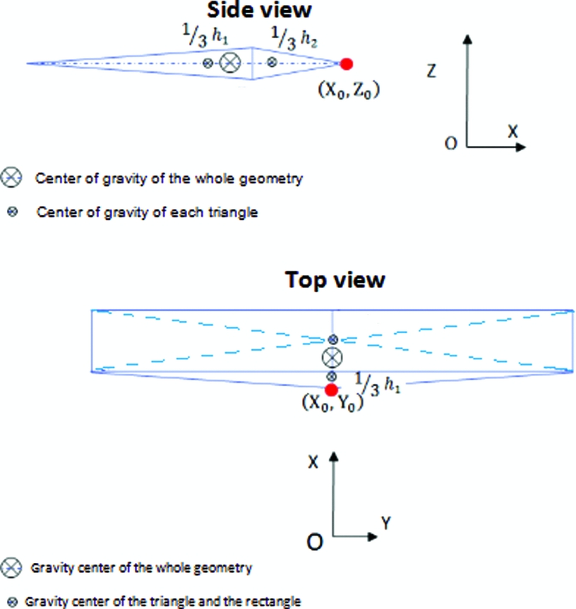
Figure 4. Top view and side view representation of the wing.
Once the gravity centres of the triangles and rectangles are found, the gravity centres of the wing projections on each plan are found separately by computing a weighted arithmetic mean of the gravity centre of all figures that constitute the projections. The weight use here is the area of each figure (so that only the geometry has the influence on the results) as illustrated in Equation (8) for the top view of the wing.
 $$
\begin{equation}
C{g_{TV}} = \frac{{{A_R}\;{*}\;C{g_R} + {A_T}\;{*}\;C{g_{T\ }}}}{{{A_R} + {A_T}}},
\end{equation}$$
$$
\begin{equation}
C{g_{TV}} = \frac{{{A_R}\;{*}\;C{g_R} + {A_T}\;{*}\;C{g_{T\ }}}}{{{A_R} + {A_T}}},
\end{equation}$$
where:
-
- AR and AT are, respectively, the areas of the rectangle R and the triangle T;
-
- CgTV , CgR and Cg T are, respectively, the centre of gravity of the whole top view of the wing, the rectangle and the triangle.
Subsequent to the calculation of the gravity centres of all the other parts of the UAS-S4 following the procedure described for the wing, the resulting coordinates are then expressed as the global axes system presented above, since they were first calculated relatively to various systems axes attached to the UAS part. Next, resulting coordinates are weighted with the mass of the corresponding UAS-S4 part (found in Section 2.1) and finally sum up to find the arithmetic mean that represents the centre of gravity coordinates of all the UAS-S4.
The experimental determination of the centre of gravity location of the UAS-S4 is shown in the next section.
2.3 Empirical estimation of the UAS-S4 mass moments of inertia-static method DATCOM(Reference Williams and Vukelich2)
All the equations(Reference Williams and Vukelich2) necessary for the mass moment of inertia calculation are coded and executed using MATLAB. As in Section 2.2, the principal moments of inertia of every part of the UAS-S4 are computed separately through DATCOM equations and then sum by the help of the theorem of ‘Huygens-Steiner’(Reference Soulé and Miller12). The estimation of the roll principal moment of inertia of the wing is shown below for the illustration of the procedure. It is based on Fig. 4, and is given by Equation (9).
 $$
\begin{equation}
{I_{OX\ {\rm{loca}}{{\rm{l}}_{\left( {{\rm{Wing}}} \right)}}}} = {M_{{\rm{wing}}}}{\left( {2\;{*}\;c} \right)^2}\frac{{{K_1}}}{{24}}\left( {\frac{{a + 3\;{*}\;b}}{{a + b}}} \right),
\end{equation}$$
$$
\begin{equation}
{I_{OX\ {\rm{loca}}{{\rm{l}}_{\left( {{\rm{Wing}}} \right)}}}} = {M_{{\rm{wing}}}}{\left( {2\;{*}\;c} \right)^2}\frac{{{K_1}}}{{24}}\left( {\frac{{a + 3\;{*}\;b}}{{a + b}}} \right),
\end{equation}$$
where I OX local(Wing) is the principal moment of inertia of the wing and M wing is the weight of the wing. The coefficient K 1 is empirically found using(Reference Williams and Vukelich2).
The roll principal moment of inertia of the wing calculated below is expressed in the local axes system attached to the wing centre of gravity. Every other principal moment of inertia (roll, pitch or yaw) of a UAS part is calculated following the same procedure and expressed in a system axis attached to the centre of gravity of the corresponding part.
Since we know that the distances between the various principal local system axes (attached to the centre of gravity of the UAS parts) and the global system axes are represented by the coordinates of the centres of gravity of the wing parts expressed in the global system axes (see Section 2.2), the moment of inertia could be expressed in the global axes system by the help of the ‘Huygens-Steiner’ theorem following Equation 10 and Equation 11. Figure 5 shows the illustration of the distances between the system axes
 $$
\begin{equation}
{I_{{x_j}\ {\rm{globa}}{{\rm{l}}_{\left( {{\rm{wing}}} \right)}}}} = {I_{{x_j}\ {\rm{loca}}{{\rm{l}}_{\left( {{\rm{wing}}} \right)}}}} + \mathop \sum \limits_{\begin{array}{@{}*{1}{c}@{}} {K = 1}\\ {k \ne j} \end{array}}^3 {M_{{\rm{wing}}}}\;{*}\;\left( {C{g_{{x_k}}}} \right)_{{\rm{wing}}}^2
\end{equation}$$
$$
\begin{equation}
{I_{{x_j}\ {\rm{globa}}{{\rm{l}}_{\left( {{\rm{wing}}} \right)}}}} = {I_{{x_j}\ {\rm{loca}}{{\rm{l}}_{\left( {{\rm{wing}}} \right)}}}} + \mathop \sum \limits_{\begin{array}{@{}*{1}{c}@{}} {K = 1}\\ {k \ne j} \end{array}}^3 {M_{{\rm{wing}}}}\;{*}\;\left( {C{g_{{x_k}}}} \right)_{{\rm{wing}}}^2
\end{equation}$$

Figure 5. Relative distances between the local system axes, the global system axes and the ‘Principal’ global system axes.
For the whole UAS, we have
 $$
\begin{equation}
{I_{{x_j}\ {\rm{global}}}} = \mathop \sum \limits_{i = {\rm{Wing}},\ {\rm{fuselage}},\ {\rm{landing}}\ {\rm{gear}}} \left( {{I_{{x_j}\ {\rm{loca}}{{\rm{l}}_i}}} + \mathop \sum \limits_{\begin{array}{@{}*{1}{c}@{}} {K = 1}\\ {k \ne j} \end{array}}^3 {M_i}\;{*}\;\left( {C{g_{{x_k}}}} \right)_i^2} \right),\vspace*{-15pt}
\end{equation}$$
$$
\begin{equation}
{I_{{x_j}\ {\rm{global}}}} = \mathop \sum \limits_{i = {\rm{Wing}},\ {\rm{fuselage}},\ {\rm{landing}}\ {\rm{gear}}} \left( {{I_{{x_j}\ {\rm{loca}}{{\rm{l}}_i}}} + \mathop \sum \limits_{\begin{array}{@{}*{1}{c}@{}} {K = 1}\\ {k \ne j} \end{array}}^3 {M_i}\;{*}\;\left( {C{g_{{x_k}}}} \right)_i^2} \right),\vspace*{-15pt}
\end{equation}$$
where:
-
- xj represents the axis (X, Y or Z) about which the mass moment of inertia I xj global is calculated;
-
- I xj global is the mass moment of inertia about xj axis and relative to the global axes system;
-
- Mi is the mass of the corresponding UAS-S4 part;
-
- (Cg xj ) i , for j=1 and i=1, is the X-coordinate of the centre of gravity of the wing.
Since we are interested in the principal moment of inertia of the whole UAS-S4, the result found in Equation (11) should be applied to the axes system attached to the centre of gravity of the UAS-S4 (principal global system axes). Equation 12 shows the calculation.
 $$
\begin{equation}
{I_{G{x_j}\ {\rm{global}}}} = {I_{{x_j}\ {\rm{global}}}} - {M_{{\rm{UAS}}}}\mathop \sum \limits_{\begin{array}{@{}*{1}{c}@{}} {\scriptstyle K = 1}\\ {\scriptstyle k \ne j} \end{array}}^3 \left( {C{g_{{x_j}}}} \right)_{{\rm{UAS}}}^2,
\end{equation}$$
$$
\begin{equation}
{I_{G{x_j}\ {\rm{global}}}} = {I_{{x_j}\ {\rm{global}}}} - {M_{{\rm{UAS}}}}\mathop \sum \limits_{\begin{array}{@{}*{1}{c}@{}} {\scriptstyle K = 1}\\ {\scriptstyle k \ne j} \end{array}}^3 \left( {C{g_{{x_j}}}} \right)_{{\rm{UAS}}}^2,
\end{equation}$$
where:
-
- I Gxj global (for j = 1) is the principal moment of inertia of the UAS-S4 about the X axis;
-
- (Cg xj ) (for j = 1) is the X-coordinate of the UAS-S4 centre of gravity.
3.0 EXPERIMENTAL DETERMINATION OF THE GRAVITY CENTRE OF THE UAS-S4 -PENDULUM METHOD
The coordinates of the centre of gravity are expressed relatively to the global axes system.
3.1 Z-coordinate of the centre of gravity (ZGUAV)
3.1.1 Theory and equations
The swinging gear proposed to tilt the UAS during the bench tests is shown in Fig. 6:

Figure 6. Swinging gear.
This bench test was carried out using the following procedure:
1st step: Hang the table horizontally on a beam as shown (Fig. 6).
2nd step: Place the UAS on the table, keeping the system (UAS and table) horizontal: the UAS’ and the table's centres of gravity are thus vertically aligned.
3rd step: Hang an extra weight m to unbalance the system (UAS + table) by tilting the assemblage around the X or Y axis, as shown in Fig. 6.
4th step: Redo the same bench test through the 3rd step, but without including the UAS–S4, which allows the Z-coordinate of the table's centre of gravity ZGt to be determined.
The moment equilibrium around an axis (Δ) is shown in Fig. 7, and leads to:
 $$
\begin{equation}
{\bm{M}_{\bm{M\vec{g}}/\Delta }} + {\bm{M}_{\bm{m\vec{g}}/\Delta }} = \ 0
\end{equation}$$
$$
\begin{equation}
{\bm{M}_{\bm{M\vec{g}}/\Delta }} + {\bm{M}_{\bm{m\vec{g}}/\Delta }} = \ 0
\end{equation}$$

Figure 7. Tilting of the UAS-S4 and table around the X or Y axis.

Figure 8. Z-positions of the gravity centres.
By replacing
 ${\bm{M}_{\bm{M\vec{g}}/\Delta }}\ $
and
${\bm{M}_{\bm{M\vec{g}}/\Delta }}\ $
and
 ${\bm{M}_{\bm{m\vec{g}}/\Delta }}\ $
by their expressions,
${\bm{M}_{\bm{m\vec{g}}/\Delta }}\ $
by their expressions,
 $$
\begin{equation}
M\;{*}\;{H_M}\sin \left( \theta \right) = m\left[ {{X_m}\cos \left( \theta \right) - {H_m}\sin \left( \theta \right)} \right]
\end{equation}$$
$$
\begin{equation}
M\;{*}\;{H_M}\sin \left( \theta \right) = m\left[ {{X_m}\cos \left( \theta \right) - {H_m}\sin \left( \theta \right)} \right]
\end{equation}$$
Equation (14) leads to the expression of Hm
 $$
\begin{equation}
{H_M} = \frac{m}{M}\left( {\frac{{{X_m}}}{{\tan\left(\theta \right)}} - {H_m}} \right)
\end{equation}$$
$$
\begin{equation}
{H_M} = \frac{m}{M}\left( {\frac{{{X_m}}}{{\tan\left(\theta \right)}} - {H_m}} \right)
\end{equation}$$
Since we know Hm , the centre of gravity of the system is derived, and further expressed in the global system axes, which are represented in Fig. 1,
 $$
\begin{equation}
{Z_{GS}} = {H_P} - {H_M},
\end{equation}$$
$$
\begin{equation}
{Z_{GS}} = {H_P} - {H_M},
\end{equation}$$
where:
-
-
 ${M_{M\vec{g}/\Delta }}$
is the moment created by the system weight around the axis Δ;
${M_{M\vec{g}/\Delta }}$
is the moment created by the system weight around the axis Δ; -
-
${M_{m\vec{g}/\Delta }}$
is the moment created by the extra weight m around the axis Δ; -
- HM is the vertical distance from the pivot to the centre of gravity of the system;
-
- Hm is the vertical distance from the pivot to the table;
-
- HP is the vertical distance from the pivot to the origin of the chosen axis;
-
- Xm is the horizontal distance from the extra weight to the centre of gravity of the system;
-
- m is the value of the extra weight;
-
- M is the value of the system's weight;
-
- Ө is the tilt angle;
-
- ZGS is the Z-coordinate of the system.


After finding the Z-coordinate of the table (ZGt ) as proposed in the 4th step, the projection of the three centres of gravity (UAV, table and system) upon the Z axis can be shown as:
From the barycenter properties, we obtain:
 $$
\begin{equation}
{Z_{{\rm{GUAS}}}} = \frac{{{Z_{Gs}}\;{*}\;\left( {{M_{{\rm{UAS}}}} + {M_t}} \right) - {Z_{Gt}}\;{*}\;{M_t}}}{{{M_{{\rm{UAS}}}}}},
\end{equation}$$
$$
\begin{equation}
{Z_{{\rm{GUAS}}}} = \frac{{{Z_{Gs}}\;{*}\;\left( {{M_{{\rm{UAS}}}} + {M_t}} \right) - {Z_{Gt}}\;{*}\;{M_t}}}{{{M_{{\rm{UAS}}}}}},
\end{equation}$$
where:
-
- ZGs is the Z coordinate of the centre of gravity of the system;
-
- ZGt is the Z-coordinate of the table;
-
- Z GUAS is the Z-coordinate of the UAS;
-
- M UAS is the weight of the UAS;
-
- Mt is the weight of the table.
During the experiment, the tilt angle Ө was measured with an accelerometer
3.1.2 Experimental setup
A wooden table was built as shown in Fig. 9 with the aim to perform the inertial tests. This table is 1.85 meters long and 1.22 meters wide. It is suspended from a steel beam structure by four underweight steel wires attached to two hinges hung on the upper beam. The beam structure is assumed to support about 115 kg, which is more than the total weight of the system (the UAS and the table). This arrangement can be seen in Fig. 9, in which the sensors (accelerometer and gyroscope) that allow us to get the pitch tilt angle caused by the extra load are identified. The sensor is set on the table so that its axes remain parallel to the axes of the table. It does not matter at which point the sensor is set because all the UAS and table points are subjected to the same speeds and the same displacements.

Figure 9. Experimental swinging gear with sensors and loads.
The UAS-S4 was arranged in two different positions, tilting around the X (roll) and about the Y (pitch) axes, as shown in Fig. 10.

Figure 10. UAS titling about the Y and X axes.
The tilted angles were measured for seven different loads and ten times for each load. The angle Ө appears to be proportional to the load for all the ten series of measure.
Before tilting the system using extra weights, it is first set horizontal by means of a bubble level. The sensor is then set on the table and initialised at zero degrees. Even if some initial small tilting angle is missed from the bubble level verification, the sensor will always measure the tilt angle variation when subjected to an extra weight because the initial angle will be taken as an offset.
From the titled angle, the Z-coordinate of the centre of gravity of the system (UAS + table) is computed as described in Equations (11) and (12). The Z-coordinate of the table is then calculated as the vertical distance from the origin of the global system axes to the table's half-thickness, because the table is a uniformly-distributed weight rectangle. And finally, the value of the Z-coordinate of the UAS-S4 is computed by using Equation (17); a summary of this procedure is described in Fig. 11.
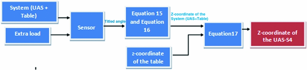
Figure 11. Procedure of calculation of the Z-coordinate of the UAS-S4.
3.2 Determination of the X-coordinate of the centre of gravity XGUAS
The X-coordinate of the UAS centre of gravity is found in two different ways:
-
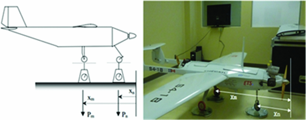
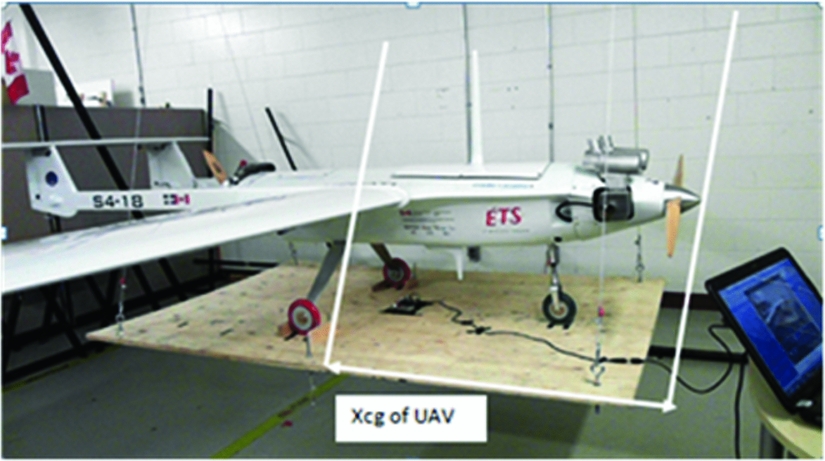
- Using the previous swinging gear set for determining the UAS Z-coordinate, the X-coordinate of the centre of gravity can be considered as the horizontal distance from the origin of the UAS to the centre of gravity of the table, shown in Fig. 12, since the centres of gravity of the table and the UAS one are vertically aligned.
-
- The second way to obtain the Xcg of the UAS is by the use of ‘scales’, as illustrated in Fig. 13.
Figure 12. X-coordinate of the gravity centre of the UAS.
Figure 13. UAS Xcg determination: theory and experimental implementation.

The X-coordinate is found by doing a weighted arithmetic mean of Xm and Xn :
 $$
\begin{equation}
{X_{{\rm{GUAS}}}} = \frac{{{X_m}{P_m} + {X_n}{P_n}}}{{{P_n} + {P_m}}},
\end{equation}$$
$$
\begin{equation}
{X_{{\rm{GUAS}}}} = \frac{{{X_m}{P_m} + {X_n}{P_n}}}{{{P_n} + {P_m}}},
\end{equation}$$
where:
-
- pn is the weight indicated by the scale n;
-
- p m is the weight indicated by the scale m;
-
- Xn is the X-coordinate of the position of the scale n;
-
- Xm is the X-coordinate of the position of the scale m.
The two distinct ways of calculating the Xcg of the UAS give close results with a relative difference of 4.05% (with the ‘scale's method’ taken as reference).
3.3 Determination of the Y-coordinate of the centre of gravity YGUAS
In theory, the Ycg of the UAS is assumed to be null because of the UAS symmetry, which is also verified experimentally. Since the centres of gravity of the table and the UAS are vertically aligned, their Y-coordinates are supposed to be the same, which can be determined as the horizontal distance from the origin to the half-width of the table is measured, as indicated on Fig. 14.

Figure 14. UAS-S4 Ycg experimental determination.
It was found that the Ycg of the UAS-S4 was nearly zero and close to 1.14 % of the total UAS-S4 span. The hypothesis of UAS-S4 symmetry is therefore validated.
3.4 Relative differences between the pendulum method results and the analytical predictions (Section 2.2)
Table 2 presents the relative errors between the analytical predictions of the UAS centre of gravity coordinates and the pendulum experimental results. The analytical predictions are taken as the reference in both comparisons. It is important to note that the analytical calculations are approximations, due to the complex shapes of the UAS S4-ETHECATL. Thus, the objective of the calculations in this section is to define an interval which bounds the actual value of the centre of gravity position.
Table 2 Results' comparisons of the centre of gravity position

For example, the relative errors are expressed as ratios between the difference between experimental and analytical CG position to the experimental CG position.
The relative errors are all less than 6%, and allow us to validate the analytical predictions of the UAS-S4’ gravity centre positions.
4.0 EXPERIMENTAL DETERMINATION OF THE MASS MOMENTS OF INERTIA OF THE UAS-S4 THOUGH THE PENDULUM METHOD
In this section, it is presented how the mass moments of inertia of the UAS-S4 are found through the pendulum method. The pendulum theories are explained in Sections 4.1 and 4.2, followed by the simulation of the pendulum models and the procedure of their comparisons with the experimental data, which in fact result in the estimation of the moment of inertia. The method of how the experimental data are gathered by the use of an accelerometer, a gyroscope and a magnetometer is also presented in this section.
The bifilar torsion type of pendulum theory is used for the Z axis mass moment of inertia calculation and the simple type of pendulum theory is used for the X and Y axes’ moments of inertia determination. The bifilar pendulum theory is presented in much more detail than the simple pendulum theory as it is more complicated; moreover, simple pendulum theory is more broadly understood and published.
4.1 Dynamic model of the bifilar pendulum
A bifilar (two wires) pendulum is a torsional pendulum composed by a test object, which is suspended by two parallel wires; the pendulum can oscillates about the vertical axis(Reference Matt and Muller14). The mass moment of inertia is computed by constructing the dynamic equation of the pendulum, which considers the dynamics of the damping, and the typical dimensions of the bifilar pendulum such as the length h and the separation displacement of the pendulum wires D Footnote 1 . The rotational angle in the horizontal plane is Ө, and Z is the vertical displacement, as shown on Fig. 15.

Figure 15. Bifilar pendulum diagrams(Reference Jardin16).
The dynamic model of the bifilar pendulum is obtained using the Lagrangian approach, so that we do not need to determine the constraint forces, which are not necessary for the determination of the mass moment of inertia. The dynamic model is developed for rotational motions of the centre of gravity of the system being tested, which includes the UAS-S4 and the table platform that supports it. The model considered the viscosity effects of the air and large angular displacements. The additional momentum of air that comes from the motion of air related to the rotation of an object of a large area is also computed. Figure 16 shows the displacements of the pendulum wires (which are representative of the twisting angle θ and the vertical displacement Z of the test object) when the pendulum is rotating around the Z axis.

Figure 16. Displacement of the bifilar pendulum wires.
The general form of the Lagrange equation of a motion is given by:
 $$
\begin{equation}
\frac{{{\bf d}}}{{{{\bf dt}}}}\left( {\frac{{{\bm{\partial }}{{\bf L}}}}{{{\bm{\partial }}{{\bf \dot{\theta }}}}}} \right) - \frac{{{\bm{\partial }}{{\bf L}}}}{{{\bm{\partial }}{{\bf \theta }}}} = {{\bf Q}},
\end{equation}$$
$$
\begin{equation}
\frac{{{\bf d}}}{{{{\bf dt}}}}\left( {\frac{{{\bm{\partial }}{{\bf L}}}}{{{\bm{\partial }}{{\bf \dot{\theta }}}}}} \right) - \frac{{{\bm{\partial }}{{\bf L}}}}{{{\bm{\partial }}{{\bf \theta }}}} = {{\bf Q}},
\end{equation}$$
where
 $$
\begin{equation}
{{\bf L}} = {{\bf T}} - {{\bf V}}
\end{equation}$$
$$
\begin{equation}
{{\bf L}} = {{\bf T}} - {{\bf V}}
\end{equation}$$
is the Lagrangian function in which T is the kinetic energy and V is the potential energy of the system. Q represents any non-conservative force. The total kinetic energy of the pendulum and the test object is composed by both rotational kinetic energy and translational kinetic energy:
 $$
\begin{equation}
{{\bf T}} = \frac{1}{2}{{\bf I}}{{{\bf \dot{\theta }}}^2} + \frac{1}{2}{{\bf m}}{{{\bf \dot{Z}}}^2},
\end{equation}$$
$$
\begin{equation}
{{\bf T}} = \frac{1}{2}{{\bf I}}{{{\bf \dot{\theta }}}^2} + \frac{1}{2}{{\bf m}}{{{\bf \dot{Z}}}^2},
\end{equation}$$
where
-
- I is the mass moment of inertia about the vertical axis;
-
- Ө is the angular displacement about the vertical axis;
-
-
$\dot{Z}$
is the is the rate of change of the vertical displacement Z vertical displacement of the test object.

An expression for the vertical displacement in terms of the angular displacement is obtained from Fig. 16, and is given by:
 $$
\begin{equation}
{{\bf Z}} = {{\bf h}}\left[ {1 - \sqrt {1 - \frac{{{{{\bf D}}^2}}}{{2{{{\bf h}}^2}}}(1 - {{\bf cos\theta }})\ } } \right]\ \
\end{equation}$$
$$
\begin{equation}
{{\bf Z}} = {{\bf h}}\left[ {1 - \sqrt {1 - \frac{{{{{\bf D}}^2}}}{{2{{{\bf h}}^2}}}(1 - {{\bf cos\theta }})\ } } \right]\ \
\end{equation}$$
Section 6.1 shows how Z is obtained from the geometry of Fig. 16. The rate of change of Z can be further calculated:
 $$
\begin{equation}
{{\bf \dot{Z}}} = \frac{{\left( {\frac{{{\bf h}}}{4}} \right){{\left( {\frac{{{\bf D}}}{{{\bf h}}}} \right)}^2}{{\bf sin}}\left( {{\bf \theta }} \right)}}{{\sqrt {1 - \left( {\frac{1}{2}} \right){{\left( {{{\bf D}}/{{\bf h}}} \right)}^2}\left[ {1 - {{\bf cos}}\left( {{\bf \theta }} \right)} \right]} }}{{\bf \dot{\theta }}}
\end{equation}$$
$$
\begin{equation}
{{\bf \dot{Z}}} = \frac{{\left( {\frac{{{\bf h}}}{4}} \right){{\left( {\frac{{{\bf D}}}{{{\bf h}}}} \right)}^2}{{\bf sin}}\left( {{\bf \theta }} \right)}}{{\sqrt {1 - \left( {\frac{1}{2}} \right){{\left( {{{\bf D}}/{{\bf h}}} \right)}^2}\left[ {1 - {{\bf cos}}\left( {{\bf \theta }} \right)} \right]} }}{{\bf \dot{\theta }}}
\end{equation}$$
The ratio of the translational kinetic energy to the rotational kinetic energy is derived from Equations (23) and (21), by the next equation:
 $$
\begin{equation}
\frac{{\left( {\frac{1}{2}} \right){{\bf m}}{{{{\bf \dot{Z}}}}^2}}}{{\left( {\frac{1}{2}} \right){{{\bf r}}^2}{{\bf m}}{{{{\bf \dot{\theta }}}}^2}}} = \left( {\frac{1}{{16}}} \right){\left( {\frac{{{\bf h}}}{{{\bf r}}}} \right)^2}{\left( {\frac{{{\bf D}}}{{{\bf h}}}} \right)^4}\frac{{{{\bf si}}{{{\bf n}}^2}\left( {{\bf \theta }} \right)}}{{1 - 1/2{{\left( {\frac{{{\bf D}}}{{{\bf h}}}} \right)}^2}\left[ {1 - \cos \left( {{\bf \theta }} \right)} \right]}}
\end{equation}$$
$$
\begin{equation}
\frac{{\left( {\frac{1}{2}} \right){{\bf m}}{{{{\bf \dot{Z}}}}^2}}}{{\left( {\frac{1}{2}} \right){{{\bf r}}^2}{{\bf m}}{{{{\bf \dot{\theta }}}}^2}}} = \left( {\frac{1}{{16}}} \right){\left( {\frac{{{\bf h}}}{{{\bf r}}}} \right)^2}{\left( {\frac{{{\bf D}}}{{{\bf h}}}} \right)^4}\frac{{{{\bf si}}{{{\bf n}}^2}\left( {{\bf \theta }} \right)}}{{1 - 1/2{{\left( {\frac{{{\bf D}}}{{{\bf h}}}} \right)}^2}\left[ {1 - \cos \left( {{\bf \theta }} \right)} \right]}}
\end{equation}$$
For the application of the pendulum theory, we consider the length h to be much greater than the separation displacement of the pendulum wire D. Therefore, the vertical translational kinetic energy is smaller than the rotational energy, and for this reason has been safely neglected. Thus, the kinetic energy of the bifilar pendulum can be written as given by Equation (25):
 $$
\begin{equation}
T = \frac{1}{2}I{\dot{\theta }^2}
\end{equation}$$
$$
\begin{equation}
T = \frac{1}{2}I{\dot{\theta }^2}
\end{equation}$$
The potential energy of the system is due to the vertical displacement and is expressed with the next equation:
 $$
\begin{equation}
V = mgZ
\end{equation}$$
$$
\begin{equation}
V = mgZ
\end{equation}$$
Then, by replacing T given by Equation (25), V given by Equation (26), and Z given by Equation (22), in Equation (20), we obtain:
 $$
\begin{equation}
L = \frac{1}{2}I{\dot{\theta }^2} - mgh[1 - \sqrt {1 - \frac{{{D^2}}}{{2{h^2}}}\left[ {1 - \cos \left( \theta \right)} \right]}
\end{equation}$$
$$
\begin{equation}
L = \frac{1}{2}I{\dot{\theta }^2} - mgh[1 - \sqrt {1 - \frac{{{D^2}}}{{2{h^2}}}\left[ {1 - \cos \left( \theta \right)} \right]}
\end{equation}$$
The damping associated with the pendulum's rotational motion was decomposed into both aerodynamic drag and viscous damping, which were considered in the expression of the following generalised force (see footnote Footnote 1).
 $$
\begin{equation}
Q = - {K_D}\dot{\theta }\left| {\dot{\theta }} \right| - C\dot{\theta },
\end{equation}$$
$$
\begin{equation}
Q = - {K_D}\dot{\theta }\left| {\dot{\theta }} \right| - C\dot{\theta },
\end{equation}$$
where KD and C are the damping parameters adjusted to match the experimental data with the simulated data.
By substituting Equation (27) and Equation (28) into Equation (19), and by performing the derivative operations with respect to the variable Ө, the following second-order nonlinear equation of motion is obtained for the bifilar pendulum.
 $$
\begin{equation}
\ddot{\theta } + \frac{{{K_D}}}{I}\dot{\theta }\left| {\dot{\theta }} \right| + \frac{C}{I}\dot{\theta } + \frac{{mg{D^2}}}{{4Ih}}\frac{{\sin \left( {\dot{\theta }} \right)}}{{\sqrt {1 - \left( {\frac{1}{2}} \right)\left( {\frac{{{D^2}}}{{{{(h)}^2}\left[ {1 - \cos \left( {\dot{\theta }} \right)} \right]}}} \right)} }} = 0
\end{equation}$$
$$
\begin{equation}
\ddot{\theta } + \frac{{{K_D}}}{I}\dot{\theta }\left| {\dot{\theta }} \right| + \frac{C}{I}\dot{\theta } + \frac{{mg{D^2}}}{{4Ih}}\frac{{\sin \left( {\dot{\theta }} \right)}}{{\sqrt {1 - \left( {\frac{1}{2}} \right)\left( {\frac{{{D^2}}}{{{{(h)}^2}\left[ {1 - \cos \left( {\dot{\theta }} \right)} \right]}}} \right)} }} = 0
\end{equation}$$
4.2 Dynamic model of the simple pendulum
As stated previously, the simple pendulum theory is much simpler than the theory of the bifilar pendulum theory. Our system is considered as a mass suspended from an inextensible wire of length h, such that the mass is free to swing from side to side in a vertical plane. Let Ө be the angle subtended between the string and the downward vertical axes as shown in Fig. 17.

Figure 17. Simple pendulum geometry.
From the fundamental principles of dynamics,
 $$
\begin{equation}
I\ddot{\theta } = \mathop \sum \limits {M_i}
\end{equation}$$
$$
\begin{equation}
I\ddot{\theta } = \mathop \sum \limits {M_i}
\end{equation}$$
where:
-
-
${M_{\vec{T}/\Delta }}$
is the torque caused by the tension
$\ \vec{T}$
around the axis Δ: -
-
${M_{\vec{P}/\Delta }}$
is the torque caused by the gravity force
$m\vec{g}$
around the axis Δ: -
-
${M_{\vec{F}/\Delta }}$
is the torque caused by the drag force
$\vec{F}$
around the axis Δ. -
-
$\vec{T}$
is the tension of wires; -
-
$\vec{g}$
is the gravitational acceleration; -
-
$\vec{F}$
contains both aerodynamic drag and viscous damping;


 $$\begin{equation}
{M_{\vec{T}/\Delta }} + {M_{\vec{P}/\Delta }} + {M_{\vec{F}/\Delta }} = I\ddot{\theta }
\end{equation}$$
$$\begin{equation}
{M_{\vec{T}/\Delta }} + {M_{\vec{P}/\Delta }} + {M_{\vec{F}/\Delta }} = I\ddot{\theta }
\end{equation}$$
From Ref. 15, we can write:
 $$
\begin{equation}-(C\dot{\theta } + {K_d}\dot{\theta }\left| {\dot{\theta }} \right|)h - mgh\sin \left( {\dot{\theta }} \right) = I\ddot{\theta }\ \ \ \
\end{equation}$$
$$
\begin{equation}-(C\dot{\theta } + {K_d}\dot{\theta }\left| {\dot{\theta }} \right|)h - mgh\sin \left( {\dot{\theta }} \right) = I\ddot{\theta }\ \ \ \
\end{equation}$$
Equation (32) can be rearranged under the following form
 $$
\begin{equation}
(C\dot{\theta } + {K_d}\dot{\theta }\left| {\dot{\theta }} \right|)h + mgh\sin \left( {\dot{\theta }} \right) + I\ddot{\theta } = 0
\end{equation}$$
$$
\begin{equation}
(C\dot{\theta } + {K_d}\dot{\theta }\left| {\dot{\theta }} \right|)h + mgh\sin \left( {\dot{\theta }} \right) + I\ddot{\theta } = 0
\end{equation}$$
Note that C * h and Kd * h can be considered as only two constants, C and Kd . The final equation of motion given by the simple pendulum theory is
 $$
\begin{equation}
\ddot{\theta } + \frac{C}{I}\dot{\theta } + \frac{{{K_d}}}{I}\dot{\theta }\left| {\dot{\theta }} \right| + \frac{{mgh}}{I}\sin \left( \theta \right) = 0
\end{equation}$$
$$
\begin{equation}
\ddot{\theta } + \frac{C}{I}\dot{\theta } + \frac{{{K_d}}}{I}\dot{\theta }\left| {\dot{\theta }} \right| + \frac{{mgh}}{I}\sin \left( \theta \right) = 0
\end{equation}$$
As it can be seen on Fig. 17, the system actually rotates about the (Δ) axis. So, after having the mass moment of inertia using Equation (34) (see Sections 4.2 and 4.3), we then have to apply the Huygens-Steiner theorem(Reference Soulé and Miller12) to obtain the principal moment of inertia about the principal axis of the UAS-S4. From the Huygens-Steiner theorem, the principal moment of inertia around x and y axes are obtained as follows:
 $$
\begin{equation}
{I_X} = {I_{{\rm{UA}}{{\rm{V}}_x}/\Delta }} - {m_{{\rm{UAV}}}}H_{{\rm{UAV}}}^2,
\end{equation}$$\\
$$
\begin{equation}
{I_X} = {I_{{\rm{UA}}{{\rm{V}}_x}/\Delta }} - {m_{{\rm{UAV}}}}H_{{\rm{UAV}}}^2,
\end{equation}$$\\
 $$
\begin{equation}
{I_Y} = {I_{{\rm{UA}}{{\rm{V}}_y}/\Delta }} - {m_{{\rm{UAV}}}}H_{{\rm{UAV}}}^2,
\end{equation}$$
$$
\begin{equation}
{I_Y} = {I_{{\rm{UA}}{{\rm{V}}_y}/\Delta }} - {m_{{\rm{UAV}}}}H_{{\rm{UAV}}}^2,
\end{equation}$$
-
- H GUAS is the vertical distance from the pivot to the centre of gravity of the UAS;
-
- m is the mass of the UAV;
-
- IX and IY are the principal moments of inertia about the x and y axes, respectively;
-
- I UAV X /Δ and I UAV y /Δ are the mass moment of inertia of the UAV about the Δ axis.
Since the table's mass moment of inertia is not negligible, the experiment should be redone with the table only. The mass moment of inertia of the table should then be subtracted from the total value of the mass moment of inertia of the system (UAS + table) before applying the Huygens-Steiner theorem.
4.3 Simulation of the pendulum models and comparison with experimental data
In Refs Reference Soulé and Miller12 and Reference Dubois13, the bench tests using the pendulums were conducted while maintaining small angular displacements, by assuming that the damping effect would not cause significant errors to the resulting inertia estimates. that assumption has the benefit of requiring only simple measurements by use of the period of the oscillations T, but the simplicity gained by linearisation and by neglecting the damping terms usually comes at the expense of measurement accuracy.
4.3.1 Simulated model of the pendulums
Based on the dynamic models of simple and bifilar pendulums developed in Sections 4.1 and 4.2, we created MATLAB models which can be solved using any differential equation solver. The bifilar pendulum equation of motion (Equation (27)) is then solved in 50 seconds, by the means of Runge-Kutta algorithm. Figure 18 shows the numerical results obtained for the angle and speed variations with time.

Figure 18. Simulated angle (radian) and speed (radian per second) motion of the bifilar pendulum.
4.3.2 Comparison between experimental data and simulated model's behaviour to find experimental mass moment of inertia
The dynamic models of the pendulums, when simulated, gives us data (simulated angle and speed) that depends on their unknown parameter (I, C and Kd ) and that can be directly compared to experimental data by the means of the ‘algorithms of minimization’.
The aim of the ‘algorithms of minimization’ is to look for and find the unknown parameters (I, C and Kd ) of the dynamic models that make the simulated resulting data match the experimental ones; the experimental data are obtained from sensors following Section 4.3.3.
The minimisation is made by the means of the following steps. First, we need to calculate both the angle and the speed square errors between the experimental and the simulated data at each time step; then add them and obtain the unknown parameters’ error function, which is the function we want to minimise:
 $$
\begin{equation}
{\rm{Error}}\left( {Kd,C,I} \right) = \mathop \sum \limits_{t = 0}^n {({\theta _t} - {\bar{\theta }_t})^2} + {({\dot{\theta }_t} - {\bar{\dot{\theta }}_t})^2},
\end{equation}$$
$$
\begin{equation}
{\rm{Error}}\left( {Kd,C,I} \right) = \mathop \sum \limits_{t = 0}^n {({\theta _t} - {\bar{\theta }_t})^2} + {({\dot{\theta }_t} - {\bar{\dot{\theta }}_t})^2},
\end{equation}$$
where
-
- θ t is the experimental angle position at time t;
-
-
${\bar{\theta }_t}\ $
is the simulated angle position at time t;
-
-
${\dot{\theta }_t}\ $
is the experimental speed at time t;
-
-
${\bar{\dot{\theta }}_t}$
is the simulated speed at time t.


From Fig. 19,
 $$
\begin{equation}
{\rm{Error}}\left( {Kd,C,I} \right) = \mathop \sum \limits_{t = 0}^{50} {({\theta _t} - {\bar{\theta }_t})^2} + {({\dot{\theta }_t} - {\bar{\dot{\theta }}_t})^2}
\end{equation}$$
$$
\begin{equation}
{\rm{Error}}\left( {Kd,C,I} \right) = \mathop \sum \limits_{t = 0}^{50} {({\theta _t} - {\bar{\theta }_t})^2} + {({\dot{\theta }_t} - {\bar{\dot{\theta }}_t})^2}
\end{equation}$$

Figure 19. Relative error function variation with time (experimental versus numerical data).
The MATLAB code ‘ga (entry function)’ is used to locate the local minimum of the entry function using genetic algorithms. It is written as:
 $$
\begin{equation}
{\left[ {{K_d},\ C,\ I} \right]_1} = ga\left( {{\rm{error}},\;\ n{\mathop{\rm var}} s,\ LB,\ UB} \right)
\end{equation}$$
$$
\begin{equation}
{\left[ {{K_d},\ C,\ I} \right]_1} = ga\left( {{\rm{error}},\;\ n{\mathop{\rm var}} s,\ LB,\ UB} \right)
\end{equation}$$
where
-
- Kd , C and I are the variables of the error function;
-
- error is the function for which we calculate the minimum value;
-
- n var s is the number of variables (3 in our case); and
-
- LB and UB are the lower and upper bounds of the search interval.
The values obtained using ‘ga’ are those that verify
 $$
\begin{equation}
{\rm{error}}\left( {Kd,C,I} \right) \cong 0,
\end{equation}$$
$$
\begin{equation}
{\rm{error}}\left( {Kd,C,I} \right) \cong 0,
\end{equation}$$
since the minimum of the positive error function should obviously be approximately equal to zero. The ‘ga’ function can find an approximate minimum in a very large interval, but not accurately. However, it does allow the algorithm to move its solution closer to the desired minimum. In order to be more accurate, the ‘fminsearch’ function is used as follows.
 $$
\begin{equation}
{\left[ {{K_d},\ C,\ I} \right]_2} = f\min \;{\rm{search}}\left( {{\rm{error}},{{\left[ {{K_d},\ C,\ I} \right]}_1}} \right)
\end{equation}$$
$$
\begin{equation}
{\left[ {{K_d},\ C,\ I} \right]_2} = f\min \;{\rm{search}}\left( {{\rm{error}},{{\left[ {{K_d},\ C,\ I} \right]}_1}} \right)
\end{equation}$$
‘fminsearch’ starts at the point [Kd , C, I]1 and returns a value [Kd , C, I]2 that is a local minimiser of the error function. “fminsearch” is not appropriate to find a minimum of functions defined on a large interval. It is very accurate, but implies the condition that the starting point is not too far from the minimiser (otherwise, it may drift); this is the reason why we used the ‘ga’ function beforehand. The two functions ‘ga’ and ‘fminsearch’ produce a graph that is shown in Fig. 20:

Figure 20. The Error Function variation with three parameters (Kd, C, I). Search field of ‘ga’ (in red) and ‘fminsearch’ (in yellow) functions.
-
- The red area represents the ‘ga’ function's search field;
-
- The yellow area is search field of ‘fminsearch’ function.
At the end of the optimisation using the combination of the ‘ga’ and ‘fminsearch’ functions, the local minimum is obtained with a relative error less than 10−4.
4.3.3 Obtainment of experimental data from sensors
Gathering experimental data requires the use of an accelerometer, a gyroscope, a magnetometer and a microcontroller board. These sensors and their use are described in the next sub-sections.
4.3.3.1 Accelerometer
The accelerometer is a device that measures the acceleration of the object to which it is connected. It measures the linear acceleration, plus 1g straight upwards due to its weight. For example, if it is set flat, it will indicate 0g on the X and Y axes, and 1g on the Z axis (the vertical (3D) axis).
We used the IMU-MPU6050, which is a digital and three-axis accelerometer with a full-scale range of ± 2g and 16,384 LSB/g of sensitivity.
The accelerometer enables us to obtain both pitch (oscillation about the Y axis) and roll (oscillation about the X axis) accelerations, but not the yaw acceleration (oscillation about the Z axis); Since our system is not subjected to forces other than gravitation, when it rotates about the Z axis, none of the forces will change on any axis, as the gravitational force does not change on any axis. The values of the tilt angles for pitch and roll motions shown in Fig. 21 are computed with the following equations:
 $$
\begin{equation}
{\theta _x} = a\tan \left( {\frac{{{A_y}}}{{{A_Z}}}} \right),
\end{equation}$$\\
$$
\begin{equation}
{\theta _x} = a\tan \left( {\frac{{{A_y}}}{{{A_Z}}}} \right),
\end{equation}$$\\
 $$
\begin{equation}
{\theta _y} = a\tan \left( {\frac{{{A_x}}}{{{A_Z}}}} \right),
\end{equation}$$
$$
\begin{equation}
{\theta _y} = a\tan \left( {\frac{{{A_x}}}{{{A_Z}}}} \right),
\end{equation}$$
-
- θ x is the pitch angle;
-
- θ y is the roll angle;
-
- Ax is the X-coordinate of the accelerometer output;
-
- Ay is the Y-coordinate of the accelerometer output;
-
- Axz is the acceleration projection on the XZ plane.

Figure 21. Rotation of the accelerometer about its Y axis.
The accelerometer has the disadvantage of being too noisy. However, its output does not drift at all over time; that means the output values of the accelerometer always oscillate around the right value of the acceleration but with some noises.
4.3.3.2 Gyroscope
Unlike accelerometers, gyroscopes measure the angular velocity about each axis. They can be used to obtain roll, pitch and yaw angles.
A three-axes gyroscope that has 6 degrees of freedom (6 DOF) is used, which is integrated on the same board as the IMU-MPU6050 accelerometer. This gyroscope has a full-scale range of ∓250 °/s, a sensitivity of 131 LSB/(°/S) and determines, as previously mentioned, the roll, pitch and yaw angles.
The tilt angles around each of the three axes can be computed by integrating data output from the gyroscope, as follows:
 $$
\begin{equation}
W = \frac{{d\theta }}{{dt}},
\end{equation}$$\\
$$
\begin{equation}
W = \frac{{d\theta }}{{dt}},
\end{equation}$$\\
 $$
\begin{equation}
{\theta _n} = {\theta _{n - 1}} + {W_n}\Delta t
\end{equation}$$
$$
\begin{equation}
{\theta _n} = {\theta _{n - 1}} + {W_n}\Delta t
\end{equation}$$
Unfortunately, because of the successive integrations, the gyroscope adds up all of the possible noises and keeps them over time, which explains why it quickly drifts. However, also due to the multiple integrations, the angle signal from a gyroscope is rather smooth, but this advantage is not enough to be able to rely solely on its results.
4.3.3.3 Magnetometer
Magnetometers are used to obtain the yaw angle. They work by detecting the magnetic fields produced by the hot rotating iron core at the centre of the earth. The vector of the earth's magnetic field has a component parallel to the earth's surface that always points toward the magnetic north pole, making it possible to express yaw. The vertical component always points downwards, with a precise angle depending on the location. In Montreal, the magnetic inclination is 70°22’(Reference Ozyagcilar15), and this value allows us to verify the calibration.
We used a triple-axis magnetometer breakout MAG3110 that has a full-scale range of 100µT and a sensitivity of 0.1µT/LSB.
As mentioned above, the horizontal component of the local magnetic field Hh always points to the Magnetic North (Fig. 22). This horizontal component is measured only by the X and Y axes. The yaw angle is computed with the following equation:
 $$
\begin{equation}
{\rm{yaw}} = a\tan \left( {\frac{{{X_h}}}{{{Y_h}}}} \right)
\end{equation}$$
$$
\begin{equation}
{\rm{yaw}} = a\tan \left( {\frac{{{X_h}}}{{{Y_h}}}} \right)
\end{equation}$$

Figure 22. Determining the yaw angle from a magnetometer.
It is important to note that the magnetometer must be held flat (zero degree of inclination) during the yaw measurement procedure in order to reliable data. If it is not set flat, there is a way to compensate for the tilt with accelerometer measurements, but that procedure is not worth noting here, since our device is kept flat throughout all the readings. As with accelerometers, magnetometers do not drift over time but they are noisy.
4.3.3.4 Sensors' calibration
The sensors used here all feature three 16-bit analog-to-digital converters (ADCs) for digitizing their outputs in the form of counts. The counts are then converted to engineering units, such as acceleration and speed, by applying the sensitivity coefficient on the raw output, as seen in Equation (47):
 $$
\begin{equation}
{\rm{value}} = \left( {{\rm{raw}}\ {\rm{output}}} \right)\;{*}\;{\rm{sensitivity}}\
\end{equation}$$
$$
\begin{equation}
{\rm{value}} = \left( {{\rm{raw}}\ {\rm{output}}} \right)\;{*}\;{\rm{sensitivity}}\
\end{equation}$$
The offsets can then be computed. For the accelerometer and the gyroscope, the removal operations are relatively simple. A sample of 2,000 measurements is produced while maintaining the device fixed and flat. In theory, the output values measured in the gyroscope axes should all be equal to zero, as the device is not moving. The X and Y outputs from the accelerometer should be equal to zero and the Z outputs should be equal to 1g since the device is held flat.
Therefore, for the X, Y and Z gyroscope axes and for the X and Y accelerometer axes, the offset is written as
 $$
\begin{equation}
\text{offset} = \frac{1}{{2000}}\;{*}\;\mathop \sum \limits_{i = 1}^{2000} {({\rm{output}})_i}
\end{equation}$$
$$
\begin{equation}
\text{offset} = \frac{1}{{2000}}\;{*}\;\mathop \sum \limits_{i = 1}^{2000} {({\rm{output}})_i}
\end{equation}$$
and for the Z accelerometer axis the offset is written as follows:
 $$
\begin{equation}
{\text{offset}} = \frac{1}{{2,000}}\;{*}\;\mathop \sum \limits_{i = 1}^{2,000} \left[ {{{({\rm{output}})}_i} - 1} \right]
\end{equation}$$
$$
\begin{equation}
{\text{offset}} = \frac{1}{{2,000}}\;{*}\;\mathop \sum \limits_{i = 1}^{2,000} \left[ {{{({\rm{output}})}_i} - 1} \right]
\end{equation}$$
After computing the offsets, they are always subtracted from the ‘value’ determined in Equation (45) before estimating the pitch, roll and yaw angles, as shown in Equations (42), (43), (45), and (46).
The determination of the magnetometer offsets is more complicated. In theory, distortions of the earth's magnetic field result from external magnetic influences that are generally classified as either ‘hard’ or ‘soft iron’ effects(Reference Ozyagcilar15). If no distorting effects are present, the rotation of the magnetometer in all directions and the plotting of the resulting data on the X axis versus the Y axis and versus the Z axis will result in a sphere centred on (0,0,0).
‘Hard iron’ distortion is due to a permanently magnetised ferromagnetic component around a device. It can be identified by an offset of the origin of the actual sphere output from (0,0,0), as shown in Fig. 23.

Figure 23. Hard iron distortion exhibited by a constant offset in the X, Y and Z axes.
The ‘hard iron offsets’ are determined as the distance (on each axis) between the centre of the sphere and the (0,0,0) point. Figure 24 shows the same measurements (as the ones shown in Fig. 23) after their correction for hard iron distortion. The new sphere is centred at the (0,0,0) point.

Figure 24. Hard iron compensation.
The ‘soft iron effect’ is defined as a magnetic field that interferes with the normally un-magnetised ferromagnetic components around the device(Reference Jardin16). A soft iron distortion is typically exhibited as a perturbation of the ideal sphere into an ellipsoid. Luckily, in our experiment, the soft iron effect is neglected since a plot of measurements without any soft iron correction is already a sphere.
4.3.3.5 Complementary Filter
None of the sensors used here can be completely ‘trusted’ on their own for the precision of the measurements. One of the simplest ways to correct them is by using a complementary filter (high- and low-pass filters). Complementary filters are designed so that that the strength of one sensor is used to overcome the weaknesses of another, mutually complementary sensor. Figure 25 shows how the three sensors outputs are filtered and fused together.

Figure 25. Complementary filter design.
The accelerometer data are first low-pass filtered to erase all the high-frequency noises, making sure that only the constant signal value and the fluctuations caused by the accelerometer movements (which is the low-frequencies variation) are taken into account. The gyroscope data are high-pass filtered because from the gyroscope, we are interested in the short-term signal variation rather than the actual signal value which, as we know, drift over the time. The complementary task concerns of combining the accelerometer and gyroscope data as shown below:
 $$
\begin{equation}
\hspace*{-10pt}{\rm{\ angl}}{{\rm{e}}_{{\rm{comp}}\left( {n + 1} \right)}} = 0.02\;{*}\;{\rm{angl}}{{\rm{e}}_{{\rm{acc}}/{\rm{magn}}}} + 0.98\;{*}\;\left( {{\rm{angl}}{{\rm{e}}_{{\rm{comp}}\left( n \right)}} + {\rm{spee}}{{\rm{d}}_{{\rm{gyro}}}}\;{*}\;dt} \right),
\end{equation}$$
$$
\begin{equation}
\hspace*{-10pt}{\rm{\ angl}}{{\rm{e}}_{{\rm{comp}}\left( {n + 1} \right)}} = 0.02\;{*}\;{\rm{angl}}{{\rm{e}}_{{\rm{acc}}/{\rm{magn}}}} + 0.98\;{*}\;\left( {{\rm{angl}}{{\rm{e}}_{{\rm{comp}}\left( n \right)}} + {\rm{spee}}{{\rm{d}}_{{\rm{gyro}}}}\;{*}\;dt} \right),
\end{equation}$$
where:
-
- anglecomp(n) is the angle outputs by the complementary filter at the time step n;
-
- angleacc/magn is the low-pass filtered accelerometer or magnetometer angle;
-
- speedgyro * dt is the high pass filtered gyroscope angle.
This complementary filter has the benefit of being easy to code and not very processor-intensive. Its results are given in Fig. 26:

Figure 26. Results obtained after filtering.

Figure 27. Swing test about the Y, X and Z axes.

Figure 28. Angle variation vs time (top) and velocity vs time (bottom).
where:
-
- the green line is the accelerometer or the magnetometer signal;
-
- the red line is the gyroscope signal;
-
- the blue line is the complementary filtered signal.
Figure 26 illustrates the results obtained after filtering. Due to the numerical integrations, the gyroscope has drifted over time and the accelerometer is noisy throughout all the motion. Both results from the gyroscope and accelerometer are further combined to obtain a very good filtered signal. These remarks would be also valid if the accelerometer signal (measuring the pitch or the roll) was replaced by the magnetometer signal (measuring the yaw).
4.4 Additional momentum of air
The UAS-S4’ additional momentum of air is the moment of inertia caused by the air dragged by the UAS while oscillating during the experiment. It is computed in accordance with Ref. 12. When the additional force is incorporated in the equations of motion (Equations (29) and (34)), its effect is the same as if the actual mass moment of inertia of the pendulum system was increased. The form of the equation of motion does not change, but the mass moment of inertia I (in Equations (29) and (34)) must be understood to represent the total measured mass moment of inertia of the system, including the additional air momentum. The mass moment of inertia of the test object is obtained by subtracting the inertia due to the additional mass from the total moment of inertia (see footnote Footnote 1).
 $$
\begin{equation}
I = {I_{{\rm{total}}}} - {I_{{\rm{air}}}}
\end{equation}$$
$$
\begin{equation}
I = {I_{{\rm{total}}}} - {I_{{\rm{air}}}}
\end{equation}$$
4.4.1 Additional momentum of air about the X axis
From Ref. 12, the additional momentum of air about the X axis is due to the wings and the horizontal tail. The X axis is in the plane of symmetry of both the wings and the tail surface. The equation for the additional mass moment of inertia for this case is:
 $$
\begin{equation}
{I_a} = \frac{{k'\rho \pi {c^2}{b^3}}}{{48}},
\end{equation}$$
$$
\begin{equation}
{I_a} = \frac{{k'\rho \pi {c^2}{b^3}}}{{48}},
\end{equation}$$
where c is the chord and b is the span of each part. The coefficient k’ depends on the ratio c/b and varies with the aspect ratio as shown in Ref. 12.
For the UAV S4-18 ETHECATL k’ = 0.88 for the wings and 0.75 for the horizontal tail. The additional mass moment of inertia is computed for each component and the sum of the moments of inertia for the wings and the horizontal tail appears to be 1.11% of the mass moment of inertia of the UAS-S4 and air.
4.4.2 Additional momentum of air about Y axis
About the Y axis, the additional moment of inertia is assumed to be contributed by the fuselage and the horizontal tail. For the horizontal area of the fuselage, an equivalent rectangle is considered, with its length equal to that of the fuselage and width equal to the square root of the mean square of the fuselage width(Reference Soulé and Miller12).
As the Y axis is parallel to the chord but displaced from the centre of gravity of the fuselage by the distance ‘l’, the expression used for the additional moment of the fuselage is:
 $$
\begin{equation}
{I_{af}} = \left[ {\frac{{k'\rho \pi {c^2}{b^3}}}{{48}} + \frac{{k\rho \pi {c^2}b{l^2}}}{4}} \right],
\end{equation}$$
$$
\begin{equation}
{I_{af}} = \left[ {\frac{{k'\rho \pi {c^2}{b^3}}}{{48}} + \frac{{k\rho \pi {c^2}b{l^2}}}{4}} \right],
\end{equation}$$
where k is assumed to be equal to 1 and k’ equals 0.68 for the fuselage(Reference Soulé and Miller12). The Y axis is parallel to the span of the horizontal tail, therefore the additional mass for the horizontal tail about the Y axis is computed as:
 $$
\begin{equation}
{I_{af}} = \left[ {\frac{{k\rho \pi {c^2}b{l^2}}}{4}} \right],
\end{equation}$$
$$
\begin{equation}
{I_{af}} = \left[ {\frac{{k\rho \pi {c^2}b{l^2}}}{4}} \right],
\end{equation}$$
where k depends on the ratio c/b and varies as shown in Ref. Reference Soulé and Miller12. The coefficient k for the horizontal tail is close to 0.7. The total additional mass about the Y axis is approximately 9.97% of the mass moment of inertia of the UAS and air.
The value of the additional moment computed of air also includes the additional momentum of air for the axis translation (for X and Y axes). It should be finally subtracted from the value obtained with the Huygens-Steiner theorem.
4.5 Experimental procedure
The pendulum experimental method presented in Sections 4.1-4.4 is now applied for the measurement of the mass moment of inertia of the UAV S4-18 Ehecatl. The same table is used to swing the UAS about the three axes.
The initialisation procedure consists of collecting data for 1 minute with the system at rest in order to verify the pitch, roll and yaw alignments. If the alignments are good, the motion could start. The speeds and the angles are then recorded by the sensors until the angles are less than 0.5 degrees.
After gathering the experimental data, these data are matched with the simulated motion data using the ‘algorithm of minimization’ as proposed in the Section 4.3.2. This allows us to obtain the total value of mass moment of inertia about the axis of oscillation. Next, the mass moment of inertia of the table is computed in the same way and then subtracted from the previous values obtained for the system (UAS and table).
It is not necessary to compute the additional air momentum caused by the motion of the table because it is already present in the moment of inertia computed for the system (table and the UAS), and the one computed for the table only. Following the subtraction of these two values, the additional air momentum of the table is eliminated.
As no axis transposition is necessary for the bifilar suspension (oscillation takes place about the Z axis), the Huygens-Steiner theorem is only applied for the motion around the other two axes, X and Y (as shown in Equations (35) and (36) to obtain the UAS’ principal moment of inertia. Figure 29 recapitulates the whole procedure. Table 4 shows the relative errors of the numerical and experimental data of the measurements of the principal moment of inertia of a rectangular cuboid.

Figure 29. Calculation of the principal moment of inertia of the UAS-S4.
4.6 Relative differences between the pendulum experimental results and the Datcom method results (Section 2.3)
Table 3 presents the relative errors between the results obtained by DATCOM empirical method and the ones obtained through the pendulum method. The percentage calculations take DATCOM result as reference.
Table 3 Relative errors obtained for the principal moment of inertia of the UAS-S4

Table 4 Relative errors of the numerical and experimental data of the measurements of the principal moment of inertia of a rectangular cuboid (see Sections 3.4 and 4)
4.7 Mass moment of inertia of an object of uniform density
The mass moment of inertia of a rectangular cuboid was computed both analytically and experimentally to determine the accuracy of the experimental method.
5.0 CONCLUSION
A process for locating the centre of gravity and experimentally measuring the mass moment of inertia of test objects with the pendulum method were described and applied to the UAS S4-Ethecatl. Aerodynamic drag, viscous damping and large-angle oscillations were accounted for in the experiment. Owing to the effect of ambient air, the total moment of inertia obtained directly through application of the pendulum method was reduced by the additional moment of air. The experiment appears to be precise with an error less than 7.8% on average. The results of recent flight tests conducted by Hydra Technologies could validate the results and the precision of our experimental method, which could then be applied on many other UASs in the future. The sensors installed for this research will certainly be used for other applications.
6.0 APPENDICES
6.1 VERTICAL DISPLACEMENT Z
We want to express the vertical displacement in terms of the angular displacement in accordance with the bifilar pendulum's geometry.
From Fig. 30, we have
 $$\begin{eqnarray*}
Z &=& h - c\\
Z &=& h - \sqrt {{h^2} - {b^2}}
\end{eqnarray*}$$
$$\begin{eqnarray*}
Z &=& h - c\\
Z &=& h - \sqrt {{h^2} - {b^2}}
\end{eqnarray*}$$

Figure 30. Bifilar pendulum's geometry.
with:
 $$\begin{eqnarray*}
&&\left\{ {\begin{array}{@{}*{1}{c}@{}} {{b^2} = {a^2} + {{(\frac{D}{2}\sin \theta )}^2}}\\ { = > \ \ {b^2} = \frac{{{D^2}}}{4}{{(1 - cos\theta )}^2} + {{(\frac{D}{2}\sin \theta )}^2}}\\ { = > {b^2} = \frac{{{D^2}}}{4}(1 - 2cos\theta + {{(cos\theta )}^2} + {{(\sin \theta )}^2})}\\ { = > {b^2} = \frac{{{D^2}}}{2}\left( {1 - cos\theta } \right)} \end{array}} \right.\\
Z &=& h - \sqrt {{h^2} - \frac{{{D^2}}}{2}\left( {1 - \cos \left( \theta \right)} \right)} \\
Z &=& h\left[ {1 - \sqrt {1 - \frac{{{D^2}}}{{2{h^2}}}(1 - \cos \theta )} } \right]
\end{eqnarray*}$$
$$\begin{eqnarray*}
&&\left\{ {\begin{array}{@{}*{1}{c}@{}} {{b^2} = {a^2} + {{(\frac{D}{2}\sin \theta )}^2}}\\ { = > \ \ {b^2} = \frac{{{D^2}}}{4}{{(1 - cos\theta )}^2} + {{(\frac{D}{2}\sin \theta )}^2}}\\ { = > {b^2} = \frac{{{D^2}}}{4}(1 - 2cos\theta + {{(cos\theta )}^2} + {{(\sin \theta )}^2})}\\ { = > {b^2} = \frac{{{D^2}}}{2}\left( {1 - cos\theta } \right)} \end{array}} \right.\\
Z &=& h - \sqrt {{h^2} - \frac{{{D^2}}}{2}\left( {1 - \cos \left( \theta \right)} \right)} \\
Z &=& h\left[ {1 - \sqrt {1 - \frac{{{D^2}}}{{2{h^2}}}(1 - \cos \theta )} } \right]
\end{eqnarray*}$$
6.1.1 The Arduino Uno set-up
The Arduino Uno is the acquisition board that was used to obtain data from the sensors.
To set all the sensors together, we need to connect:
-
- the Arduino Ground (GND) to the MPU6050 GND;
-
- the Arduino 3.3v to the MPU6050 VCC;
-
- the Arduino analog 4(I2C data) to the MPU6050 SDA;
-
- the Arduino analog 5(I2C clock) to the MPU6050 SCL;
-
- the Arduino GND to the MAG3110 GND;
-
- the Arduino 3.3v to the MAG3110 VCC;
-
- the Arduino analog 4(I2C data) to the MAG3110 SDA;
-
- the Arduino analog 5(I2C clock) to the MAG3100 SCL.
Figure 31 shows these connections for the Arduino circuit board.

Figure 31. Circuit board.
ACKNOWLEDGEMENTS
We would like to thank the Hydra Technologies team in Mexico for their continuous support, and especially Mr. Carlos Ruiz, Mr. Eduardo Yakin and Mr. Alvaro Gutierrez Prado. In addition, the authors would like to thank to the NSERC and Government of Canada for the funding received for the Canada Research Chair in Aircraft Modeling and Simulation Technologies. We would also like to thank to the Canada Founding of Innovation CFI, to the MDEIE and to Hydra Technologies for the UAS-S4 acquisition.