


1. Introduction
Our objective in this paper is to study the following initial value problem associated with the time-fractional derivative with biharmonic operator
 \begin{equation} \begin{cases} \displaystyle \partial^{\alpha}_{0|t} u(t,x) + \Delta^{2} u(t,x)=G(t,x,u), & \mbox{in}\quad\mathbb{R}^{+}\times\mathbb{R}^{N}, \\ \displaystyle u(0,x)= u_0(x), & \mbox{in} \quad \mathbb{R}^{N}, \end{cases} \end{equation}
where  $0<\alpha <1$ and, for an absolutely continuous in time function
  $w$, the definition the Caputo time-fractional derivative operator
  $\partial ^{\alpha }_{0|t}$ is introduced in [Reference Caputo12] as follows:
 \begin{equation} \partial^{\alpha}_{0|t} w(t)= \frac{1}{\Gamma(1-\alpha)} \int_0^{t} (t-s)^{-\alpha} \frac{{\textrm{d}}w}{{\textrm{d}}s} \,{\textrm{d}}s, \end{equation}
here, we assume that the integration makes sense  $\Gamma$ is the Gamma function. The main equation in (P) contains the biharmonic operator
  $\Delta ^{2}$ which is often called higher-order parabolic equations and began to receive widespread attention for their surprising and unexpected properties. More importantly, the higher-order parabolic equations can be used to model many problems in applications, namely, the study of weak interactions of dispersive waves, the theory of combustion, the phase transition, the higher-order diffusion. The most common higher-order parabolic equation is probably the polyharmonic heat equation, especially, the fourth-order heat equation or also called the biharmonic heat equation. The current paper only considers the source function
  $G$ to be in two nonlinear cases: the exponential nonlinear type and the Cahn–Hilliard equation form.
1.1 Fractional partial differential equations
Over the last few decades, the theory of fractional derivatives has been well developed. As a result, the fractional partial differential equations (FPDEs) have also been studied more and more widely. These new kinds of PDEs have many unexpected properties and numerous applications in many applied and theoretical fields of science and engineering. This is why many researchers have shown a big interest in the study of FPDEs. Recently, there have been many interesting studies concerning diffusion equations with non-local time derivatives and time-fractional derivatives. We can refer the reader to some interesting papers on FPDEs, for example, Caraballo et al. [Reference Xu, Zhang and Caraballo42, Reference Xu, Zhang and Caraballo43], Zacher [Reference Zacher44, Reference Zacher45], Vespri et al. [Reference Dipierro, Valdinoci and Vespri17], Nane et al. [Reference Asogwa, Mijena and Nane5, Reference Tuan, Nane, O'Regan and Phuong37], Carvalho and Planas [Reference de Carvalho-Neto and Planas13], Dong and Kim [Reference Dong and Kim20, Reference Dong and Kim21], Tuan et al. [Reference Tuan, Ngoc, Zhou and O'Regan38, Reference Tuan, Au and Xu39] and references therein. We especially consider the interesting studies [Reference Dipierro, Pellacci, Valdinoci and G. Verzini18, Reference Kemppainen, Siljander, Vergara and Zacher27, Reference Vergara and Zacher40] because our views in approaching the problem are somewhat similar to theirs. Indeed, the works [Reference Dipierro, Pellacci, Valdinoci and G. Verzini18, Reference Kemppainen, Siljander, Vergara and Zacher27] study time-fractional problems with second-order differential operators through the fundamental solution. Although in [Reference Dipierro, Pellacci, Valdinoci and G. Verzini18], Dipierro and co-authors establish existence and uniqueness for the solution in an appropriate functional space, and in [Reference Kemppainen, Siljander, Vergara and Zacher27], Zacher et al. consider decay estimates of the solution. The study [Reference Vergara and Zacher40] investigates the same problem as [Reference Kemppainen, Siljander, Vergara and Zacher27] but the results are provided in a bounded domain of  $\mathbb {R}^{N}$ and applied to investigate some specific examples corresponding to their kernel
  $k$. When considered these studies, we found some important remarks about appropriate functional spaces to study the fundamental solution (remark 2.1). Motivated by those, we made some detailed observations for ours. On the contrary, our main contributions are the results for models with the biharmonic operators whose properties are somewhat different from the second-order ones. Furthermore, we focus on studying specific effects of different types of nonlinearity to our mild solution. To provide a clearer view, we will present specific discussions below.
1.2 Discussion on problem (P) with exponential nonlinearity
The source function  $G$ is the exponential nonlinearity satisfying
  $G(0)=0$ and
 \begin{equation} \left|G(u)-G(v)\right|\le L|u-v|\left({|u|^{m-1}\,{\textrm{e}}^{\kappa|u|^{p}}+|v|^{m-1}\,{\textrm{e}}^{\kappa|v|^{p}}}\right), \end{equation}
for every  $u,v\in \mathbb {R}, m>2\text { or }m=1,p>1$ and
  $L$ is a positive constant independent of
  $u,v.$ In the following, we will discuss in more detail why we chose this function
  $G$ as in (1.2).
• In terms of mathematical theory: It was common knowledge that when we consider the IVP for the classical Schrödinger equations with the polynomial nonlinearity
 $u|u|^{p-1},\ p\in (1,\infty )$ and an initial data function in $H^{s}(\mathbb {R}^{N}),\ s\in [0,N/2)$, the value $\mathbf {\bar {c}}=1+4(N-2s)^{-1}$ is called the critical exponent. Then, the power case $p$ of the nonlinear function is equal to (respectively less than) $\mathbf {\bar {c}}$ is called the critical case (respectively subcritical case). However, when considering the functional space $H^{\frac {N}{2}}(\mathbb {R}^{N})$, the critical value $\mathbf {\bar {c}}$ will be larger than any power exponent of the polynomial nonlinearity. Hence, the nonlinear functions of exponential type grow higher than any kind of a power nonlinearity at infinity and also vanishes like a power at zero, which can be seen as the critical nonlinearity of this case. This is also one of the reasons why exponential nonlinearity has been studied by many mathematicians not only for both the Schrödinger equation and some other types of PDEs. To provide an overview of this kind of nonlinearity, let us recall some related studies. The framework introduced above is based on results in [Reference Nakamura and Ozawa33]. In this study, Nakamura and Ozawa study the small data global $H^{N/2}(\mathbb {R}^{N})$-solution of the IVP for the Schrödinger equations with the exponential nonlinearity. The IVP for heat equations with this type of nonlinearity was considered in [Reference Ioku24]. In [Reference Ioku24], under the smallness assumption on the initial data in the Orlicz space, Ioku has shown the existence of a global-in-time solution of the semilinear heat equations. Under the smallness condition of initial data, decay estimates and the asymptotic behaviour for global-in-time solutions of a semilinear heat equation with the nonlinearity given by $f(u)=|u|^{4/N}u\,{\textrm {e}}^{u^{2}}$ was investigated in [Reference Furioli, Kawakami, Ruf and Terraneo22] by Furioli et al. For more results about the exponential nonlinearity, we refer the reader to [Reference Bartolucci, Leoni, Orsina and Ponce6, Reference Dinh, Keraani and Majdoub16, Reference Ioku, Ruf and Terraneo25, Reference Petropoulou34] and the references therein.
• In terms of application: These exponential nonlinearities as in (1.2) are not only investigated for the nonlinear Schrödinger equations but also for other types of PDEs because of many applications in phenomena modelling. Let us mention two well-known applications in combustion theory as follows. The first one is the IVP for the equation
$u_t-\Delta u=k\,{\textrm {e}}^{u}$, it can be used to model the ignition solid fuel. The second one is the description of the small fuel loss steady-state model by the IVP associated with equation $-\Delta u=k\,{\textrm {e}}^{\frac {u}{(1+\varepsilon u)}}.$ More applications and details can be found in [Reference Bebernes and Eberly7, Reference Kazdan and Warner26] and references therein.• Contributions, challenges and novelties: To the best of our knowledge, FPDEs with nonlinearities of exponential type have not been studied yet. Our study can be seen as one of the first results in this topic. Due to the nonlinearity of exponential type, it is not possible to apply
$L ^{p}-L^{q}$ estimates of some previous studies [Reference Andrade and Viana3, Reference De Andrade and Viana4] to our current problem. In contrast to the case $s>N/2,$ the embedding ${L^{\infty }(\mathbb {R}^{N})}\hookleftarrow H^{N/2}$ is not true, and in view of Trudinger–Moser's inequality, we obtain the embeddings $H^{N/2}(\mathbb {R}^{N})\hookrightarrow {L^{\Xi }(\mathbb {R}^{N})}\hookrightarrow {L^{q}(\mathbb {R}^{N})}$ for any $p\le q<\infty ,$ where ${L^{\Xi }(\mathbb {R}^{N})}$ is the Orlicz space with the function $\Xi (z)={\textrm {e}}^{|z|^{p}}-1$ (see definition 2.5). To deal with the exponential type, we shall use the Orlicz space and the embeddings between it and the usual Lebesgue spaces. However, since our problem is considered in the whole space $\mathbb {R}^{N}$, the embedding ${L^{q}(\mathbb {R}^{N})}\hookrightarrow {L^{p}(\mathbb {R}^{N})}$ does not hold anymore when $q>p$. For Orlicz spaces in classical derivatives, the use of the standard smoothing effect of the exponential resolution and Taylor expansion operators play important roles. However, they are not available for problems with time-fractional derivatives. The appearance of the Mittag-Leffler function and the Gamma function also caused a lot of difficulties in setting up some needed estimates related to the Orlicz space for problem (P). Fortunately, thanks to the results shown in [Reference Mainardi, Mura and Pagnini32], the standard smoothing effect can be achieved with a presentation via the M-Wright function of the Mittag-Leffler function. We can also overcome some of the difficulties caused by the Gamma function with some special inequalities. Our main results in this section are briefly described as follows:
• In the regular case of
$u_0 (u_0\in {L^{p}(\mathbb {R}^{N})}\cap {C_0(\mathbb {R}^{N})}),$ we can derive that our mild solution blows up at a finite time or the maximal time that ensures the unique existence of the solution is infinity.• With the assumption of the initial value in the space
${L^{\Xi }(\mathbb {R}^{N})}$, the local-in-time existence of mild solution can be obtained by a fixed point argument without any smallness assumptions on the initial function. Furthermore, under the stronger assumption that $u_0\in {L^{\Xi }_{0}(\mathbb {R}^{N})}$, the global well-posed results for the solution will be established. To achieve this goal, we have to use the techniques introduced by Chen et al. [Reference Chen, Gao, Garrido-Atienza and Schmalfuß14], and weighted spaces to deal with the singular term of the mild solution.


1.3 Discussion on problem (P) with Cahn–Hilliard source term
In this subsection, we introduce and discuss problem (P) with another source  $G(u)\equiv \Delta F(u)$, here
  $F$ denotes the derivative of double-well potential; in general, we consider a cubic polynomial like
  $F(u)=u^{3}-u.$ For the case
  $\alpha =1$, problem (P) is reduced to the standard Cahn–Hilliard equation. The Cahn–Hilliard equation was proposed for the first time by Cahn and Hilliard [Reference Cahn and Hilliard11], and is one of the most often studied problems of mathematical physics, which describes the process of phase separation of a binary alloy below the critical temperature. More recently, it has appeared in nano-technology, in models for stellar dynamics, as well as in the theory of galaxy formation as a model for the evolution of two components of inter-galactic material (see [Reference Blowey and Elliott8]). Let us mention some previous studies on the standard Cahn–Hilliard equations with derivatives of integer order. In [Reference Abels, Bosia and Grasselli1], the authors considered a Cahn–Hilliard equation which is the conserved gradient flow of a nonlocal total free energy functional. Bosch and Stoll [Reference Bosch and Stoll9] proposed a fractional inpainting model based on a fractional-order vector-valued Cahn–Hilliard equation [Reference Caffarelli and Muler10]. We can list many classical papers related to the study of Cahn–Hilliard equation, see, e.g.Dlotko [Reference Dlotko19], Temam [Reference Temam36], Akagi [Reference Akagi, Schimperna and Segatti2], Zelik [Reference Cherfils, Miranville and Zelik15, Reference Kostianko and Zelik28] and the references therein.
• Contributions, challenges and novelties: As we mentioned above, when we consider the FPDEs in
$\mathbb {R}^{N}$, the relationship between two spaces ${L^{p}(\mathbb {R}^{N})}$ and ${L^{q}(\mathbb {R}^{N})}$ with $p\neq q$ is not fulfilled. Specifically, one of the greatest challenges, when we investigate the Cahn–Hilliard equations, is to deal with a nonlinearity of the form $G(u)=\Delta F(u)$. Due to the appearance of the Laplacian, when handling the existence and the uniqueness of the mild solution by the successive approximations method and Young's convolution inequality, the property of ${\textrm {d}}/{\textrm {d}}x\left ({f(x)*g(x)}\right )$ needs to be applied to make the second-order derivative of the solution representation operator appear. This novelty in this case is setting up the key estimates as in lemma 2.3. It is worth noting that even when we have the main tools available, it is still not an easy task to prove our desired existence results. Besides, when finding the regularity results, we have to estimate the higher-order derivative of the solution representation operators. By learning about the results and techniques of [Reference Liu, Wang and Zhao29, Reference Luca, Goldman and Strani30], we found a way to obtain the local-in-time existence and uniqueness result for problem (P) with the Cahn–Hilliard source. The global-in-time existence of the solution is a difficult topic and will probably be studied in a forthcoming study. The section about the time-fractional Cahn–Hilliard equation in this study includes:• to find the solution representation by the Fourier transform and some related properties;
• to establish some useful linear estimates;
• to prove the existence, uniqueness and regularity of local-in-time solution by using the Picard sequence method and the smallness assumption for the initial data function.


1.4 The outline
In § 2, we demonstrate an approach to present the formula of the mild solution and, based on it, we establish some important linear estimates. Also in this section, we introduce some notations and definitions related to the so-called Orlicz space, a generalization of Lebesgue spaces and some useful embeddings between them. In § 3, we investigate problem (P) with the exponential nonlinearities under two separate assumptions on the initial datum function. In particular, for the first assumption, we show that the mild solution exists on  $[0,\infty )$ or blows up in a finite time. The local existence and the global-in-time well-posedness of the solution will be stated under the second assumption of the initial function. The main results on the problem with the second type of nonlinearity source function will be analysed in § 4. In general, by using the smallness assumption on the initial function, we derive the local-in-time existence and uniqueness of the mild solution for the IVP associated with the time-fractional Cahn–Hilliard equation. Furthermore, the regularity result will also be proved.
2. Preliminaries
2.1 Generalized mild solution
It is well known that for the following IVP involving a classical homogeneous biharmonic equation
 \[ \begin{cases} \partial_t \varphi(t,x)+\Delta^{2} \varphi(t,x)=0, & \text{in}\quad\mathbb{R}^{+}\times\mathbb{R}^{N},\\ \varphi(t,x)=\varphi_0(x), & \text{in}\quad\{0\}\times\mathbb{R}^{N}, \end{cases} \]
the solution is given by
 \[ \varphi(t,x)=\left[{\mathcal{F}^{{-}1}\left({{\textrm{e}}^{{-}t|\xi|^{4}}}\right)*\varphi_0}\right](x)=\left[{(2\pi)^{\frac{-\mathbb{N}}{2}}\int_{\mathbb{R}^{N}}\,{\textrm{e}}^{i< \xi,x>{-}t|\xi|^{4}}\,{\textrm{d}} \xi}\right]*\varphi_0(x), \]
where the Fourier transform and its inverse are denoted by  $\mathcal {F},\mathcal {F}^{-1},$ respectively, and
  $<\xi ,x>= \sum _{j=1}^{N} \xi _j x_j, (\xi ,x)\in \mathbb {R}^{2N}.$ We recall the following lemma for the kernel
  $\mathscr K (t,x)= \mathcal {F}^{-1} ({\textrm {e}}^{-t|\xi |^{4}} ).$
Lemma 2.1 Suppose that  $p\ge 1$. Then, for any
  $t>0$ we have
 \[ \|\mathscr{K}(t )\|_{L^{p}}\le c_p t^{-\frac{N}{4})(1-\frac{1}{p})}, \quad\|D^{m} \mathscr{K}(t )\|_{L^{p}}\le c_{p,m} t^{-\frac{N}{4})(1-\frac{1}{p})-\frac{m}{4}}. \]
In view of the above approach, to find the representation for the mild solution to problem (P), we consider the IVP for a homogeneous time-fractional biharmonic equation as follows:
 \begin{equation} \begin{cases} \displaystyle \partial^{\alpha}_{0|t}\varphi(t,x)+\Delta^{2}\varphi(t,x)=0, & \mbox{in}\quad\mathbb{R}^{+}\times\mathbb{R}^{N},\\ \displaystyle \varphi(0,x)=\varphi_0(x), & \mbox{in} \quad \mathbb{R}^{N}. \end{cases} \end{equation}
Applying the Laplace transform,  $\mathscr {L}$, with respect to the time variable to the first equation of (2.1), we have
 \[ z^{\alpha}\mathscr{L}\{\varphi\}(z,x)-z^{\alpha-1}\varphi_0(x)+\Delta^{2}\mathscr{L}\{\varphi\}(z,x)=0. \]
Then, by assuming that  $\varphi _0$ belongs to some appropriate spaces and using the Fourier transform with respect to the spatial variable, the following equation holds
 \[ z^{\alpha}\mathcal{F}(\mathscr{L}\{\varphi\})(z,\xi)-z^{\alpha-1}\mathcal{F}(\varphi_0)(\xi)+|\xi|^{4}\mathcal{F}(\mathscr{L}\{\varphi\})(z,\xi)=0. \]
By some simple calculations, one has
 \[ \mathcal{F}(\mathscr{L}\{\varphi\})(z,\xi)=\frac{z^{\alpha-1}}{z^{\alpha}-|\xi|^{4}}. \]
We now use the inverse Laplace transform to obtain
 \[ \mathcal{F}(\varphi)(t,\xi)=\widehat{\varphi}(t,\xi)=E_{\alpha,1}\left({-t^{\alpha}|\xi|^{4}}\right)\widehat{\varphi_0}(\tau). \]
Thanks to the Duhamel principle, the Fourier transform of the solution to problem (P) is given by
 \[ \widehat{u}(t,\xi)= E_{\alpha,1} ({-}t^{\alpha} |\xi|^{4})\widehat{u_0}(\xi)+ \int_0^{t} (t-s)^{\alpha-1} E_{\alpha,\alpha} (- (t-\tau)^{\alpha} |\xi|^{4}) \widehat{G(u)} (\tau,\xi) \,{\textrm{d}}\tau. \]
Where  $E_{\alpha ,1},E_{\alpha ,\alpha }$ are Mittag-Leffler functions. Using the inverse Fourier transform, we obtain
 \begin{align*} u(t,x)&= \left[{\mathcal{F}^{{-}1} \Big(E_{\alpha,1} ({-}t^{\alpha} |\xi|^{4})\Big)*u_0}\right](x)\\ &\quad + \int_0^{t} \mathcal{F}^{{-}1} \Big((t-\tau)^{\alpha-1} E_{\alpha,\alpha} ({-}t^{\alpha} |\xi|^{4})\Big)(x)*G(u(\tau,x))\,{\textrm{d}} \tau, \end{align*}
where we have used the fact that  $\widehat {f*g}(\tau )=\widehat {f}(\tau )\widehat {g}(\tau )$. For convenience, we denote
 \begin{equation} \mathbb{K}_{1,\alpha} (t,x)= \mathcal{F}^{{-}1} \Big(E_{\alpha,1} ({-}t^{\alpha} |\xi|^{4})\Big)(x),\quad \mathbb{K}_{2,\alpha}(t,x)= \mathcal{F}^{{-}1} \Big(t^{\alpha-1} E_{\alpha,\alpha} ({-}t^{\alpha} |\xi|^{4})\Big)(x), \end{equation}
and set operators  $\mathbb {Z}_{i,\alpha } (i=1,2)$ as follows:
 \[ \mathbb{Z}_{i,\alpha}(t,x) v(t,x)= \mathbb{K}_{i,\alpha} (t,x) * v(t,x)= \int_{\mathbb{R}^{N}} \mathbb{K}_{i,\alpha} (t,x-y) v(t,y)\,{\textrm{d}}y ,\quad i=1,2. \]
Then, we rewrite our solution formula in a concise form
 \begin{align} u(t,x)= \mathbb{Z}_{1,\alpha}(t,x)u_0(x)+ \int_0^{t} \mathbb{Z}_{2,\alpha}(t-\tau,x)G(u(\tau,x))\,{\textrm{d}} \tau. \end{align}
Remark 2.1 It is worth noting that the above approach is similar to the common one used to construct the fundamental solution for time-fractional problems with second-order differential operators. Let us provide some remarks from interesting studies about functional spaces in which the fundamental kernels are considered.
(i) The work [Reference Dipierro, Pellacci, Valdinoci and G. Verzini18] studies an evolution problem with the Caputo derivative of order
$\alpha \in (0,1)$ and the Dirac delta distribution centred at $x = 0$ (the initial data function). The solution formula of this problem is given by
Then, based on it, the authors have made very interesting comments about functional spaces to which the Fourier transform of the solution belongs. More precisely, they showed that\[ u(\xi,t)=\mathcal{F}^{{-}1}\Big(E_{\alpha,1}\big[(a-4\pi^{2}b|\xi|^{2})t^{\alpha}\big]\Big),\quad a\ge 0,\ b>0. \]$\mathcal {F}u(\cdot ,t)$ is in ${L^{p}(\mathbb {R}^{N})}$ if and only if $p\in (N/2,\infty )$. This result implies some different case for functional spaces depending on the dimension $N$.(ii) In [Reference Kemppainen, Siljander, Vergara and Zacher27, § 3] the authors proved optimal decay estimates for solutions to a time-fractional diffusion equation. Their solution is as follows:
From the above, they deduced as a conclusion that\[ u(x,t)=\int_{\mathbb{R}^{N}}Z(x-y,t)u_0(y)\,{\textrm{d}}y,\quad \text{where}\ \mathcal{F}\{Z\}(\xi,t)=E_{\alpha,1}\big(-|\xi|^{2}t^{\alpha}\big). \]$Z(t)$ fails to belong to ${L^{p}(\mathbb {R}^{N})}$ for $N\ge 4$ and $p\ge \frac {N}{(N-2)}$.


These facts are important when using the fundamental solution to establish well-posed results. In the spirit of the above studies, we also present some similar comments on the estimates for kernels  $\mathbb {K}_{1,\alpha },\mathbb {K}_{2,\alpha }$ in remark 2.3.
In order to achieve the standard smoothing effect of  $\mathbb {Z}_{i,\alpha } (i=1,2)$, we also present the mild solution in another form. To this end, we recall the definition of Mittag-Leffler function via the M-Wright type function as follows:
 \begin{align} E_{\alpha,1}({-}z)= \int_0^{\infty} \mathcal{M}_\alpha (\zeta)\,{\textrm{e}}^{{-}z\zeta} \,{\textrm{d}}\zeta,\quad E_{\alpha,\alpha}({-}z)=\int_0^{\infty} \alpha\zeta \mathcal{M}_\alpha (\zeta)\,{\textrm{e}}^{{-}z\zeta} \,{\textrm{d}}\zeta,\quad z \in \mathbb{C}. \end{align}
Then, we have the second type representation of the solution of problem (P1)
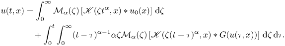 \begin{align} u(t,x)&=\int_{0}^{\infty}\mathcal{M}_{\alpha}(\zeta)\left[{\mathscr K (\zeta t^{\alpha},x)*{u}_0(x)}\right]\,{\textrm{d}} \zeta \nonumber\\ &\quad+\int_{0}^{t}\int_{0}^{\infty}(t-\tau)^{\alpha-1}\alpha \zeta\mathcal{M}_{\alpha}(\zeta)\left[{\mathscr K (\zeta(t-\tau)^{\alpha},x)*G(u(\tau,x))}\right]\,{\textrm{d}} \zeta \,{\textrm{d}}\tau. \end{align}
Due to the great impact of the operator  $\mathbb {K}_{1,\alpha },\mathbb {K}_{2,\alpha }$ to our results for mild solutions, we present the following Theorem which can be seen as the combination of theorem 3.1, theorem 3.2 and remark 1.6 of [Reference Wang, Chen and Xiao41].
Theorem 2.2 Let  $X={L^{p}(\mathbb {R}^{N})} (1\le p<\infty )$ or
  $X=C_0(\mathbb {R}^{N}).$ Then,
  $\mathbb {Z}_{1,\alpha }(t)$ and
  $t^{1-\alpha }\mathbb {Z}_{2,\alpha }(t)$ are bounded linear operators on
  $X$. In addition, for
  $w\in X$,
  $t\to \mathbb {Z}_{1,\alpha }(t),\ t\to t^{1-\alpha }\mathbb {Z}_{2,\alpha }(t)$ are continuous functions from
  $\mathbb {R}^{+}$ to
  $X$.
$X$.
Remark 2.2 In fact, although theorems of [Reference Wang, Chen and Xiao41] can be applied for other spaces in which  $\Delta ^{2}$ generates a strongly continuous semigroup, in this study, we only focus on the spaces
  ${L^{p}(\mathbb {R}^{N})} (1\le p<\infty )$ and
  $C_0(\mathbb {R}^{N})$.
We continue the study by introducing some useful  $L^{p}$-estimates for the kernel
  $\mathbb {K}_{1,\alpha },\mathbb {K}_{2,\alpha }$ by the following lemma.
Lemma 2.3 Let  $p\ge 1$ and
  $k\in \mathbb {N}$ be constants such that
  $k<4-N\left ({1-\frac {1}{p}}\right ).$ Then, there exist two constants
  $\mathscr C_{k,p}, \overline { \mathscr C_{k,p}}$ which depend only on
  $\alpha$ and
  $N$, such that
 \begin{equation} \Big\| D^{k} \mathbb{K}_{1,\alpha} (t ) \Big\|_{L^{p}} \le \mathscr C_{k,p} (\alpha, N) t^{-\frac{\alpha N}{4}-\frac{\alpha k }{4}+ \frac{\alpha N}{4p}} \end{equation}
and
 \begin{equation} \Big\| D^{k} \mathbb{K}_{2,\alpha} (t ) \Big\|_{L^{p}} \le \overline{ \mathscr C_{k,p}} (\alpha, N) t^{\alpha-\frac{\alpha N}{4}-1+\frac{\alpha N}{4p}-\frac{\alpha k}{4}}. \end{equation}
Proof. Step 1. To verify the first inequality
In this step, we deal with the term  $\mathbb {K}_{1,\alpha } (t,x)$. In fact, the representation of
  $\mathbb {K}_{1,\alpha } (t,x)$ and (2.4) together with Fubini's theorem allow us to deduce
 \begin{align*} \mathbb{K}_{1,\alpha} (t,x) &= \mathcal{F}^{{-}1} \Big(E_{\alpha,1} ({-}t^{\alpha} |\xi|^{4})\Big)(x)=\left({2\pi}\right)^{{-}N} \int_{\mathbb{R}^{N}}\,{\textrm{e}}^{i <\xi, x>} \Big(E_{\alpha,1} ({-}t^{\alpha} |\xi|^{4})\Big)\,{\textrm{d}}\xi\\ &= \left({2\pi}\right)^{{-}N}\int_{\mathbb{R}^{N}} \,{\textrm{e}}^{i <\xi, x>} \Big(\int_0^{\infty} \mathcal{M}_\alpha (\zeta) \,{\textrm{e}}^{{-}t^{\alpha} \zeta |\xi|^{4}} \,{\textrm{d}}\zeta \Big)\,{\textrm{d}}\xi\\ &=\left({2\pi}\right)^{{-}N} \int_0^{\infty} \int_{\mathbb{R}^{N}} \mathcal{M}_\alpha (\zeta) \,{\textrm{e}}^{i <\xi, x>} \,{\textrm{e}}^{{-}t^{\alpha} \zeta |\xi|^{4}} \,{\textrm{d}}\xi \,{\textrm{d}}\zeta. \end{align*}
By setting  $\xi = \vartheta (t^{\alpha } \zeta )^{-\frac {1}{4}}$, it is straightforward that
  ${\textrm {d}}\xi = (t^{\alpha } \zeta )^{-\frac {N}{4}} \,{\textrm {d}}\vartheta$ and
  $|\xi |^{4}= (t^{\alpha } \zeta )^{-1} |\vartheta |^{4}$. Let us denote by
 \begin{equation} \overline{\mathscr B}_k(y)= \int_{\mathbb{R}^{N}} |\vartheta|^{k}\,{\textrm{e}}^{i < y,\vartheta> } \,{\textrm{e}}^{-|\vartheta|^{4}} \,{\textrm{d}}\vartheta,\quad k\ge 0. \end{equation}
By some simple transformations, we find the following equality
 \begin{align*} \mathbb{K}_{1,\alpha} (t,x)&= \int_0^{\infty} \int_{\mathbb{R}^{N}} (t^{\alpha} \zeta )^{-\frac{N}{4}} \mathcal{M}_\alpha (\zeta) \,{\textrm{e}}^{{i <\vartheta, x> t^{-\frac{\alpha}{4}} \zeta ^{-\frac{1}{4}}}} \,{\textrm{e}}^{-|\vartheta|^{4}} \,{\textrm{d}}\vartheta \,{\textrm{d}}\zeta \\ &= t^{-\frac{\alpha N}{4}}\Bigg( \int_0^{\infty} \zeta^{-\frac{N}{4}} \mathcal{M}_\alpha (\zeta) \int_{\mathbb{R}^{N}} \,{\textrm{e}}^{{i <\vartheta, x> t^{-\frac{\alpha}{4}} \zeta ^{-\frac{1}{4}}}} \,{\textrm{e}}^{-|\vartheta|^{4}} \,{\textrm{d}}\vartheta \,{\textrm{d}} \zeta \Bigg)\\ &= t^{-\frac{\alpha N}{4}} \int_0^{\infty} \zeta^{-\frac{N}{4}} \mathcal{M}_\alpha (\zeta) \overline{\mathscr B}_0 (x (t^{\alpha} \zeta )^{-\frac{1}{4}} ) \,{\textrm{d}}\zeta. \end{align*}
If we set  $x (t^{\alpha } \zeta )^{-\frac {1}{4}} =z,$ then it follows immediately that
  ${\textrm {d}}x= (t^{\alpha } \zeta )^{\frac {N}{4}} \,{\textrm {d}}z$. Applying Minkowski's inequality in integral form, we have
 \begin{align*} &\left(\int_{\mathbb{R}^{N}}\left|\int_0^{\infty} \zeta^{-\frac{N}{4}} \mathcal{M}_\alpha (\zeta) \overline{\mathscr B}_0 (x (t^{\alpha} \zeta )^{-\frac{1}{4}} ) \,{\textrm{d}}\zeta\right|^{p}\,{\textrm{d}}x\right)^{\frac{1}{q}}\\ &\quad \le\int_0^{\infty}\left(\int_{\mathbb{R}^{N}}\left| \zeta^{-\frac{N}{4}} \mathcal{M}_\alpha (\zeta) \overline{\mathscr B}_0 (x (t^{\alpha} \zeta )^{-\frac{1}{4}} ) \right|^{p}\,{\textrm{d}}x\right)^{\frac{1}{q}}\,{\textrm{d}} \zeta. \end{align*}
It follows that
 \begin{align*} \Big\|\mathbb{K}_{1,\alpha} (t,x)\Big\|_{L^{p}} &\le t^{-\frac{\alpha N}{4}} \int_0^{\infty} \Bigg( \int_{\mathbb{R}^{N}} \Big| \zeta^{-\frac{N}{4}} \mathcal{M}_\alpha (\zeta) \overline{\mathscr B}_0 \left(x (t^{\alpha} \zeta )^{-\frac{1}{4}} \right) \Big| ^{p} (t^{\alpha} \zeta )^{\frac{N}{4}} \,{\textrm{d}}z\Bigg)^{\frac{1}{p}} \,{\textrm{d}} \zeta \\ &= t^{-\frac{\alpha N}{4}+\frac{\alpha N}{4p}} \left( \int_0^{\infty} \zeta^{\frac{N}{4p}-\frac{N}{4}} \mathcal{M}_\alpha (\zeta) \,{\textrm{d}}\zeta \right) \Bigg( \int_{\mathbb{R}^{N}} \Big| \overline{\mathscr B}_0 (z) \Big|^{p} \,{\textrm{d}}z \Bigg)^{\frac{1}{p}}. \end{align*}
By setting  $\Theta _{p,N}=( \int _{\mathbb {R}^{N}} \Big | \overline {\mathscr B}_0 (z) \Big |^{p} \,{\textrm {d}}z)^{\frac {1}{p}}$ and using lemma A.2, we obtain the following bound
 \begin{equation} \Big\|\mathbb{K}_{1,\alpha} (t )\Big\|_{L^{p}} \le \frac{\Theta_{p,N} \Gamma(\frac{N}{4p}-\frac{N}{4}+1) }{\Gamma(\frac{\alpha N}{4p}-\frac{\alpha N}{4}+1) } t^{-\frac{\alpha N}{4}+\frac{\alpha N}{4p}} . \end{equation}
Next, let us consider the derivative of  $\mathbb {K}_{1,\alpha } (t,x)$. It is easy to see that
 \[ \Big\|D \mathbb{K}_{1,\alpha} (t )\Big\|_{L^{p}}= \left( \int_{\mathbb{R}^{N}} \big|D \mathbb{K}_{1,\alpha} (t,x)\big|^{p} \,{\textrm{d}}x \right)^{1/p}. \]
We have a view on the modus of the boundness for the term  $D^{k} \mathbb {K}_{1,\alpha } (t,x)$ as follows:
 \begin{align} \big|D^{k} \mathbb{K}_{1,\alpha} (t,x)\big| \le t^{-\frac{\alpha N}{4}} \int_0^{\infty} \zeta^{-\frac{N}{4}} \mathcal{M}_\alpha (\zeta) \big| D^{k} \overline{\mathscr B}_0 (x (t^{\alpha} \zeta )^{-\frac{1}{4}} ) \big|{\textrm{d}}\zeta \end{align}
It follows from  $|\vartheta |^{k} \le N^{k-1}\sum _{j=1}^{N} |\vartheta _j|^{k}$ that
 \begin{align} \Big| D^{k} \overline{\mathscr B}_0 \big(x (t^{\alpha} \zeta )^{-\frac{1}{4}} ) \Big| &\le {N^{k-1}} \sum_{j=1}^{N} \Bigg| \int_{\mathbb{R}^{N}} \left({i\vartheta_j t^{-\frac{\alpha}{4}} \zeta^{-\frac{1}{4}}}\right)^{k} \,{\textrm{e}}^{i <\vartheta,x> t^{-\frac{\alpha}{4}} \zeta^{-\frac{1}{4}}} \,{\textrm{e}}^{-|\vartheta|^{4}} \,{\textrm{d}}\vartheta \Bigg|\nonumber\\ &\le {N^{k-1}} t^{-\frac{\alpha k}{4}} \zeta^{-\frac{k}{4}} \int_{\mathbb{R}^{N}} |\vartheta|^{k} \big|\,{\textrm{e}}^{i <\vartheta,x> t^{-\frac{\alpha}{4}} \zeta^{-\frac{1}{4}}} \,{\textrm{e}}^{-|\vartheta|^{4}} \big| {\textrm{d}}\vartheta. \end{align}
Then, by using a new variable  $x (t^{\alpha } \zeta )^{-\frac {1}{4}} =z$ and some simple calculations, we find that
 \begin{equation} \int_{\mathbb{R}^{N}} |\vartheta|^{k} \big|{\textrm{e}}^{i <\vartheta,x> t^{-\frac{\alpha}{4}} \zeta^{-\frac{1}{4}}} \,{\textrm{e}}^{-|\vartheta|^{4}} \big| {\textrm{d}}\vartheta= \overline{\mathscr B}_k \big( z\big) . \end{equation}
 \begin{align*} \Big\| D^{k} \mathbb{K}_{1,\alpha} (t,x) \Big\|_{L^{p}}&= \Bigg( \int_{\mathbb{R}^{N}} \Big|D^{k} \mathbb{K}_{1,\alpha} (t,x) \Big|^{p} \,{\textrm{d}}x \Bigg)^{\frac{1}{p}}\\ &\le {N^{k-1}} \Bigg( \int_{\mathbb{R}^{N}} \Bigg| t^{-\frac{\alpha N}{4}-\frac{\alpha k}{4}} \int_0^{\infty} \mathcal{M}_\alpha (\zeta) \zeta^{-\frac{k}{4}-\frac{N}{4}} \overline {\mathscr B}_k \big( z\big) \,{\textrm{d}}\zeta\Bigg|^{p} \,{\textrm{d}}x \Bigg)^{\frac{1}{p}}\\ &\le {N^{k-1}} t^{-\frac{\alpha N}{4}-\frac{\alpha k}{4}} \Bigg( \int_{\mathbb{R}^{N}} \Big| \int_0^{\infty} \mathcal{M}_\alpha (\zeta) \zeta^{-\frac{k}{4}-\frac{N}{4}} \overline {\mathscr B}_k \big( z\big) \,{\textrm{d}}\zeta \Big|^{p} \,{\textrm{d}}x \Bigg)^{\frac{1}{p}}. \end{align*}
Applying Minkowski's inequality in integral form and noting that  ${\textrm {d}}x= (t^{\alpha } \zeta )^{\frac {N}{4}} \,{\textrm {d}}z$,
 \begin{align} &\Big\| D^{k} \mathbb{K}_{1,\alpha} (t,x) \Big\|_{L^{p}} \notag\\ &\quad \le{N^{k-1}} t^{-\frac{\alpha N}{4}-\frac{\alpha k}{4}} \Bigg( \int_{\mathbb{R}^{N}} \Big| \int_0^{\infty} \mathcal{M}_\alpha (\zeta) \zeta^{-\frac{k}{4}-\frac{N}{4}} \overline {\mathscr B}_k \big( z\big) \,{\textrm{d}}\zeta \Big|^{p} \,{\textrm{d}}x \Bigg)^{\frac{1}{p}}\nonumber\\ &\quad \le{N^{k-1}} t^{-\frac{\alpha N}{4}-\frac{\alpha k}{4}} \int_0^{\infty} \Bigg( \int_{\mathbb{R}^{N}} \Big| \mathcal{M}_\alpha (\zeta) \zeta^{-\frac{k}{4}-\frac{N}{4}} \overline {\mathscr B}_k \big( z\big) \Big|^{p} (t^{\alpha} \zeta)^{\frac{N}{4}} \,{\textrm{d}}z\Bigg)^{\frac{1}{p}} \,{\textrm{d}} \zeta \nonumber\\ &\quad \le{N^{k-1}} t^{-\frac{\alpha N}{4}-\frac{\alpha k}{4}+ \frac{\alpha N}{4p}} \int_0^{\infty} \zeta^{-\frac{k}{4}-\frac{N}{4}+\frac{ N}{4p}} \mathcal{M}_\alpha (\zeta) \Bigg( \int_{\mathbb{R}^{N}} \Big| \overline{ \mathscr B}_k (z ) \Big| ^{p} \,{\textrm{d}}z\Bigg)^{\frac{1}{p}} \,{\textrm{d}}\zeta. \end{align}
Due to the condition  $1- \frac {k}{4}-\frac {N}{4}+\frac {N}{4p}>0$ and lemma A.2, we obtain
 \[ \int_0^{\infty} \zeta^{-\frac{k}{4}-\frac{N}{4}+\frac{N}{4p}} \mathcal{M}_\alpha (\zeta) \,{\textrm{d}}\zeta= \frac{\Gamma \left(1- \frac{k}{4}-\frac{N}{4}+\frac{N}{4p} \right)}{\Gamma \left( \frac{-\alpha k}{4}-\frac{\alpha N}{4}+\frac{\alpha N}{4p}+1 \right)} \]
and, together with (2.13), allow us to deduce the following boundness result
 \[ \Big\| D^{k} \mathbb{K}_{1,\alpha} (t,x) \Big\|_{L^{p}} \le \mathscr C_{k,p} (\alpha, N) t^{-\frac{\alpha N}{4}-\frac{\alpha k}{4}+ \frac{\alpha N}{4p}} , \]
where we denote
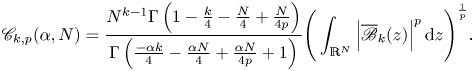 \[ \mathscr C_{k,p} (\alpha, N) = \frac{{N^{k-1}}\Gamma \left(1- \frac{k}{4}-\frac{N}{4}+\frac{N}{4p} \right)}{\Gamma \left( \frac{-\alpha k}{4}-\frac{\alpha N}{4}+\frac{\alpha N}{4p}+1 \right)} \Bigg( \int_{\mathbb{R}^{N}} \Big| \overline{\mathscr B}_k (z) \Big|^{p} \,{\textrm{d}}z \Bigg)^{\frac{1}{p}}. \]
Step 2. Verify the second inequality
The representation of  $\mathbb {K}_{2,\alpha } (t,x)$ and (2.4) together with Fubini's theorem imply
 \begin{align} \mathbb{K}_{2,\alpha} (t,x)&= \mathcal{F}^{{-}1} \Big(t^{\alpha-1} E_{\alpha,\alpha} ({-}t^{\alpha} |\xi|^{4})\Big)= t^{\alpha-1} \int_{\mathbb{R}^{N}} \,{\textrm{e}}^{{-}i <\xi, x>} \Big(E_{\alpha,\alpha} ({-}t^{\alpha} |\xi|^{4})\Big)\,{\textrm{d}}\xi\nonumber\\ &=t^{\alpha-1} \left({2\pi}\right)^{{-}N}\int_{\mathbb{R}^{N}} \,{\textrm{e}}^{i <\xi, x>} \Big(\int_0^{\infty} \alpha\zeta \mathcal{M}_\alpha (\zeta) \,{\textrm{e}}^{{-}t^{\alpha} \zeta |\xi|^{4}} \,{\textrm{d}}\zeta \Big)\,{\textrm{d}}\xi \nonumber\\ &= t^{\alpha-1} \left({2\pi}\right)^{{-}N}\int_0^{\infty} \alpha\zeta \mathcal{M}_\alpha (\zeta) \Bigg( \int_{\mathbb{R}^{N}} \,{\textrm{e}}^{i <\xi, x>}\,{\textrm{e}}^{{-}t^{\alpha} \zeta |\xi|^{4}}\,{\textrm{d}}\xi \Bigg) \,{\textrm{d}}\zeta. \end{align}
By setting  $\xi = \vartheta (t^{\alpha } \zeta )^{-\frac {1}{4}}$, we deduce
  ${\textrm {d}}\xi = (t^{\alpha } \zeta )^{-\frac {N}{4}} {\textrm {d}}\vartheta$ and
  $|\xi |^{4}= (t^{\alpha } \zeta )^{-1} |\vartheta |^{4}$. Using (2.14),
 \[ \mathbb{K}_{2,\alpha} (t,x)= \alpha t^{\alpha-1} \int_0^{\infty} \zeta (t^{\alpha} \zeta)^{-\frac{N}{4}} \mathcal{M}_\alpha (\zeta) \int_{\mathbb{R}^{N}} \,{\textrm{e}}^{i <\vartheta, x> t^{-\frac{\alpha}{4}}\eta^{-\frac{1}{4}}} \,{\textrm{e}}^{-|\vartheta|^{4}} d \vartheta \,{\textrm{d}}\zeta. \]
By a similar argument as in step 1,
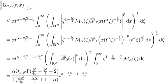 \begin{align*} &\Big\|\mathbb{K}_{2,\alpha} (t,x)\Big\|_{L^{p}}\\ &\quad \le \alpha t^{\alpha-\frac{\alpha N}{4}-1} \int_0^{\infty} \Bigg( \int_{\mathbb{R}^{N}} \Bigg| \zeta^{1-\frac{N}{4}} \mathcal{M}_\alpha (\zeta) \overline{\mathscr B}_0 (x (t^{\alpha} \zeta)^{-\frac{1}{4}} ) \Bigg| ^{p} \,{\textrm{d}}x \Bigg)^{\frac{1}{p}} \,{\textrm{d}}\zeta \\ &\quad = \alpha t^{\alpha-\frac{\alpha N}{4}-1} \int_0^{\infty} \Bigg( \int_{\mathbb{R}^{N}} \Big| \zeta^{1-\frac{N}{4}} \mathcal{M}_\alpha (\zeta) \overline{\mathscr B}_0 \left(x (t^{\alpha} \zeta)^{-\frac{1}{4}} \right) \Big| ^{p} (t^{\alpha} \zeta)^{\frac{N}{4}} \,{\textrm{d}}z\Bigg)^{\frac{1}{p}} \,{\textrm{d}}\zeta \\ &\quad = \alpha t^{\alpha-\frac{\alpha N}{4}-1+\frac{\alpha N}{4p}} \Bigg( \int_{\mathbb{R}^{N}} \Big| \overline{\mathscr B}_0 (z) \Big|^{p} \,{\textrm{d}}z\Bigg)^{\frac{1}{p}} \int_0^{\infty} \zeta^{1+\frac{N}{4p}-\frac{N}{4}} \mathcal{M}_\alpha (\zeta) \,{\textrm{d}}\zeta \\ &\quad = \frac{\alpha \Theta_{p,N} \Gamma(\frac{N}{4p}-\frac{N}{4}+2) }{\Gamma(\frac{\alpha N}{4p}-\frac{\alpha N}{4}+1+\alpha) } t^{\alpha-\frac{\alpha N}{4}-1+\frac{\alpha N}{4p}}. \end{align*}
Now, we estimate the derivative of the quantity  $\mathbb {K}_{2,\alpha }$. Let us recall the following formula
 \[ \mathbb{K}_{2,\alpha} (t,x) =t^{\alpha-1-\frac{\alpha N}{4}} \int_0^{\infty} \alpha \zeta^{1-\frac{N}{4}} \mathcal{M}_\alpha (\zeta) \overline{\mathscr B}_0 \big(xt^{-\frac{\alpha}{4}} \zeta^{-\frac{1}{4}} \big)\,{\textrm{d}}\zeta. \]
In view of the boundedness of  $D \mathbb {K}_{1,\alpha } (t,x)$, we have
 \begin{align} \big|D^{k} \mathbb{K}_{2,\alpha} (t,x)\big| \le t^{\alpha-1-\frac{\alpha N}{4}} \int_0^{\infty} \alpha \zeta^{1-\frac{N}{4}} \mathcal{M}_\alpha (\zeta) \big| D^{k} \overline{\mathscr B}_0 (x (t^{\alpha} \zeta )^{-\frac{1}{4}} ) \big|{\textrm{d}}\zeta. \end{align}
It follows from  $|\vartheta |^{k}{\le N^{k-1}}\sum _{j=1}^{N} |\vartheta _j|^{k}$ that
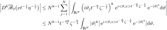 \begin{align} \Big| D^{k} \overline{\mathscr B}_0 \big(xt^{-\frac{1}{4}} \eta^{-\frac{1}{4}} \big) \Big| &\le{N^{k-1}} \sum_{j=1}^{N} \Bigg| \int_{\mathbb{R}^{N}} \left({i\vartheta_j t^{-\frac{\alpha}{4}} \zeta^{-\frac{1}{4}}}\right)^{k} \,{\textrm{e}}^{i <\vartheta,x> t^{-\frac{\alpha}{4}} \zeta^{-\frac{1}{4}}} \,{\textrm{e}}^{-|\vartheta|^{4}} {\textrm{d}}\vartheta \Bigg|\nonumber\\ &\le {N^{k-1}}t^{-\frac{\alpha k}{4}} \zeta^{-\frac{k}{4}} \int_{\mathbb{R}^{N}} |\vartheta|^{k} \big|\,{\textrm{e}}^{i <\vartheta,x> t^{-\frac{\alpha}{4}} \zeta^{-\frac{1}{4}}} \,{\textrm{e}}^{-|\vartheta|^{4}} \big| {\textrm{d}}\vartheta. \end{align}
By using substitution  $x (t^{\alpha } \zeta )^{-\frac {1}{4}} =z$, the second derivative with respect to
  $x$ of
  $\mathbb {K}_{2,\alpha } (t,x)$ is estimated by
 \begin{align*} &\Big\| D^{k} \mathbb{K}_{2,\alpha} (t,x) \Big\|_{L^{p}}= \Bigg( \int_{\mathbb{R}^{N}} \Big| D^{k} \mathbb{K}_{2,\alpha} (t,x) \Big|^{p} \,{\textrm{d}}x \Bigg)^{\frac{1}{p}}\\ &\quad\le {N^{k-1}} \Bigg( \int_{\mathbb{R}^{N}} \Bigg| t^{\alpha-1-\frac{\alpha N}{4}-\frac{\alpha k}{4}} \int_0^{\infty} \alpha \zeta^{1-\frac{N}{4}-\frac{k}{4}} \mathcal{M}_\alpha (\zeta) \int_{\mathbb{R}^{N}} |\vartheta|^{k} \Big|\\ &\qquad \times \exp\Big({i <\vartheta,x> t^{-\frac{1}{4}} \zeta^{-\frac{1}{4}}}\Big) \,{\textrm{e}}^{-|\vartheta|^{4}} \Big| {\textrm{d}}\vartheta \,{\textrm{d}}\zeta \Bigg|^{p} \,{\textrm{d}}x\Bigg)^{\frac{1}{p}} \\ &\quad={N^{k-1}} \Bigg( \int_{\mathbb{R}^{N}} \Bigg| t^{\alpha-1-\frac{\alpha N}{4}-\frac{\alpha k}{4}} \int_0^{\infty} \alpha \mathcal{M}_\alpha (\zeta) \zeta^{1-\frac{N}{4}-\frac{ k}{4}} \overline {\mathscr B}_k \big( z\big) \,{\textrm{d}}\zeta\Bigg|^{p} \,{\textrm{d}}x \Bigg)^{\frac{1}{p}} \\ &\quad \le{N^{k-1}} t^{\alpha-1-\frac{\alpha N}{4}-\frac{\alpha k}{4}} \Bigg( \int_{\mathbb{R}^{N}} \Big| \int_0^{\infty} \alpha \mathcal{M}_\alpha (\zeta) \zeta^{1-\frac{N}{4}-\frac{ k}{4}} \overline {\mathscr B}_k \big( z\big) \,{\textrm{d}}\zeta \Big|^{p} \,{\textrm{d}}x \Bigg)^{\frac{1}{p}}. \end{align*}
Applying Minkowski's inequality in integral form, we find that
 \begin{align} &\Big\| D^{k} \mathbb{K}_{2,\alpha} (t,x) \Big\|_{L^{p}} \notag\\ &\quad \le{N^{k-1}} t^{\alpha-1-\frac{\alpha N}{4}-\frac{\alpha k}{4}} \Bigg( \int_{\mathbb{R}^{N}} \Big| \int_0^{\infty} \alpha \mathcal{M}_\alpha (\zeta) \zeta^{1-\frac{N}{4}-\frac{ k}{4}} \overline {\mathscr B}_k \big( z\big) \,{\textrm{d}}\zeta \Big|^{p} \,{\textrm{d}}x \Bigg)^{\frac{1}{p}} \nonumber\\ &\quad \le{N^{k-1}} \alpha t^{\alpha-1-\frac{\alpha N}{4}-\frac{\alpha k}{4}} \int_0^{\infty} \Bigg( \int_{\mathbb{R}^{N}} \Big| \mathcal{M}_\alpha (\zeta) \zeta^{1-\frac{N}{4}-\frac{ k}{4}} \overline {\mathscr B}_k \big( z\big) \Big|^{p} (t^{\alpha} \zeta)^{\frac{N}{4}} \,{\textrm{d}}z\Bigg)^{\frac{1}{p}} \,{\textrm{d}}\zeta \nonumber\\ &\quad \le{N^{k-1}} \alpha t^{\alpha-\frac{\alpha N}{4}-1+\frac{\alpha N}{4p}-\frac{\alpha k}{4}} \int_0^{\infty} \zeta^{1-\frac{N}{4}+\frac{N}{4p}-\frac{ k}{4}} \mathcal{M}_\alpha (\zeta) \Bigg( \int_{\mathbb{R}^{N}} \Big| \overline{ \mathscr B}_k (z ) \Big| ^{p} \,{\textrm{d}}z\Bigg)^{\frac{1}{p}} \,{\textrm{d}}\zeta \nonumber\\ &\quad ={N^{k-1}}\alpha \Bigg( \int_{\mathbb{R}^{N}} \Big| \overline{\mathscr B}_k (z) \Big|^{p} \,{\textrm{d}}z\Bigg)^{\frac{1}{p}} t^{\alpha-\frac{\alpha N}{4}-1+\frac{\alpha N}{4p}-\frac{\alpha k}{4}} \int_0^{\infty} \zeta^{1-\frac{N}{4}+\frac{N}{4p}-\frac{ k}{4}} \mathcal{M}_\alpha (\zeta) \,{\textrm{d}}\zeta. \end{align}
Let us continue by computing the integral term on the right-hand side (RHS) of (2.4). Indeed, using lemma (5.2) and noting that  $2-\frac {N}{4}+\frac {N}{4p}-\frac { k}{4}>0$, we immediately derive
 \begin{equation} \int_0^{\infty} \zeta^{1-\frac{N}{4}+\frac{N}{4p}-\frac{ k}{4}} \mathcal{M}_\alpha (\zeta)\,{\textrm{d}}\zeta= \frac{\Gamma \left( 2-\frac{N}{4}+\frac{N}{4p}-\frac{ k}{4} \right)}{\Gamma \left( 1+\alpha-\frac{\alpha N}{4}+\frac{\alpha N}{4p}-\frac{ \alpha k}{4} \right)}. \end{equation}
Combining (2.17) and (2.18), we find that there exists  $\overline { \mathscr C_{k,p}} (\alpha , N)$ such that
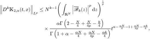 \begin{align*} \Big\| D^{k} \mathbb{K}_{2,\alpha} (t,x) \Big\|_{L^{p}} &\le {N^{k-1}}\Bigg( \int_{\mathbb{R}^{N}} \Big| \overline{\mathscr B}_k (z) \Big|^{p} \,{\textrm{d}}z \Bigg)^{\frac{1}{p}}\\ &\quad \times \frac{\alpha \Gamma \left( 2-\frac{N}{4}+\frac{N}{4p}-\frac{ k}{4} \right)}{\Gamma \left( 1+\alpha-\frac{\alpha N}{4}+\frac{\alpha N}{4p}-\frac{ \alpha k}{4} \right)} t^{\alpha-\frac{\alpha N}{4}-1+\frac{\alpha N}{4p}-\frac{\alpha k}{4}} .\end{align*}
We end the proof here.
Remark 2.3 Let us state some comments on the assumptions of the above lemma as follows.
(i) When
$p=1$ the assumption $k<4-N(1-\frac {1}{p})$ implies that we can take $k$ from the set $\{0,1,2,3\}$. In addition, when $p=1$ and $k=0$, from the facts that $\Theta _{1,N}=1,\ \frac {\alpha }{\Gamma (1+\alpha )}<\Gamma (2)=1$, we can bound $\mathscr C_{k,p}$ and $\overline { \mathscr C_{k,p}}$ by $1$.(ii) When
$k=0$, the assumption becomes $\frac {N}{4}(1-\frac {1}{p})<1$. This assumption is always satisfied whenever $N\le 4$. On the other hand, when $N\ge 5$, we need to consider the condition that $p<\frac {N}{N-4}$ further, if we want to apply this lemma.(iii) When
$k\ge 1$, we have a certain restriction on the hypothesis for $p$. For example, when $N=4$ the hypothesis $1\le p<\frac {N}{N-k}$ implies that $p\in \{1,2,3\}.$ In short, when using lemma 2.3, the larger $k$ and dimension $N$, the more restricted on the amount of $p.$


Remark 2.4 From [Reference Galaktionov and Pohozaev23, proposition 2.1], we can bound  $\Theta _{p,N}$ by a constant
  $\Theta _{N}$ independent of
  $p$. This fact will be needed when we set up some linear estimates.
2.2 Space setting
Definition 2.4 Assume that a function  $\Xi :\mathbb {R}^{+}\cup \{0\}\rightarrow \mathbb {R}^{+}\cup \{0\}$ is increasing convex, right continuous at
  $0$ and
 \[ \lim_{z\to\infty}\Xi(z)=\infty. \]
Then, we define the Orlicz space  $L^{\Xi }(\mathbb {R}^{N})$ in the following fashion
 \[ L^{\Xi}(\mathbb{R}^{N})=\left\{\varphi\in L_\textrm{loc}^{1}(\mathbb{R}^{N});\int_{\mathbb{R}^{N}}\Xi\left({\frac{|\varphi(x)|}{\kappa}}\right)\,{\textrm{d}}x<\infty,\text{ for some }\kappa>0\right\}. \]
Remark 2.5 The Orlicz space  $L^{\Xi }(\mathbb {R}^{N})$ mentioned above is a Banach space, endowed with the Luxemburg norm
 \[ \left\| {\varphi} \right\|_{\Xi}=\inf\left\{\kappa>0;\int_{\mathbb{R}^{N}}\Xi\left({\frac{|\varphi(x)|}{\kappa}}\right)\,{\textrm{d}}x\le 1\right\}. \]
Remark 2.6 Let  $1< p <\infty$, by choosing
  $\Xi (z)=z^{p}$, we can identify the space
  $L^{\Xi }(\mathbb {R}^{N})$ with the usual Lebesgue space
  ${L^{p}(\mathbb {R}^{N})}.$ For the sake of brevity, we set
 \[ \left\| {\cdot} \right\|_{L^{p}+L^{q}}:=\left\| {\cdot} \right\|_{{L^{p}(\mathbb{R}^{N})}\cap{L^{q}(\mathbb{R}^{N})}},\quad p,\ q\in[1;\infty]. \]
Definition 2.5 Let  $1\le p <\infty$, in the rest of this study, we use the symbol
  ${L^{\Xi }(\mathbb {R}^{N})}$ to indicate the Orlicz spaces with
  $\Xi (z)={\textrm {e}}^{|z|^{p}}-1$. We also denote
 \[ \left\| {\cdot} \right\|_{L^{q}+\Xi}:=\left\| {\cdot} \right\|_{{L^{q}(\mathbb{R}^{N})}\cap{L^{\Xi}(\mathbb{R}^{N})}},\quad q\in[1;\infty]. \]
Definition 2.6 Let  $1\le p<\infty$. We define the following subspace of
  ${L^{\Xi }(\mathbb {R}^{N})}$
 \[ L^{\Xi}_0(\mathbb{R}^{N})=\left\{\varphi\in L_\textrm{loc}^{1}(\mathbb{R}^{N});\int_{\mathbb{R}^{N}}\Xi\left({\frac{|\varphi(x)|}{\kappa}}\right)\,{\textrm{d}}x<\infty,\text{ for every }\kappa>0\right\}. \]
Remark 2.7 It can be shown from [Reference Ioku, Ruf and Terraneo25] that  ${L^{\Xi }_{0}(\mathbb {R}^{N})}=\overline {C_0^{\infty }(\mathbb {R}^{N})}^{{L^{\Xi }(\mathbb {R}^{N})}}.$
From the previous definitions, we can note that the Orlicz space is a generalization of the usual Lebesgue space. Let us introduce some of the useful embeddings between Orlicz spaces and Lebesgue spaces that we will need in our main results section.
Lemma 2.7 For every constants  $p,q$ satisfying
  $1\le p\le q<\infty$, the embedding
  ${L^{\Xi }(\mathbb {R}^{N})}\hookrightarrow {L^{q}(\mathbb {R}^{N})}$ holds. In addition,
 \begin{align} \left\| {\varphi} \right\|_{L^{q}}\le\left[{\Gamma\left({\frac{q}{p}+1}\right)}\right]^{\frac{1}{q}}\left\| {\varphi} \right\|_{\Xi}. \end{align}
Lemma 2.8 Given  $1\le q\le p$, we have
  ${L^{q}(\mathbb {R}^{N})}\cap L^{\infty }(\mathbb {R}^{N})\hookrightarrow {L^{\Xi }_{0}(\mathbb {R}^{N})}\subsetneq {L^{\Xi }(\mathbb {R}^{N})}$. In particular, for any
  $\varphi \in {L^{q}(\mathbb {R}^{N})}\cap L^{\infty }(\mathbb {R}^{N})$ the following bound holds
 \[ \left\| {\varphi} \right\|_{\Xi}\le(\log 2)^{\frac{-1}{p}}\left[{\left\| {\varphi} \right\|_{L^{q}}+\left\| {\varphi} \right\|_{L^{\infty}}}\right]. \]
Lemma 2.9 Let  $p\ge 1$ and
  $\alpha \in (0,1)$. Then, we can find constants
  $\mathscr {C}_{1,h},\mathscr {C}_{2,h},\mathscr {C}_{\Xi }$ such that the following results hold.
(i) Suppose that
$h\in [1,p]$ satisfies $h>N/4$, for any $\varphi \in {L^{h}(\mathbb {R}^{N})}$, we have
\begin{align*} \left\| {\mathbb{Z}_{1,\alpha}(t)\varphi} \right\|_{\Xi}&\le {\mathscr{C}_{1,h}}t^{\frac{-\alpha N}{4h}}\left[{\log\left({1+t^{\frac{-\alpha N}{4}}}\right)}\right]^{\frac{-1}{p}}\left\| {\varphi } \right\|_{L^{h}},\\ \left\| {\mathbb{Z}_{2,\alpha}(t)\varphi} \right\|_{\Xi}&\le {\mathscr{C}_{2,h}}t^{\frac{-\alpha N}{4q}}\left[{\log\left({1+t^{\frac{-\alpha N}{4}}}\right)}\right]^{\frac{-1}{p}}\left\| {\varphi } \right\|_{L^{h}}. \end{align*}(ii) For any
$\varphi \in {L^{\Xi }(\mathbb {R}^{N})},$ we have
\[ \left\| {\mathbb{Z}_{1,\alpha}(t)\varphi} \right\|_{\Xi}\le \left\| {\varphi } \right\|_{\Xi},\quad\left\| {\mathbb{Z}_{2,\alpha}(t)\varphi} \right\|_{\Xi}\le t^{\alpha-1}\left\| {\varphi } \right\|_{\Xi}. \]


Proof. Firstly, by using Young's convolution inequality, there exists a constant  $q\in [1,\infty ]$ such that
 \begin{equation} \left\| {\mathbb{Z}_{i,\alpha}(t)\varphi} \right\|_{L^{p}}\le\left\| {\mathbb{K}_{i,\alpha}(t)} \right\|_{L^{q}}\left\| {\varphi} \right\|_{L^{h}}. \end{equation}
Then, thanks to lemma 2.3, we have
 \begin{align*} \left\| {\mathbb{Z}_{1,\alpha}(t)\varphi} \right\|_{L^{p}}&\le \frac{\Theta_{N}\Gamma\left({1-\frac{ N}{4}\left({\frac{1}{h}-\frac{1}{p}}\right)}\right)}{\Gamma\left({1-\frac{ \alpha N}{4}\left({\frac{1}{h}-\frac{1}{p}}\right)}\right)}t^{\frac{- \alpha N}{4}\left({\frac{1}{h}-\frac{1}{p}}\right)}\left\| {\varphi} \right\|_{L^{h}},\\ \left\| {t^{1-\alpha}\mathbb{Z}_{2,\alpha}(t)\varphi} \right\|_{L^{p}}&=t^{1-\alpha}\left\| {\mathbb{Z}_{2,\alpha}(t)\varphi} \right\|_{L^{p}}\\ & \le \frac{\alpha \Theta_{N}\Gamma\left({2-\frac{ N}{4}\left({\frac{1}{h}-\frac{1}{p}}\right)}\right)}{\Gamma\left({2-\frac{ \alpha N}{4}\left({\frac{1}{h}-\frac{1}{p}}\right)}\right)}t^{\frac{-\alpha N}{4}\left({\frac{1}{h}-\frac{1}{p}}\right)}\left\| {\varphi} \right\|_{L^{h}}. \end{align*}
 We can show that the constants on the RHS of the above estimates can be bounded by two constants  $\mathscr {C}_{1,h},\mathscr {C}_{2,h}$ that are independent of
  $p$, respectively. In fact, by properties of the Gamma function when
  $0<\frac {N}{4}\left ({\frac {1}{h}-\frac {1}{p}}\right )<1<\frac {29}{20}$, we obtain
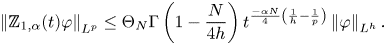 \[ \left\| {\mathbb{Z}_{1,\alpha}(t)\varphi} \right\|_{L^{p}}\le \Theta_{N}\Gamma\left({1-\frac{ N}{4h}}\right)t^{\frac{- \alpha N}{4}\left({\frac{1}{h}-\frac{1}{p}}\right)}\left\| {\varphi} \right\|_{L^{h}}. \]
On the other hand, the Gautschi inequality implies
 \[ \frac{\Gamma\left({2-\frac{N}{4}\left({\frac{1}{h}-\frac{1}{p}}\right)}\right)}{\Gamma\left({2-\frac{\alpha N}{4}\left({\frac{1}{h}-\frac{1}{p}}\right)}\right)}\le\left[{1-\frac{\alpha N}{4}\left({\frac{1}{h}-\frac{1}{p}}\right)}\right]^{\frac{(\alpha-1)N}{4}\left({\frac{1}{h}-\frac{1}{p}}\right)} \le\left({1-\frac{\alpha N}{4h}}\right)^{\frac{(\alpha-1)N}{4h}}. \]
It follows that
 \[ \left\| {t^{1-\alpha}\mathbb{Z}_{2,\alpha}(t)\varphi} \right\|_{L^{p}}\le \alpha\Theta_{N}\left({1-\frac{\alpha N}{4h}}\right)^{\frac{(\alpha-1)N}{4h}}t^{\frac{-\alpha N}{4}\left({\frac{1}{h}-\frac{1}{p}}\right)}\left\| {\varphi} \right\|_{L^{h}}. \]
We are now ready to verify our main statements. Because the techniques are the same, we will present only the proof for the second one,  $\mathbb {Z}_{2,\alpha }(t)\varphi$. We note that for
  $j\ge 1$
 \[ \left\| {t^{1-\alpha}\mathbb{Z}_{2,\alpha}(t)\varphi} \right\|_{L^{pj}}^{pj} \le \mathscr{C}_{2,h}^{pj}t^{\frac{-\alpha Npj}{4}\left({\frac{1}{h}-\frac{1}{pj}}\right)}\left\| {\varphi } \right\|_{L^{h}}^{pj}\le t^{\frac{\alpha N}{4}}\left[{\mathscr{C}_{2,h}t^{\frac{-\alpha N}{4h}}\left\| {\varphi } \right\|_{L^{h}}}\right]^{pj}. \]
Then, the Taylor expansion of the exponential leads us to
 \begin{align} \int_{\mathbb{R}^{N}}\left[{\exp\left({\frac{\left|t^{1-\alpha}\mathbb{Z}_{2,\alpha}(t)\varphi(x)\right|^{p}}{\kappa^{p}}}\right)-1}\right]\,{\textrm{d}}x &=\sum_{j=1}^{\infty}\frac{\left\| {t^{1-\alpha}\mathbb{Z}_{2,\alpha}(t)\varphi} \right\|_{L^{pj}}^{pj}}{j!\kappa^{pj}}\nonumber\\ &\le t^{\frac{\alpha N}{4}}\sum_{j=1}^{\infty}\frac{\left[{\mathscr{C}_{2,h}t^{\frac{-\alpha N}{4h}}\left\| {\varphi } \right\|_{L^{h}}}\right]^{pj}}{j!\kappa^{pj}} \nonumber\\ &=t^{\frac{\alpha N}{4}}\left[{\exp\left({\frac{\mathscr{C}_{2,h}t^{\frac{-\alpha N}{4h}}\left\| {\varphi } \right\|_{L^{h}}}{\kappa}}\right)^{p}-1}\right]. \end{align}
Next, assume that the RHS of the above estimate is less than or equal 1. Then, we can easily find that
 \[ \mathscr{C}_{2,h}t^{\frac{-\alpha N}{4h}}\left[{\log\left({1+t^{\frac{-\alpha N}{4}}}\right)}\right]^{\frac{-1}{p}}\left\| {\varphi } \right\|_{L^{h}}\le\kappa. \]
In view of (2.21), if we set
 \begin{align*} A&:=\left\{\kappa>0;\int_{\mathbb{R}^{N}}\left[{\exp\left({\frac{\left|\mathbb{Z}_{2,\alpha}(t)\varphi(x)\right|^{p}}{\kappa^{p}}}\right)-1}\right]\,{\textrm{d}}x\le 1\right\},\\ B&:=\left\{\kappa>0;\mathscr{C}_{2,h}t^{\frac{-\alpha N}{4h}}\left[{\log\left({1+t^{\frac{-\alpha N}{4}}}\right)}\right]^{\frac{-1}{p}}\left\| {\varphi } \right\|_{L^{h}}\le\kappa\right\}, \end{align*}
the cover result  $B\subset A$ holds. This implies that
 \[ \inf A\le\inf B=\mathscr{C}_{2,h}t^{\frac{-\alpha N}{4h}}\left[{\log\left({1+t^{\frac{-\alpha N}{4}}}\right)}\right]^{\frac{-1}{p}}\left\| {\varphi} \right\|_{L^{h}}. \]
We obtain the first results of this lemma. To prove the remaining result, we only need to modify slightly inequality (2.21) in the following way
 \begin{align*} \int_{\mathbb{R}^{N}}\left[{\exp\left({\frac{\left|t^{1-\alpha}\mathbb{Z}_{2,\alpha}(t)\varphi(x)\right|^{p}}{\kappa^{p}}}\right)-1}\right]\,{\textrm{d}}x&=\sum_{j=1}^{\infty}\frac{\left\| {t^{1-\alpha}\mathbb{Z}_{2,\alpha}(t)\varphi} \right\|_{L^{pj}(\mathbb{R}^{N})}^{pj}}{j!\kappa^{pj}}\\ &\le \sum_{j=1}^{\infty}\frac{\left\| {\varphi } \right\|_{L^{pj}(\mathbb{R}^{N})}^{pj}}{j!\kappa^{pj}}=\exp\left({\frac{\left\| {\varphi } \right\|_{L^{p}}}{\kappa}}\right)^{p}-1. \end{align*}
Then, our statements follow.
Proposition 2.1 Assume that  $\varphi \in {L^{\Xi }_{0}(\mathbb {R}^{N})}$. Then, we have
 \[ \mathbb{Z}_{1,\alpha}(t)\varphi\in C\left({[0,T];{L^{\Xi}_{0}(\mathbb{R}^{N})}}\right). \]
Proof. Since  $\varphi \in {L^{\Xi }_{0}(\mathbb {R}^{N})}$, there exists a sequence
  $\{\varphi _n\}_{n\in \mathbb {N}}\subset C_{0}^{\infty }(\mathbb {R}^{N})$ such that
  $\varphi _n$ converges to
  $\varphi$ with respect to
  ${L^{\Xi }(\mathbb {R}^{N})}$ norm. This implies that, for any
  $t>0$,
  $\mathbb {Z}_{1,\alpha }(t)\varphi _n$ will converge to
  $\mathbb {Z}_{1,\alpha }(t)\varphi .$ Indeed, by applying lemma 2.9, we have
 \[ \left\| {\mathbb{Z}_{1,\alpha}(t)\varphi_n-\mathbb{Z}_{1,\alpha}(t)\varphi} \right\|_{\Xi}\le\left\| {\varphi_n-\varphi} \right\|_{\Xi}\xrightarrow{n\rightarrow\infty}0. \]
By taking two number  $t_1,t_2>0$, the triangle inequality implies
 \begin{align*} &\left\| {\mathbb{Z}_{1,\alpha}(t_2)\varphi-\mathbb{Z}_{1,\alpha}(t_1)\varphi} \right\|_{\Xi}\\ &\quad\le\left\| {\mathbb{Z}_{1,\alpha}(t_2)\varphi_n-\mathbb{Z}_{1,\alpha}(t_2)\varphi} \right\|_{\Xi}+\left\| {\mathbb{Z}_{1,\alpha}(t_1)\varphi_n-\mathbb{Z}_{1,\alpha}(t_1)\varphi} \right\|_{\Xi}\\ &\qquad+\left\| {\mathbb{Z}_{1,\alpha}(t_2)\varphi_n-\mathbb{Z}_{1,\alpha}(t_1)\varphi_n} \right\|_{\Xi}. \end{align*}
Combining lemma 2.9, the definition of  ${L^{\Xi }_{0}(\mathbb {R}^{N})}$ and the application of theorem 2.2 for
  ${L^{p}(\mathbb {R}^{N})}$ and
  $C_0(\mathbb {R}^{N})$
 \[ \begin{cases} \lim_{t_2\to t_1}\left\| {\mathbb{Z}_{1,\alpha}(t_2)\varphi_n-\mathbb{Z}_{1,\alpha}(t_1)\varphi_n} \right\|_{L^{p}}=0, & \varphi_n\in C_{0}^{\infty}(\mathbb{R}^{N}),\\ \lim_{t_2\to t_1}\left\| {\mathbb{Z}_{1,\alpha}(t_2)\varphi_n-\mathbb{Z}_{1,\alpha}(t_1)\varphi_n} \right\|_{L^{\infty}}=0, & \varphi_n\in C_{0}^{\infty}(\mathbb{R}^{N}), \end{cases} \]
and
 \[ \begin{cases} \lim_{n\to\infty}\left\| {\mathbb{Z}_{1,\alpha}(t_1)\varphi_n-\mathbb{Z}_{1,\alpha}(t_1)\varphi} \right\|_{\Xi}=0,\\ \lim_{n\to\infty}\left\| {\mathbb{Z}_{1,\alpha}(t_2)\varphi_n-\mathbb{Z}_{1,\alpha}(t_2)\varphi} \right\|_{\Xi}=0. \end{cases} \]
Consequently, by an appropriate choice of  $n$, the desired conclusion of this proposition can be drawn easily.
3. Time-fractional biharmonic equation with exponential nonlinearity
In this section, we investigate the IVP for the time-fractional biharmonic equation with exponential nonlinearity
 \begin{equation} \begin{cases} \partial^{\alpha}_{0|t}{u}(t,x)+\Delta^{2}{u}(t,x)=G(u(t,x)),\quad & \mbox{in}\quad\mathbb{R}^{+}\times\mathbb{R}^{N},\\ {u}(0,x)={u}_0(x), & \mbox{in} \quad \mathbb{R}^{N}, \end{cases} \end{equation}
with the following assumptions of the initial function:
Assumption 1 The initial function  ${u}_0$ belongs to
  ${L^{p}(\mathbb {R}^{N})}\cap {C_0(\mathbb {R}^{N})}$.
Assumption 2 The initial function  ${u}_0$ belongs to
  ${L^{\Xi }(\mathbb {R}^{N})}$ or
  ${L^{\Xi }_{0}(\mathbb {R}^{N})}$.
3.1 Unique existence of mild solution under the first assumption for the initial function
In this section, we investigate problem (P1) with the assumption that  $u_0$ belongs to the space
  ${L^{p}(\mathbb {R}^{N})}\cap {C_0(\mathbb {R}^{N})}$.
Theorem 3.1 Assume that  ${u}_0\in {L^{\Xi }(\mathbb {R}^{N})}\cap {C_0(\mathbb {R}^{N})}$. Then, there exists a unique solution of problem (P1) that belongs to
  $C\left ({(0,T];{L^{\Xi }(\mathbb {R}^{N})}\cap {C_0(\mathbb {R}^{N})}}\right )$.
Proof. The proof is begun by fixing a constant  $\Im >0$ and choosing a small time
  $T<\sqrt [\alpha ]{\alpha \Im _1^{-1}}$, where
  $\Im _1$ is defined in (3.7). Next, we consider the following space
 \[ \mathbf{A}:=\left\{u\in C\left({(0,T];{L^{\Xi}(\mathbb{R}^{N})}\cap{C_0(\mathbb{R}^{N})}}\right);\sup_{t\in(0,T]}\left\| {u(t)-\mathbb{Z}_{1,\alpha}(t){u}_{0}} \right\|_{L^{\infty}+\Xi}\le\Im \right\}, \]
and the operator  $\mathscr F:\mathbf {A}\rightarrow \mathbf {A}$ given by
 \begin{equation} \mathscr{F}u(t)=\mathbb{Z}_{1,\alpha}(t)u_{0}+\int_{0}^{t}\mathbb{Z}_{2,\alpha}(t-\tau)G(u(\tau))\,{\textrm{d}} \tau. \end{equation}
By Young's convolution inequality and lemma 2.3, we have
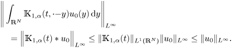 \begin{align*} &\Bigg\|\int_{\mathbb{R}^{N}} \mathbb{K}_{1,\alpha} (t,\cdot{-}y) u_0(y)\,{\textrm{d}}y\Bigg\|_{L^{\infty}}\\ &\quad =\Big\| \mathbb{K}_{1,\alpha} (t) * u_0 \Big\|_{L^{\infty}}\le \| \mathbb{K}_{1,\alpha} (t) \|_{L^{1}(\mathbb{R}^{N})} \| u_0 \|_{L^{\infty}} \le \|u_0 \|_{L^{\infty}}. \end{align*}
Then, for every  $u\in \mathbf {A}$, the following estimate holds
 \begin{align} \left\| {u(t)} \right\|_{L^{\infty}+\Xi}&\le\left\| {\mathbb{Z}_{1,\alpha}(t){u}_{0}} \right\|_{L^{\infty}+\Xi}+\left\| {u(t)-\mathbb{Z}_{1,\alpha}(t){u}_{0}} \right\|_{L^{\infty}+\Xi}\nonumber\\ &\le 2(\log 2)^{\frac{-1}{p}}\left\| {{u}_{0}} \right\|_{L^{\infty}+\Xi}+\Im=:\Im_0. \end{align}
Our main goal is to prove that the integral equation (3.1) has a unique solution by the fixed point argument. To this end, we present the following two steps.
Step 1. From (1.2), for any  $u\in \mathbb {A}$ and
  $t>0$, we deduce
 \begin{equation} \begin{cases} \left\| {G(u(t))} \right\|_{L^{\infty}}\le L\left\| {u(t)} \right\|^{m}_{L^{\infty}}\,{\textrm{e}}^{\kappa\left\| {u(t)} \right\|^{p}_{L^{\infty}}}\le L\Im_0^{m}\,{\textrm{e}}^{\kappa\Im_0^{p}},\\ \left\| {G(u(t))} \right\|_{L^{p}}\le L\left\| {u(t)} \right\|^{m}_{L^{mp}}\,{\textrm{e}}^{\kappa\left\| {u(t)} \right\|^{p}_{L^{\infty}}}\le L\Im_0^{m}\,{\textrm{e}}^{\kappa\Im_0^{p}}\left({\Gamma(m+1)}\right)^{\frac{1}{p}}, \end{cases} \end{equation}
where we have used lemma 2.7 to achieve the second inequality. It follows that
 \begin{align*} \left\| {G(u(t))} \right\|_{L^{\infty}+\Xi}&\le(\log 2)^{\frac{-1}{p}}\left\| {{G}(u(t))} \right\|_{L^{p}+L^{\infty}}+\left\| {{G}(u(t))} \right\|_{L^{\infty}}\\ &\le L\left({2+\left({\Gamma(m+1)}\right)^{\frac{1}{p}}}\right)\Im_0^{m}(\log 2)^{\frac{-1}{p}}\,{\textrm{e}}^{\kappa\Im_0^{p}}. \end{align*}
In addition, by using lemma 2.8 and applying theorem 2.2 with respect to the spaces  ${L^{p}(\mathbb {R}^{N})},C_0(\mathbb {R}^{N})$, for any
  $\tau ,t\in (0,T],$ we deduce
 \begin{equation} t^{1-\alpha}\mathbb{Z}_{2,\alpha}(t)G(u(\tau))\in C\left({(0,T];{L^{\Xi}(\mathbb{R}^{N})}\cap{C_0(\mathbb{R}^{N})}}\right). \end{equation}
Next, by taking a positive number  $h$ and
  $r\in \{t,t+h\}$, for any
  $t\ge \xi$, we obtain
 \begin{align*} &(t+h-\tau)^{\alpha-1}\left\| {(r-\tau)^{1-\alpha}\mathbb{Z}_{2,\alpha}(r-\tau)G(u(\tau))} \right\|_{L^{\infty}+\Xi}\\ &\quad \le(t-\tau)^{\alpha-1}\left\| { G(u(\tau))} \right\|_{L^{\infty}+\Xi} \le C(t-\tau)^{\alpha-1}. \end{align*}
Then, applying the Lebesgue dominated convergence theorem,
 \begin{align} \lim_{h\to 0}\left\| {\int_{0}^{t}(t+h-\xi)^{\alpha-1}\left[{\frac{\mathbb{Z}_{2,\alpha}(t+h-\tau)}{(t+h-\tau)^{\alpha-1}}-\frac{\mathbb{Z}_{2,\alpha}(t-\tau)}{(t-\tau)^{\alpha-1}}}\right]G(u(\tau))\,{\textrm{d}} \tau} \right\|_{L^{\infty}+\Xi}=0. \end{align}
On the other hand, using the fact that  $\lim _{h\to 0}\left |(t+h)^{\alpha }-h^{\alpha }-t^{\alpha }\right |=0$ and (3.4), we further find that
 \begin{align} \lim_{h\to 0}\left\| {\int_{0}^{t}\left[{(t+h-\xi)^{\alpha-1}-(t-\xi)^{\alpha-1}}\right]\frac{\mathbb{Z}_{2,\alpha}(t+h-\tau)}{(t+h-\tau)^{\alpha-1}}G(u(\tau))\,{\textrm{d}} \tau} \right\|_{L^{\infty}+\Xi}=0. \end{align}
For the purpose of proving that the integral term on the RHS of (3.1) is continuous on  $(0,T]$, we also need the upcoming fact
 \[ \int_{t}^{t+h}\left\| {\mathbb{Z}_{2,\alpha}(t+h-\tau)G(u(\tau))\,{\textrm{d}} \tau} \right\|_{L^{\infty}+\Xi}\,{\textrm{d}} \tau\le Ch^{\alpha}\xrightarrow{h\rightarrow 0}0. \]
Taking into consideration the above limit results and applying theorem 2.2 to  ${u}_{0}\in {L^{p}(\mathbb {R}^{N})}\cap {C_0(\mathbb {R}^{N})}$, we can claim that
  $\mathscr {F}u(t)$ is a continuous mapping on
  $(0,T].$
Step 2. By using the Hölder inequality, for a constant  $\aleph \in [1,\infty )$ and
  $u_1,u_2\in \mathbf {A}$, we have
 \begin{align*} &\left\| {G(u_1(\tau))-G(u_2(\tau))} \right\|_{L^{p}}\\ &\quad \le L\left[{\sum_{j=1,2}\left\| {|u_j(\tau)|^{m-1}\,{\textrm{e}}^{\kappa|u_j(\tau)|^{p}}} \right\|_{L^{\frac{\aleph p}{\aleph-1}}}}\right]\left\| {u_1(\tau)-u_2(\tau)} \right\|_{L^{\aleph p}}. \end{align*}
Since the embedding  ${L^{\Xi }(\mathbb {R}^{N})}\hookrightarrow {L^{q}(\mathbb {R}^{N})}$ holds for any
  $q\in [p,\infty )$, and
  $u_j(\tau )\in {C_0(\mathbb {R}^{N})} ( j=1,2)$, the above inequality becomes
 \begin{align*} \left\| {G(u_1(\tau))-G(u_2(\tau))} \right\|_{L^{p}}&\le 2L\left({\Gamma(\aleph+1)}\right)^{\frac{1}{\aleph p}}\left({\Gamma\left({\frac{\aleph(m-1)}{\aleph-1}+1}\right)}\right)^{\frac{\aleph-1}{\aleph p}}\\ &\quad \times \Im_0^{m-1}\,{\textrm{e}}^{\kappa\Im_0^{p}}\left\| {u_1(\tau)-u_2(\tau)} \right\|_{\Xi}. \end{align*}
On the other hand, it is a simple matter to check that
 \begin{align*} \left\| {G(u_1(\tau))-G(u_2(\tau))} \right\|_{L^{\infty}}&\le L\left[{\sum_{j=1,2}\|u_j(\tau)\|_{L^{\infty}}^{m-1}\,{\textrm{e}}^{\kappa\|u_j(\tau)\|_{L^{\infty}}^{p}}}\right]\left\| {u_1(\tau)-u_2(\tau)} \right\|_{L^{\infty}}\\ &\le 2L \Im_0 ^{m-1}\,{\textrm{e}}^{\kappa \Im_0 ^{p}}\left\| {u_1(\tau)-u_2(\tau)} \right\|_{L^{\infty}}. \end{align*}
The two above results help us to deduce
 \begin{align} &\left\| {G(u_1(\tau))-G(u_2(\tau))} \right\|_{L^{\infty}+\Xi}\nonumber\\ &\quad\le 2L\left[{2+\left({\Gamma(\aleph+1)}\right)^{\frac{1}{\aleph p}}\left({\Gamma\left({\frac{\aleph(m-1)}{\aleph-1}+1}\right)}\right)^{\frac{\aleph-1}{\aleph p}}}\right]\notag\\ &\quad \times (\log 2)^{\frac{-1}{p}} \Im_0 ^{m-1}\,{\textrm{e}}^{\kappa \Im_0 ^{p}}\left\| {u_1(\tau)-u_2(\tau)} \right\|_{L^{\infty}+\Xi}\nonumber\nonumber\\ &\quad=:\Im_1\left\| {u_1(\tau)-u_2(\tau)} \right\|_{L^{\infty}+\Xi}. \end{align}
Also, lemma 2.3 shows us that
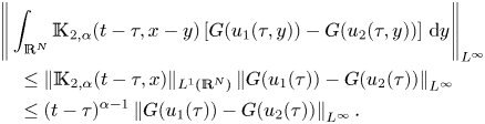 \begin{align*} &\Bigg\|\int_{\mathbb{R}^{N}} \mathbb{K}_{2,\alpha} (t-\tau,x-y) \left[{G(u_1(\tau,y))-G(u_2(\tau,y))}\right]\,{\textrm{d}}y\Bigg\|_{L^{\infty}} \\ &\quad\le \|\mathbb{K}_{2,\alpha} (t-\tau,x) \|_{L^{1}(\mathbb{R}^{N})}\left\| {G(u_1(\tau))-G(u_2(\tau))} \right\|_{L^{\infty}}\\ &\quad\le(t-\tau)^{\alpha-1}\left\| {G(u_1(\tau))-G(u_2(\tau))} \right\|_{L^{\infty}}. \end{align*}
From this result and lemma 2.9, we find that
 \begin{align*} \left\| {\mathscr{F}u_1(t)-\mathscr{F}u_2(t)} \right\|_{L^{\infty}+\Xi}&\le\int_{0}^{t}\left\| {\mathbb{Z}_{2,\alpha}(t-\tau)\left[{G(u_1(\tau))-G(u_2(\tau))}\right]} \right\|_{L^{\infty}+\Xi}\,{\textrm{d}} \tau\\ &\le\int_{0}^{t}(t-\tau)^{\alpha-1}\left\| {G(u_1(\tau))-G(u_2(\tau))} \right\|_{L^{\infty}+\Xi}\,{\textrm{d}} \tau \\ &\le \frac{T^{\alpha}\Im_1}{\alpha}\sup_{t \in(0, T]}\left\| {u_1(t)-u_2(t)} \right\|_{L^{\infty}+\Xi}. \end{align*}
By choosing  $u_2\equiv 0$ and
  $u_1\in \mathbf {A}$ in step 2, we derive
 \[ \sup_{t \in(0, T]}\left\| {\mathscr{F}u_1(t)-\mathbb{Z}_{1,\alpha}(t){u}_{0}} \right\|_{L^{\infty}+\Xi}\le\frac{T^{\alpha}\Im_1}{\alpha}\sup_{t \in(0, T]}\left\| {u_1(t)} \right\|_{L^{\infty}+\Xi}\le\Im. \]
This result along with step 1 show that  $\mathscr {F}$ is invariant on
  $\mathbf {A}$. Furthermore, it is obvious that
  $\mathbf {A}$ is a complete metric space with the metric
 \[ {\textrm{d}}(u,v):=\sup_{t \in(0, T]}\left\| {u(t)-v(t)} \right\|_{L^{\infty}+\Xi}. \]
 Therefore, the Banach principle argument can be applied to conclude that  $\mathscr {F}$ has a unique fixed point, which means that there exists a unique solution of the problem (P1) belonging to
  $\mathbf {A}$.
Lemma 3.2 Let  ${u}:(0,T]\rightarrow {L^{\Xi }(\mathbb {R}^{N})}\cap {C_0(\mathbb {R}^{N})}$ be the unique mild solution of problem (P1). Then there exists a unique continuous extension
  ${u}^{*}$ of
  $u$ on
  $(0,T+h],$ for some
  $h>0.$
Proof. The main idea of the proof is to show that there exists a unique solution of (P1) which belongs to the space
 \[ \mathbf{B}=\left\{ {w\in C\left({(0,T+h];{L^{\Xi}(\mathbb{R}^{N})}\cap{C_0(\mathbb{R}^{N})}}\right)\Biggl|\begin{array}{c} w(t)=u(t),\forall t\in(0,T]\\ \sup_{t \in[ T,T+h]}\left\| {w(t)-{u}(T)} \right\|_{L^{\infty}+\Xi}\le\Im \end{array}} \right\}, \]
 where  $\Im ,h>0$ will be chosen later. To this end, let us consider the function
  $\mathscr {J}:\mathbf {B}\rightarrow \mathbf {B},$ satisfying
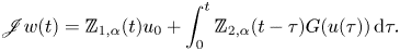 \[ \mathscr{J}w(t)=\mathbb{Z}_{1,\alpha}(t)u_{0}+\int_{0}^{t}\mathbb{Z}_{2,\alpha}(t-\tau)G(u(\tau))\,{\textrm{d}} \tau. \]
It is easily seen that for any  $t\in (0,T]$,
  $\mathscr {J}(w(t))=\mathscr {J}({u}(t))={u}(t)$. The continuity result of
  $\mathscr {J}$ on
  $(0,T+h]$ can be drawn by the same arguments as in theorem 3.1. Our remaining part of proving the well definition of
  $\mathscr {J}$ is to find that if
  $w\in \mathbf {B}$,
  $\sup _{t \in [ T,T+h]}\left \| {\mathscr {J}(w(t))-{u}(T)} \right \|_{L^{\infty }+\Xi }\le \Im$. Indeed, for any
  $t\in [T,T+h],$ we have
 \begin{align*} \left\| {\mathscr{J}(w(t))-{u}(T)} \right\|_{L^{\infty}+\Xi}&\le\underbrace{\left\| {\mathbb{Z}_{1,\alpha}(t){u}_{0}-\mathbb{Z}_{1,\alpha}(T){u}_{0}} \right\|_{L^{\infty}+\Xi}}_{(I)}\\ &\quad +\underbrace{\int_{T}^{t}\left\| {\mathbb{Z}_{2,\alpha}(t-\tau)G(u(\tau))} \right\|_{L^{\infty}+\Xi}\,{\textrm{d}} \tau}_{(II)}\\ &\quad+\underbrace{\int_{0}^{T}\Big\| \left[{\mathbb{Z}_{2,\alpha}(t-\tau)-\mathbb{Z}_{2,\alpha}(T-\tau)}\right]G(u(\tau)) \Big\|_{L^{\infty}+\Xi}\,{\textrm{d}} \tau}_{(III)}. \end{align*}
• Choosing a sufficiently small
$h_1$ and using theorem 2.2, lemma 2.8, for every $t\in [T,T+h_1],$ we can find that $(I)\le \frac {\Im }{3}$.• Choosing a sufficiently small
$h_2$, for every $t\in [T,T+h_2],$ we obtain
\begin{align*} (II)&\le \frac{L\left({2+\left({\Gamma(m+1)}\right)^{\frac{1}{p}}}\right)\left({\left\| {{u}(T)} \right\|_{L^{\infty}+\Xi}+\Im}\right)^{m}}{(\log 2)^{\frac{1}{p}}\,{\textrm{e}}^{-\kappa\left({\left\| {{u}(T)} \right\|_{L^{\infty}+\Xi}+\Im}\right)^{p}}} \int_{T}^{T+h_2}(t-\tau)^{\alpha-1}\,{\textrm{d}} \tau \\ &\le C\left[{(t-T)^{\alpha}-(t-T-h_2)^{\alpha}}\right]\le\frac{\Im}{3}. \end{align*}• Choosing a sufficiently small
$h_3$ and repeating the arguments for (3.5), (3.6), we can also find that
\[ (III)\le\frac{\Im}{3},\quad\text{for every}\ t\in[T,T+h_3]. \]


Additionally,  $\mathscr {J}$ is a contraction mapping on
  $\mathbf {B}$ if
  $h=h_4$ is small enough. In fact, for
  $u_1,u_2\in \mathbf {B},$ we have
 \begin{align*} &\left\| {\mathscr{J}u_1(t)-\mathscr{J}u_2(t)} \right\|_{L^{\infty}+\Xi}\le\int_{T}^{t}(t-\tau)^{\alpha-1}\left\| {G(u_1(\tau))-G(u_2(\tau))} \right\|_{L^{\infty}+\Xi}\,{\textrm{d}}\tau\\ &\quad \le\frac{2L \left[{2+\left({\Gamma(\aleph+1)}\right)^{\frac{1}{\aleph p}}\left({\Gamma\left({\frac{\aleph(m-1)}{\aleph-1}+1}\right)}\right)^{\frac{\aleph-1}{\aleph p}}}\right]}{\alpha h^{-\alpha}_4(\log 2)^{\frac{1}{p}}\left({\left\| {{u}(T)} \right\|+\Im}\right)^{1-m}\,{\textrm{e}}^{-\kappa\left({\left\| {{u}(T)} \right\|+\Im}\right)^{p}}}\sup_{t\in[T,T+h]}\left\| {u_1(t)-u_2(t)} \right\|_{L^{\infty}+\Xi}\\ &\quad \le\mathcal{L}\sup_{t \in[T,T+h]}\left\| {u_1(t)-u_2(t)} \right\|_{L^{\infty}+\Xi}. \end{align*}
Thanks to an appropriate choice of  $h_4$,
  $\mathcal {L}$ can be proved to be less than 1.
By setting  $h=\min \{h_1,h_2,h_3,h_4\}$, we can now apply the Banach principle arguments to declare that the solution to problem (P1) has been extended to some larger interval.
Theorem 3.3 Let  $T_{\max }$ be the supremum of the set of all
  $T>0$ such that problem (P1) has a unique local solution on
  $(0,T].$ Assume that
  $G$ satisfies (1.2) and
  ${u}_0$ belongs to
  ${L^{p}(\mathbb {R}^{N})}\cap {C_0(\mathbb {R}^{N})}$. Then, we can conclude that
  $T_{\max }=\infty$ or
  $T_{\max }<\infty$ and
  $\limsup _{t\to T_{\max }^{-}}\left \| {{u}(t)} \right \|_{L^{\infty }+\Xi }=\infty$.
Proof. Arguing by contradiction, we assume that  $T_{\max }<\infty$ and there exist a positive constant
  $\Im <\infty$ such that
 \begin{equation} \left\| {{u}(t)} \right\|_{L^{\infty}+\Xi}\le \Im. \end{equation}
Let  $\{t_j\}_{j\in \mathbb {N}}\subset (0,T_{\max })$ satisfy
  $t_j\xrightarrow {j\rightarrow \infty }T_{\max }$. Our goal is to show that
  $\{{u}(t_j)\}_{j\in \mathbb {N}}$ is a Cauchy sequence. To this end, let us take
  $t_a,t_b\in \{t_j\}_{j\in \mathbb {N}},$ without loss of generality, we suppose that
  $t_a< t_b$. Then, we have
 \begin{align*} \left\| {{u}(t_b)-{u}(t_a)} \right\|_{L^{\infty}+\Xi}&\le\left\| {\mathbb{Z}_{1,\alpha}(t_b){u}_{0}-\mathbb{Z}_{1,\alpha}(t_a){u}_{0}} \right\|_{L^{\infty}+\Xi}\\ &\quad+\int_{t_a}^{t_b}\left\| {\mathbb{Z}_{2,\alpha}(T_{\max}-\tau)G({u}(\tau))} \right\|_{L^{\infty}+\Xi}\,{\textrm{d}} \tau\\ &\quad+\int_{0}^{t_a}\Big\| \left[{\mathbb{Z}_{2,\alpha}(T_{\max}-\tau)-\mathbb{Z}_{2,\alpha}(t_a-\tau)}\right]G({u}(\tau)) \Big\|_{L^{\infty}+\Xi}\,{\textrm{d}} \tau\\ &\quad+\int_{0}^{t_b}\Big\| \left[{\mathbb{Z}_{2,\alpha}(t_b-\tau)-\mathbb{Z}_{2,\alpha}(T_{\max}-\tau)}\right]G({u}(\tau)) \Big\|_{L^{\infty}+\Xi}\,{\textrm{d}} \tau. \end{align*}
Given  $\varepsilon >0$, let us consider some large enough constants
  $j_1,j_2,j_3$ defined through the following steps.
Step 1. Thanks to the property of  $\mathbb {Z}_{1,\alpha }(t)$, we can choose a sufficiently large
  $j_1$ such that
 \[ \left\| {\mathbb{Z}_{1,\alpha}(t_b){u}_{0}-\mathbb{Z}_{1,\alpha}(t_a){u}_{0}} \right\|_{L^{\infty}+\Xi}<\frac{\varepsilon}{4},\quad\text{for any}\ a,b\ge j_1. \]
Step 2. For the sake of simplicity, let us set
 \[ \Im^{*}=L(\log 2)^{\frac{-1}{p}}\left({2+\left({\Gamma(m+1)}\right)^{\frac{1}{mp}}}\right)\Im^{m}\,{\textrm{e}}^{-\kappa \Im^{p}}. \]
and choose a large  $j_2$ such that
 \[ |t_j-T_{\max}|<\frac{\varepsilon\alpha}{8\Im^{*}},\quad\text{for any }j\ge j_2. \]
Then, similar to the proof of theorem 3.1, it is easily seen that
 \begin{align*} \int_{t_a}^{t_b}\left\| {\mathbb{Z}_{2,\alpha}(T_{\max}-\tau)G({u}(\tau))} \right\|_{L^{\infty}+\Xi}\,{\textrm{d}} \tau &\le\int_{t_a}^{t_b}(T_{\max}-\tau)^{\alpha-1}\left\| {G(u(\tau))} \right\|_{L^{\infty}+\Xi}\,{\textrm{d}} \tau\\ &\le\Im^{*}\alpha^{{-}1}\left({|t_b\,{-}\,T_{\max} |^{\alpha}+|t_a\,{-}\,T_{\max} |^{\alpha}}\right)<\frac{\varepsilon}{4}. \end{align*}
Step 3. The Lebesgue dominated convergence theorem helps us to find a sufficiently large  $j_3$ such that, for any
  $j\ge j_3$,
 \[ \int_{0}^{t_j}\left\| \left[{\mathbb{Z}_{2,\alpha}(T_{\max}-\tau)-\mathbb{Z}_{2,\alpha}(t_j-\tau)}\right]G({u}(\tau)) \right\|_{L^{\infty}+\Xi}\,{\textrm{d}} \tau<\frac{\varepsilon}{4}. \]
Now choosing  $j_0=\max \{j_1,j_2,j_3\}$ yields that
 \[ \left\| {{u}(t_a)-{u}(t_b)} \right\|_{L^{\infty}+\Xi}\le\varepsilon,\quad\text{for every }a,b\ge j_0. \]
Then, there exists a limit of the Cauchy sequence  $\{{u}(t_j)\}_{j\in \mathbb {N}}$ in
  ${L^{\Xi }(\mathbb {R}^{N})}\cap {C_0(\mathbb {R}^{N})}$ as
  $j$ tends to infinity denoted by
  ${u}^{*}$. Hence, we can check that
 \begin{align*} &\left\| {\int_{0}^{t_j}\mathbb{Z}_{2,\alpha}(t_j-\tau)G({u}(\tau))\,{\textrm{d}} \tau-\int_{0}^{T_{\max}}\mathbb{Z}_{2,\alpha}(T_{\max}-\tau)G({u}(\tau))\,{\textrm{d}} \tau} \right\|_{L^{\infty}+\Xi}\\ &\quad\le\int_{0}^{t_j}\left\| \left[{\mathbb{Z}_{2,\alpha}(t_j-\tau)-\mathbb{Z}_{2,\alpha}(T_{\max}-\xi)}\right]G({u}(\tau)) \right\|_{L^{\infty}+\Xi}\,{\textrm{d}} \tau\\ &\qquad +\frac{\Im^{*}(T_{\max}-t_j)^{\alpha}}{\alpha}\xrightarrow{j\rightarrow\infty}0. \end{align*}
It implies that
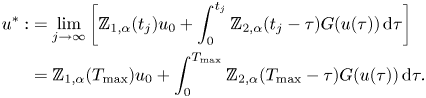 \begin{align*} {u}^{*}:&=\lim_{j\to\infty}\left[{\mathbb{Z}_{1,\alpha}(t_j){u}_{0}+\int_{0}^{t_j}\mathbb{Z}_{2,\alpha}(t_j-\tau)G(u(\tau))\,{\textrm{d}} \tau}\right]\\ &=\mathbb{Z}_{1,\alpha}(T_{\max}){u}_{0}+\int_{0}^{T_{\max}}\mathbb{Z}_{2,\alpha}(T_{\max}-\tau)G(u(\tau))\,{\textrm{d}} \tau. \end{align*}
This result helps us to enlarge the solution  ${u}$ of the problem (P1) over the interval
  $[0,T_{\max }]$. Therefore, lemma 3.2 is available to extend
  ${u}$ to an interval that is larger than
  $[0,T_{\max }]$. This fact contradicts our definition of
  $T_{\max }.$
3.2 Well-posedness results under the second assumption on the initial function
First of all, let us introduce the important nonlinear estimate for problem (P1). To achieve this aim, we need the following lemma about the Gamma function, that can be found in [Reference Furioli, Kawakami, Ruf and Terraneo22, lemma 3.3].
Lemma 3.4 For any  $p,q\ge 1$, there exists a positive constant
  $\bar {M}$ such that
 \[ \left[{\Gamma(pq+1)}\right]^{\frac{1}{q}}\le \bar{M}\Gamma(p+1)q^{p}. \]
Lemma 3.5 Let  $u,v\in {L^{\Xi }(\mathbb {R}^{N})}$ and
  $\mathcal {V}=\max \{\left \| {u} \right \|_{\Xi },\left \| {v} \right \|_{\Xi }\}.$ Then, for any
  $h\ge p$, the following estimate holds
 \[ \left\| {G(u)-G(v)} \right\|_{L^{h}}\le \mathscr{C}_h\mathcal{V}^{m-1}\sum_{j=0}^{\infty}(3h\kappa\mathcal{V}^{p})^{j}\left\| {u-v} \right\|_{\Xi}. \]
Proof. From (1.2), by using Taylor expansion, for any  $u,v\in {L^{\Xi }(\mathbb {R}^{N})},$ one has
 \begin{align} \left\| {G(u)-G(v)} \right\|_{L^{h}}&\le L\sum_{j=0}^{\infty}\frac{\kappa^{j}}{j!} \left\| {u-v} \right\|_{L^{3h}}\notag\\ &\quad \times\left({\left\| {u} \right\|_{L^{3hpj}}^{pj}\left\| {u} \right\|_{L^{3h(m-1)}}^{m-1}+\left\| {v} \right\|_{L^{3hpj}}^{pj}\left\| {v} \right\|_{L^{3h(m-1)}}^{m-1}}\right), \end{align}
where we have used the Hölder inequality with  $\frac {1}{h}=\frac {1}{3h}+\frac {1}{3h}+\frac {1}{3h}$. By the embedding stated in lemma 2.7, the estimate (3.9) becomes
 \begin{align} \left\| {G(u)-G(v)} \right\|_{L^{h}} &\le\frac{2L\mathcal{V}^{m-1}(\Gamma(3hp^{{-}1}+1))^{\frac{1}{3h}}}{\left({\Gamma(3h(m-1)p^{{-}1}+1)}\right)^{\frac{-1}{3h}}} \left\| {u-v} \right\|_{\Xi}\notag\\ &\quad \times \sum_{j=0}^{\infty}\left({\frac{\kappa^{j}}{j!}\mathcal{V}^{pj}\left[{\Gamma(3hj+1)}\right]^{\frac{1}{3h}}}\right). \end{align}
It follows from lemma 3.4 that
 \[ \left[{\Gamma(3hj+1)}\right]^{\frac{1}{3h}}\le \bar{M}\Gamma\left({j+1}\right)(3h)^{j}=\bar{M}(3h)^{j}j!. \]
Based on the above results, the following approximation is satisfied
 \begin{equation} \left\| {G(u)-G(v)} \right\|_{L^{h}}\le\frac{2L\mathcal{V}^{m-1}(\Gamma(3hp^{{-}1}+1))^{\frac{1}{3h}}}{\left({\Gamma(3h(m-1)p^{{-}1}+1)}\right)^{\frac{-1}{3h}}} \left\| {u-v} \right\|_{\Xi}\sum_{j=0}^{\infty}(3h\kappa\mathcal{V}^{p})^{j}. \end{equation}
3.2.1 Local-in-time solution
Theorem 3.6 Let  $u_0$ be in
  ${L^{\Xi }(\mathbb {R}^{N})}$ with sufficiently small data and
  $h>\max \{p,\frac {N}{4}\}$. Then there exists a locally unique mild solution to problem (4.3), belonging to an open ball centred at the origin with radius
  $\varepsilon <(3h\kappa )^{\frac {-1}{p}}$.
Proof. Our proof starts with the observation that
 \begin{equation} \left\| {\mathbb{Z}_{1,\alpha}(t)u_0} \right\|_{\Xi}\le\left\| {u_0} \right\|_{\Xi},\quad t>0, \end{equation}
where we have used lemma 2.9. In addition, for any  $u,v\in L^{\infty }\left ({0,T;{L^{\Xi }(\mathbb {R}^{N})}}\right ),\ T>0$, lemma 3.5 implies for a fixed constant
  $h>\max \{p,\frac {N}{4}\}$ and
  $t\in (0,T)$ that
 \begin{align*} &\int_{0}^{t}(t-\tau)^{\alpha\left({1-\frac{N}{4h}}\right)-1}\left\| {G(u(\tau))-G(v(\tau))} \right\|_{L^{h}}\,{\textrm{d}} \tau\\ &\quad\le \mathscr{C}_h\sum_{j=0}^{\infty}(3h\kappa)^{j}\int_{0}^{t}(t-\tau)^{\alpha\left({1-\frac{N}{4h}}\right)-1}\left\| {u(\tau)-v(\tau)} \right\|_{\Xi}[\mathcal{V}(\tau)]^{m-1+pj}\,{\textrm{d}} \tau\\ &\quad\le \frac{\mathscr{C}_hT^{\alpha\left({1-\frac{N}{4h}}\right)}}{\alpha\left({1-\frac{N}{4h}}\right)}\left\| {u-v} \right\|_{L^{\infty}_{T}\Xi}\left\| {\mathcal{V}} \right\|^{m-1}_{L^{\infty}_{T}\Xi}\sum_{j=0}^{\infty}(3h\kappa\left\| {\mathcal{V}} \right\|^{p}_{L^{\infty}_{T}\Xi})^{j}, \end{align*}
here we set  $\mathcal {V}(t)=\max \{\left \| {u(t)} \right \|_{\Xi },\left \| {v(t)} \right \|_{\Xi }\}$. Next, for purpose of using the fixed point principle, let us define the following mapping
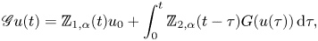 \begin{equation} \mathscr{G}u(t)=\mathbb{Z}_{1,\alpha}(t){u}_{0}+\int_{0}^{t}\mathbb{Z}_{2,\alpha}(t-\tau)G(u(\tau))\,{\textrm{d}} \tau, \end{equation}
which maps a closed ball  $B_{L^{\infty }\left ({0,T;{L^{\Xi }(\mathbb {R}^{N})}}\right )}(0,\varepsilon )$ to itself, provided that
  $\varepsilon <(3h\kappa )^{\frac {-1}{p}}$ and
  $T$ satisfies
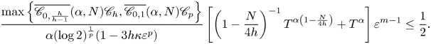 \[ \frac{\max\left\{\overline{\mathscr{C}_{0,\frac{h}{h-1}}}(\alpha,N)\mathscr{C}_h,\overline{\mathscr{C}_{0,1}}(\alpha,N)\mathscr{C}_p\right\}}{\alpha(\log 2)^{\frac{1}{p}}(1-3h\kappa\varepsilon^{p})}\left[{\left({1-\frac{N}{4h}}\right)^{{-}1}T^{\alpha\left({1-\frac{N}{4h}}\right)}+T^{\alpha}}\right]\varepsilon^{m-1}\le\frac{1}{2}. \]
We first prove the invariance of  $B_{L^{\infty }\left ({0,T;{L^{\Xi }(\mathbb {R}^{N})}}\right )}(0,\varepsilon )$ under the action of
  $\mathscr {G}$. Indeed, the Young convolution inequality and lemma 2.3 imply
 \begin{align} &\left\| {\int_{\mathbb{R}^{N}}\mathbb{K}_{2,\alpha} (t-\tau,x-y)\left[{G(u(\tau,y))-G(v(\tau,y))}\right]\,{\textrm{d}}y} \right\|_{L^{\infty}}\nonumber\\ &\quad\le\left\| {\mathbb{K}_{2,\alpha} (t-\tau,x)} \right\|_{L^{\frac{h}{h-1}}}\left\| {G(u(\tau))-G(v(\tau))} \right\|_{L^{h}}\nonumber\\ &\quad\le\overline{\mathscr{C}_{0,\frac{h}{h-1}}}(\alpha,N)(t-\tau)^{\alpha\left({1-\frac{N}{4h}}\right)-1}\left\| {G(u(\tau))-G(v(\tau))} \right\|_{L^{h}}. \end{align}
This result leads us to
 \[ \left\| {\mathscr{G}u-\mathscr{G}v} \right\|_{L^{\infty}_{T}{L^{\infty}_{x}}}\le \overline{\mathscr{C}_{0,\frac{h}{h-1}}}(\alpha,N)\int_{0}^{t}(t-\tau)^{\alpha\left({1-\frac{N}{4h}}\right)-1}\left\| {G(u(\tau))-G(v(\tau))} \right\|_{L^{h}}\,{\textrm{d}} \tau. \]
In (3.14) and the above inequality, if we take  $v\equiv 0$, then from the property of geometric series, the following holds
 \begin{align*} &\left\| {\mathscr{G}u-\mathbb{Z}_{1,\alpha}({\cdot})u_{0}} \right\|_{L^{\infty}_{T}{L^{\infty}_{x}}}\\ &\quad \le\overline{\mathscr{C}_{0,\frac{h}{h-1}}}(\alpha,N)\mathscr{C}_h\left[\alpha\left({1-\frac{N}{4h}}\right)\right]^{{-}1}T^{\alpha\left({1-\frac{N}{4h}}\right)}\varepsilon^{m}\left[{\sum_{j=0}^{\infty}(3h\kappa\varepsilon^{p})^{j}}\right]\\ &\quad =\overline{\mathscr{C}_{0,\frac{h}{h-1}}}(\alpha,N)\mathscr{C}_h\left[\alpha\left({1-\frac{N}{4h}}\right)\right]^{{-}1}T^{\alpha\left({1-\frac{N}{4h}}\right)}\varepsilon^{m}(1-3h\kappa\varepsilon^{p})^{{-}1}. \end{align*}
Similarly, we also obtain the following estimate for the  ${L^{p}(\mathbb {R}^{N})}$ norm
 \begin{align*} \left\| {\mathscr{G}u-\mathbb{Z}_{1,\alpha}u_{0}} \right\|_{L^{\infty}_{T}{L^{p}_{x}}}&\le \overline{\mathscr{C}_{0,1}}(\alpha,N)\mathscr{C}_p\alpha^{{-}1}T^{\alpha}\varepsilon^{m} \left[{\sum_{j=0}^{\infty}(3h\kappa\varepsilon^{p})^{j}}\right]\\ &=\overline{\mathscr{C}_{0,1}}(\alpha,N)\mathscr{C}_p\alpha^{{-}1}T^{\alpha}\varepsilon^{m}(1-3p\kappa\varepsilon^{p})^{{-}1}. \end{align*}
It follows from the above results that
 \begin{align*} \left\| {\mathscr{G}u} \right\|_{L^{\infty}_{T}\Xi}&\le \left\| {\mathbb{Z}_{1,\alpha}u_{0}} \right\|_{L^{\infty}_{T}\Xi}+(\log 2)^{\frac{-1}{p}}\\ &\quad \times \left({\left\| {\mathscr{G}u-\mathbb{Z}_{1,\alpha}u_{0}} \right\|_{L^{\infty}_{T}{L^{\infty}_{x}}}+\left\| {\mathscr{G}u-\mathbb{Z}_{1,\alpha}u_{0}} \right\|_{L^{\infty}_{T}{L^{p}_{x}}}}\right)\\ &\le \left\| {{u}_{0}} \right\|_{\Xi}+\frac{\max\left\{\overline{\mathscr{C}_{0,\frac{h}{h-1}}}(\alpha,N)\mathscr{C}_h,\overline{\mathscr{C}_{0,1}}(\alpha,N)\mathscr{C}_p\right\}}{\alpha(\log 2)^{\frac{1}{p}}(1-3h\kappa\varepsilon^{p})}\\ &\quad \times \left[{\left({1-\frac{N}{4h}}\right)^{{-}1}T^{\alpha\left({1-\frac{N}{4h}}\right)}+T^{\alpha}}\right]\varepsilon^{m}\le\varepsilon, \end{align*}
where we have used the smallness assumption for the initial data function that  $2\left \| {u_0} \right \|_{\Xi }\le \varepsilon <(3h\kappa )^{\frac {-1}{p}}.$ Hence, the invariance property of
  $\mathscr {G}$ is ensured. Furthermore, by using analogous arguments and the chosen time
  $T$, we can easily show that
  $\mathscr {G}$ is a strict contraction on
  $B_{L^{\infty }\left ({0,T;{L^{\Xi }(\mathbb {R}^{N})}}\right )}(0,\varepsilon )$. Then, the Banach principle argument yields that our problem has a unique local-in-time mild solution in
  $L^{\infty }\left ({0,T;{L^{\Xi }(\mathbb {R}^{N})}}\right )$ and the proof is complete.
3.2.2 Global-in-time well-posedness results
Lemma 3.7 (see [Reference Chen, Gao, Garrido-Atienza and Schmalfuß14, lemma 8)]
Let  $m,n>-1$ such that
  $m+n>-1$. Then
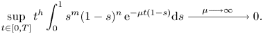 \[ \sup _{t \in[0, T]} t^{h} \int_{0}^{1} s^{m}(1-s)^{n} \,{\textrm{e}}^{-\mu t(1-s)} \mathrm{d} s\xrightarrow{{\quad\mu\longrightarrow\infty\quad}}0. \]
Definition 3.8 Let  $X$ be a Banach space. Then, we denote by
  $L^{\infty }_{a,b}\left ({(0,T];X}\right )$ the subspace of
  $L^{\infty }(0,T;X)$ such that
 \[ \sup_{t \in(0, T]}t^{a}\,{\textrm{e}}^{{-}bt}\left\| {\varphi(t)} \right\|_X<\infty,\quad \varphi\in L^{\infty}_{a,b}\left({(0,T];X}\right). \]
for some positive numbers  $a,b.$
Theorem 3.9 Assume that the initial function  ${u}_{0}$ belongs to
  ${L^{\Xi }_{0}(\mathbb {R}^{N})}$ and
  $m=1$. Then, problem (P1) has a unique solution in
  $C\left ({(0,T];{L^{q}(\mathbb {R}^{N})}}\right )\cap L^{\infty }_{a,b}\left ({(0,T];{L^{\Xi }_{0}(\mathbb {R}^{N})}}\right )$ for
  $a\in (0,1)$ and some
  $b_0>0$. Furthermore, if
  $N<4p,a<\min \{\frac {1}{2},\frac {\alpha N}{4p}\}$, we have
 \begin{equation} \left\| {u(t)} \right\|_{L^{p}}\le Ct^{{-}a}\,{\textrm{e}}^{b_0t}\left\| {u_0} \right\|_{\Xi}. \end{equation}
Proof. The proof starts by handling the nonlinear source term on the RHS of the first equation of problem (P1). For every  $u\in L^{\infty }_{a,b}\left ({(0,T];{L^{\Xi }_{0}(\mathbb {R}^{N})}}\right )$, we can choose two functions
  $u_1,u_2$ such that
 \begin{equation} \begin{cases} \displaystyle u(t)=u_1(t)+u_2(t)\quad & \forall t\in(0,T],\\ \displaystyle u_1(t)\in C_0^{\infty}(\mathbb{R}^{N}), & \forall t\in(0,T],\\ \displaystyle\left\| {u_2(t)} \right\|_{\Xi}<(3h\kappa {2^{p-1}})^{\frac{-1}{p}}, & \forall t\in(0,T]. \end{cases} \end{equation}
For brevity, we set
 \[ \mathscr{C}_T:=\sup_{u\in L^{\infty}_{a,b}\left({(0,T];{L^{\Xi}_{0}(\mathbb{R}^{N})}}\right)}\left\{\sup_{t \in(0, T]}\Big\{|u_1(t)|:u_1(t)\ \text{satisfies}\ (3.16) \Big\}\right\}. \]
 Then, for any  $h\in [p,\infty )$,
 \[ \left\| {G(u(t))-G(v(t))} \right\|_{L^{h}}\le L\left\| {|u(t)-v(t)|\left({{\textrm{e}}^{\kappa|u_1(t)+u_2(t)|^{p}}+{\textrm{e}}^{\kappa|v_1(t)+v_2(t)|^{p}}}\right)} \right\|_{L^{h}}. \]
 Using the inequality  $(a+b)^{q}<{2^{p-1}}(a^{q}+b^{q})$ for
  $a,b>0,q>1$, we obtain
 \begin{align*} &\left\| {G(u(t))-G(v(t))} \right\|_{L^{h}}\\ &\quad \le L\left\| {|u(t)-v(t)|\left({{\textrm{e}}^{\kappa {2^{p-1}}|u^{p}_1(t)+u^{p}_2(t)|}+{\textrm{e}}^{\kappa {2^{p-1}}|v^{p}_1(t)+v^{p}_2(t)|}}\right)} \right\|_{L^{h}}\\ &\quad \le L\,{\textrm{e}}^{\kappa {2^{p-1}}\mathscr{C}_T^{p}}\left\| {|u(t)-v(t)|\left({{\textrm{e}}^{\kappa {2^{p-1}}|u^{p}_2(t)|}+{\textrm{e}}^{\kappa {2^{p-1}}|v^{p}_2(t)|}}\right)} \right\|_{L^{h}}. \end{align*}
Then, it follows from lemmas 3.5 and 2.7 that
 \begin{align} &\left\| {G(u(t))-G(v(t))} \right\|_{L^{h}}\notag\\ &\quad \le C\left\| {u(t)-v(t)} \right\|_{\Xi}\sum_{j=0}^{\infty}\left(3h\kappa {2^{p-1}}\left[{\max_{w\in\{u_2,v_2\}}\left\{\sup_{t \in(0, T]}\left\| {w(t)} \right\|_{\Xi}\right\}}\right]^{p}\right)^{j}. \end{align}
Then, by (3.16), the following nonlinear estimate holds
 \begin{equation} \left\| {G(u(t))-G(v(t))} \right\|_{L^{h}}\le C\left\| {u(t)-v(t)} \right\|_{\Xi}. \end{equation}
Now, we define the following set
 \[ \mathbf{O}:=\left\{u\in C\left({(0,T];{L^{p}(\mathbb{R}^{N})}}\right)\cap L^{\infty}_{a,b}\left({(0,T];{L^{\Xi}_{0}(\mathbb{R}^{N})}}\right)\big|\sup_{t\in(0,T]}t^{a}\,{\textrm{e}}^{{-}bt}\left\| {u(t)} \right\|_{\Xi}<\infty\right\} \]
and a mapping  $\mathscr {H}$ that maps
  $\mathbf {O}$ to itself, formulated by
 \begin{equation} \mathscr{H}u(t)=\mathbb{Z}_{1,\alpha}(t){u}_{0}+\int_{0}^{t}\mathbb{Z}_{2,\alpha}(t-\tau)G(u(\tau))\,{\textrm{d}} \tau. \end{equation}
Since  $u_0\in {L^{\Xi }_{0}(\mathbb {R}^{N})}$, lemma 2.1 ensures the continuity on
  $(0,T]$ of the first term on the RHS of (3.19). Furthermore, combining (3.18) and the same argument as in theorem 3.1, we have
 \[ \mathscr{H}u-\mathbb{Z}_{1,\alpha}{u}_{0}\in C\left({(0,T];{L^{p}(\mathbb{R}^{N})}}\right). \]
In addition, for any  $u\in \mathbf {O}$,
  $\mathscr {H}u$ is completely bounded in time. Notice also that
  $u\in L^{\infty }_{a,b}\left ({(0,T];{L^{\Xi }_{0}(\mathbb {R}^{N})}}\right )$. Then, the Young convolution inequality and lemma 2.3 imply that
 \begin{align*} &\left\| {\mathscr{H}u(t)-\mathbb{Z}_{1,\alpha}(t)u_0} \right\|_{L^{\infty}}\\ &\quad \le\int_{0}^{t}\left\| {\mathbb{Z}_{2,\alpha}(t-\tau)G(u(\tau))} \right\|_{L^{\infty}}\,{\textrm{d}} \tau\\ &\quad \le\int_{0}^{t}(t-\tau)^{\alpha\left({1-\frac{ N}{4h}}\right)-1}\left\| {G(u(\tau))} \right\|_{L^{h}}\,{\textrm{d}} \tau,\quad \text{for}\ h>\max\left\{\frac{N}{4},p\right\}. \end{align*}
By using (3.18), we obtain
 \begin{align*} \left\| {\mathscr{H}u(t)-\mathbb{Z}_{1,\alpha}(t)u_0} \right\|_{L^{\infty}}&\le C\sup_{t \in(0, T]}\left\| {u(t)} \right\|_{\Xi}\left({\int_{0}^{t}(t-\tau)^{\alpha\left({1-\frac{ N}{4h}}\right)-1}\,{\textrm{d}} \tau}\right)\\ &=\frac{CT^{\alpha\left({1-\frac{ N}{4h}}\right)}}{\alpha\left({1-\frac{ N}{4h}}\right)}\sup_{t \in(0, T]}\left\| {u(t)} \right\|_{\Xi}. \end{align*}
Likewise, we also have
 \begin{align*} \left\| {\mathscr{H}u(t)-\mathbb{Z}_{1,\alpha}(t)u_0} \right\|_{L^{p}}&\le C\sup_{t \in(0, T]}\left\| {u(t)} \right\|_{\Xi}\left({\int_{0}^{t}(t-\tau)^{\alpha-1}\,{\textrm{d}} \tau}\right)\\ &=CT^{\alpha}{\alpha}^{{-}1}\sup_{t \in(0, T]}\left\| {u(t)} \right\|_{\Xi}. \end{align*}
 From two results above, lemmas 2.8 and 2.9, the conclusion  $\mathscr {H}u\in L^{\infty ,*}\left ({(0,T];{L^{\Xi }_{0}(\mathbb {R}^{N})}}\right )$ can be drawn through the following one
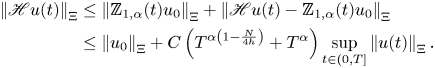 \begin{align*} \left\| {\mathscr{H}u(t)} \right\|_{\Xi}&\le\left\| {\mathbb{Z}_{1,\alpha}(t)u_0} \right\|_{\Xi}+\left\| {\mathscr{H}u(t)-\mathbb{Z}_{1,\alpha}(t)u_0} \right\|_{\Xi}\\ &\le\left\| {u_0} \right\|_{\Xi}+C\left({T^{\alpha\left({1-\frac{ N}{4h}}\right)}+T^{\alpha}}\right)\sup_{t \in(0, T]}\left\| {u(t)} \right\|_{\Xi}. \end{align*}
 We note that  $\mathbf {O}$ is a complete metric space with the metric
 \[ d_{\mathbf{O}}(u,v):=\sup_{t\in(0,T]}t^{a}\,{\textrm{e}}^{{-}bt}\left\| {u(t)-v(t)} \right\|_{\Xi}. \]
The remaining part of this proof is to show that  $\mathscr {H}$ is a strict contraction on
  $\mathbf {O}$ with respect to the above metric. Indeed, for any
  $u,v\in \mathbf {O}$, we have
 \begin{align} &t^{a}\,{\textrm{e}}^{{-}bt}\left\| {\mathscr{H}u(t)-\mathscr{H}v(t)} \right\|_{L^{p}+L^{\infty}}\nonumber\\ &\quad\le\int_{0}^{t}(t-\tau)^{\alpha-1}\left\| {\mathbb{Z}_{2,\alpha}(t-\tau)\left[{G(u(\tau))-G(v(\tau))}\right]} \right\|_{L^{p}+L^{\infty}}\,{\textrm{d}} \tau\nonumber\\ &\quad\le t^{a}\,{\textrm{e}}^{{-}bt}\int_{0}^{t}(t-\tau)^{\alpha-1}\left\| {G(u(\tau))-G(v(\tau))} \right\|_{L^{p}+L^{\infty}}\,{\textrm{d}} \tau\nonumber\\ &\quad\le Cd_{\mathbf{O}}(u,v)t^{a}\int_{0}^{t}\tau^{{-}a}\left[{(t-\tau)^{\alpha-1}+(t-\tau)^{\alpha\left({1-\frac{ N}{4h}}\right)-1}}\right]\,{\textrm{e}}^{{-}b(t-\tau)}\,{\textrm{d}} \tau. \end{align}
Using the substitution technique, the latter inequality becomes
 \begin{align*} &t^{a}\,{\textrm{e}}^{{-}bt}\left\| {\mathscr{H}u(t)-\mathscr{H}v(t)} \right\|_{L^{p}+L^{\infty}}\\ &\quad \le Cd_{\mathbf{O}}(u,v) t^{\alpha}\int_{0}^{1}\tau^{{-}a}(1-\tau)^{\alpha-1}\,{\textrm{e}}^{{-}bt(1-\tau)}\,{\textrm{d}} \tau\\ &\qquad+ Cd_{\mathbf{O}}(u,v) t^{\alpha\left({1-\frac{ N}{4h}}\right)}\int_{0}^{1}\tau^{{-}a}(1-\tau)^{\alpha\left({1-\frac{ N}{4h}}\right)-1}\,{\textrm{e}}^{{-}bt(1-\tau)}\,{\textrm{d}} \tau. \end{align*}
Choosing  $0< a<\alpha <1$ and
  $4h>N$, we use lemma 3.7 to obtain
 \[ \begin{cases} \displaystyle\lim_{b\to \infty}\sup_{t\in(0,T]}t^{\alpha}\int_{0}^{1}\tau^{{-}a}(1-\tau)^{\alpha-1}\,{\textrm{e}}^{{-}bt(1-r)}\,{\textrm{d}} \tau=0,\\ \displaystyle\lim_{b\to \infty}\sup_{t\in(0,T]}t^{\alpha\left({1-\frac{ N}{4h}}\right)}\int_{0}^{1}\tau^{{-}a}(1-\tau)^{\alpha\left({1-\frac{ N}{4h}}\right)-1}\,{\textrm{e}}^{{-}bt(1-r)}\,{\textrm{d}} \tau=0. \end{cases} \]
Hence, there exists a large number  $b_0$ such that the following holds
 \[ t^{a}\,{\textrm{e}}^{{-}b_0t}\left\| {\mathscr{H}u(t)-\mathscr{H}v(t)} \right\|_{L^{p}+L^{\infty}}\le\mathcal{L}(\log 2)^{{-}p}\,{\textrm{d}} _{\mathbf{O}}(u,v), \]
where  $\mathcal {L}$ is a positive constant less than 1. This implies that
 \[ d_{\mathbf{O}}(\mathscr{H}u,\mathscr{H}v)\le\mathcal{L}\,{\textrm{d}} _{\mathbf{O}}(u,v). \]
Therefore,  $\mathscr {H}$ has a unique fixed point in
  $\mathbf {O}$. Therefore, we can conclude that there exists a unique solution to problem (P1).
Next, let us verify the correctness of the statement (3.15) as  $N<4p$. Firstly, if
  $t\le 1$, we have
 \[ t^{a}\,{\textrm{e}}^{{-}b_0t}\left\| {\mathbb{Z}_{1,\alpha}(t)u_0} \right\|_{L^{p}}\le C\left\| {\mathbb{Z}_{1,\alpha}(t)u_0} \right\|_{L^{p}}\le C\left\| {u_0} \right\|_{L^{p}}\le C\left\| {u_0} \right\|_{\Xi}. \]
In addition, if  $t>1$, by using the Cauchy inequality and lemma 2.9, we obtain
 \begin{align*} t^{a}\,{\textrm{e}}^{{-}b_0t}\left\| {\mathbb{Z}_{1,\alpha}(t)u_0} \right\|_{L^{p}}&\le C\left\| {\mathbb{Z}_{1,\alpha}(t)u_0} \right\|_{\Xi}\\ &\le Ct^{a-\frac{\alpha N}{4p}}\left[\log\left({2t^{\frac{-\alpha N}{8}}}\right)\right]^{\frac{-1}{p}}\left\| {u_0} \right\|_{L^{p}}\le C\left\| {u_0} \right\|_{\Xi}, \end{align*}
where we have used the assumption that  $a\le \frac {\alpha N}{4p}.$ On the other hand, if
  $u\in L^{\infty }\left ({(0,T];{L^{\Xi }_{0}(\mathbb {R}^{N})}}\right ),$ we can use (3.18) to derive the following estimate
 \[ \left\| {G(u(t))} \right\|_{L^{p}}\le C\left\| {u(t)} \right\|_{\Xi}. \]
It follows immediately that
 \begin{align*} &t^{a}\,{\textrm{e}}^{{-}b_0t}\int_{0}^{t}(t-\tau)^{\alpha-1}\left\| {\mathbb{Z}_{2,\alpha}(t)(t-\tau)G(u(\tau))} \right\|_{L^{p}}\,{\textrm{d}} \tau\\ &\quad \le Ct^{a}\,{\textrm{e}}^{{-}b_0t}\int_{0}^{t}(t-\tau)^{\alpha-1}\left\| {\mathbb{Z}_{2,\alpha}(t-\tau)u(\tau)} \right\|_{\Xi}\,{\textrm{d}} \tau. \end{align*}
Thanks to the assumption that  $N<4p$, lemma 2.9 implies
 \begin{align*} t^{a}\,{\textrm{e}}^{{-}b_0t}\left\| {u(t)-\mathbb{Z}_{1,\alpha}(t)u_0} \right\|_{L^{p}}&\le Ct^{a}\,{\textrm{e}}^{{-}b_0t}\int_{0}^{t}(t-\tau)^{\alpha\left({1-\frac{N}{4p}}\right)-1}\\ &\quad \times \left[\log\left({1+(t-\tau)^{\frac{-\alpha N}{4}}}\right)\right]^{\frac{-1}{p}}\left\| {u(\tau)} \right\|_{L^{p}}\,{\textrm{d}} \tau. \end{align*}
Thanks to the Hölder inequality,
 \begin{align*} &t^{a}\,{\textrm{e}}^{{-}b_0t}\left\| {u(t)-\mathbb{Z}_{1,\alpha}(t)u_0} \right\|_{L^{p}}\\ &\quad \le C\left({t^{2a}\int_{0}^{t}(t-\tau)^{\alpha\left({1-\frac{N}{4p}}\right)-1}\left[\log\left({1+(t-\tau)^{\frac{-\alpha N}{4}}}\right)\right]^{\frac{-2}{p}}\tau^{{-}2a}\,{\textrm{e}}^{{-}2b_0(t-\tau)}\,{\textrm{d}} \tau}\right)^{\frac{1}{2}}\\ &\qquad \times\left({\int_{0}^{t}(t-\tau)^{\alpha\left({1-\frac{N}{4p}}\right)-1}\left[{\tau^{a}\,{\textrm{e}}^{{-}b_0{\tau}}\left\| {u({\tau})} \right\|_{L^{p}}}\right]^{2}\,{\textrm{d}}\tau}\right)^{\frac{1}{2}} \end{align*}
 To deal with the  $\log$ term, let us denote by
  $\gamma$ the infimum of the set
  $\{z>0: z>2 \log (1+z)\}$. If
  $t^{\frac {-\alpha N}{4}}>\gamma ,$ the results will be covered by the opposite case, for this reason, we only need to consider the case
  $t^{\frac {-\alpha N}{4}}>\gamma$. As
  $t^{\frac {-\alpha N}{4}}>\gamma$, thanks to lemma 3.7, the two following claims will be obtained.
Claim 1 If  $\tau \le t-\gamma ^{\frac {-4}{\alpha N}}$, we have
  $(t-\tau )^{\frac {\alpha N}{4}}<\gamma$. This one implies that
 \[ \log \left(1+(t-\tau)^{\frac{-\alpha N}{4}}\right)>\frac{(t-\tau)^{\frac{-\alpha N}{4}}}{2},\quad\text{for } 0<\tau\le t-\gamma^{\frac{-4}{\alpha N}}. \]
Based on the above inequality, one can derive that
 \begin{align} &t^{2a}\int_{0}^{t-\gamma^{\frac{-4}{\alpha N}}}(t-\tau)^{\alpha\left(1-\frac{N}{4 p}\right)-1}\left[\log \left(1+(t-\tau)^{\frac{-\alpha N}{4}}\right)\right]^{\frac{-2}{p}}\tau^{{-}2a}\,{\textrm{e}}^{{-}2b_0(t-\tau)}\,{\textrm{d}} \tau\nonumber\\ &\quad\le C t^{2a}\int_{0}^{t-\gamma^{\frac{-4}{\alpha N}}}(t-\tau)^{\alpha\left(1+\frac{N}{4 p}\right)-1}\tau^{{-}2a}\,{\textrm{e}}^{{-}2b_0(t-\tau)}\,{\textrm{d}} \tau\nonumber\\ &\quad\le Ct^{{}^{\alpha\left(1+\frac{N}{4 p}\right)}}\int_{0}^{1}(1-r)^{\alpha\left(1+\frac{N}{4 p}\right)-1}\tau^{{-}2a}\,{\textrm{e}}^{{-}2b_0t(1-\tau)}\,{\textrm{d}} \tau\le C. \end{align}
Claim 2 On the contrary, if  $t-r<\gamma ^{\frac {-4}{\alpha N}}$, we have
 \begin{align*} &t^{2a}\int_{t-\gamma^{\frac{-4}{\alpha N}}}^{t}(t-\tau)^{\alpha\left(1-\frac{N}{4 p}\right)-1}\left[\log\left(1+(t-\tau)^{\frac{-\alpha N}{4}}\right)\right]^{\frac{-2}{p}}\tau^{{-}2a}\,{\textrm{e}}^{{-}2b_0(t-\tau)}\,{\textrm{d}}r\\ &\quad\le Ct^{2a}[\log (1+\gamma)]^{\frac{-2}{p}} \int_{t-\gamma^{\frac{-4}{\alpha N}}}^{t}(t-\tau)^{\alpha\left(1-\frac{N}{4 p}\right)-1}\tau^{{-}2a}\,{\textrm{e}}^{{-}2b_0(t-\tau)}\,{\textrm{d}} \tau\\ &\quad\le t^{{}^{\alpha\left(1-\frac{N}{4 p}\right)}}\int_{0}^{1}(1-r)^{\alpha\left(1-\frac{N}{4 p}\right)-1}\tau^{{-}2a}\,{\textrm{e}}^{{-}2b_0t(1-\tau)}\,{\textrm{d}} \tau\le C. \end{align*}
Combining the above results, the triangle inequality and the inequality  $(a+b)^{2}\le 2(a^{2}+b^{2})$ we deduce
 \[ t^{2a}\,{\textrm{e}}^{{-}2b_0t}\left\| {u(t)} \right\|_{L^{p}}^{2}\le C\left\| {u_0} \right\|^{2}_{\Xi}+C\int_{0}^{t}(t-\tau)^{\alpha\left({1-\frac{N}{4p}}\right)-1}\left[{\tau^{a}\,{\textrm{e}}^{{-}b_0\tau}\left\| {u(\tau)} \right\|_{L^{p}}}\right]^{2}\,{\textrm{d}}\tau. \]
Now, we are in the position to apply the Grönwall inequality to achieve the desired result
 \[ \left\| {u(t)} \right\|_{L^{p}}\le Ct^{{-}a}\,{\textrm{e}}^{b_0t}\left\| {u_0} \right\|_{\Xi}. \]
4. Time-fractional Cahn–Hilliard on the unbounded domain $\mathbb {R}^{N}$

In this section, we consider the following time-fractional Cahn–Hilliard on  $\mathbb {R}^{N}$
 \begin{equation} \begin{cases} \displaystyle \partial^{\alpha}_{0|t} u(t,x) + \Delta^{2} u(t,x) - \Delta F(t,x,u)=0, & \mbox{in}\quad\mathbb{R}^{+}\times\mathbb{R}^{N}, \\ \displaystyle u(0,x)= u_0(x), & \mbox{in} \quad \mathbb{R}^{N}. \end{cases} \end{equation}
Lemma 4.1 (see [Reference Robinson, Rodrigo and Sadowski35])
If  $1\le b \le p \le d$ and
  $v \in L^{b}(\mathbb {R}^{N}) \cap L^{d}(\mathbb {R}^{N})$, then
  $v \in L^{p}(\mathbb {R}^{N})$ where
 \begin{equation} \|u\|_{L^{p}} \le \|u\|_{L^{b}}^{\alpha} \|u\|_{L^{d}}^{1-\alpha},\quad \frac{1}{p}= \frac{\alpha}{b}+\frac{1-\alpha}{{\textrm{d}}} \end{equation}
We first consider the following linear problem
 \begin{equation} \begin{cases} D^{\alpha}_t \widehat u (t,\xi) + |\xi|^{4} \widehat u (t,\xi) = \widehat {\Delta F } (t,\xi) , & \mbox{in} \quad (0,T] \times \mathbb{R}^{N} , \\ \widehat u(0,\xi)= \widehat u_0(\xi), & \mbox{in} \quad \mathbb{R}^{N}, \end{cases} \end{equation}
As in the previous section, by the Duhamel principle, the solution to problem (4.2) is given by
 \begin{equation} \widehat u (t,\xi)= E_{\alpha,1} ({-}t^{\alpha} |\xi|^{4}) \widehat u_0(\xi)+ \int_0^{t} (t-s)^{\alpha-1} E_{\alpha,\alpha} (- (t-\tau)^{\alpha} |\xi|^{4}) \widehat {\Delta F } (\tau,\xi)\,{\textrm{d}}\xi \end{equation}
 To deal with the source term in the form of  $\Delta H$, we have to do some revisions to the generalized formula of solution. Applying the fact that
  $\frac {{\textrm {d}}}{{\textrm {d}}x} (f(x)*g(x) )= ( \frac {{\textrm {d}}}{{\textrm {d}}x}f(x) )* g(x),$ we immediately have that
 \begin{align*} \Delta \mathbb{Z}_{i,\alpha}(t) v(x)&= \Delta \Big( \mathbb{K}_{i,\alpha} (t,x) * v(t,x)\Big)=\Big( \Delta v(t,x) \Big)* \mathbb{K}_{i,\alpha} (t,x)\\ & = \int_{\mathbb{R}^{N}} \Delta \mathbb{K}_{i,\alpha} (t,x-y) v(t,y)\,{\textrm{d}}y,\quad i=1,2. \end{align*}
Next, we show that  $u$ satisfies the following equality
 \[ u(t,x)= \underbrace{\mathbb{Z}_{1,\alpha} (t) u_0(x)}_{\mathscr I_1(t,x)}+ \underbrace{\int_0^{t} \Delta \mathbb{Z}_{2,\alpha} (t-s) F(u(s,x))\,{\textrm{d}}s}_{\mathscr I_2(t,x)}. \]
Using (2.2), we infer that the Fourier transform of the first quantity  $\mathscr I_1(t,x)$ is given by
 \[ \widehat {\mathscr I_1} (t,\xi)= \widehat {\mathbb{K}_{1,\alpha} * u_0}=\widehat {\mathbb{K}_{1,\alpha} } \widehat { u_0} = E_{\alpha,1} ({-}t |\xi|^{4}) \widehat u_0(\xi). \]
It is not difficult to verify that the Fourier transformation of the given second quantity  $\mathscr I_2 (t, x)$ is as follows:
 \begin{align*} \widehat {\mathscr I_2} (t,\xi)&= \int_{\mathbb{R}^{N} } \,{\textrm{e}}^{{-}i <\xi, x>} \int_0^{t} \Delta \mathbb{Z}_{2,\alpha} (t-\tau) F(u(\tau,x))\,{\textrm{d}} \tau \,{\textrm{d}}x\\ &= \int_0^{t} \Big( \int_{\mathbb{R}^{N} } \,{\textrm{e}}^{{-}i <\xi, x>} \mathbb{K}_{2,\alpha} (t-\tau) \Delta F(u(\tau,x)) \,{\textrm{d}}x \Big) \,{\textrm{d}}\tau \\ &= \int_0^{t} \mathcal{F} \Big( \Big( \Delta F(u(\tau,x)) \Big)* \mathbb{K}_{2,\alpha} (t-\tau,x)\Big) \,{\textrm{d}}\tau\\ &= \int_0^{t} \widehat{\mathbb{K}_{2,\alpha}} (t-\tau,\xi) \widehat {\Delta F} (u(\tau,x)) \,{\textrm{d}}\tau \end{align*}
where we have used the formula  $\mathcal {F} (f*g)= \widehat f \widehat g,$ and from the following fact
 \[ \widehat{\mathbb{K}_{2,\alpha}} (t-\tau,\xi) = (t-\tau)^{\alpha-1} E_{\alpha,\alpha} \big(-(t-\tau)^{\alpha} |\xi|^{4}\big) , \]
we arrive at the following equality
 \[ \widehat {\mathscr I_2} (t,\xi)= \int_0^{t} (t-s)^{\alpha-1} E_{\alpha,\alpha} (- (t-s)^{\alpha} |\xi|^{4}) \widehat {\Delta F} (u (s,\xi) )\,{\textrm{d}}\xi. \]
We establish the local well-posedness of solutions for problem (P2) with small initial data in  $\mathbb {R}^{N}$ by using Kato's method (see [Reference Liu, Wang and Zhao29]). More precisely, our main result in this section can be stated as follows.
Theorem 4.2 Let  $\alpha >\frac {1}{2}$ and
  $\mathcal {E}>0$ be a sufficientl y small constant. Assume that
 \[ \left\| {u_0} \right\|_{L^{\infty}}\le\mathcal{E}\quad\text{and}\quad \max_{|z| \le \mathcal{E} } \sum_{k=1}^{L} \Big| D^{k} F(z)\Big| =\mathcal{A}. \]
Then, problem (P2) has a unique solution  $u(t,x)$ on the strip
 \[ \mathscr P_{ T_0}= \Big\{ (t,x): 0< t \le T_0,\ x \in \mathbb{R}^{N} \Big \} \]
such that
 \begin{equation} \|u(t)\|_{L^{\infty}} \le 2 \mathcal{E},\quad 0\le t \le T_0. \end{equation}
Here  $T_0$ is given by
 \begin{align} T_0 &\le \min \Bigg\{ 1, \bigg( \frac{\alpha \Gamma(\alpha/2+1)} {4\Big( \int_{\mathbb{R}^{N}} \Big| \overline{\mathscr B}_2 (z) \Big|{\textrm{d}}z\Big) \mathcal{A} \Gamma \left( \frac{3}{2} \right) \Gamma(\alpha/2) } \bigg)^{\frac{2}{\alpha}},\notag\\ &\quad \times \bigg( \frac{\alpha \Gamma(\alpha/2+1)} {4\Big( \int_{\mathbb{R}^{N}} \Big| \overline{\mathscr B}_2 (z) \Big|{\textrm{d}}z\Big) \mathcal{A} \Gamma \left( \frac{3}{2} \right) } \bigg)^{\frac{2}{\alpha}} \Bigg\}. \end{align}
In addition, for each partition  $0< t_1 < t_2<\cdots < t_N < t \le T_0$, it holds the following estimate
 \[ \|D^{k} u(t)\|_{L^{\infty}}\le (t-t_k)^{-\frac{\alpha k}{4}} \mathcal{Q}_k (\mathcal{E}, \alpha, t_k-t_1, t-t_k), \quad t_k < t \le T_0, \]
where  $\mathcal {Q}_k$ is a continuous increasing function of
  $t-t_k$.
Proof. Let us consider the following integral
 \begin{equation} u(t,x)=\int_{\mathbb{R}^{N}} \mathbb{K}_{1,\alpha} (t,x-y) u_0(y)\,{\textrm{d}}y + \int_0^{t} \int_{\mathbb{R}^{N}} \mathbb{K}_{2,\alpha} (t-\tau,x-y) F(u(\tau,y))\,{\textrm{d}} \tau. \end{equation}
First, we show that for  $T_0$ defined by (4.5), the integro-differential equation (4.6) admits a unique continuous solution
  $u(t, x)$ on the strip
  $\mathscr P_{ T_0}$. We apply the successive approximations method given in [Reference Liu, Wang and Zhao29]. Let us consider the following sequence
 \begin{align} v_0(t,x)&= u_0(x),\notag\\ v_n(t,x)&= \int_{\mathbb{R}^{N}}\mathbb{K}_{1,\alpha} (t,x-y) u_0(y)\,{\textrm{d}}y\notag\\ &\quad + \int_0^{t} \int_{\mathbb{R}^{N}} \Delta \mathbb{K}_{2,\alpha} (t-\tau,x-y) F(v_{n-1}(\tau,y))\,{\textrm{d}}y \,{\textrm{d}}\tau \end{align}
 \begin{align} &= \mathbb{Z}_{1,\alpha} (t) u_0(x)+ \int_0^{t} \Delta \mathbb{Z}_{2,\alpha} (t-\tau) F(v_{n-1}(\tau,x))\,{\textrm{d}} \tau. \end{align}
It is easy to see that  $v_n$ is well defined on
  $[0, \infty ) \times \mathbb {R}^{N}$. For
  $n=0$, we have immediately that
  $\|v_0\|_{L^{\infty }} = \|u_0\|_{L^{\infty }} \le \mathcal {E}$. Thus, we apply inequality (2.9) for
  $p=1$ to derive
 \begin{equation} \Big\|\mathbb{K}_{1,\alpha} (t)\Big\|_{L^{1}(\mathbb{R}^{N})} \le \frac{ \Big( \int_{\mathbb{R}^{N}} \Big| \overline{\mathscr B}_0 (z) \Big|{\textrm{d}}z\Big) \Gamma (1) }{ \Gamma (1) } {\le} 1, \end{equation}
where we have used the fact that  $\int _{\mathbb {R}^{N}} \Big | \overline {\mathscr B}_0 (z) \Big |{\textrm {d}}z= \int _{\mathbb {R}^{N}} \Big | \int _{\mathbb {R}^{N}} \,{\textrm {e}}^{i z\vartheta } \,{\textrm {e}}^{-|\vartheta |^{4}} {\textrm {d}}\vartheta \Big |{\textrm {d}}z=1$. Now, we apply induction method to show the following inequality
 \begin{equation} \left|\mkern-1.5mu\left|\mkern-1.5mu\left| {v_j} \right|\mkern-1.5mu\right|\mkern-1.5mu\right|_{\mathscr P_{ T_0}}= \sup_{(t,x) \in {\mathscr P_{ T_0}}} |v_j(t,x)| \le 2 \mathcal{E},\quad j \ge 1. \end{equation}
For  $n=1$, we recall the result based on the Young convolution inequality and (4.9) as follows
 \begin{align} \Bigg\|\int_{\mathbb{R}^{N}} \mathbb{K}_{1,\alpha} (t,\cdot{-}y) u_0(y)\,{\textrm{d}}y\Bigg\|_{L^{\infty}}&=\Big\| \mathbb{K}_{1,\alpha} (t) * u_0 \Big\|_{L^{\infty}}\notag\\ &\le \| \mathbb{K}_{1,\alpha} (t) \|_{L^{1}(\mathbb{R}^{N})} \| u_0 \|_{L^{\infty}} \le \| u_0 \|_{L^{\infty}} \le \mathcal{E}. \end{align}
Let us continue to verify that
 \begin{align*} &\Bigg\|\int_0^{t} \Delta \mathbb{Z}_{2,\alpha} (t-\tau) F(v_{0}(\tau,x))\,{\textrm{d}} \tau \Bigg\|_{L^{\infty}}\\ &\quad =\Bigg\|\int_0^{t} \int_{\mathbb{R}^{N}} \Delta \mathbb{K}_{2,\alpha} (t-\tau,x-y) F(v_{0}(\tau,y)) {\textrm{d}}y \,{\textrm{d}}\tau \Bigg\|_{L^{\infty}} \\ &\quad \le \int_0^{t} \Bigg\| \int_{\mathbb{R}^{N}} \Delta \mathbb{K}_{2,\alpha} (t-\tau,x-y) F(v_{0}(\tau,y)) {\textrm{d}}y \Bigg\|_{L^{\infty}} \,{\textrm{d}}\tau\\ &\quad \le \int_0^{t} \| \Delta \mathbb{K}_{2,\alpha} (t-\tau,x) \|_{L^{1}(\mathbb{R}^{N})} \| F(v_{0}(\tau,x)) \|_{L^{\infty}} \,{\textrm{d}}\tau. \end{align*}
By taking  $p = 1$ and
  $k=2$ into inequality (2.7), we obtain the following bound immediately
 \begin{align} \Big\|\Delta \mathbb{K}_{2,\alpha} (t,x) \Big\|_{L^{1}(\mathbb{R}^{N})}&= \Big\| D^{2} \mathbb{K}_{2,\alpha} (t,x) \Big\|_{L^{1}(\mathbb{R}^{N})}\le \frac{ \Big( \int_{\mathbb{R}^{N}} \Big| \overline{\mathscr B}_2 (z) \Big|{\textrm{d}}z\Big) \Gamma \left( \frac{3}{2} \right)}{\Gamma \left( 1+\frac{\alpha}{2} \right)} t^{\frac{\alpha}{2}-1} , \end{align}
which combined with the condition
 \begin{equation} \| F(v_{0}(s,x)) \|_{L^{\infty}} \le \mathcal{A} \sup_{(t,x) \in \mathscr S_0} |v_0(t,x)|, \end{equation}
imply
 \begin{align} &\Bigg\|\int_0^{t} \Delta \mathbb{Z}_{2,\alpha} (t-s) F(v_{0}(s,x))\,{\textrm{d}}s\Bigg\|_{L^{\infty}}\notag\\ &\quad \le \frac{ \Big( \int_{\mathbb{R}^{N}} \Big| \overline{\mathscr B}_2 (z) \Big|{\textrm{d}}z\Big) \mathcal{A} \Gamma \left( \frac{3}{2} \right)}{\Gamma \left( 1+\frac{\alpha}{2} \right)} \sup_{(t,x) \in \mathscr S_0} |v_0(t,x)| \int_0^{t} (t-s)^{\alpha/2-1} \,{\textrm{d}}s \nonumber\\ & \quad \le \frac{ \Big( \int_{\mathbb{R}^{N}} \Big| \overline{\mathscr B}_2 (z) \Big|{\textrm{d}}z\Big) \mathcal{A} \Gamma \left( \frac{3}{2} \right)}{\Gamma \left( 1+\frac{\alpha}{2} \right)} \frac{2t^{\alpha/2}}{\alpha} 2 \mathcal{E} \nonumber\\ &\quad \le \frac{ 4\Big( \int_{\mathbb{R}^{N}} \Big| \overline{\mathscr B}_2 (z) \Big|{\textrm{d}}z\Big) \mathcal{A} \Gamma \left( \frac{3}{2} \right) |T_0|^{\alpha/2} \mathcal{E}}{\alpha \Gamma \left( 1+\frac{\alpha}{2} \right)} \le \mathcal{E}. \end{align}
Estimates (4.11) and (4.14) yield that
 \begin{align*} \sup_{(t,x) \in \mathscr S_0} |v_1(t,x)| &\le \Big\|\mathbb{T}_{1,\alpha} (t) u_0\Big\|_{L^{\infty}}+\Bigg\|\int_0^{t} \Delta \mathbb{T}_{2,\alpha} (t-\tau) F(v_{0}(\tau,x))\,{\textrm{d}}s\Bigg\|_{L^{\infty}}\\ &\le \mathcal{E}+ \mathcal{E}= 2\mathcal{E}, \end{align*}
where  $T_0$ is given by (4.5). Let us assume that
  $\sup _{(t,x) \in \mathscr S_0} |v_n(t,x)| \le 2\mathcal {E},\ n \ge 1.$ Then for any
  $(t,x) \in \mathscr S_0$, it follows
 \begin{align*} |v_{n+1}(t,x)| &\le \Bigg\| \int_{\mathbb{R}^{N}}\mathbb{K}_{1,\alpha} (t,x-y) u_0(y)\,{\textrm{d}}y\Bigg\|_{L^{\infty}}\\ &\quad + \Bigg\|\int_0^{t} \int_{\mathbb{R}^{N}} \Delta \mathbb{K}_{2,\alpha} (t,x-y) F(v_{n}(\tau,y)) {\textrm{d}}y \,{\textrm{d}}\tau \Bigg\|_{L^{\infty}}\\ &\le \big\| \mathbb{K}_{1,\alpha} (t,x) \big\|_{L^{1}(\mathbb{R}^{N})} \| u_0 \|_{L^{\infty}}\\ &\quad + \int_0^{t} \big\| \Delta \mathbb{K}_{2,\alpha} (t,x) \big\|_{L^{1}(\mathbb{R}^{N})} \big\| F(v_{n}(\tau,x)) \big\|_{L^{\infty}} \,{\textrm{d}}\tau \\ & \le \mathcal{E}+ \frac{ \Big( \int_{\mathbb{R}^{N}} \Big| \overline{\mathscr B}_2 (z) \Big|{\textrm{d}}z\Big) \mathcal{A} \Gamma \left( \frac{3}{2} \right)}{\Gamma \left( 1+\frac{\alpha}{2} \right)} \sup_{(t,x) \in \mathscr S_0} |v_n(t,x)| \int_0^{t} (t-\tau)^{\alpha/2-1} \,{\textrm{d}}\tau \\ &\le \mathcal{E}+ \frac{ 4\Big( \int_{\mathbb{R}^{N}} \Big| \overline{\mathscr B}_2 (z) \Big|{\textrm{d}}z\Big) \mathcal{A} \Gamma \left( \frac{3}{2} \right) |T_0|^{\alpha/2} \mathcal{E}}{\alpha \Gamma \left( 1+\frac{\alpha}{2} \right)} \le 2 \mathcal{E}, \end{align*}
where it follows from (4.5) that  $\frac { 4( \int _{\mathbb {R}^{N}} | \overline {\mathscr B}_2 (z) |{\textrm {d}}z) \mathcal {A} \Gamma ( \frac {3}{2} ) |T_0|^{\alpha /2} }{\alpha \Gamma ( 1+\frac {\alpha }{2} )} \le 1$. The latter inequality is true for
  $j=n$ and, by induction, we deduce that (4.10) holds for any
  $j \ge 0$.
In the following, we show that the following estimate holds for  $j \ge 0$
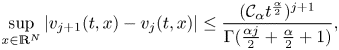 \begin{equation} \sup_{x \in \mathbb{R}^{N}} |v_{j+1}(t,x)- v_{j}(t,x)| \le \frac{ (\mathcal{C}_\alpha t^{\frac{\alpha}{2}})^{j+1}}{\Gamma (\frac{\alpha j}{2}+\frac{\alpha}{2}+1)} , \end{equation}
where  $\mathcal {C}_\alpha$ is given by
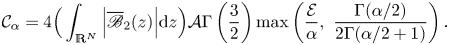 \begin{equation} \mathcal{C}_\alpha = 4 \Big( \int_{\mathbb{R}^{N}} \Big| \overline{\mathscr B}_2 (z) \Big|{\textrm{d}}z\Big) \mathcal{A} \Gamma \left( \frac{3}{2} \right) \max \left( \frac{\mathcal{E}}{\alpha},\ \frac{\Gamma(\alpha/2)}{2\Gamma(\alpha/2+1)} \right). \end{equation}
Indeed, for  $j=0$, using (4.12) and (4.13), we find that
 \begin{align*} \sup_{x \in \mathbb{R}^{N}} \Big|v_{1}(t,x)- v_{0}(t,x)\Big | &\le \Bigg\|\int_0^{t} \Delta \mathbb{K}_{2,\alpha} (t-\tau) F(v_{0}(\tau,x))\,{\textrm{d}}s\Bigg\|_{L^{\infty}}\\ &\le \int_0^{t} \| \Delta \mathbb{K}_{2,\alpha} (t-\tau,x) \|_{L^{1}(\mathbb{R}^{N})} \| F(v_{0}(\tau,x)) \|_{L^{\infty}} \,{\textrm{d}}\tau \\ &\le \frac{ 2 \mathcal{E}\Big( \int_{\mathbb{R}^{N}} \Big| \overline{\mathscr B}_2 (z) \Big|{\textrm{d}}z\Big) \mathcal{A} \Gamma \left( \frac{3}{2} \right)}{\Gamma \left( 1+\frac{\alpha}{2} \right)} \int_0^{t} (t-\tau)^{\alpha/2-1} \,{\textrm{d}}\tau\\ & = \frac{ 4 \mathcal{E} t^{\alpha/2}\Big( \int_{\mathbb{R}^{N}} \Big| \overline{\mathscr B}_2 (z) \Big|{\textrm{d}}z\Big) \mathcal{A} \Gamma \left( \frac{3}{2} \right)}{\alpha \Gamma \left( 1+\frac{\alpha}{2} \right)} \le \frac{t^{\alpha/2} \mathcal{C}_\alpha }{\Gamma(\alpha/2+1)} , \end{align*}
which means that (4.15) holds for  $j=0$. Suppose that (4.15) holds for
  $j \le n-1$, where
  $n \ge 2$ is a positive integer. From (4.8), we find that
 \begin{align} &\sup_{x \in \mathbb{R}^{N}} \Big|v_{n}(t,x)- v_{n-1}(t,x)\Big|\notag\\ &\quad \le \Bigg\|\int_0^{t} \Delta \mathbb{K}_{2,\alpha} (t-\tau) \Big( F(v_{n-1}(\tau,x)- F(v_{n-2}(s,x) \Big) \,{\textrm{d}}\tau \Bigg\|_{L^{\infty}}\nonumber\\ &\quad \le \int_0^{t} \Big\| \Delta \mathbb{K}_{2,\alpha} (t-\tau,x) \Big\|_{L^{1}(\mathbb{R}^{N})} \Big\| F(v_{n-1}(\tau,x)- F(v_{n-2}(\tau,x)\Big\|_{L^{\infty}} \,{\textrm{d}}\tau \nonumber\\ & \quad \le \frac{ 2 \mathcal{E}\Big( \int_{\mathbb{R}^{N}} \Big| \overline{\mathscr B}_2 (z) \Big|{\textrm{d}}z\Big) \mathcal{A} \Gamma \left( \frac{3}{2} \right)}{\Gamma \left( 1+\frac{\alpha}{2} \right)} \int_0^{t} (t-\tau)^{\alpha/2-1} \|v_{n-1}(\tau,.)- v_{n-2}(\tau,.)\|_{L^{\infty}} \,{\textrm{d}}\tau \nonumber\\ & \quad \le \frac{ 2 \mathcal{E}\Big( \int_{\mathbb{R}^{N}} \Big| \overline{\mathscr B}_2 (z) \Big|{\textrm{d}}z\Big) \mathcal{A} \Gamma \left( \frac{3}{2} \right)}{\Gamma \left( 1+\frac{\alpha}{2} \right)} \int_0^{t} \frac{ (t-\tau)^{\alpha/2-1} (\mathcal{C}_\alpha t^{\frac{\alpha}{2}})^{n-1}}{\Gamma (\frac{\alpha n}{2}-\frac{\alpha}{2}+1)} \,{\textrm{d}}\tau. \end{align}
Noting that  $\Gamma (\alpha ) \le 1$, we observe the following:
 \begin{align*} &\underline{The RHS of (4.17)}\\ &\quad = \frac{ 2 \mathcal{E}\Big( \int_{\mathbb{R}^{N}} \Big| \overline{\mathscr B}_2 (z) \Big|{\textrm{d}}z\Big) \mathcal{A} \Gamma \left( \frac{3}{2} \right)}{\Gamma \left( 1+\frac{\alpha}{2} \right)} \frac{ (\mathcal{C}_\alpha)^{n-1}}{\Gamma (\frac{\alpha n}{2}-\frac{\alpha}{2}+1)} \int_0^{t} (t-\tau)^{\alpha/2-1} \tau^{\frac{\alpha n-\alpha}{2}} \,{\textrm{d}}\tau \\ &\quad = \frac{ 2 \mathcal{E}\Big( \int_{\mathbb{R}^{N}} \Big| \overline{\mathscr B}_2 (z) \Big|{\textrm{d}}z\Big) \mathcal{A} \Gamma \left( \frac{3}{2} \right)}{\Gamma \left( 1+\frac{\alpha}{2} \right)} \frac{ (\mathcal{C}_\alpha)^{n-1}}{\Gamma (\frac{\alpha n}{2}-\frac{\alpha}{2}+1)} t^{\frac{\alpha n}{2}} \frac{\Gamma(\alpha/2)\Gamma(\frac{\alpha n-\alpha }{2}+1)}{\Gamma(\frac{\alpha n}{2}+1)}\\ & \quad \le \frac{ 2 \Gamma(\alpha/2) \mathcal{E}\Big( \int_{\mathbb{R}^{N}} \Big| \overline{\mathscr B}_2 (z) \Big|{\textrm{d}}z\Big) \mathcal{A} \Gamma \left( \frac{3}{2} \right)}{\Gamma \left( 1+\frac{\alpha}{2} \right)} \frac{ (\mathcal{C}_\alpha )^{n-1}}{\Gamma(\frac{\alpha n}{2}+1)} t^{\frac{\alpha n}{2}} \le \frac{ (\mathcal{C}_\alpha t^{\alpha/2} )^{n}}{\Gamma(\frac{\alpha n}{2}+1)} , \end{align*}
where in the last inequality, we have used from (4.16) that
 \[ \frac{ 2 \Gamma(\alpha/2) \mathcal{E}\Big( \int_{\mathbb{R}^{N}} \Big| \overline{\mathscr B}_2 (z) \Big|{\textrm{d}}z\Big) \mathcal{A} \Gamma \left( \frac{3}{2} \right)}{\Gamma \left( 1+\frac{\alpha}{2} \right)} \le \mathcal{C}_\alpha. \]
By the induction method, we derive that the estimate (4.15) holds for any  $j\ge 1.$ It follows from (4.15) that
 \begin{align} \left|\mkern-1.5mu\left|\mkern-1.5mu\left| {v_{j+1}-v_j} \right|\mkern-1.5mu\right|\mkern-1.5mu\right|_{\mathscr P_{ T_0}} &= \sup_{(t,x) \in \mathscr P_{ T_0} } \Big|v_{j+1}(t,x)- v_{j}(t,x)\Big|\notag\\ &\le \sup_{0 \le t \le T_0}\frac{ (\mathcal{C}_\alpha t^{\frac{\alpha}{2}})^{j+1}}{\Gamma (\frac{\alpha j}{2}+\frac{\alpha}{2}+1)} =\frac{ (\mathcal{C}_\alpha T_0^{\frac{\alpha}{2}})^{j+1}}{\Gamma (\frac{\alpha j}{2}+\frac{\alpha}{2}+1)}. \end{align}
Since (4.18), we deduce that for  $m> n$
 \begin{align} \left|\mkern-1.5mu\left|\mkern-1.5mu\left| {v_{m}-v_n} \right|\mkern-1.5mu\right|\mkern-1.5mu\right|_{\mathscr P_{ T_0}} &= \sup_{(t,x) \in \mathscr P_{ T_0} } \Big|v_{m}(t,x)- v_{n}(t,x)\Big|\le \sum_{j=n}^{m} \big\|v_{j+1}(t,x)- v_{j}(t,x)\big\|_{L^{\infty}}\notag\\ &\le \sum_{j=n}^{m} \frac{ (\mathcal{C}_\alpha T_0^{\frac{\alpha}{2}})^{j+1}}{\Gamma (\frac{\alpha j}{2}+\frac{\alpha}{2}+1)} . \end{align}
In the next step, we claim that the infinite sum  $\sum _{j=1}^{\infty } \frac { (\mathcal {C}_\alpha T_0^{\frac {\alpha }{2}})^{j+1}}{\Gamma (\frac {\alpha j}{2}+\frac {\alpha }{2}+1)}$ is convergent. Due to the definition of
  $T_0$ as in (4.5), we find that
  $T_0^{\alpha /2} \le \frac {\alpha \Gamma (\alpha /2+1)} {4( \int _{\mathbb {R}^{N}} | \overline {\mathscr B}_2 (z) |{\textrm {d}}z) \mathcal {A} \Gamma ( \frac {3}{2} )\Gamma (\alpha /2) } .$ By relying on (4.16), we can easily achieve that
 \[ (\mathcal{C}_\alpha T_0^{\alpha/2})^{j+1} \le \left( 4 \Big( \int_{\mathbb{R}^{N}} \Big| \overline{\mathscr B}_2 (z) \Big|{\textrm{d}}z\Big) \mathcal{A} \Gamma \left( \frac{3}{2} \right) \frac{\Gamma(\alpha/2)}{2\Gamma(\alpha/2+1)} T_0^{\alpha/2} \right)^{j+1} \le \left( \frac{\alpha}{2} \right)^{j+1}. \]
Since  $\alpha >1/2$, we know that
  $\alpha j+\alpha +1 >2$ for
  $j \ge 1$. Due to the fact that the function
  $\Gamma (z)$ is increasing for
  $z>2$, we find that
  $\Gamma (\alpha j+\alpha +1) > \Gamma (2\alpha +1)$. It follows from (4.20) that for
  $m > n \ge \overline {M}$
 \begin{align*} \big\|v_{m}(t,x)- v_{n}(t,x)\big\|_{L^{\infty}} &\le \frac{1}{\Gamma (2\alpha+1)} \sum_{j=n}^{m} \left( \frac{\alpha}{2} \right)^{j+1}\le \frac{1}{\Gamma (2\alpha+1)} \sum_{j=\overline{M}}^{\infty} \left( \frac{\alpha}{2} \right)^{j+1} \\ &\le \frac{2}{(2-\alpha) \Gamma (2\alpha+1)}\left(\frac{\alpha}{2} \right)^{\overline{M}+1}. \end{align*}
Now, given any  $\epsilon >0$, we can pick
  $\overline {M}$, depending on
  $\epsilon$, such that
  $\frac {2}{(2-\alpha ) \Gamma (2\alpha +1)}(\frac {\alpha }{2} )^{\overline {M}+1} < \epsilon .$ Some of above observations allow us to conclude that the sequence
  $\{v_n\}$ is a Cauchy one in the space
  $L^{\infty }(\mathbb {R}^{N})$. Therefore, there exists a function
  $v(t,x)$ which is the limitation of the sequence
  $\{v_n\}$ on the strip
  $\mathscr P_{ T_0}$. It is obvious to see that
  $v$ is a continuous solution of the integral equation (4.6) on the strip
  $\mathscr P_{ T_0}$. Next, we examine the regularity of the solution
  $u$. We only need to derive the following estimation. For each
  $1\le k \le L,\ n \ge 1$, there exists
  $\mathscr Q_k$ which is a continuous increasing function of
  $t-t_k$ such that, for each
  $0< t_1 < t_2<\cdots < t_N < t \le T_0$, the following estimate holds true
 \[ \|D^{k} v_n(t,x)\|_{L^{\infty}} \le (t-t_k)^{-\frac{\alpha k}{4}} \mathcal{Q}_k (\mathcal{E}, \alpha, t_k-t_1, t-t_k), \quad t_k < t \le T_0. \]
From formula (4.8), we find that
 \begin{align} D v_n(t,x)&= D \mathbb{Z}_{1,\alpha} (t- t_1) v_n (t_1, x)\notag\\ &\quad + \int_{t_1}^{t} D^{3} \mathbb{Z}_{2,\alpha} (t-\tau) F(v_{n-1}(\tau,x))\,{\textrm{d}} \tau,\quad t_1 \le t \le T_0. \end{align}
This implies that
 \begin{align} \sup_{x \in \mathbb{R}^{N} } \Big| D v_{n}(t,x)\Big|&\le \sup_{x \in \mathbb{R}^{N} } \Big| D \mathbb{Z}_{1,\alpha} (t- t_1) v_n (t_1, x) \Big|\notag\\ &\quad + \sup_{x \in \mathbb{R}^{N} } \Bigg| \int_{t_1}^{t} D^{3} \mathbb{Z}_{2,\alpha} (t-\tau) F(v_{n-1}(\tau,x))\,{\textrm{d}} \tau \Bigg| \nonumber\\ &=\underbrace{ \sup_{x \in \mathbb{R}^{N} } \Big| D \Big(\mathbb{K}_{1,\alpha} (t-t_1,x) * v_n(t_1,x) \Big) \Big|}_{(I)}\notag\\ &\quad + \underbrace{ \sup_{x \in \mathbb{R}^{N} } \int_{t_1}^{t} \left| D^{3} \mathbb{Z}_{2,\alpha} (t-\tau) F(v_{n-1}(\tau,x)) \right| \,{\textrm{d}}\tau}_{(II)}. \end{align}
Using the fact that  $\frac {{\textrm {d}}}{{\textrm {d}}x} (f(x)*g(x) )= ( \frac {{\textrm {d}}}{{\textrm {d}}x}f(x) )* g(x)$ and thanks to lemma (2.3), the term
  $(I)$ is bounded by
 \begin{align} (I)&= \sup_{x \in \mathbb{R}^{N} } \Big| D \Big(\mathbb{K}_{1,\alpha} (t-t_1,x) * v_n(t_1,x) \Big) \Big| = \Big\| D \mathbb{K}_{1,\alpha} (t-t_1, .) * v_n(t_1,.) \Big\|_{L^{\infty}} \nonumber\\ &\le \| D \mathbb{K}_{1,\alpha} (t-t_1, .) \|_{L^{1}(\mathbb{R}^{N})} \| v_n(t_1,.) \|_{L^{\infty}}\le 2 \mathcal{E} \mathscr C_{1,1} (\alpha, N) (t-t_1)^{-\frac{\alpha }{4}} \end{align}
Using (4.4) and the second part of lemma (2.3) with  $p=1, k=3$, we find that the term
  $(II)$ is bounded by
 \begin{align} (II) &\le \int_{t_1}^{t} \left\| D^{3} \mathbb{Z}_{2,\alpha} (t-\tau) F(v_{n-1}(\tau,x)) \right\|_{L^{\infty}} \,{\textrm{d}}\tau\nonumber\\ &\le \int_{t_1}^{t} \big\| D^{3} \mathbb{K}_{2,\alpha} (t-\tau,.) \big\|_{L^{1}(\mathbb{R}^{N})} \| F(v_{n-1}(\tau,.)) \|_{L^{\infty}} \,{\textrm{d}}\tau \nonumber\\ &\le \mathcal{A} \sup_{(t,x) \in [0, T_0] \times \mathbb{R}^{N} } |v_{n-1}(t,x)| \int_{t_1}^{t} \Big\| D^{3} \mathbb{K}_{2,\alpha} (t-\tau,.) \Big\|_{L^{1}(\mathbb{R}^{N})} \,{\textrm{d}}\tau\nonumber\\ &\le 2 \mathcal{E} \mathcal{A} \overline{ \mathscr C_{3,1}} (\alpha, N) \int_{t_1}^{t} (t-\tau)^{\alpha-\frac{\alpha N}{4}-1+\frac{\alpha N}{4}-\frac{3\alpha }{4}} \,{\textrm{d}}\tau= \frac{ 8\mathcal{E} \mathcal{A} \overline{ \mathscr C_{3,1}} (\alpha, N) }{\alpha} (t-t_1)^{\frac{\alpha}{4}}. \end{align}
Combining (4.21), (4.22) and (4.23), we deduce that there exists  $\mathscr Q_1$ which is a continuous increasing function of
  $t-t_1$ such that
 \begin{equation} \sup_{x \in \mathbb{R}^{N} } \Big| D v_{n}(t,x)\Big| \le (t-t_1)^{\frac{-\alpha}{4}} \mathscr Q_1 (\mathcal{E}, \alpha, t-t_1). \end{equation}
From formula (4.8), we find that
 \begin{align} D^{2} v_n(t,x)&= D^{2} \mathbb{Z}_{1,\alpha} (t- t_2) v_n (t_1, x)\notag\\ &\quad + \int_{t_2}^{t} D^{4} \mathbb{Z}_{2,\alpha} (t-\tau) F(v_{n-1}(\tau,x))\,{\textrm{d}} \tau,\quad t_2 \le t \le T_0. \end{align}
By a similar argument as above, we find that
 \begin{align} \sup_{x \in \mathbb{R}^{N} } \Big| D^{2} v_{n}(t,x)\Big|&\le \sup_{x \in \mathbb{R}^{N} } \Big| D^{2} \mathbb{Z}_{1,\alpha} (t- t_2) v_n (t_2, x) \Big|\notag\\ &\quad + \sup_{x \in \mathbb{R}^{N} } \Bigg| \int_{t_2}^{t} D^{4} \mathbb{Z}_{2,\alpha} (t-\tau) F(v_{n-1}(\tau,x))\,{\textrm{d}} \tau \Bigg| \nonumber\\ & \le \Big\| D^{2} \mathbb{K}_{1,\alpha} (t-t_2, .) \Big\|_{L^{1}(\mathbb{R}^{N})} \| v_n(t_2,.) \|_{L^{\infty}} \nonumber\\ &\quad+ \int_{t_2}^{t} \big\| D^{3} \mathbb{K}_{2,\alpha} (t-\tau,.) \big\|_{L^{1}(\mathbb{R}^{N})} \| DF(v_{n-1}(\tau,.)) \|_{L^{\infty}} \,{\textrm{d}}\tau \nonumber\\ &\le 2 \mathcal{E} \mathscr C_{2,1} (\alpha, N) (t-t_2)^{-\frac{\alpha }{2}} + (12 \mathcal{E}^{2}+1) \overline{ \mathscr C_{3,1}} (\alpha, N) \nonumber\\ &\quad \times \int_{t_2}^{t} \mathscr Q_1 (\mathcal{E}, \alpha, \tau -t_1) (\tau -t_1)^{\frac{-\alpha}{4}} (t-\tau)^{\frac{\alpha}{4}-1} \,{\textrm{d}}\tau,\end{align}
where it follows from (4.24) that
 \begin{align*} \big\| DF(v_{n-1}(\tau,.)) \big\|_{L^{\infty}} &\le \|3 v_{n-1}^{2}-1\|_{L^{\infty}} \| D(v_{n-1}(\tau,.)) \|_{L^{\infty}}\\ &\le (12 \mathcal{E}^{2}+1) (\tau -t_1)^{\frac{-\alpha}{4}} \mathscr Q_1 (\mathcal{E}, \alpha, \tau -t_1). \end{align*}
Now, we handle the integral term on the RHS of expression (4.26). It is noted that  $(\tau -t_1)^{\frac {-\alpha }{4}} \le (t_2 -t_1)^{\frac {-\alpha }{4}}$ for any
  $\tau \ge t_2$, and we find that
 \begin{align*} &\int_{t_2}^{t} \mathscr Q_1 (\mathcal{E}, \alpha, \tau -t_1) (\tau -t_1)^{\frac{-\alpha}{4}} (t-\tau)^{\frac{\alpha}{4}-1} \,{\textrm{d}}\tau\\ &\quad \le \mathscr Q_1 (\mathcal{E}, \alpha, t_2 -t_1)(t_2 -t_1)^{\frac{-\alpha}{4}} \int_{t_2}^{t} (t-\tau)^{\frac{\alpha}{4}-1} \,{\textrm{d}}\tau \end{align*}
where we recall that  $\mathscr Q_1$ is a continuous increasing function of
  $t-t_1$. Therefore, it follows from the latter above estimate that
 \begin{align} &\int_{t_2}^{t} \mathscr Q_1 (\mathcal{E}, \alpha, \tau -t_1) (\tau -t_1)^{\frac{-\alpha}{4}} (t-\tau)^{\frac{\alpha}{4}-1} \,{\textrm{d}}\tau\notag\\ &\quad \le \frac{4\mathscr Q_1 (\mathcal{E}, \alpha, t_2 -t_1)(t_2 -t_1)^{\frac{-\alpha}{4}} }{\alpha } (t-t_2)^{\alpha/4}. \end{align}
Combining (4.26) and (4.27), we arrive at
 \[ \sup_{x \in \mathbb{R}^{N} } \Big| D^{2} v_{n}(t,x)\Big| \le \mathscr Q_2 (\mathcal{E}, \alpha, t_2 -t_1, t-t_2) (t-t_2)^{-\frac{\alpha }{2}}, \]
where
 \begin{align*} &\mathscr Q_2 (\mathcal{E}, \alpha, t_2 -t_1, t-t_2) =2 \mathcal{E} \mathscr C_{2,1} (\alpha, N)\\ &\quad + \frac{4\mathscr Q_1 (\mathcal{E}, \alpha, t_2 -t_1)(t_2 -t_1)^{\frac{-\alpha}{4}} }{\alpha } (t-t_2)^{3\alpha/4}. \end{align*}
It is easy to verify that  $\mathscr Q_2$ as above is a continuous increasing function of
  $t-t_2$. By a similar way as above, we can verify that
  $\mathscr Q_k$ as above is a continuous increasing function of
  $t-t_k$ for any
  $k$ is a natural number such that
  $k \ge 2$. This completes our proof.
Appendix A.
Definition A.1 Let  $\alpha$ be a complex number whose real part is positive. The Gamma function can be formulated as
  $\Gamma (\alpha )=\int _{0}^{\infty }\frac {x^{\alpha -1}}{{\textrm {e}}^{x}}\,{\textrm {d}}x,$ and the M-Wright type function
  $\mathcal {M}_{\alpha }$ is given by
  $\mathcal {M}_{\alpha }(z)=\sum _{j=1}^{\infty }\frac {(-z)^{m}}{m!\Gamma \left [{-\alpha m+(1-\alpha )}\right ]}$.
Lemma A.2 (see [Reference de Carvalho-Neto and Planas13, proposition 2] or [Reference Mainardi31, Appendix F])
Let  $\alpha \in (0,1)$ and
  $\theta >-1$. Then, the following properties holds
 \begin{equation} \mathcal{M}_\alpha(\nu) \ge 0,\quad \forall\, \nu \ge 0, \quad \textrm{and} \quad \int_0^{\infty} \nu^{\theta} \mathcal{M}_\alpha(\nu) {\textrm{d}}\nu = \frac{\Gamma(\theta+1)}{\Gamma(\theta\alpha+1)},\quad \forall\, \theta>{-}1.\end{equation}
Proposition A.1 Let  $a,b>0$ and
  $q\ge 1$. Then the following inequality holds
 \[ (a+b)^{p}\le 2^{q-1}\left(a^{q}+b^{q}\right). \]
Proof. From the fact that  $q(q-1)x^{q-2}\ge 0$ for any
  $x>0$ and
  $q\ge 1$, we assert that the one variable function
  $f(x)=x^{q}, q>0$ is a convex function. It follows that
 \[ f\left(\frac{\sum_{k=1}^{M}a_k}{M}\right)\le\frac{\sum_{k=1}^{M}f(a_k)}{M}. \]
This one gives us the desired result.
Lemma A.3 (Young's convolution inequality) Let  $p,q,r\in [1,\infty ]$ such that
 \[ 1+\frac{1}{r}=\frac{1}{p}+\frac{1}{q}. \]
Then, the inequality  $\left \| {u*v} \right \|_{L^{r}}\le \left \| {u} \right \|_{L^{p}}\left \| {v} \right \|_{L^{q}}$ holds for every
  $u\in {L^{p}(\mathbb {R}^{N})}$ and
  $v\in {L^{q}(\mathbb {R}^{N})}$.
Lemma A.4 (fractional Grönwall inequality) Let  $m,n$ be positive constants and
  $\zeta \in (0,1).$ Assume that function
  ${u}\in L^{\infty ,*}(0,T]$ satisfies the following inequality
 \[ {u}(t)\le m+n\int_{0}^{t}(t-\tau)^{\zeta-1}{u}(r){\textrm{d}}r,\quad\text{for all}\ t\in(0,T], \]
then, the result below is satisfied
 \[ {u}(t)\le mE_{\zeta,1}\left({n\Gamma(\zeta)t^{\zeta}}\right). \]
Acknowledgments
The authors would like to thank the anonymous referees for their valuable comments leading to the improvement of our manuscript. This work was supported by Vietnam National Foundation for Science and Technology Development (NAFOSTED) under grant number 101.02-2019.09. The research of T. C. has been partially supported by the Spanish Ministerio de Ciencia, Innovación y Universidades (MCIU), Agencia Estatal de Investigación (AEI) and Fondo Europeo de Desarrollo Regional (FEDER) under the project PGC2018-096540-B-I00, and by Junta de Andalucía (Consejería de Economía y Conocimiento) and FEDER under projects US-1254251 and P18-FR-4509.


