2 Direct numerical simulations

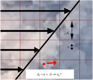
The DNS of a turbulent flow with small heavy particles is carried out in a confined periodic cubic box of size $L=2\unicode[STIX]{x03C0}$ discretized on $N^{3}=512^{3}$ grid points, and with a uniform mean shear $S$ imposed in one spatial direction. The mean velocity field $\boldsymbol{U}(x_{1},x_{2},x_{3})=(Sx_{2},0,0)$ is sketched in figure 1(a). The advection in the $x_{2}$ direction by the mean shear is incoherent with the periodic boundary conditions specified for the Navier–Stokes equations in this direction. In order to circumvent this problem, we follow the proposal in Rogallo (Reference Rogallo1981) to carry out the simulation in a mesh moving with the mean velocity frame: $x_{1}^{\prime }=x_{1}-Sx_{2}t$; $x_{2}^{\prime }=x_{2}$; $x_{3}^{\prime }=x_{3}$. The computational box is preserved from increasing distortion by using a remeshing procedure. In Sekimoto et al. (Reference Sekimoto, Dong and Jimenez2016), it has been shown that the typical configuration of homogeneous shear flow (stretched streamwise vortical streaks, ‘minimal’ in size in the spanwise direction) suggests, for statistical stationarity, the spanwise box width $L_{z}$ to be the main limit for setting the length and velocity scales, with the two other box dimensions larger than the box width. On the other hand, with increasing aspect ratio, the errors induced by remeshing the solutions may be also increased in prediction of the small-scale properties of the flow (Pumir Reference Pumir1996), particularly when the mesh is getting coarser, as for LES with $32^{3}$ grid points, for example. In our simulation, the geometry is indeed too short for the longitudinal velocity to become independent of the box length but the spanwise integral length scale is less than the box dimension ($L_{z}/L\sim 0.19$), and since the main objective of our DNS and LES is to produce a background flow, with the emphasis on the response of particles loaded in that presumed flow, the assumed statistical stationarity in our simulation is based on an aspect ratio equal to 1. It is also seen in Sekimoto et al. (Reference Sekimoto, Dong and Jimenez2016) that the bursting event period in a cubic box is similar to the period in an optimal geometry. Besides, the numerical method has been assessed by the good prediction (not shown in the manuscript) of Eulerian (three components of the kinetic energy, the anisotropy tensor, integral length) and Lagrangian (the fluid particle acceleration) statistics reported in Rogallo (Reference Rogallo1981), Rogers & Moin (Reference Rogers and Moin1987) and Yeung (Reference Yeung1997). In the moving frame (hereafter we remove primes from the coordinate notation), the Navier–Stokes equations for the fluctuating field are

(2.1)$$\begin{eqnarray}\displaystyle & \displaystyle {\displaystyle \frac{\unicode[STIX]{x2202}u_{i}}{\unicode[STIX]{x2202}t}}+{\displaystyle \frac{\unicode[STIX]{x2202}u_{i}u_{j}}{\unicode[STIX]{x2202}x_{j}}}+Su_{2}\unicode[STIX]{x1D6FF}_{i1}=-{\displaystyle \frac{1}{\unicode[STIX]{x1D70C}}}{\displaystyle \frac{\unicode[STIX]{x2202}p}{\unicode[STIX]{x2202}x_{i}}}+\unicode[STIX]{x1D708}{\displaystyle \frac{\unicode[STIX]{x2202}u_{i}}{\unicode[STIX]{x2202}x_{j}\unicode[STIX]{x2202}x_{j}}}, & \displaystyle\end{eqnarray}$$

(2.2)$$\begin{eqnarray}\displaystyle & \displaystyle {\displaystyle \frac{\unicode[STIX]{x2202}u_{i}}{\unicode[STIX]{x2202}x_{i}}}=0. & \displaystyle\end{eqnarray}$$

These equations are solved by pseudo-spectral methods in space; the nonlinear terms are directly solved with the classical $2/3$ rule in order to avoid aliasing errors, and the linear terms are implicitly calculated. The time integration scheme is based on the second-order Runge–Kutta scheme. The shear parameter $S^{\ast }=Sk/\unicode[STIX]{x1D716}$, with $k=\langle u_{i}u_{i}\rangle /2$, which characterizes the measure of the strength of the shear relative to the turbulence time scale, has been used in many studies of homogeneous shear flow. The question as to whether or not the long term asymptotics of the homogeneous shear flow are sensitive to the choice of the initial value of this parameter is addressed in Isaza & Collins (Reference Isaza and Collins2009). Using different DNS, which yielded mixed results in response to this question, Isaza & Collins (Reference Isaza and Collins2009) have demonstrated such sensitivity, and particularly in the temporal evolution of the shear parameter itself. However, that study was performed for relatively short-time behaviour of the homogeneous shear flow ($S\cdot t<8$), and not for long times $S\cdot t$ when the statistically stationary state is attained. We performed simulations with different initial values of the shear parameter by varying both the uniform mean shear $S$ and the kinematic viscosity $\unicode[STIX]{x1D708}$, up to the statistically stationary state $S\cdot t=100$. The latter, characterized by a succession of spikes in the total turbulent kinetic energy, is defined on the bases of the time averaged parameters, such as the integral length scale, the total kinetic energy, the total dissipation rate, the Reynolds number and the Kolmogorov length. If those parameters are not varying with time, the state is referred to as statistically stationary. The initial condition is a random homogeneous isotropic velocity field generated at the prescribed Reynolds number. The evolution of $S^{\ast }$ for each case is shown in figure 1(b). It is seen that, at early times, the evolution of the shear parameter is sensitive to its initial value choice, as in Isaza & Collins (Reference Isaza and Collins2009). When the flow reaches the statistically stationary state, the shear parameter is likely to lose such sensitivity. In this study, we define the homogeneous shear $S$ as the main parameter and not the initial value of the shear parameter $S^{\ast }$. The parameters we use are $S=3.2~\text{s}^{-1}$ and $\unicode[STIX]{x1D708}=0.005~\text{m}^{2}~\text{s}^{-1}$. The inertial particles are injected when the flow reaches the statistically stationary state. The latter is characterized by the following parameters, averaged in time: the integral scale $L_{int}=3.96~\text{m}$, the shear length scale $L_{S}=0.66~\text{m}$, the Kolmogorov scale $\unicode[STIX]{x1D702}=0.00961~\text{m}$, the integral time scale $T_{int}=0.55~\text{s}$, the Kolmogorov time $\unicode[STIX]{x1D70F}_{\unicode[STIX]{x1D702}}=0.0185~\text{s}$, the viscous dissipation $\langle \unicode[STIX]{x1D716}\rangle =14.6~\text{m}^{2}~\text{s}^{-3}$ and the Reynolds number $Re_{\unicode[STIX]{x1D706}}=2k\sqrt{5/(3\langle \unicode[STIX]{x1D716}\rangle \unicode[STIX]{x1D708})}=164$. We measured the quality of our resolution by ensuring that $\unicode[STIX]{x1D705}_{max}\unicode[STIX]{x1D702}\geqslant 1$, as is commonly done in the literature (Pumir Reference Pumir1996; Gualtieri et al. Reference Gualtieri, Casciola, Benzi, Amati and Piva2002). Here, $\unicode[STIX]{x1D705}_{max}\unicode[STIX]{x1D702}=2.3$ with $\unicode[STIX]{x1D705}_{max}\approx \sqrt{2}N/3$. In Isaza & Collins (Reference Isaza and Collins2009) it is recommended also that $L_{11}/L\leqslant 0.1$ to properly resolve the large scales. This condition is difficult to fulfil in the homogeneous shear flow at the statistically stationary state since the integral values are confined by the size of the box. Therefore, to gauge our resolution, we required $\unicode[STIX]{x1D705}_{max}\unicode[STIX]{x1D702}\geqslant 1$. Assuming the Stokes drag to be the only force acting on the particle, the particle motion equations are

(2.3)$$\begin{eqnarray}\displaystyle & \displaystyle {\displaystyle \frac{\text{d}x_{pi}}{\text{d}t}}=u_{pi}(t)+\unicode[STIX]{x1D6FF}_{i1}Sx_{p2}(t), & \displaystyle\end{eqnarray}$$

(2.4)$$\begin{eqnarray}\displaystyle & \displaystyle {\displaystyle \frac{\text{d}u_{pi}}{\text{d}t}}={\displaystyle \frac{u_{i}(x_{pi}(t),t)-u_{pi}(t)}{\unicode[STIX]{x1D70F}_{p}}}+\unicode[STIX]{x1D6FF}_{i1}Su_{p2}(t). & \displaystyle\end{eqnarray}$$

Here, $u_{pi}(t)$ is the particle velocity, $u_{i}(x_{pi}(t),t)$ is the fluid velocity at the particle position and $\unicode[STIX]{x1D70F}_{p}=(\unicode[STIX]{x1D70C}_{p}d_{p}^{2})/18\unicode[STIX]{x1D70C}\unicode[STIX]{x1D708}$ is the typical response time of the particles. The interpolation of the fluid velocity to the particle position is done using the interpolation kernel described in Lagaert, Balarac & Cottet (Reference Lagaert, Balarac and Cottet2014) which is of order 4 in space; details may be found also in Cottet et al. (Reference Cottet, Etancelin, Perignon and Picard2014). Henceforth, the Stokes number is defined as $St=\unicode[STIX]{x1D70F}_{p}/\unicode[STIX]{x1D70F}_{\unicode[STIX]{x1D702}}$. In simulations, we consider the flow seeded by either infinitesimal tracers, or inertial particles, these are characterized by $St=0.3$ (small particles) and $St=3.0$ (large particles). As is seen from (2.4), the mean acceleration in the streamwise direction is defined by $Su_{p2}$. It has been shown in Yeung (Reference Yeung1997) that the latter makes a negligible contribution to the particle dynamics. Therefore, we consider the fluctuating components of the acceleration only, denoted hereafter by $a_{1},a_{2}$ and $a_{3}$. The remeshing step in the algorithm from Rogallo (Reference Rogallo1981) is known to create losses of the total kinetic energy and dissipation rate. To minimize the impact of this feature on the particle statistics, we applied a time-filtering operation on the particle velocity signal with a filter width chosen to be lower than the Kolmogorov time. The particle acceleration is then recomputed by the derivative of the velocity signal. Oscillations of the particle acceleration statistics due to the remeshing step may be seen in figure 6(a). However, these variations are small in comparison with global variations of the acceleration. Moreover, with increasing Stokes number, these oscillations are substantially decreased. The statistics sampled on time windows without remeshing did not show significant differences with the statistics computed on the whole simulation. In the next section, the DNS statistics accumulated for all computed particles at the statistically stationary state are presented.

Figure 2. (a) Longitudinal acceleration PDF of fluid particles (– – –) and solid particles ($St=0.3$: $\cdots \cdots$; $St=3.0$: ——) in the homogeneous shear flow. The PDFs are standardized by $a_{rms}=\langle a^{2}\rangle ^{1/2}$. (b) PDFs of the acceleration norm of fluid and solid particles compared to the log-normal distribution (●) with the following parameters: $\unicode[STIX]{x1D707}=-\ln 2/2$, $\unicode[STIX]{x1D70E}=\ln 2$. PDFs are standardized by $a_{rms}=\langle a^{2}\rangle ^{1/2}$.

3 Statistics of the particle acceleration in homogeneous shear flow

With increasing particle inertia, the impact of intense acceleration events in the fluid on the particle motion is filtered. In HIT, this is illustrated, for example in Bec et al. (Reference Bec, Biferale, Boffetta, Celani, Cencini, Lanotte, Musacchio and Toschi2006) and Sabelnikov et al. (Reference Sabelnikov, Barge and Gorokhovski2019). The illustration of this effect in the case of homogeneous shear flow is given in figure 2(a). While the particle acceleration probability density function (PDF) for the fluid particle and for the particle with relatively low inertia, $St=0.3$, exhibit stretched tails, these are significantly reduced if the Stokes number is increased up to $St=3.0$. The same conclusion holds for the PDF of the acceleration norm $|a|=(a_{i}a_{i})^{1/2}$, as is shown in figure 2(b). Surprisingly, in the case of fluid and small inertial particles (addressed here to $St=0.3$), the ratio of the acceleration norm to its root mean square (the subscript rms) $\unicode[STIX]{x1D709}=|a|/a_{rms}$, $a_{rms}=\langle a^{2}\rangle ^{1/2}$ follows fairly well the log-normal distribution expressed by $LN(\unicode[STIX]{x1D709},\unicode[STIX]{x1D707},\unicode[STIX]{x1D70E}^{2})=1/\unicode[STIX]{x1D709}\unicode[STIX]{x1D70E}^{2}\sqrt{2\unicode[STIX]{x03C0}}\exp (-((\ln \unicode[STIX]{x1D709}-\unicode[STIX]{x1D707})^{2})/2\unicode[STIX]{x1D70E}^{2})$, with the presumed mean $\unicode[STIX]{x1D707}=-\ln 2/2$ and standard deviation $\unicode[STIX]{x1D70E}^{2}=\ln 2$. Here, the angled brackets denote the average over all particles in the statistically stationary flow. Using the expression for the moments of the log-normal distribution $m_{k}=\exp (k\unicode[STIX]{x1D707}+k^{2}\unicode[STIX]{x1D70E}^{2}/2)$, as shown in Zamansky et al. (Reference Zamansky, Vinkovic and Gorokhovski2013), the mentioned values of parameters $\unicode[STIX]{x1D707}$ and $\unicode[STIX]{x1D70E}$ correspond to the following condition for the acceleration norm: $\langle |a|^{2}\rangle ^{1/2}=\langle |a|\rangle$. The occurrence of such a high level of fluctuations of the particle acceleration components in highly turbulent conditions is discussed in Chen et al. (Reference Chen, Coleman, Vassilicos and Hu2010). Remarkably also is that the log-normality of the particle acceleration norm persists for different ‘latitude’ angles $\unicode[STIX]{x1D703}$ (indicated in figure 3(a)) of the particle acceleration direction. In figure 3(b,c), it is seen that the distributions of the acceleration norm of the fluid particle, and of the small inertial particle as well, preserve the same shape independently of the ‘latitude’ $\unicode[STIX]{x1D703}$; these distributions follow fairly well the unconditional PDF, which is log-normal. As seen in figure 3(d), the norm of the large inertial particle, $St=3.0$, preserves also the statistical independence of its orientation. The same results (not demonstrated here) are obtained for varying the ‘longitude’ $\unicode[STIX]{x1D719}$. We conclude that, in the statistically stationary homogeneous shear flow, the amplitude and the direction of the Lagrangian acceleration behave as two almost statistically independent variables. The same conclusion was also drawn for inertial particles in HIT (Pope Reference Pope1990; Mordant et al. Reference Mordant, Deloura, Leveque, Arneodo and Pinton2002; Sabelnikov et al. Reference Sabelnikov, Barge and Gorokhovski2019) and channel flows (Zamansky et al. Reference Zamansky, Vinkovic and Gorokhovski2013). This implies a large separation in time scales for autocorrelation functions corresponding to the fluctuating parts of the particle acceleration and its amplitude. The demonstration for the fluid particle and for the particle with $St=0.3$, as well as for the angle $\unicode[STIX]{x1D703}$, is given in figure 4. The corresponding correlation times, $T_{|a|}$ and $T_{a}$, and the Kolmogorov time $\unicode[STIX]{x1D70F}_{\unicode[STIX]{x1D702}}$, are also presented in this figure. It is seen that, although both correlation times $T_{a}$ for $St=0.3$ and $St=3.0$ remain of the order of the Kolmogorov time, the correlation time $T_{a}$ is increased when the Stokes number is increased: the direction of the heavier particle, being changed by helical structures, persists for a longer time. As to the amplitude of the particle acceleration, it correlates to much longer times than the acceleration direction, and the correlation time $T_{|a|}$ is decreased when the Stokes number is increased: the particle response to the short-lived intense perturbations of the fluid has a lesser magnitude for a heavier particle, and thereby that magnitude is probably less correlated (Jung, Yeo & Lee Reference Jung, Yeo and Lee2008). It is also seen that, with increasing Stokes number, the particle acceleration component in the downstream direction is correlated on longer times in comparison with the two other components, suggesting that the effect of the particle entrainment by longitudinal vortical structures is enhanced with increasing particle inertia. We will return to this effect later on. The long-time correlation of the particle acceleration norm suggests that its statistics may be linked with the properties of the large-scale structure fluctuations, as it takes place in the regeneration cycle in homogeneous shear flow. The spectral energy balance, performed in Barge & Gorokhovski (Reference Barge and Gorokhovski2019) conditionally on periods of increase and decrease of the total kinetic energy, shows that the energy transfer down to smaller scales is different for these periods, and the difference is attributed to scales larger than the shear length scale $L_{S}$. Consequently, one can expect also a sensitivity of the acceleration norm to the regenerating cycle.

Figure 3. (a) Definition of the angles and the acceleration components. (b) Distribution of the fluid particle acceleration norm conditioned to different values of the angle $\unicode[STIX]{x1D703}$ ($\cdots \cdots$ from light to dark grey: $\unicode[STIX]{x1D703}=-3\unicode[STIX]{x03C0}/8,-\unicode[STIX]{x03C0}/4,-\unicode[STIX]{x03C0}/8,0,\unicode[STIX]{x03C0}/8,\unicode[STIX]{x03C0}/4,3\unicode[STIX]{x03C0}/8$) and compared with the unconditioned distribution (●) to the angle $\unicode[STIX]{x1D703}$. (c) Same for the small inertial particle, $St=0.3$. (d) Same for the large inertial particle, $St=3.0$.

Figure 4. (a) Autocorrelation functions of the norm $|a|$ (●), components ($a_{1}$, ▿; $a_{2}$, $\times$; $a_{3}$, ♦) and the orientation angle $\unicode[STIX]{x1D703}=\arctan (a_{2}/a_{1})$ (— ⋅ ⋅ —) of the acceleration vector of fluid particles. (b) Same for the large particles, $St=3.0$. Here $T_{|a|}$ is the correlation time of the particle acceleration norm, $T_{a}$ is the correlation time of the particle acceleration and $\unicode[STIX]{x1D70F}_{\unicode[STIX]{x1D702}}$ is the Kolmogorov time.

Figure 5. (a) Autocorrelation functions of the acceleration norm $|a|$ of fluid particles in the homogeneous shear flow averaged over the complete simulation (——) and conditioned to the growth phase (– – –) and to the collapse phase (●). (b) Same for inertial particle with $St=3.0$. Here $T_{|a|}$ is the correlation time of the particle acceleration norm, subscripts ‘$G$’ and ‘$C$’ denote the conditioning to the growth and collapse phases, respectively.

Figure 6. Succession of spikes in the standard deviation $\langle |a|^{2}\rangle ^{1/2}$ (——) and in the mean $\langle |a|\rangle$ (●) of the acceleration norm of all particles at the given moment; these values are non-dimensionalized by averaged $\langle |a|\rangle _{t}$, over the full time. The Eulerian Reynolds stress $\langle u_{1}u_{2}\rangle /\langle u_{1}u_{2}\rangle _{t}$ (– – –) is plotted also to see the correlation between the Eulerian statistics and the periodic character of the particle acceleration due to the bursting events in the flow. (a) Fluid particle. (b) $St=0.3$. (c) $St=3.0$.

Figure 7. (a) The PDF of the angle of the Lagrangian acceleration vector projected in plane $x_{1}$, $x_{2}$ (upper curves) and $x_{1}$, $x_{3}$ (lower curves), fluid particles (– – –); solid particles ($St=0.3$, $\cdots \cdots$; $St=3.0$, ——). (b) Evolution of the correlation coefficient between the orientation of the fluid particle acceleration and the orientation of the vorticity vector ‘seen’ by the particles as a function of block sizes. (c) Block pictures PDF of the $\unicode[STIX]{x1D703}$ angle for fluid particles and for different block sizes ($5\unicode[STIX]{x1D702}$, $-\cdot -$; $10\unicode[STIX]{x1D702}$, – – –; $20\unicode[STIX]{x1D702}$, ——; $50\unicode[STIX]{x1D702}$, $\cdots \cdots$; unconditioned, ●). (d) Same figure for inertial particles with $St=3.0$ ($5\unicode[STIX]{x1D702}$, $-\cdot -$; $10\unicode[STIX]{x1D702}$, – – –; $50\unicode[STIX]{x1D702}$, ——;$100\unicode[STIX]{x1D702}$, $\cdots \cdots$; unconditioned, ●).

Figure 8. (a) Three-dimensional view of the PDF of the particle acceleration orientation. Here, $X=x_{1}$, $Y=x_{2}$ and $Z=x_{3}$. (b) Probability for a particle with its acceleration vector oriented in the preferential direction to find another particle in its vicinity with the same acceleration orientation in the $x_{1},x_{2}$ plane.

This is illustrated in figures 5 and 6. It is seen that the time correlation of the acceleration norm is larger during a growth phase, characterized by the formation of energetic persisting structures. It is seen from figure 5 that such sensitivity is more visible with increasing inertia of the particles. The temporal evolution of the acceleration norm of the fluid and inertial particle is shown in figure 6. As expected, the succession of spikes in the time evolution of this variable is very reminiscent of what has been observed for the total kinetic energy and the enstrophy in homogeneous sheared turbulence (Pumir Reference Pumir1996). The Reynolds stress given in figure 6 shows also the correlation between the Eulerian statistics and the periodic character of the particle acceleration due to the burst events in the flow. It is also seen that, for the fluid particle, the mean norm of the particle acceleration follows its variance very closely, whereas with increasing particle inertia, the fluctuations of the acceleration norm are decreasing, and the spikes become lower. Perhaps surprisingly, the direction of the particle acceleration, which is exerted by centripetal forces in fine-scale vortical structures, exhibits a significant response to these vortical structures, effectively stretched by the mean shear. The preferential alignment of the acceleration direction with the direction of these structures, is shown in figure 7. The PDFs of angles $\unicode[STIX]{x1D703}$ and $\unicode[STIX]{x1D719}$ of the Lagrangian acceleration vector, projected in planes $x_{1},x_{2}$ and $x_{1},x_{3}$ for fluid and solid particles, are shown in figure 7(a). It is seen that the acceleration of the particles manifests statistically a preferential direction close to the direction of the inclined longitudinal vortex structures (approximately $-40^{\circ }$ in the positive longitudinal direction and $-140^{\circ }$ in the opposite direction; note that compared to Rogers & Moin (Reference Rogers and Moin1987), the mean shear here is negative). It is also seen that the effect of the preferential orientation along with the stretched vortical structures is amplified with increasing particle inertia – the acceleration direction of particles with larger Stokes numbers responds to the orientation of more intense structures. In order to demonstrate the alignment of the particle acceleration vector with the vorticity direction in vortex structures, we applied the idea of Kadanoff’s block picture. The computational domain is subdivided into identical cubic blocks containing a few grid cells. Particles located in each block are considered in the following manner. In the sheared plan, we calculate the averaged angle of their accelerations and of the vorticity in the fluid ‘seen’ by these particles. Then, the correlation coefficient between these two directions is computed over all blocks. This procedure is repeated for successively increasing sizes of blocks. For fluid particles, the result is demonstrated in figure 7(b). It is seen that, with increasing block size, the correlation coefficient is increasing, and starting from blocks of approximately $40{-}50\unicode[STIX]{x1D702}$, the directions of the particle acceleration and of the vorticity ‘seen’ by the particle are correlated fairly well. The signature of the longitudinal vortex structures is also shown in figure 7(c). Here, the PDF of the block angle $\unicode[STIX]{x1D703}$ of the particle acceleration is presented for different block sizes and is compared with the unconditional PDF of $\unicode[STIX]{x1D703}$ for all the particles. It is seen that the unconditioned PDF is close to the PDF corresponding to a block size of $50\unicode[STIX]{x1D702}$, i.e. the alignment of the particle acceleration along with the preferential orientation is mostly affected by structures up to $50\unicode[STIX]{x1D702}$. As seen in figure 7(d), the particles with $St=3.0$ are entrained into accelerating motion by structures of larger size. In addition to Shotorban & Balachandar (Reference Shotorban and Balachandar2006), illustrations of the anisotropy of the particle clustering, figure 8(a,b), demonstrate the preferential orientation of the particle acceleration along the stretched vortex structures. Figure 8(a) gives a three-dimensional view of the particle acceleration direction for a fluid tracer. In figure 8(b), a supplementary demonstration of the alignment of the acceleration direction with the large vorticity structures is shown. To this end, for a given fluid particle with the acceleration oriented in the preferential direction, we calculate the probability in its vicinity of finding another particle with the same preferential orientation of its acceleration. This probability is remarkably higher in the direction corresponding to the inclination angle of longitudinal vorticity tubes (Rogers & Moin Reference Rogers and Moin1987). It is somewhat surprising, but the effect of the preferential direction of particle acceleration along with the vorticity, and the amplification of this effect with increasing Stokes number, is rather in contrast to the mechanism of preferential sampling of the fluid velocity gradient field by the weakly inertial particles, $St\ll 1$ (Maxey Reference Maxey1987). In the theoretical analyses of Maxey (Reference Maxey1987), the particle velocity is approximated as a field, $v_{pi}=u_{i}-\unicode[STIX]{x1D70F}_{p}a_{i}$, where $a_{i}$ is the total acceleration in the fluid at the particle position, and for such a field the divergence $\unicode[STIX]{x1D735}\boldsymbol{\cdot }$$\boldsymbol{v}_{p}$ was expressed by contributions of the strain rate and of the rotation in the fluid. For particles denser that the surrounding fluid, the contribution from the strain is positive, and it is negative from the rotation. This suggest the tendency of inertial particles to be concentrated in regions of high strain or low vorticity. However, when the Reynolds number is high, the Maxey (Reference Maxey1987) approximation for the particle velocity field is questionable. Taking the equation of particle motion in integrated form, and using twice the integration by parts, one can express the next term in the Maxey (Reference Maxey1987) development, which will include the derivative of the acceleration $\boldsymbol{a}$ of the fluid along the particle path. In the framework of the classical Kolmogorov scaling, at a high Reynolds number, this term is of magnitude greater than the term retained in the Maxey (Reference Maxey1987) approximation; consequently, the expression for the particle velocity divergency becomes more complicated than in the Maxey (Reference Maxey1987) interpretation. In the considered case of homogeneous strain, the alternative physical interpretation could be this. The longitudinal vortical tubes, which derive their energy directly from the shearing of the mean flow, persist in time and create a swirling convergent flow which entrains the inertial particles. The generated swirling flow amplifies the vorticity field, including vortical structures in the spanwise direction produced by the mean shear. Particles with the smaller Stokes number respond to these solicitations in the spanwise direction; particles with the higher Stokes number continue to respond to the longitudinal vortical tube. In other words, particles of the larger Stokes number are swept preferentially along with more intense vortical structures. This is in line with the recent theoretical analyses by Tom & Bragg (Reference Tom and Bragg2019), in which it was shown that the preferential sweeping mechanism operates on progressively larger scales as the Stokes number increases. The DNS (Tom & Bragg Reference Tom and Bragg2019) confirmed also the preferential sampling of the flow by particles at different turbulent scales. In figure 9, the statistics of the second invariant of the velocity gradient tensor (factor $\unicode[STIX]{x1D64C}$) ‘seen’ by the inertial particle is shown for two Stokes numbers. Here, the factor $\unicode[STIX]{x1D64C}$ is calculated by $\unicode[STIX]{x1D64E}^{2}-\unicode[STIX]{x1D64D}^{2}$, where $\unicode[STIX]{x1D64E}^{2}$ and $\unicode[STIX]{x1D64D}^{2}$ are the second invariant of the fluid strain-rate and rotation-rate tensors, respectively. It is seen that inertial particles with higher Stokes number interact more with the high vorticity zone than particles with a lower Stokes number. The non-Gaussian statistics of the velocity ‘jump’ in the intense vortex structures is discussed in Belin et al. (Reference Belin, Moisy, Tabeling and Willaime1999), Mouri, Hori & Kawashima (Reference Mouri, Hori and Kawashima2002), Moisy & Jiménez (Reference Moisy and Jiménez2004), Goto (Reference Goto2008) and Elsinga & Marusic (Reference Elsinga and Marusic2010), and is also advanced in recent DNS of box turbulence (Yeung, M.Zhai & Sreenivasan Reference Yeung, Zhai and Sreenivasan2015; Iver, Sreenivasan & Yeung Reference Iver, Sreenivasan and Yeung2017; Yeung, Sreenivasan & Pope Reference Yeung, Sreenivasan and Pope2018). Here, we point out that the alignment of the particle acceleration to the orientation of vortex structures, stretched by the mean shear, represents also an important parameter of the intermittency effects. How to model the response of inertial particles to these intense effects in the framework of under-resolved homogeneous shear flow is the question addressed in the next chapter.

Figure 9. The PDF of the second invariant of the velocity gradient tensor (factor $\unicode[STIX]{x1D64C}$) ‘seen’ by the inertial particles in the homogeneous shear flow, $St=0.3$ ($\cdots \cdots$) and $St=3.0$ (——).

4 LES-SSAM approach

4.1 Significance of residual scales

Let us first illustrate the important role played by residual scales in the particle motion equation (2.4) if the velocity in the fluid is under-resolved. As a starting point, we may represent the instantaneous acceleration of a large particle as the result of two contributions. One is due to the particle response to the filtered (resolved) velocity in the fluid $\bar{u}_{i}$; the second one includes the effect of the turbulent dynamics on residual scales. The latter is controlled by the viscous dissipation rate $\unicode[STIX]{x1D716}$ ‘seen’ by the particle, and the particle response time $\unicode[STIX]{x1D70F}_{p}$. Thereby, the second contribution we introduce simply from dimensional analysis as $(\unicode[STIX]{x1D716}/\unicode[STIX]{x1D70F}_{p})^{1/2}$. Then, instead of (2.4), the model equation of the particle motion may have the following form:

(4.1)$$\begin{eqnarray}{\displaystyle \frac{\text{d}u_{pi}}{\text{d}t}}={\displaystyle \frac{\bar{u}_{i}(x_{pi}(t),t)-u_{pi}(t)}{\unicode[STIX]{x1D70F}_{p}}}+\unicode[STIX]{x1D6FD}a_{pi}^{^{\prime }}(x_{pi}(t),t).\end{eqnarray}$$

Here, $\unicode[STIX]{x1D6FD}=(\unicode[STIX]{x1D70C}/\unicode[STIX]{x1D70C}_{p})^{1/2}$, and $a_{pi}^{^{\prime }}$ includes the Kolmogorov velocity $(\unicode[STIX]{x1D716}\unicode[STIX]{x1D708})^{1/4}$ at the particle position, the particle diameter $d_{p}$ and the component of the instantaneous directional unit vector $e_{i}$, i.e. $a_{pi}^{^{\prime }}=a_{p}e_{i}$, where $a_{p}=(\unicode[STIX]{x1D716}\unicode[STIX]{x1D708})^{1/2}/d_{p}$. For large times (no memory of the initial velocity of the particle), the solution to (4.1) is

(4.2)$$\begin{eqnarray}u_{pi}(t)={\displaystyle \frac{1}{\unicode[STIX]{x1D70F}_{p}}}\displaystyle \int _{0}^{t}\text{e}^{-(t-\unicode[STIX]{x1D709})/\unicode[STIX]{x1D70F}_{p}}\left({\displaystyle \frac{\bar{u}_{i}(x_{pi}(\unicode[STIX]{x1D709}),\unicode[STIX]{x1D709})}{\unicode[STIX]{x1D70F}_{p}}}+\unicode[STIX]{x1D6FD}a_{pi}^{^{\prime }}(x_{pi}(\unicode[STIX]{x1D709}),\unicode[STIX]{x1D709})\right)\text{d}\unicode[STIX]{x1D709}.\end{eqnarray}$$

This solution leads to the following expression for the particle acceleration:

(4.3)$$\begin{eqnarray}{\displaystyle \frac{\text{d}u_{pi}}{\text{d}t}}={\displaystyle \frac{1}{\unicode[STIX]{x1D70F}_{p}}}\displaystyle \int _{0}^{t}\text{e}^{-(t-\unicode[STIX]{x1D709})/\unicode[STIX]{x1D70F}_{p}}\left({\displaystyle \frac{\bar{u}_{i}(x_{pi}(t),t)-\bar{u}_{i}(x_{pi}(\unicode[STIX]{x1D709}),\unicode[STIX]{x1D709})}{\unicode[STIX]{x1D70F}_{p}}}+\unicode[STIX]{x1D6FD}\left[a_{pi}^{^{\prime }}(x_{pi}(t))-a_{pi}^{^{\prime }}(x_{pi}(\unicode[STIX]{x1D709}))\right]\right)\text{d}\unicode[STIX]{x1D709}.\end{eqnarray}$$

Here, for a very large Reynolds number, the second term on the right-hand side becomes important. Indeed, in terms of the classical Kolmogorov scaling, the first term is of the order of $\langle \unicode[STIX]{x1D716}\rangle ^{1/3}\unicode[STIX]{x1D6E5}^{1/3}/\unicode[STIX]{x1D70F}_{p}$, where $\unicode[STIX]{x1D6E5}$ is the filter width, while the second term is of the order of $d_{p}^{-1}\langle \unicode[STIX]{x1D716}^{1/2}\rangle \unicode[STIX]{x1D708}^{1/2}(\unicode[STIX]{x1D70C}/\unicode[STIX]{x1D70C}_{p})^{1/2}$, and the ratio of the latter to the former gives the following estimate:

(4.4)$$\begin{eqnarray}{\displaystyle \frac{d_{p}^{-1}\langle \unicode[STIX]{x1D716}\rangle ^{1/2}\unicode[STIX]{x1D708}^{1/2}(\unicode[STIX]{x1D70C}/\unicode[STIX]{x1D70C}_{p})^{1/2}}{\langle \unicode[STIX]{x1D716}\rangle ^{1/3}\unicode[STIX]{x1D6E5}^{1/3}/\unicode[STIX]{x1D70F}_{p}}}={\displaystyle \frac{d_{p}}{L_{int}}}\left({\displaystyle \frac{L_{int}}{\unicode[STIX]{x1D6E5}}}\right)^{1/3}\left({\displaystyle \frac{\unicode[STIX]{x1D70C}_{p}}{\unicode[STIX]{x1D70C}}}\right)^{1/2}\mathit{Re}_{tur}^{1/2},\end{eqnarray}$$

where $L_{int}=\unicode[STIX]{x1D702}\mathit{Re}_{tur}^{3/4}$ was used. Therefore, for a very large Reynolds number, equation (4.2) may be reduced to

(4.5)$$\begin{eqnarray}{\displaystyle \frac{\text{d}u_{pi}}{\text{d}t}}=\unicode[STIX]{x1D6FD}^{3}\left({\displaystyle \frac{\unicode[STIX]{x1D702}}{d_{p}}}\right)^{2}\displaystyle \int _{0}^{t}\text{e}^{-(t-\unicode[STIX]{x1D709})/\unicode[STIX]{x1D70F}_{p}}{\displaystyle \frac{a_{pi}^{^{\prime }}(x_{pi}(t))-a_{pi}^{^{\prime }}(x_{pi}(\unicode[STIX]{x1D709}))}{\unicode[STIX]{x1D70F}_{\unicode[STIX]{x1D702}}}}\,\text{d}\unicode[STIX]{x1D709}.\end{eqnarray}$$

In the framework of the model assumption (4.1), equation (4.5) emphasizes the crucial role of intense velocity increment events in the fluid along the particle trajectory, which are not resolved in LES simulations. It is seen that, with increasing particle inertia, these effects are filtered in the particle acceleration, but with increasing Reynolds number, the effect of inertial filtering on the particle acceleration is seen to decrease, in agreement with the results (Ireland et al. Reference Ireland, Bragg and Collins2016a). It is also seen that the Kolmogorov length $\unicode[STIX]{x1D702}$ and the Kolmogorov time $\unicode[STIX]{x1D70F}_{\unicode[STIX]{x1D702}}$ are two significant parameters in the particle response to the eventual occurrence of intense acceleration events of the particle. In Bourgoin (Reference Bourgoin2012), a similar conclusion is drawn from experimental observations of large particles in a strongly intermittent flow. The question is how to account for the strong velocity gradients in the fluid if the turbulence in the simulations is under-resolved. One approach is to apply directly the particle motion equation (4.1) by coupling it with the stochastic properties of the viscous dissipation field ‘seen’ by the particle. Such an approach is developed in Gorokhovski & Zamansky (Reference Gorokhovski and Zamansky2018). Another approach is to provide in the simulations an access of equation (2.4) to the acceleration in the fluid on residual scales. One such approach is mentioned in § 1 as LES-SSAM (Sabelnikov et al. Reference Sabelnikov, Barge and Gorokhovski2019). This approach is retained in our work. In LES-SSAM (Sabelnikov et al. Reference Sabelnikov, Barge and Gorokhovski2019), the instantaneous total acceleration is decomposed into two parts, resolved and residual, and both parts are modelled. Hereafter, we recall the main steps of this approach for the case of homogeneous shear.

4.2 Outline of main steps in LES-SSAM

The filtering operation applied to (2.1)–(2.2), gives the equations for the resolved velocity

(4.6)$$\begin{eqnarray}{\displaystyle \frac{\text{d}_{\unicode[STIX]{x1D6E5}}\bar{u}_{i}}{\text{d}t}}+{\displaystyle \frac{\unicode[STIX]{x2202}(\overline{u_{i}u_{k}}-\bar{u}_{i}\bar{u}_{k})}{\unicode[STIX]{x2202}x_{k}}}+S\bar{u}_{2}\unicode[STIX]{x1D6FF}_{i1}=-{\displaystyle \frac{1}{\unicode[STIX]{x1D70C}}}{\displaystyle \frac{\bar{p}}{\unicode[STIX]{x2202}x_{i}}}+\unicode[STIX]{x1D708}{\displaystyle \frac{\unicode[STIX]{x2202}^{2}\bar{u}_{i}}{\unicode[STIX]{x2202}x_{k}\unicode[STIX]{x2202}x_{k}}},\end{eqnarray}$$

where $\text{d}_{\unicode[STIX]{x1D6E5}}/\text{d}t=\unicode[STIX]{x2202}/\unicode[STIX]{x2202}t+\bar{u}_{k}(\unicode[STIX]{x2202}/\unicode[STIX]{x2202}x_{k})$, and

(4.7)$$\begin{eqnarray}{\displaystyle \frac{\unicode[STIX]{x2202}\bar{u}_{k}}{\unicode[STIX]{x2202}x_{k}}}=0.\end{eqnarray}$$

The set of equations for residual scales is

(4.8)$$\begin{eqnarray}\displaystyle & \displaystyle {\displaystyle \frac{\unicode[STIX]{x2202}u_{i}^{^{\prime }}}{\unicode[STIX]{x2202}t}}+{\displaystyle \frac{\unicode[STIX]{x2202}(u_{i}u_{k}-\overline{u_{i}u_{k}})}{\unicode[STIX]{x2202}x_{k}}}+Su_{2}^{^{\prime }}\unicode[STIX]{x1D6FF}_{i1}=-{\displaystyle \frac{1}{\unicode[STIX]{x1D70C}}}{\displaystyle \frac{p^{^{\prime }}}{\unicode[STIX]{x2202}x_{i}}}+\unicode[STIX]{x1D708}{\displaystyle \frac{\unicode[STIX]{x2202}^{2}u_{i}^{^{\prime }}}{\unicode[STIX]{x2202}x_{k}\unicode[STIX]{x2202}x_{k}}}, & \displaystyle\end{eqnarray}$$

(4.9)$$\begin{eqnarray}\displaystyle & \displaystyle {\displaystyle \frac{\unicode[STIX]{x2202}u_{k}^{^{\prime }}}{\unicode[STIX]{x2202}x_{k}}}=0. & \displaystyle\end{eqnarray}$$

The sum of (4.6)–(4.9) gives exactly the Navier–Stokes equations (2.1)–(2.2). The classical LES strategies are based on the equations (4.6)–(4.7), providing the estimate of the unfiltered velocity with closure models for the residual-stress tensor $\unicode[STIX]{x1D70F}_{ij}=\overline{u_{i}u_{k}}-\bar{u}_{i}\bar{u}_{k}$. These approaches are well described in Ghosal (Reference Ghosal1999), Scotti & Meneveau (Reference Scotti and Meneveau1999), Pope (Reference Pope2000), Sagaut (Reference Sagaut2001), Domaradzki & Adams (Reference Domaradzki and Adams2002) and Pope (Reference Pope2004). It is essential that they customarily disregard the contribution of intermittency effects on residual scales to the large-scale velocity field. Another approach is to complete the LES velocity by simulations of the subfilter-scale velocity field (Ghate & Lele Reference Ghate and Lele2017; Johnson & Meneveau Reference Johnson and Meneveau2018). This leads to substantially improved energy spectra. In Johnson & Meneveau (Reference Johnson and Meneveau2018), the large-scale simulations are supplemented by the simulation of stochastic Lagrangian trajectories of fluid particles. In this approach, the velocity gradient tensor is simulated by the developed Lagrangian model. The latter is not invariant to the local Reynolds number (through the Kolmogorov time scale), but the velocity gradient given by this model does not impact the resolved large-scale dynamics. In Ghate & Lele (Reference Ghate and Lele2017) the large-scale velocity is also subjected to the subfiltered velocity field. The latter is simulated in the framework of kinematic simulation on the supplementary sub-mesh. In this simulation, the velocity is defined by a finite number of Fourier–Gabor modes, as relevant interacting scales evolving with time, and the model equations for their dynamics address the renormalization group approach for the spectral eddy viscosity, and the RDT-closure accounting for the straining of small scales in the moving frame. The superposed velocity fields give energy spectra very closely to DNS, but the coarse mesh component of the velocity field remains mainly independent from the intermittency structures on residual scales. The LES-SSAM approach is much simpler. The idea is to formulate on a coarse mesh a surrogate flow, in which the dependency of the resolved velocity field on the local Reynolds number is explicitly introduced. The main assumptions of LES-SSAM are as follows. The first assumption of LES-SSAM is to replace the exact non-closed equation (4.8) by the following expression:

(4.10)$$\begin{eqnarray}\left.\left({\displaystyle \frac{\text{d}u_{i}^{^{\prime }}}{\text{d}t}}\right)\right|_{mod}+Su_{2}^{^{\prime }}\unicode[STIX]{x1D6FF}_{i1}=-{\displaystyle \frac{1}{\unicode[STIX]{x1D70C}}}{\displaystyle \frac{\unicode[STIX]{x2202}p^{\ast }}{\unicode[STIX]{x2202}x_{i}}}+a_{i}^{\ast },\end{eqnarray}$$

where $a_{i}^{\ast }$ is the stochastic term, which might represent the stochastic properties of acceleration on residual scales, and $p^{\ast }$ is thought of as a ‘pseudo-pressure’ to maintain the continuity of the velocity field. The second assumption is to introduce the eddy viscosity into equation (4.6)

(4.11)$$\begin{eqnarray}{\displaystyle \frac{\text{d}_{\unicode[STIX]{x1D6E5}}\bar{u}_{i}}{\text{d}t}}+S\bar{u}_{2}\unicode[STIX]{x1D6FF}_{i1}-{\displaystyle \frac{\unicode[STIX]{x2202}(2\unicode[STIX]{x1D708}_{t}\bar{S}_{ik})}{\unicode[STIX]{x2202}x_{k}}}=-{\displaystyle \frac{1}{\unicode[STIX]{x1D70C}}}{\displaystyle \frac{\unicode[STIX]{x2202}\bar{p}}{\unicode[STIX]{x2202}x_{i}}}+{\displaystyle \frac{\unicode[STIX]{x2202}(2\unicode[STIX]{x1D708}\bar{S}_{ik})}{\unicode[STIX]{x2202}x_{k}}},\end{eqnarray}$$

where $\bar{S}_{ik}=1/2(\unicode[STIX]{x2202}\bar{u}_{i}/\unicode[STIX]{x2202}x_{k})+(\unicode[STIX]{x2202}\bar{u}_{k}/\unicode[STIX]{x2202}x_{i})$. Then, the sum of the two equations, (4.10) and (4.11) leads to

(4.12)$$\begin{eqnarray}{\displaystyle \frac{\text{d}_{\unicode[STIX]{x1D6E5}}\bar{u}_{i}}{\text{d}t}}+\left.\left({\displaystyle \frac{\text{d}u_{i}^{^{\prime }}}{\text{d}t}}\right)\right|_{mod}+S(\bar{u}_{2}+u_{2}^{^{\prime }})\unicode[STIX]{x1D6FF}_{i1}=-{\displaystyle \frac{1}{\unicode[STIX]{x1D70C}}}{\displaystyle \frac{\unicode[STIX]{x2202}(\,\bar{p}+p^{\ast })}{\unicode[STIX]{x2202}x_{i}}}+{\displaystyle \frac{\unicode[STIX]{x2202}(\unicode[STIX]{x1D708}+\unicode[STIX]{x1D708}_{t})2\bar{S}_{ik}}{\unicode[STIX]{x2202}x_{k}}}+a_{i}^{\ast }.\end{eqnarray}$$

The third assumption in LES-SSAM is to consider the sum $(\text{d}_{\unicode[STIX]{x1D6E5}}\bar{u}_{i})/\text{d}t+(\text{d}u_{i}^{^{\prime }}/\text{d}t)|_{mod}$ as the total acceleration of a surrogate velocity field $\hat{u} _{i}$, i.e.

(4.13)$$\begin{eqnarray}{\displaystyle \frac{\text{d}_{\unicode[STIX]{x1D6E5}}\bar{u}_{i}}{\text{d}t}}+\left.\left({\displaystyle \frac{\text{d}u_{i}^{^{\prime }}}{\text{d}t}}\right)\right|_{mod}={\displaystyle \frac{\unicode[STIX]{x2202}\hat{u} _{i}}{\unicode[STIX]{x2202}t}}+\hat{u} _{k}{\displaystyle \frac{\unicode[STIX]{x2202}\hat{u} _{i}}{\unicode[STIX]{x2202}x_{k}}},\end{eqnarray}$$

which, instead of (4.12), is governed by the following model equation:

(4.14)$$\begin{eqnarray}\displaystyle & \displaystyle {\displaystyle \frac{\unicode[STIX]{x2202}\hat{u} _{i}}{\unicode[STIX]{x2202}t}}+\hat{u} _{k}{\displaystyle \frac{\unicode[STIX]{x2202}\hat{u} _{i}}{\unicode[STIX]{x2202}x_{k}}}+S\hat{u} _{2}\unicode[STIX]{x1D6FF}_{ij}=-{\displaystyle \frac{1}{\unicode[STIX]{x1D70C}}}{\displaystyle \frac{\unicode[STIX]{x2202}\hat{p}}{\unicode[STIX]{x2202}x_{i}}}+{\displaystyle \frac{\unicode[STIX]{x2202}(\unicode[STIX]{x1D708}+\unicode[STIX]{x1D708}_{t})2{\hat{S}}_{ik}}{\unicode[STIX]{x2202}x_{k}}}+a_{i}^{\ast }, & \displaystyle\end{eqnarray}$$

(4.15)$$\begin{eqnarray}\displaystyle & \displaystyle {\displaystyle \frac{\unicode[STIX]{x2202}\hat{u} _{k}}{\unicode[STIX]{x2202}x_{k}}}=0. & \displaystyle\end{eqnarray}$$

Here, ${\hat{S}}_{ik}=1/2((\unicode[STIX]{x2202}\hat{u} _{i}/\unicode[STIX]{x2202}x_{k})+(\unicode[STIX]{x2202}\hat{u} _{k}/\unicode[STIX]{x2202}x_{i}))$, the pressure $\hat{p}$ maintains the solenoidality of the instantaneous velocity field $\hat{u} _{i}$ and $\unicode[STIX]{x1D708}_{t}$ is the Smagorinsky eddy viscosity. The role of the stochastic term $a_{i}^{\ast }(t)$ is to force equation (4.14) on residual scales in the framework of the stochastic model, which gives statistical properties of acceleration similar to those reported in the literature. So, this source term is introduced as a product of two independent stochastic variables, the norm of acceleration $a^{\ast }(t)$ and the $i$th component of the unit directional vector $e_{i}$:

(4.16)$$\begin{eqnarray}a_{i}^{\ast }=a^{\ast }(t)e_{i}(t);e_{i}e_{i}=1.\end{eqnarray}$$

These two stochastic variables are simulated in the framework of the Ornstein–Uhlenbeck process. The acceleration norm is simulated by the log-normal process

(4.17)$$\begin{eqnarray}\text{d}a^{\ast }=-a^{\ast }\left(\ln \left({\displaystyle \frac{a^{\ast }}{|a_{\unicode[STIX]{x1D702}}|}}\right)-{\displaystyle \frac{3}{16}}\unicode[STIX]{x1D70E}^{2}\right){\displaystyle \frac{\text{d}t}{T}}+{\displaystyle \frac{3}{4}}a^{\ast }\sqrt{{\displaystyle \frac{2\unicode[STIX]{x1D70E}^{2}}{T}}}\,\text{d}W(t),\end{eqnarray}$$

where $\text{d}W(t)$ is the increment of a standard Brownian process, $\langle \text{d}W\rangle =0$, $\langle (\text{d}W)^{2}\rangle =\text{d}t$, $a_{\unicode[STIX]{x1D702}}=\hat{\unicode[STIX]{x1D716}}^{3/4}\unicode[STIX]{x1D708}^{1/4}$ is the Kolmogorov acceleration calculated by the resolved velocity field $\hat{u}$, $\text{d}\langle a^{\ast }\rangle =0$, $\text{d}\langle (a^{\ast })^{2}\rangle =0$. The dispersion $\unicode[STIX]{x1D70E}^{2}$ depends on the local Reynolds number $Re_{\unicode[STIX]{x1D6E5}}=\unicode[STIX]{x1D708}_{t}/\unicode[STIX]{x1D708}$ through the Kolmogorov length $\unicode[STIX]{x1D702}=(\unicode[STIX]{x1D708}^{3}/\hat{\unicode[STIX]{x1D716}})^{1/4}$, as $\unicode[STIX]{x1D70E}^{2}=\ln (\unicode[STIX]{x1D6E5}/\unicode[STIX]{x1D702})$, where $\unicode[STIX]{x1D6E5}$ is the filter width, and $\hat{\unicode[STIX]{x1D716}}$ is also calculated from the resolved velocity field $\hat{u} _{i}$, thereby determining the Kolmogorov acceleration. The relaxation time $T$ is given by the integral time calculated in the spanwise direction. The unit vector of the acceleration direction evolves according to the Ornstein–Uhlenbeck process on the unit sphere. Different to the previous versions of the LES-SSAM, this process is governed by the stochastic equation directly written for the components of this vector (Sabelnikov et al. Reference Sabelnikov, Barge and Gorokhovski2019)

(4.18)$$\begin{eqnarray}\text{d}e_{i}=-h_{\bot ,i}T_{rel}^{-1}\,\text{d}t-2\unicode[STIX]{x1D70F}_{\unicode[STIX]{x1D702}}^{-1}e_{i}\,\text{d}t+(\unicode[STIX]{x1D6FF}_{ij}-e_{i}e_{j})\sqrt{2\unicode[STIX]{x1D70F}_{\unicode[STIX]{x1D702}}^{-1}}\,\text{d}W_{j};\langle \text{d}W_{i}\,\text{d}W_{j}\rangle =\unicode[STIX]{x1D6FF}_{ij}\,\text{d}t.\end{eqnarray}$$

Here, the first term represents the stochastic relaxation to the presumed direction with its components $h_{i}$ and its projection form $h_{\bot ,i}=h_{i}-(h_{j}e_{j})e_{i}$, $T_{rel}$ denotes the typical time of such relaxation. According to the discussions in the previous chapter, the presumed direction in this paper is defined by the components of the vorticity vector direction $e_{\unicode[STIX]{x1D714},i}=\hat{\unicode[STIX]{x1D714}}_{i}/|\unicode[STIX]{x1D714}|$, where the vorticity components are $\hat{\unicode[STIX]{x1D714}}_{i}=\unicode[STIX]{x1D716}_{ijk}(\unicode[STIX]{x2202}\hat{u} _{k}/\unicode[STIX]{x2202}x_{j})$, $\unicode[STIX]{x1D716}_{ijk}$ is the Levi-Civita symbol. The relaxation time is determined by the homogeneous shear, $T_{rel}^{-1}=S$. The second and the third terms in (4.18) represent the Ito form of the diffusion process on the unit sphere with the given correlation time scale. According to the DNS in § 3, the latter is attributed to the Kolmogorov time $\unicode[STIX]{x1D70F}_{\unicode[STIX]{x1D702}}$. Here, $\unicode[STIX]{x1D6FF}_{ij}$ is the Kronecker delta and $W_{j}=(1,2,3)$ represents independent components of the Brownian vector process. Equation (4.18) preserves the norm $e_{i}(t)e_{i}(t)=1$ at any instant, if initially that norm is equal to unity, $e_{i}(0)e_{i}(0)=1$. In Sabelnikov et al. (Reference Sabelnikov, Barge and Gorokhovski2019), this equation was rewritten in the form of the Stratonovich calculus, and the midpoint method was applied for its integration. Denoting Stratonovich calculus by $\circ$, and with assumptions adapted in our study, the Stratonovich form of (4.18) is

(4.19)$$\begin{eqnarray}\text{d}e_{i}=-(e_{\unicode[STIX]{x1D714},i}-(e_{\unicode[STIX]{x1D714},j}e_{j})e_{i})S\,\text{d}t+\sqrt{2\unicode[STIX]{x1D70F}_{\unicode[STIX]{x1D702}}^{-1}}\unicode[STIX]{x1D716}_{ijk}\,\text{d}W_{j}\circ e_{k};e_{i}(t)e_{i}(t)=1.\end{eqnarray}$$

The details of the midpoint scheme for the integration of (4.19) can be found in Sabelnikov et al. (Reference Sabelnikov, Barge and Gorokhovski2019).

Figure 10. (a) Comparison of the energy $k=\langle u_{i}u_{i}\rangle /2$ evolution in the homogeneous shear flow between DNS (——), LES ($\Box$), LESD ($\cdots \cdots$), LES-SSAM (– – –) for $S=3.2~\text{s}^{-1}$ and DNS filtered down to $32^{3}$ grid points (— ⋅ ⋅ —). (b) Same for $S=28.0~\text{s}^{-1}$. The results are normalized by the averaged-in-time kinetic energy $\langle k\rangle _{t}$, the averaging begins when the statistically stationary state is reached. If this is not the case, the averaging in time is done on the complete simulation. At early times, $k$ is very low (but not zero) due to the high value of the energy in the statistically stationary state in comparison with the initial condition. The difference between the DNS and the DNS filtered down to $32^{3}$ grid points is small since the kinetic energy is contained mainly in very large scales (Pumir Reference Pumir1996; Mamatsashvili et al. Reference Mamatsashvili, Khujadze, Chagelishvili, Dong, Jiménez and Foysi2016). (c) Energy spectra in the homogeneous shear flow with $S=3.2~\text{s}^{-1}$ for the DNS (——), LES (— ⋅ ⋅ —), LESD $(\cdots \,)$ and LES-SSAM (– – –). The $\unicode[STIX]{x1D705}^{-5/3}$ law is also plotted (▴). (d) Same for $S=28~\text{s}^{-1}$.

5 Assessment of the LES-SSAM approach

We compare the statistics of inertial particles in two underlying flows. One is the flow simulated by LES-SSAM (4.14)–(4.19) on a coarse mesh of $32^{3}$ points, another is resolved by DNS on a mesh of $512^{3}$ points. First, without the addition of inertial particles, the capacity of the LES-SSAM to capture a pseudo-cyclic history of turbulent kinetic energy is illustrated in figure 10 for two values of the homogeneous shear rate, $S=3.2~\text{s}^{-1}$ and $S=28~\text{s}^{-1}$. Results from the LES-SSAM and DNS are completed by results from the LES with the Smagorinsky eddy viscosity (denoted in this figure as LES), and from the LES with the Germano subgrid-scale closure method (denoted in this figure as LESD). For all those simulations, we used the same initial condition as described in § 2 for the DNS. It is seen that, due to the enhanced rate of energy dissipation, the standard Smagorinsky model does not allow us to reproduce spikes in the kinetic energy evolution. For $S=28~\text{s}^{-1}$, this problem remains in the case of LESD, up to $S\cdot t=250$ as well. The difficulty of reproducing the homogeneous shear flow in the framework of the Smagorinsky and Germano models is noted also in Baggett, Jimenez & Kravchenko (Reference Baggett, Jimenez and Kravchenko1997) and Wang, Jacobitz & Rutland (Reference Wang, Jacobitz and Rutland2006). As already mentioned in the introduction, the deconvolution methods in LES of the homogeneous shear flow (Gualtieri et al. Reference Gualtieri, Casciola, Benzi and Piva2007) give consistent results (including the statistics of small-scale dynamics) if the shear length scale is resolved, $\unicode[STIX]{x1D6E5}\leqslant L_{S}$. Consequently, for a small shear length scale, the computational requirement may be comparable with the cost of a DNS. In our work, the homogeneous shear rate $S=3.2~\text{s}^{-1}$ corresponds to $L_{S}/\unicode[STIX]{x1D6E5}=3.5$, while the case of $S=28~\text{s}^{-1}$ corresponds to $L_{S}/\unicode[STIX]{x1D6E5}=0.65$, i.e. the shear length scale is not resolved. Nevertheless, it is seen in figure 10 that, in both cases, the LES-SSAM reproduces the large-scale variations in the kinetic energy evolution, even in the case where the condition from Gualtieri et al. (Reference Gualtieri, Casciola, Benzi and Piva2007) is not fulfilled, i.e. $\unicode[STIX]{x1D6E5}>L_{S}$. Figures 10(c) and 10(d) for $S=3.2~\text{s}^{-1}$ and $S=28~\text{s}^{-1}$, respectively, show the energy spectra on the coarse mesh $32^{3}$ in comparison with DNS ($512^{3}$) and with the $-5/3$ law. It is seen that, while LES can fail in the prediction of spectra in both cases, two approaches, LES-SSAM and LESD, represent very similar spectra for the case when the shear scale is resolved. However, when this scale is not resolved ($S=28^{-1}$), LES-SSAM is characterized by an energy spectrum which follows a $-5/3$ law, which is not the case for LESD. Obviously, the improvement of spectrum prediction in the case of LES-SSAM without simulation of the velocity distribution on a supplementary subfilter mesh is attributed only to coarsely resolved scales. Although it is clear that the velocity in the fluid at the particle position can be sensitive to numerical interpolation of coarse resolution LES data, see Bassenne et al. (Reference Bassenne, Esmaily, Livescu, Moin and Urzay2019) for example, we applied the same interpolation method (Cottet et al. Reference Cottet, Etancelin, Perignon and Picard2014; Lagaert et al. Reference Lagaert, Balarac and Cottet2014) as in DNS. Another illustration of the efficiency of the LES-SSAM (4.14)–(4.19) in prediction of homogeneous shear flow is presented in figure 11(a). Here, PDFs of the Lagrangian velocity increments of the tracer in the velocity field of the LES-SSAM are compared with those obtained with the DNS. It is seen that the effects of intermittency are well predicted. Being close to the results from DNS, the velocity increment of the LES-SSAM tracer exhibits a non-Gaussian distribution with stretched tails at small times – the way in which the intermittency is manifested. At large time lags, this increment is normally distributed, conforming to the central limit theorem for the velocity statistics. The capacity of the LES-SSAM in prediction of the inertial particle velocity increment at different time lags, from a non-Gaussian to Gaussian shape, is shown in figure 11(b,c). It is also seen that, for increased Stokes number, the filtering effect at small time lags is captured correctly. It is worth underlining again that, similar to the results from figure 10, the application of LESD gives statistics close to those from LES-SSAM in the case when the shear scale $L_{S}$ is resolved on a coarse mesh, and fails completely in its predictions when this scale is not resolved. This is illustrated in figure 12 for different homogeneous shears $S=3.2~\text{s}^{-1}$ and $S=28~\text{s}^{-1}$ for fluid and inertial ($St=0.3$) particles. It is seen that, when $L_{S}>\unicode[STIX]{x1D6E5}$, the distributions from LESD develop stretched tails at small time lags similar to DNS, but not as close as distributions from LES-SSAM in figure 11(a,b). At the same time, when $L_{S}<\unicode[STIX]{x1D6E5}$ (figure 12(b,d), LESD (at the times considered here, $S\cdot t=200$) is incapable of yielding the correct behaviour of velocity increments at different time lags in comparison with LES-SSAM. Therefore, since for the considered times ($S\cdot t=200$) and two homogeneous shear rates, the pseudo-cyclic large-scale evolution, spectra and statistical distributions are correctly reproduced by LES-SSAM, and not by LES and LESD, we retain only the LES-SSAM approach for further comparison of the inertial particle statistics with those when DNS was employed as a background flow. Concerning the particle acceleration, figure 13 shows PDFs of the acceleration and their directional ‘latitude’ angle $\unicode[STIX]{x1D703}$ for $S=3.2~\text{s}^{-1}$. Here, for the tracer and for two Stokes numbers, $St=0.3$ and $St=3.0$, the results from the LES-SSAM with $32^{3}$ grid points are compared with the DNS flow with $512^{3}$ grid points. Although we realize that, in LES-SSAM, the acceleration of the tracer is not the acceleration of the fluid particle, it is interesting to compare this acceleration with the fluid particle acceleration in DNS. It is seen that the use of the LES-SSAM on a coarse mesh allows us to reproduce fairly well the acceleration distribution and the preferential direction of this acceleration. From both approaches, LES-SSAM and DNS, it is also seen that, with increasing particle inertia, the stretched tails in the particle acceleration distribution are reduced, and the effect of the preferential direction of the particle acceleration becomes stronger. The autocorrelation functions of the acceleration norm and the longitudinal component $a_{1}$ for the LES-SSAM tracer and the inertial particle are shown on figure 14.

Figure 11. Particle velocity increments at different time lags in homogeneous shear turbulence, $S=3.2~\text{s}^{-1}$, DNS (——), LES-SSAM (●), Gaussian fit ($\triangle$). PDFs are shifted towards upper part with decreasing of time lag. From top to bottom: $\unicode[STIX]{x1D6E5}_{\unicode[STIX]{x1D70F}}=\unicode[STIX]{x1D70F}_{\unicode[STIX]{x1D702}}/2,\unicode[STIX]{x1D70F}_{\unicode[STIX]{x1D702}},5\unicode[STIX]{x1D70F}_{\unicode[STIX]{x1D702}},30\unicode[STIX]{x1D70F}_{\unicode[STIX]{x1D702}}$: (a) tracer, (b) inertial particle with $St=0.3$, (c) inertial particle with $St=3.0$.

Figure 12. Particle velocity increments at different time lags and different homogeneous shear. The PDFs are shifted towards the upper part with decreasing of time lag. From top to bottom: $\unicode[STIX]{x1D6E5}_{\unicode[STIX]{x1D70F}}=\unicode[STIX]{x1D70F}_{\unicode[STIX]{x1D702}}/2,\unicode[STIX]{x1D70F}_{\unicode[STIX]{x1D702}},5\unicode[STIX]{x1D70F}_{\unicode[STIX]{x1D702}},30\unicode[STIX]{x1D70F}_{\unicode[STIX]{x1D702}}$. Gaussian fit ($\triangle$): (a) DNS (——) and LESD (●) for fluid tracers and $S=3,2~\text{s}^{-1}$, (b) same for inertial particle with $St=0.3$, (c) LES-SSAM (●) and LESD ($\cdots \cdots$) for fluid tracers and $S=28~\text{s}^{-1}$, (d) same for inertial particle with $St=0.3$.

Figure 13. Comparison of PDFs of (a) the particle acceleration and (b) the ‘latitude’ angle $\unicode[STIX]{x1D703}$ in the resolved homogeneous shear flow from DNS with $512^{3}$ grid points (tracer, – – –; $St=0.3$, $\cdots \cdots$; $St=3.0$, ——) and the under-resolved homogeneous shear flow from LES-SSAM with $32^{3}$ grid points (tracer, ▪; $St=0.3$, ${\bigtriangledown}$; $St=3.0$, ●). In (b), the distributions for $St=0.3$ and $St=3.0$ are shifted down for better visibility.

Figure 14. Comparison of the autocorrelation functions of the norm (grey curves) and the longitudinal component $a_{1}$ (black curves) of the particle acceleration vector; (a) tracer from DNS (——) and LES-SSAM (●), (b) inertial particle from DNS with $512^{3}$ grid points ($St=0.3$, $\cdots \cdots$; $St=3.0$, ——) and LES-SSAM with $32^{3}$ grid points ($St=0.3$, $\Box$; $St=3.0$, ●).

It is seen that the time separation in the autocorrelations for the norm and the direction is well predicted by the LES-SSAM. The autocorrelations from the LES-SSAM follow relatively well the autocorrelations from the DNS. The acceleration statistics of the inertial particle represent its small-scale dynamics. A correct prediction of this dynamics in the flow simulated by the LES-SSAM (figures 11–14) does not warrant a correct prediction of the large-scale dynamics of the inertial particle, i.e. its velocity statistics. Nevertheless, since a pseudo-cyclic history of turbulent kinetic energy is well reproduced by the LES-SSAM (figure 10b), even for $\unicode[STIX]{x1D6E5}>L_{S}$, one may expect that this is the case. The distributions of the longitudinal and normal velocities of the tracer and the inertial particle ($St=3.0$) are shown on figure 15.

Figure 15. Comparison of the longitudinal and normal Lagrangian velocity distributions in the homogeneous shear flow; DNS with $512^{3}$ grid points (——), LES-SSAM with $32^{3}$ grid points (●), Gaussian distribution (– – –): (a,b) tracer (c,d) inertial particle with $St=3.0$. Results for $St=0.3$ are practically identical to (a,b).

A slight dissymmetry is seen from the LES-SSAM in the particle longitudinal velocity distributions. From our experience with the homogeneous isotropic turbulence in which this dissymmetry is absent (Sabelnikov et al. Reference Sabelnikov, Barge and Gorokhovski2019), we suppose that it is due to numerical errors on the coarse grid, in particular in representation of the large-scale forcing term $S\hat{u} _{2}\unicode[STIX]{x1D6FF}_{i1}$ in (4.14)–(4.15). However, the difference between the distributions from the LES-SSAM and the DNS is not significant, especially for the inertial particle with $St=3.0$. As to the normal velocity distributions, it is seen that the LES-SSAM fits closely the Gaussian distribution, and deviates slightly in the tails from the distributions in DNS. This discrepancy may be attributed either again to numerical errors in prediction of large fluctuations of the particle velocity on the coarse grid, or to the noise of statistical distributions in tails. At the same time, the autocorrelation functions for the particle longitudinal and normal velocity components in the homogeneous shear flow are fairly well predicted by the LES-SSAM for both tracer and inertial particles, as shown in figure 16. It is also seen that, for the tracer, the exponential function with the homogeneous shear rate fits well the autocorrelation function of its normal component, while the exponential function with the integral time fits well the autocorrelation function of its longitudinal component. Despite the correct prediction of the autocorrelation functions for the particle velocity, we realize that the locality of the stochastic models introduced in LES-SSAM represents a certain deficiency of this approach in the prediction of large-scale characteristics of the inertial particle dynamics. It is then interesting to see how the effect of the preferential concentration may be captured in the case of LES-SSAM flow. For example, Voronoï tessellations (Monchaux, Bourgoin & Cartellier Reference Monchaux, Bourgoin and Cartellier2010, Reference Monchaux, Bourgoin and Cartellier2012), which characterize the particle clustering (smaller volumes of the Voronoï cells) in contrast to voids in the particle distribution (bigger volumes of the Voronoï cells), are shown in figure 17 for two Stokes numbers $St=0.3,3.0$ and are compared with the random distribution obtained by the random Poisson process. Although the normalized Voronoï volumes PDF from the LES-SSAM follows exactly the PDF from the DNS for particles with $St=3.0$, the clustering of smaller particles with $St=0.3$ is seen overestimated in the LES-SSAM in comparison with the DNS. Such a tendency to overestimate the clustering effects has also been observed in the case of HIT simulated on a coarse mesh in Fede & Simonin (Reference Fede and Simonin2006), Gin, He & Wang (Reference Gin, He and Wang2010). This motivates the further development of the stochastic models (4.16)–(4.19).

Figure 16. Autocorrelation functions for the particle longitudinal (grey curves) and normal (black curves) velocity components in the homogeneous shear flow; (a) distributions for tracer from DNS (——) and LES-SSAM (●), completed by exponential fits ($\text{e}^{-\unicode[STIX]{x1D70F}S}$, $\cdots \cdots$; $\text{e}^{-\unicode[STIX]{x1D70F}/T_{int}}$, $-\cdot -$); (b) inertial particle from DNS with $512^{3}$ grid points ($St=0.3$, $\cdots \cdots$; $St=3.0$, ——) and LES-SSAM with $32^{3}$ grid points ($St=0.3$, $\Box$; $St=3.0$, ●).

Figure 17. Voronoï cells for the inertial particles in the homogeneous shear flow; (a) $St=0.3$; (b) $St=3.0$. The DNS with $512^{3}$ grid points (——); LES-SSAM with $32^{3}$ grid points (●); the random distribution is obtained by the random Poisson process (– – –).

6 Closing remarks

This study is focused on the characterization and modelling of common properties in acceleration of small heavy particles in homogeneous turbulent shear flow. Of particular interest is the response of those particles to the organized intense vortical structures in the flow. To this end, the Lagrangian statistics are performed in the $512^{3}$ grid points DNS of the homogeneous shear with inertial particles. As expected, and as is shown here for fluid particles, inertial particle with a moderate Stokes number may also respond vigorously to strong fluid solicitations in the homogeneous shear flow. This is manifested by highly stretched tails in PDFs of the particle acceleration, and by the high level of fluctuations of the norm of this acceleration, which is of the order of the mean particle acceleration. Thereby, the shape of the acceleration norm PDF of the fluid and small inertial particles follows fairly well the log-normal distribution. Also, as is observed in HIT, the direction and the norm of the fluctuating part of the particle acceleration behave as two statistically independent variables. These variables are correlated on significantly separate times. The former, responding to the events of strong velocity gradients in the fluid, is correlated shortly, on times of the order of the Kolmogorov time, whereas the latter, as a signature of the energy transfer from energetic turbulent structures, is correlated on large times. Consequently, the pseudo-cyclic history of the particle acceleration norm reflects the large-scale regeneration dynamics, with spikes which are observed earlier in the total kinetic energy evolution. The results from the Kadanoff block pictures, statistical analysis of the direction of the particle acceleration vector and the autocorrelation functions for different components of the acceleration vector suggest that the particle acceleration is linked to the geometry of intense vortical structures, which may last for dozen Kolmogorov length scales. The effective stretching of these structures induce the inertial particle acceleration along their orientation. The acceleration of particles along the longitudinal vortical tubes, strongly stretched in the direction of expansive strain, represents a typical example observed in the present DNS. With a larger Stokes number, an inertial particle responds to larger vortical structures. Therefore, the number of particles accelerated in the direction of the longitudinal vortical tubes is larger if the particle inertia is increased. Obviously, the relaxation of the particle acceleration towards the vorticity direction of stretched vortical structures is opposite to the preferential sampling due to the ‘Maxey centrifuge’ mechanism (Maxey Reference Maxey1987) and reflects the tendency of particles to respond to turbulent structures according to their Stokes number: a higher Stokes number particle samples the flow with more energetic vortical structures. Along with the propensity for the particle acceleration alignment to the main axis of strain, the contribution of the uniform shearing motion is characterized by quasi-periodic bursts in the particle acceleration norm, and by the free from parameters log-normal distribution of the acceleration norm, i.e. with the acceleration variance equal to its mean.

From the DNS part of this work, we emphasize two main contributions to the non-Gaussian statistics of the inertial particle acceleration to take into account for simulations on the coarse mesh: the occurrence of the velocity jumps in the fluid, and the alignment of the particle acceleration with the direction of the vorticity in intense effectively stretched vortical structures. The statistical properties of such solicitations in the fluid are introduced as a stochastic forcing on residual scales in the form of stochastic equations, which are simulated along with the integration of the filtered Navier–Stokes and continuity equations. An inertial particle, moving in the under-resolved turbulence, responds to such stochastic solicitations in dependency on the local Reynolds number. This approach, in which the stochastic forcing of filtered momentum equations, is called a stochastic subgrid acceleration model, LES-SSAM. The stochastic model of the direction of the subgrid acceleration contains two characteristic times: (i) the homogeneous strain rate gives the typical time of relaxation of this direction to the resolved vorticity direction, and (ii) the Kolmogorov time is presumed as the typical time of the Ornstein–Uhlenbeck diffusion process on the unit sphere. The third time scale, the integral time, concerns the log-normal process for the norm of the subgrid acceleration.

The application of the LES-SSAM approach with $32^{3}$ grid points shows its surprising efficiency. It predicts the pseudo-cyclic evolution of the global turbulent parameters closely to the DNS, even if the shear length scale is not resolved. The intermittency effects in the flow on the particle motion with a moderate Stokes number (such as the heavy tails in the distributions of the particle velocity increment at small time lags) are represented very correctly in comparison with statistics from the DNS. As to statistics of the particle velocity and its velocity increment at large time lags, the distributions are typically Gaussian. There is a slight dissymmetry in the particle longitudinal velocity distributions, issuing perhaps from a coarse mesh representation of the mean shear forcing term. This is obviously one of the shortcomings of the LES-SSAM. At the same time, the effect of the preferential orientation of the inertial particle acceleration along the vortex tubes, stretched in the direction of maximal expansion of the linear mean shear, is well represented by the LES-SSAM. Simulations show also that with the higher Stokes number, the relative number of particles, accelerated in this direction, is increased. The autocorrelation functions of the acceleration and its norm for the inertial particle, predicted by the LES-SSAM, follow also the results from the DNS. The conceptual shortcoming of the LES-SSAM is its locality: the spatial correlation of the stochastic forcing is defined by the filter width. So, the Voronoï diagrams show that, although the clustering of the particles may be well predicted for the large Stokes number, the clustering for the small Stokes numbers is overestimated. This motivates the further development of the LES-SSAM.