


1 Introduction
Rotating fluid flows have long been of intense theoretical and practical interest. On the theoretical side, the classic von Kármán and Bödewadt flows (von Kármán (Reference von Kármán1921), Bödewadt (Reference Bödewadt1940), see §§ V.11 (pp. 93–99) and XI.1 (pp. 213–218) of Schlichting (Reference Schlichting1968)) represent exact solutions of the Navier–Stokes equations that provide valuable insights into the inner workings of rotating boundary layers. On the practical side, atmospheric vortices, particularly tornadoes, regularly threaten life, limb and property, and also provide stunning videos for evening news broadcasts. The relevance of these classic solutions to atmospheric vortices is limited by the assumption of laminar flow and by the simple motion of the outer fluid (far from the boundary). This paper begins an attempt to develop and solve a more practically relevant model of the mean fluid motions in a turbulent boundary layer beneath an axisymmetric vortex.
This paper takes two steps in the development of a useful model of turbulent boundary-layer flow. First, the equations governing the boundary layer beneath an axisymmetric swirling flow are formulated under the assumption that turbulence within the layer is local, so that the eddy diffusivity is linearly proportional to the velocity difference across the layer. Second, the utility of this model is investigated in the case that the outer flow is rigid-body motion. The nature of the boundary-layer flow under a general axisymmetric swirl and affected by Earth’s rotation is investigated in Part 2 (Loper Reference Loper2020).
The present pair of papers is complementary to another recent pair (Oruba, Davidson & Dormy Reference Oruba, Davidson and Dormy2017, Reference Oruba, Davidson and Dormy2018) that seeks to answer the same question. The present pair of studies seeks to answer this question for smaller-scale flows (tornadoes, water spouts and dust devils having radius  ${\leqslant}1~\text{km}$) that can be modelled with a homogeneous fluid, while the other pair of papers focuses on larger-scale flows (tropical cyclones and polar vortices having radius
  ${\sim}100~\text{km}$) that are maintained by buoyancy forces.
1.1 Discussion of rotating boundary-layer structure
Laminar von Kármán flow is generated in an otherwise stationary body of fluid by the rotation of a smooth bounding plane. Viscous diffusion imparts a circumferential motion to the fluid near the plane and the accompanying centrifugal force drives a radial outflow near the plane that is compensated by an axial inflow (i.e. vertically downward) toward the boundary. Diffusive thickening of the boundary layer is balanced by axial advection and the velocity components vary monotonically with axial distance from the bounding plane. The axial flow outside the boundary layer is independent of radial distance from the centre of rotation.
The situation is reversed in laminar Bödewadt flow, which is generated near a smooth stationary plane bounding a fluid in rigid-body rotation. This rotation affects the flow in two ways. First, centripetal acceleration of the circumferential flow outside the boundary layer is balanced by a positive radial pressure gradient. Viscous drag inhibits circumferential flow near the plane and the unbalanced pressure drives a radial inflow near the plane that is compensated by an axial outflow away from the boundary. Now viscous diffusion and axial advection of circumferential momentum act in concert to thicken the layer; both are balanced by radial advection of circumferential momentum. The axial flow outside the boundary layer is again independent of radial distance from the centre of rotation.
The second effect of rotation, or more specifically the radial distribution of angular momentum, is to endow the fluid with the ability to sustain inertial waves (e.g. see appendix F.7 of Loper (Reference Loper2017)). In axisymmetric flow, this distribution is quantified by the axial vorticity; see (3.15). In Bödewadt flow, the effect of rotation is seen as a damped oscillation of the velocity components with axial distance. These oscillations do not occur in von Kármán flow because the outer fluid has no angular momentum. Normally one thinks of waves as time dependent, but when the fluid is flowing these may be stationary (i.e. standing waves). The flow oscillations are simply standing inertial waves, and the boundary layer may be considered to be a damped standing inertial wave. These oscillations are a fundamental and ubiquitous feature of boundary layers beneath rotating flow – with the singular exception of a potential vortex, which has a radially uniform distribution of angular momentum. It was speculated (Stewartson Reference Stewartson1953) that these axial oscillations made the flow unstable, but it is now known that this is not the case (e.g. see Zandbergen & Dijkstra (Reference Zandbergen and Dijkstra1987)); laminar Bödewadt flow is stable. The structure of the turbulent boundary layer beneath an axisymmetric vortex is expected to be qualitatively the same as that for Bödewadt flow (oscillations of flow within the layer and an axial outflow everywhere), except that the boundary-layer thickness and axial outflow are likely to vary with radial distance.
Radial flow may be characterized as a sequence of jets, the strongest of which (the primary jet) is closest to the boundary and directed radially inward. The orientations of these radial jets alternate and their strengths diminish with distance from the boundary. Continuity dictates that the radial variation of volume flux within each jet be balanced by an axial flow. In this article attention is focused on the shape of the boundary layer, the magnitude of the axial oscillations within the boundary layer and the radial variation of the axial outflow.
This paper is organized as follows. The boundary-layer problem for flow beneath a general axisymmetric circumferential swirl is formulated in § 2 and the eddy diffusivity is modelled as the product of the outer flow speed times a diffusivity function in § 2.1. This problem is restructured and non-dimensionalized in § 3 – using dimensionless independent variables that are non-orthogonal. Two simple models of the axial structure of the eddy diffusivity are introduced in § 4; model A has the diffusivity function constant (independent of axial distance  $z$), while model B has it increasing linearly with
  $z$ outside a rough layer of constant thickness. (With model A, the restructuring introduced in § 3 is in fact a similarity transform with the dimensionless governing equations being ordinary differential equations.) The problem has been solved by means of a spectral-iterative procedure described in appendix B for both model A and model B in the case that the far fluid is in rigid-body motion. The results of calculations employing model A are presented and discussed in § 5, while those employing model B are presented and discussed in § 6. The results are discussed in § 7 and insights gleaned from this solution are summarized in § 8. These analyses are supplemented by three appendices; appendix A contains a derivation of the continuity equation using a control-volume approach, appendix B describes the spectral-iterative solution procedure in some detail and this procedure is applied to the classic Bödewadt problem and compared with the solution presented in Schlichting (Reference Schlichting1968) in appendix C.
The analyses of this paper, which focuses on rigid-body outer flow, are generalized in Part 2 (Loper Reference Loper2020) to the case that the outer flow is a power-law swirl.
2 The boundary-layer problem
The boundary-layer problem consists of a set of coupled nonlinear partial differential equations and associated boundary conditions governing the mean flow within a turbulent boundary layer beneath a fluid in arbitrary axisymmetric circumferential (swirling) motion, together with parameterization of the eddy diffusivity.
In this formulation the Navier–Stokes and continuity equations are simplified assuming:
(i) hydrostatic balance (so that the vertical component of the momentum equation is unimportant); e.g. see Kuo (Reference Kuo1971) for justification;
(ii) radial viscous terms are negligibly small;
(iii) steady axisymmetric flow of a constant-density fluid;
(iv) the outer circumferential speed
 $v_{\infty }$ varies arbitrarily with cylindrical radius $r$; and
(v) the outer flow is in gradient-wind balance (see § 28.4.3 of Loper Reference Loper2017), with
(2.1)where$$\begin{eqnarray}\frac{1}{\unicode[STIX]{x1D70C}_{0}}\frac{\unicode[STIX]{x2202}p}{\unicode[STIX]{x2202}r}=\frac{1}{r}v_{\infty }^{2},\end{eqnarray}$$$\unicode[STIX]{x1D70C}_{0}$ is the (constant) fluid density and $p$ is the pressure. This balance implies that the frame of reference is not rotating (no Coriolis force) and that the radial velocity outside the boundary layer is negligibly small. The first two of these simplifying assumptions are fundamental to the boundary-layer approximation; see § 3.2.1.


Using a cylindrical coordinate system  $\{r,\unicode[STIX]{x1D719},z\}$ with the line
  $r=0$ being the axis of symmetry and
  $z$ being axial distance from the boundary, the fluid velocity vector may be expressed as
 $$\begin{eqnarray}\boldsymbol{v}=u\mathbf{1}_{r}+v\mathbf{1}_{\unicode[STIX]{x1D719}}+w\mathbf{1}_{z},\end{eqnarray}$$
 where  $\mathbf{1}_{x}$ is a unit vector pointing in the direction of increasing coordinate
  $x=\{r,\unicode[STIX]{x1D719},z\}$ and the components
  $u$,
$u$,  $v$ and
  $w$ are functions of
  $r$ and
  $z$. The boundary-layer equations governing this mean flow are the horizontal components of the momentum equation, with the pressure eliminated using (2.1), plus continuity
 $$\begin{eqnarray}\displaystyle & \displaystyle u\frac{\unicode[STIX]{x2202}u}{\unicode[STIX]{x2202}r}+w\frac{\unicode[STIX]{x2202}u}{\unicode[STIX]{x2202}z}+\frac{v_{\infty }^{2}}{r}-\frac{v^{2}}{r}=\frac{\unicode[STIX]{x2202}}{\unicode[STIX]{x2202}z}\left(\unicode[STIX]{x1D708}\frac{\unicode[STIX]{x2202}u}{\unicode[STIX]{x2202}z}\right), & \displaystyle\end{eqnarray}$$
 $$\begin{eqnarray}\displaystyle & \displaystyle u\frac{\unicode[STIX]{x2202}v}{\unicode[STIX]{x2202}r}+w\frac{\unicode[STIX]{x2202}v}{\unicode[STIX]{x2202}z}+\frac{uv}{r}=\frac{\unicode[STIX]{x2202}}{\unicode[STIX]{x2202}z}\left(\unicode[STIX]{x1D708}\frac{\unicode[STIX]{x2202}v}{\unicode[STIX]{x2202}z}\right) & \displaystyle\end{eqnarray}$$
and
 $$\begin{eqnarray}\frac{\unicode[STIX]{x2202}(ru)}{\unicode[STIX]{x2202}r}+\frac{\unicode[STIX]{x2202}(rw)}{\unicode[STIX]{x2202}z}=0,\end{eqnarray}$$
 where the eddy diffusivity  $\unicode[STIX]{x1D708}$, which parameterizes the effect of small-scale turbulent motions, is a function of
  $r$ and
  $z$.
$z$.
Equations (2.3)–(2.5) are to be solved in the domain  $0<r<\infty$ and
  $0<z<\infty$ subject to the following boundary conditions. The velocity far from the boundary is predominantly circumferential
 $$\begin{eqnarray}\text{as}~z\rightarrow \infty :\quad u\rightarrow 0\quad \text{and}\quad v\rightarrow v_{\infty }.\end{eqnarray}$$
At the rigid boundary the velocity satisfies the usual no-slip and no-normal-flow conditions
 $$\begin{eqnarray}\text{at}~z=0:\quad u=v=w=0.\end{eqnarray}$$
 The no-slip condition may be imposed provided the parameterized eddy diffusivity is non-zero at  $z=0$; see § 4.2.1. The momentum equations contain a single radial derivative, implying that a radial boundary condition, such as
  $u=v=0$ at
  $r=0$, may be prescribed. However, as will be seen, the boundary-layer balance is local and the structure of the layer at a specified value of
  $r$ may be completely determined, independent of any radial boundary condition.
2.1 Structure of eddy diffusivity
When fluid motions are turbulent, it is common practice to divide the velocity into mean and fluctuating parts, and consider a set of equations governing the spatial structure of the mean flow, with the effect of small-scale motions parameterized in some manner. A simple and reasonably effective approximation is to quantify the effect of small-scale motions using an eddy diffusivity,  $\unicode[STIX]{x1D708}$, e.g. see § 23.5.2 of Loper (Reference Loper2017). Of course, the effectiveness of this approach depends on the manner in which
  $\unicode[STIX]{x1D708}$ is parameterized.
The eddy diffusivity has dimensions of length squared divided by time, or equivalently speed times length. Since  $\unicode[STIX]{x1D708}$ encapsulates the effect of small-scale turbulent motions induced by a velocity difference (quantified by
  $v_{\infty }$ in the present case), it is reasonable to suppose that
  $\unicode[STIX]{x1D708}$ depends on
  $v_{\infty }$. Dimensional consistency requires that this relation be linear, leading directly to the parameterization
 $$\begin{eqnarray}\unicode[STIX]{x1D708}(r,z)=v_{\infty }(r)L(r,z),\end{eqnarray}$$
 where the diffusivity function  $L(r,z)$ has dimensions of length; see § 4.
Usually, within the context of mixing-length theory, the eddy diffusivity is expressed as the product of a local velocity gradient times the square of the mixing length; e.g. see § 5.3.3 of Holton (Reference Holton2004) or § 23.5 of Loper (Reference Loper2017). Since the local velocity gradient is proportional to  $v_{\infty }$, this gradient may be replaced by
  $v_{\infty }$ divided by a gradient scale. The diffusivity function
  $L$ is in effect a modified mixing length equal to the square of the mixing length divided by that gradient scale. Equation (2.8) is structurally identical to formula (19.9) of Schlichting (Reference Schlichting1968), except that here
  $L$ may be a function of
  $r$ and
  $z$, whereas the corresponding factor (
 $\unicode[STIX]{x1D712}_{1}b$) is constant in Schlichting’s version. It is shown in § 23.5.2 of Loper (Reference Loper2017) that
  $L\ll z$.
The dynamic balance within a boundary layer is between inertia and a viscous force that may be directly due to molecular viscosity or may be a representation of small-scale inertia. A consequence of formulation (2.8) is that the viscous force representing small-scale inertia now has the same mathematical structure as the large-scale inertial terms: both are quadratic in  $v_{\infty }$. This similarity of structure underlies the versatility of the formulation developed in § 3. There are many other, more sophisticated models of eddy diffusivity (e.g. see Fiedler & Garfield (Reference Fiedler and Garfield2010)), but they lack the elegant structure of (2.8) that mimics the form of the inertial terms and thus permits development of governing equations that are independent of the magnitude of
  $v_{\infty }$.
3 Non-dimensionalization
The problem is non-dimensionalized by expressing the velocity components as
 $$\begin{eqnarray}\{u(r,z),v(r,z),w(r,z)\}=v_{\infty }\{F,G,\unicode[STIX]{x1D716}H^{\star }\},\end{eqnarray}$$
 where  $F$,
$F$,  $G$ and
  $H^{\star }$ are functions of the dimensionless variables
 $$\begin{eqnarray}\unicode[STIX]{x1D70C}=\unicode[STIX]{x1D716}r/z_{0}\end{eqnarray}$$
and
 $$\begin{eqnarray}\unicode[STIX]{x1D701}=\frac{z}{\sqrt{\unicode[STIX]{x1D716}z_{0}r}}=\frac{z^{\star }}{\sqrt{\unicode[STIX]{x1D70C}}},\end{eqnarray}$$
where
 $$\begin{eqnarray}z^{\star }=z/z_{0}\end{eqnarray}$$
 is the dimensionless axial distance from the bounding plane (that is, height), with  $z_{0}$ being a specified axial scale and
  $\unicode[STIX]{x1D716}$ being a small dimensionless parameter; see § 4.2.
Substituting (3.1)–(3.3) into (2.3)–(2.5), these equations become
 $$\begin{eqnarray}\displaystyle & \displaystyle (\unicode[STIX]{x1D6EC}F_{\unicode[STIX]{x1D701}})_{\unicode[STIX]{x1D701}}-HF_{\unicode[STIX]{x1D701}}-\unicode[STIX]{x1D70C}FF_{\unicode[STIX]{x1D70C}}+(1-2\unicode[STIX]{x1D703})F^{2}+G^{2}=1, & \displaystyle\end{eqnarray}$$
 $$\begin{eqnarray}\displaystyle & \displaystyle (\unicode[STIX]{x1D6EC}G_{\unicode[STIX]{x1D701}})_{\unicode[STIX]{x1D701}}-HG_{\unicode[STIX]{x1D701}}-\unicode[STIX]{x1D70C}FG_{\unicode[STIX]{x1D70C}}-2\unicode[STIX]{x1D703}FG=0 & \displaystyle\end{eqnarray}$$
and
 $$\begin{eqnarray}H_{\unicode[STIX]{x1D701}}+\left(2\unicode[STIX]{x1D703}+{\textstyle \frac{1}{2}}\right)F+\unicode[STIX]{x1D70C}F_{\unicode[STIX]{x1D70C}}=0,\end{eqnarray}$$
where subscripts denote differentiation,
 $$\begin{eqnarray}H=\sqrt{\unicode[STIX]{x1D70C}}H^{\star }-{\textstyle \frac{1}{2}}\unicode[STIX]{x1D701}F\end{eqnarray}$$
 is the velocity component normal to lines of constant  $\unicode[STIX]{x1D701}$ and
 $$\begin{eqnarray}\unicode[STIX]{x1D703}=\frac{1}{2v_{\infty }}\frac{\text{d}(rv_{\infty })}{\text{d}r}\end{eqnarray}$$
 is the non-dimensionalized vorticity of the outer fluid (outside the boundary layer). This parameter, which is identical to Kuo’s swirl parameter  $n$ (Kuo Reference Kuo1971), is scaled such that
  $\unicode[STIX]{x1D703}=1$ for rigid-body rotation and
  $\unicode[STIX]{x1D703}=0$ for a potential vortex.
The function  $\unicode[STIX]{x1D6EC}$ is a re-scaled version of the diffusivity function
  $L$ introduced in (2.8)
 $$\begin{eqnarray}\unicode[STIX]{x1D6EC}(\unicode[STIX]{x1D70C},\unicode[STIX]{x1D701})=\frac{1}{\unicode[STIX]{x1D716}z_{0}}L(z_{0}\unicode[STIX]{x1D70C}/\unicode[STIX]{x1D716},z_{0}\sqrt{\unicode[STIX]{x1D70C}}\unicode[STIX]{x1D701}).\end{eqnarray}$$
 Equations (3.5)–(3.7) are to be solved on the interval  $0<\unicode[STIX]{x1D701}<\infty$ subject to the dimensionless version of conditions (2.6) and (2.7)
 $$\begin{eqnarray}F(\unicode[STIX]{x1D70C},0)=G(\unicode[STIX]{x1D70C},0)=H(\unicode[STIX]{x1D70C},0)=F(\unicode[STIX]{x1D70C},\infty )=G(\unicode[STIX]{x1D70C},\infty )-1=0.\end{eqnarray}$$
3.1 Complex formulation
As noted by Kuo (Reference Kuo1971), the two momentum equations (3.5) and (3.6) have similar structure and are readily combined into a single complex equation. Writing
 $$\begin{eqnarray}\boldsymbol{V}=G+\boldsymbol{i}F,\end{eqnarray}$$
these equations may be combined into
 $$\begin{eqnarray}(\unicode[STIX]{x1D6EC}\boldsymbol{V}_{\unicode[STIX]{x1D701}})_{\unicode[STIX]{x1D701}}-H\boldsymbol{V}_{\unicode[STIX]{x1D709}}-\unicode[STIX]{x1D70C}F\boldsymbol{V}_{\unicode[STIX]{x1D70C}}+2(1-\unicode[STIX]{x1D703})F\boldsymbol{V}+\boldsymbol{i}\boldsymbol{V}^{2}=\boldsymbol{i}.\end{eqnarray}$$
 Note that, here and in the following, complex quantities (including the imaginary unit  $\boldsymbol{i}$) are expressed using bold italic letters.
Conditions (3.11) now become
 $$\begin{eqnarray}\boldsymbol{V}(\unicode[STIX]{x1D70C},0)=H(\unicode[STIX]{x1D70C},0)=\boldsymbol{V}(\unicode[STIX]{x1D70C},\infty )-1=0.\end{eqnarray}$$
3.2 Discussion of the non-dimensionalization
The non-dimensionalization employs non-orthogonal independent variables; while  $\unicode[STIX]{x1D70C}$ is a dimensionless radial coordinate,
  $\unicode[STIX]{x1D701}$ depends on both
  $z$ and
  $r$. This choice of independent variables serves to minimize the effect of radial variation. In particular, if the parameters
  $\unicode[STIX]{x1D703}$ and
  $\unicode[STIX]{x1D6EC}$ are independent of
  $\unicode[STIX]{x1D70C}$, then that variable does not appear explicitly in (3.7) and (3.13) or in conditions (3.14). Consequently, the solution is independent of
  $\unicode[STIX]{x1D70C}$; the radial derivatives in these equations may be ignored, making them ordinary differential equations. In other words, if
  $\unicode[STIX]{x1D703}$ and
  $\unicode[STIX]{x1D6EC}$ are independent of
  $\unicode[STIX]{x1D70C}$, then the non-dimensionalization is a similarity transform. This is the case for diffusivity model A introduced in § 4, having the function
  $L$ equal to a constant. However, diffusivity model B has
  $L$ varying with
  $z$. Since
  $z=z_{0}\unicode[STIX]{x1D701}\sqrt{\unicode[STIX]{x1D70C}}$,
  $\unicode[STIX]{x1D6EC}$ depends on
  $\unicode[STIX]{x1D70C}$ and the radial-derivative terms must be retained; when model B is employed, the transformation is not a similarity.
The equations governing rotating flows with  $\unicode[STIX]{x1D708}$ assumed constant have been previously reduced to ordinary differential equations using
(i) the von Kármán–Bödewadt transformation (for rigid-body rotation with
$v_{\infty }\sim r$) having $\unicode[STIX]{x1D701}$ independent of $r$;(ii) Long’s conical transformation (for a potential vortex with
$v_{\infty }\sim 1/r$) having $\unicode[STIX]{x1D701}\propto z/r$; and(iii) Kuo’s power-law transformation (for power-law vortex with
$v_{\infty }\sim r^{2n-1}$) having $\unicode[STIX]{x1D701}\propto r^{n-1}z$;


(von Kármán (Reference von Kármán1921), Bödewadt (Reference Bödewadt1940), Long (Reference Long1958), Kuo (Reference Kuo1971); see also Foster (Reference Foster2009) and Bĕlík et al. (Reference Bĕlík, Dokken, Schloz and Shvartsman2014)). Note that Kuo’s transformation is a hybrid of the first two, equalling the Kármán–Bödewadt similarity transformation when  $n=1$ and the Long transformation when
  $n=0$.
In each of these cases, the structure of the similarity transformation is keyed to a specific radial variation of the flow outside the boundary layer. The transformation given by (3.1)–(3.3) appears to be novel, in that there is no comparable restriction on the form of  $v_{\infty }$. With
  $\unicode[STIX]{x1D708}\propto v_{\infty }(r)$, the structure of the principal transform variable
  $\unicode[STIX]{x1D701}\propto z/\sqrt{r}$ is independent of the radial variation of the outer flow and the function
  $v_{\infty }(r)$ enters the formulation parametrically, through the swirl parameter,
  $\unicode[STIX]{x1D703}$. This feature is important because it permits consideration of a large class of swirling flows. This flexibility in the formulation permits the axial component of velocity to be of smaller order than the radial component, in contrast to Long’s conclusion that the two must be of the same order of magnitude. The difference between present formulation and previous studies that treated the eddy diffusivity as constant is seen most clearly in the continuity equation; if the diffusivity were constant (as in the laminar Bödewadt problem considered in appendix C), the factor multiplying
  $F$ in the continuity equation would be 2 rather than
  $2\unicode[STIX]{x1D703}+1/2$.
The present formulation is mathematically identical to the Blasius transformation, quantifying flow over a semi-infinite flat plate (see § VII.e, pp. 125–133 of Schlichting (Reference Schlichting1968)), with the horizontal coordinate ( $r$) being distance from the leading edge in the Blasius problem and distance from the vortex axis in the present problem. As with the Blasius transformation, in the present formulation the horizontal velocity components are not explicitly dependent on
  $r$, while both
  $\unicode[STIX]{x1D701}$ and the axial velocity vary explicitly as
  $1/\sqrt{r}$, so that the solution has a weak algebraic singularity as
  $r\rightarrow 0$. This weak singularity governs the behaviour of the solution in the limit
  $r\rightarrow 0$ for rigid-body outer flow, but plays no role in the structure of the boundary layer for vortical outer flow (having
  $\unicode[STIX]{x1D703}<0.5$); it will be seen in Part 2 that when the outer flow is vortical, the boundary-layer formulation breaks down at a finite radius.
The structure of the outer flow and its effect on the boundary layer is encapsulated in the parameter  $\unicode[STIX]{x1D703}$ defined by (3.9), which is a dimensionless measure of both the angular-momentum gradient and vorticity outside the boundary layer. Specifically, the axial vorticity
  $\unicode[STIX]{x1D714}$ of the outer flow is related to
  $\unicode[STIX]{x1D703}$ by
 $$\begin{eqnarray}\unicode[STIX]{x1D714}=\frac{1}{r}\frac{\text{d}(rv_{\infty })}{\text{d}r}=2\unicode[STIX]{x1D703}\frac{v_{\infty }}{r}.\end{eqnarray}$$
 Both  $\unicode[STIX]{x1D714}$ and
  $\unicode[STIX]{x1D703}$ quantify the ‘stiffness’ of the outer flow, as exemplified by its ability to resist radial motion and sustain inertial waves. This stiffness causes the axial oscillation of the boundary-layer variables, with viscosity causing an axial damping.
If  $\unicode[STIX]{x1D703}$ is constant, the outer flow is a simple power-law flow with
 $$\begin{eqnarray}v_{\infty }\sim r^{2\unicode[STIX]{x1D703}-1}.\end{eqnarray}$$
Note that if
(I)
$\unicode[STIX]{x1D703}<0$, the angular-momentum gradient is negative and outer flow is dynamically unstable;(II)
$\unicode[STIX]{x1D703}=0$, the outer flow is a potential vortex;(III)
$0<\unicode[STIX]{x1D703}<1$, the outer flow is a general swirling motion and more specifically(i) for
$0<\unicode[STIX]{x1D703}<1/2$, $v_{\infty }$ is vortical, being a decreasing function of $r$ and infinite at $r=0$;(ii) for
$\unicode[STIX]{x1D703}=1/2$, $v_{\infty }$ is independent of $r$ and finite (and singular) at $r=0$; and(iii) for
$1/2<\unicode[STIX]{x1D703}<1$, $v_{\infty }$ is rotational: being an increasing function of $r$ and zero at $r=0$;
(IV)
$\unicode[STIX]{x1D703}=1$, the outer flow is rigid-body rotation and the problem becomes a turbulent version of the classic Bödewadt problem; this is investigated in §§ 5 and 6;(V)
$1<\unicode[STIX]{x1D703}$, the outer flow is ‘super rigid-body’ rotation, with the circumferential velocity increasing with $r$ faster than linear.


The flow in an atmospheric vortex has  $0<\unicode[STIX]{x1D703}<1$ in the region outside the eyewall and
  $\unicode[STIX]{x1D703}>1$ within the eye, with a transition within the eyewall.
The singular behaviour of the boundary-layer formulation in the limit  $\unicode[STIX]{x1D703}\rightarrow 0$ (that is, swirl tending to a potential vortex) is seen in the circumferential momentum equation (3.6); radial advection of angular momentum goes to zero in this limit and there is no mechanism to balance its axial diffusion in a steady state. This singular behaviour is fundamental and cannot be eliminated by re-scaling the variables. As
  $\unicode[STIX]{x1D703}$ decreases toward 0, the outer fluid becomes increasingly flaccid; the boundary layer thickens and the meridional flow speed increases. Many studies of swirling flow have assumed the outer flow to be a potential vortex, with the implicit assumption that such flow is representative of vortical flows. However, this is not the case; potential flow is in fact a singular limit of a general swirling flow. It is known (Goldshtik Reference Goldshtik1990) that for laminar flow, the boundary-layer problem describing flow beneath a potential vortex has a solution only if the Reynolds number
  $rv_{\infty }/\unicode[STIX]{x1D708}$ is less than 5.53. This situation also occurs when the flow is turbulent, with no solution to the boundary-layer problem if the outer flow is a potential vortex, or even close to it. However, with a solution procedure in hand, it is possible to follow in some detail the behaviour of the solution as this singular limit is approached. This investigation is beyond the scope of this article; it is taken up in Part 2.
3.2.1 Limitation of boundary-layer formulation
Two assumptions are fundamental to the boundary-layer approach to finding the flow near a bounding surface: axial derivatives are much larger than transverse derivatives and the axial velocity is small compared with the transverse velocity components. In the present case these assumptions are satisfied provided
 $$\begin{eqnarray}\unicode[STIX]{x2202}/\unicode[STIX]{x2202}r\ll \unicode[STIX]{x2202}/\unicode[STIX]{x2202}z\end{eqnarray}$$
 and  $w\ll v_{\infty }$ or equivalently
 $$\begin{eqnarray}\unicode[STIX]{x1D716}H^{\star }\ll 1.\end{eqnarray}$$
 With the former assumption the radial viscous terms may be neglected and with the latter assumption, the axial momentum equation reduces to  $\unicode[STIX]{x2202}p/\unicode[STIX]{x2202}z=0$ to dominant order, with the external pressure field being impressed on the boundary layer, as is done in § 2. Often these conditions go hand in hand; that is, they are simultaneously satisfied or not.
If  $F$ and
  $H$ are of unit order, it follows from (3.8) that
  $H^{\star }=O(\unicode[STIX]{x1D70C}^{-1/2})$, and (3.18) is satisfied provided that
 $$\begin{eqnarray}\unicode[STIX]{x1D716}z_{0}\ll r.\end{eqnarray}$$
This limitation is similar to that for the Blasius boundary layer, which is not valid close to the leading edge of the flat plate. This restriction on the domain of validity shows that a boundary layer cannot exist close to the axis of a vortical flow; flow in that region must be different from that investigated in this study.
If  $H$ is of unit order, as it is for
  $\unicode[STIX]{x1D703}=1$, condition (3.19) is not a severe restriction on the domain of validity of the boundary-layer solution. However, if
  $H$ becomes large, as it does for
  $\unicode[STIX]{x1D703}<0.5$, condition (3.18) places a limit on the radial domain in which the boundary-layer formalism is valid. That is, it is seen in Part 2 that, for
  $\unicode[STIX]{x1D703}<0.42$, condition (3.18) fails at a finite radius, which presumably signifies the presence of an eye and corner region.
The problem consists of equations (3.7) and (3.13) to be solved for  $H$,
$H$,  $\boldsymbol{V}$ and
  $F=\text{Im}[\boldsymbol{V}]$ on the interval
  $0<\unicode[STIX]{x1D701}<\infty$, subject to conditions (3.14). Equation (3.13) contains one parameter
  $\unicode[STIX]{x1D703}$, defined by (3.9), and a diffusivity function
  $\unicode[STIX]{x1D6EC}$ that is defined in the following section. If the outer flow is a simple power of
  $r$ then
  $\unicode[STIX]{x1D703}$ is a constant. This leads to the investigation of a sequence of problems, beginning with rigid-body motion
  $\unicode[STIX]{x1D703}=1$ in the following sections of this paper. Part 2 considers the structure of the boundary layer beneath a power-law swirl, for which
  $\unicode[STIX]{x1D703}$ is constant.
4 Simple models of diffusivity function
The problem as posed in § 3 is incomplete; the diffusivity function  $L(r,z)$, introduced in (2.8), needs to be specified. Two simple models of this function, defined in the following two subsections, will be employed in the subsequent analysis.
4.1 Diffusivity model A
The simplest model of the diffusivity function is
 $$\begin{eqnarray}L=\unicode[STIX]{x1D716}z_{0},\end{eqnarray}$$
 where  $\unicode[STIX]{x1D716}$ and
  $z_{0}$ are constants. It is readily seen that (3.10) simplifies to
 $$\begin{eqnarray}\unicode[STIX]{x1D6EC}=1.\end{eqnarray}$$
This model is a parameterization of the resistance to turbulent flow afforded by a homogeneous array of small-scale obstacles; it is essentially a model of turbulent flow within a porous medium. This model is generalized and made more geophysically plausible in the following subsection.
4.2 Diffusivity model B
The physical basis for model B is the realization that the lower boundary for atmospheric vortices is not smooth. Turbulence is induced near the ground by an array of blunt obstacles (e.g. topographic irregularities, vegetation, buildings, etc.) within a rough layer that extends a distance  $z_{0}$ from the ground. These obstacles act as literal trip wires that induce turbulence within and above the layer. Within the rough layer uniform resistance, with
  $L=\unicode[STIX]{x1D716}z_{0}$, is retained. Above the rough layer, turbulence is maintained by shear-flow instability. Representation of the diffusivity function in the region above the layer is based on Prandtl’s mixing-length theory, with
  $\unicode[STIX]{x1D708}=\unicode[STIX]{x1D716}v_{\infty }z$. This is equivalent to formula (19.9) of Schlichting (Reference Schlichting1968; see also § 23.5.2 of Loper (Reference Loper2017)); that is,
  $L=\unicode[STIX]{x1D716}z$ above the rough layer. Altogether,
 $$\begin{eqnarray}L=\unicode[STIX]{x1D716}\left\{\begin{array}{@{}ll@{}}z_{0} & \text{if}~0<z\leqslant z_{0}\\ z & \text{if}~z_{0}<z\end{array}\right.\end{eqnarray}$$
for model B. Substituting (4.3) into (3.10) the dimensionless diffusivity function becomes
 $$\begin{eqnarray}\unicode[STIX]{x1D6EC}=\left\{\begin{array}{@{}ll@{}}1 & \text{if}~0<\unicode[STIX]{x1D701}\leqslant 1/\sqrt{\unicode[STIX]{x1D70C}}\\ \unicode[STIX]{x1D701}\sqrt{\unicode[STIX]{x1D70C}} & \text{if}~1/\sqrt{\unicode[STIX]{x1D70C}}<\unicode[STIX]{x1D701}.\end{array}\right.\end{eqnarray}$$
 The parameter  $\unicode[STIX]{x1D70C}$, defined by (3.2), may be viewed in two ways. With
  $z_{0}$ constant,
  $\unicode[STIX]{x1D70C}$ is the non-dimensional radius. On the other hand, at a given radius,
  $\unicode[STIX]{x1D70C}$ is a measure of the effect on the boundary-layer flow of a rough layer having thickness
  $z_{0}$. Note that:
(i) in the limit
$\unicode[STIX]{x1D70C}\rightarrow 0$ the mathematical problem using model B approaches that using model A; however, the physical interpretation of the results differ for the two models; results using model A apply for all values of $r$, while using model B, results in the limit $\unicode[STIX]{x1D70C}\rightarrow 0$ apply only as $r\rightarrow 0$ – not for all $r$;(ii) in the limit
$\unicode[STIX]{x1D70C}\rightarrow \infty$ the resistive influence of the rough layer tends to zero and model B becomes singular;(iii) with
$z_{0}$ constant, the relative importance of the rough layer varies as $1/\sqrt{r}$; that is, the effect of the rough layer is relatively small far from the axis of rotation and increases as $r\rightarrow 0$; and(iv) this formulation of the diffusivity function above the rough layer is in accord with the line of reasoning found in Bak (Reference Bak1996) and the idea that the mean shearing motions within the boundary layer are at the margin of stability, with the local Reynolds number nearly constant
(4.5)$$\begin{eqnarray}Re=\frac{v_{\infty }z}{\unicode[STIX]{x1D708}}=\frac{1}{\unicode[STIX]{x1D716}}.\end{eqnarray}$$


This Reynolds number is likely to be moderately larger than the value at which vortex shedding about a cylindrical obstacle first occurs:  $Re\approx 47$. It follows that
  $\unicode[STIX]{x1D716}<0.02$. (Loper (Reference Loper2017, § 23.5.2) arrived at this estimated value in a different manner, with
  $\unicode[STIX]{x1D716}=\unicode[STIX]{x1D705}\sqrt{C_{D}}$, where
  $\unicode[STIX]{x1D705}=0.421$ is the von Kármán constant and
  $C_{D}\approx 0.0013$ is drag coefficient.) The precise value of
  $\unicode[STIX]{x1D716}$ is not important. The only requirement is that it is much less than unity, so that the neglect of the radial viscous terms, which are of order
  $\unicode[STIX]{x1D716}^{2}$, is justified.
With  $\unicode[STIX]{x1D716}\approx 0.01$, say, and
  $z_{0}$ ranging from 0.1 m (grassland) to 10 m (forest) and
  $r$ ranging from 10 m (for a dust devil) to 1000 m (for a tornado), a plausible range for
  $\unicode[STIX]{x1D70C}$ is
  $0.01<\unicode[STIX]{x1D70C}<100.0$. Condition (3.19) requires that
  $\unicode[STIX]{x1D716}^{2}\ll \unicode[STIX]{x1D70C}$; this condition is well satisfied with these parameter estimates.
This parameterization, with diffusivity growing with  $z$, succeeds in giving reasonable answers because inertial stability of the far fluid causes the boundary-layer variables to decay exponentially with axial distance. If the far fluid is not rotating (as for example in the von Kármán problem) this simple parameterization fails. Finally, it should be noted that many other parameterizations of the diffusivity function could be used. The choice will affect numerical values of the results presented in §§ 5 and 6, but it is believed that the qualitative character of the solutions will be unchanged.
4.2.1 The rough layer and the slip condition
A diffusivity function that varies linearly with  $z$ is associated with a velocity profile that is logarithmic near the boundary (e.g. see § 5.3.5 of Holton (Reference Holton2004) and/or § 23.6 of Loper (Reference Loper2017)) and normally the boundary-layer problem requires specification of a slip boundary condition at
  $z=0$. The slip condition is a relation between the velocity and its normal gradient containing a drag coefficient; e.g. see (3.10) of Eliassen (Reference Eliassen1971). The drag coefficient represents (parameterizes) the effect of small-scale motions over and around tiny irregularities on the surface; e.g. see §§ 23.4 and 23.5 of Loper (Reference Loper2017). When considering atmospheric vortices, this simple parameterization is unsatisfactory because the so-called small-scale irregularities (that is, trees, buildings. etc) are not that small, and considerable flow occurs within this rough layer. (The need to explicitly resolve the flow within the rough layer is clearly evident from the left-hand panels of figures 8, 9 and 10. Note that the rough layer extends from
  $z^{\star }=0$ to
  $z^{\star }=1$. In particular, the left-hand panel of figure 8 shows that all of the primary jet lies within the rough layer if
  $\unicode[STIX]{x1D70C}\leqslant 0.1$.) This realization led to the development of a more sophisticated model of the interaction of turbulent flow with a rough boundary in which the layer containing the roughness elements is of finite size, with flow within this layer being explicitly resolved. In this model, drag is produced by the macroscopic obstacles within the rough layer, rather than by microscopic irregularities close to the ground. Essentially, the rough layer is a porous medium within which flow is turbulent. Since the drag is represented by a body force in this model, there is no need to introduce the heuristic slip condition and the more-precise no-slip condition of laminar models may be retained. This results in a well-posed problem provided
  $z_{0}>0$. The momentum equation is singular in the limit
  $z_{0}\rightarrow 0$, or equivalently
  $\unicode[STIX]{x1D70C}\rightarrow \infty$, with velocity profiles near the boundary approaching the well-known logarithmic shape (see the right-hand panels of figures 8 and 9).
For the remainder of this article, attention is confined to Bödewadt flow, with the far fluid being in rigid-body motion with
 $$\begin{eqnarray}v_{\infty }(r)=\unicode[STIX]{x1D6FA}r,\end{eqnarray}$$
 where  $\unicode[STIX]{x1D6FA}$ is the rotation rate. In this case
  $\unicode[STIX]{x1D703}=1$. The solution to the problem formulated in §§ 3 and 4 with
  $\unicode[STIX]{x1D703}=1$ using model A is investigated in the following section, while the solution using model B is presented in § 6.
5 Turbulent Bödewadt flow using model A
For model A the diffusivity function is unity (see (4.2)), the transformation is a similarity transformation and (3.7) and (3.12) become ordinary differential equations; with  $\unicode[STIX]{x1D703}=1$ these are
 $$\begin{eqnarray}H^{\prime }+(5/2)F=0\end{eqnarray}$$
and
 $$\begin{eqnarray}\boldsymbol{V}^{\prime \prime }-H\boldsymbol{V}^{\prime }+\boldsymbol{i}\,\boldsymbol{V}^{2}=\boldsymbol{i},\end{eqnarray}$$
 where a prime denotes differentiation with respect to  $\unicode[STIX]{x1D701}$. These equations are to be solved on the interval
  $0<\unicode[STIX]{x1D701}<\infty$, subject to conditions (3.14). This problem lacks a parameter and has a single definite solution that can be obtained using the spectral-iterative procedure described in appendix B.

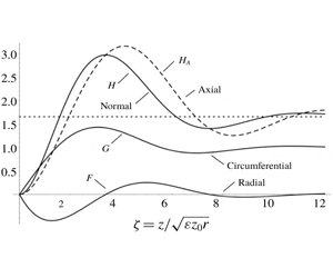
Figure 1. Graphs of the velocity components for turbulent Bödewadt flow using model A. The dotted line is the asymptotic value of the axial velocity component.
The velocity components  $F$,
$F$,  $G$,
$G$,  $H$ and
 $$\begin{eqnarray}H_{A}=H+{\textstyle \frac{1}{2}}\unicode[STIX]{x1D701}F=\sqrt{\unicode[STIX]{x1D70C}}H^{\star }\end{eqnarray}$$
 are graphed versus  $\unicode[STIX]{x1D701}$ in figure 1, with
  $H_{A}$ shown as a dashed curve. The origin of relation (5.3) and its association with the continuity equation (3.7) is explained in appendix A. For comparison, graphs of the solution for the case of laminar flow (i.e. the solution to the Bödewadt problem; see appendix C) are presented in figure 2. Note that the independent variables are different for these two figures. The turbulent solution has larger axial velocity component and larger flow oscillation. Putting numbers to these and other features,
(i) the radial speed reaches a minimum of
$F_{min}=-0.561$ at $\unicode[STIX]{x1D701}_{F}=1.263$;(ii) the circumferential speed reaches a maximum of
$G_{max}=1.435$ at $\unicode[STIX]{x1D701}_{G}=3.084$;(iii) the asymptotic value of the axial speed is
$H_{\infty }=1.659$;(iv) the normal speed reaches a maximum value of
$H_{max}=2.975$ (and $F$ has a zero) at $\unicode[STIX]{x1D701}_{max}=3.390$;(v) the normal speed reaches an internal minimum value of
$H_{min}=1.408$ (and $F$ has a zero) at $\unicode[STIX]{x1D701}_{min}=7.479$; and(vi) the gradient of
$\boldsymbol{V}$ at $\unicode[STIX]{x1D701}=0$ is $0.759{-}0.999\boldsymbol{i}$.


For comparison, the corresponding values for laminar Bödewadt flow are given in appendix C.

Figure 2. Graphs of the velocity components for laminar Bödewadt flow; after figure 11.2 of Schlichting (Reference Schlichting1968).  $\unicode[STIX]{x1D6FA}$ is the rotation rate of the outer fluid. The dotted line is the asymptotic value of the axial velocity component.
The magnitudes of the flow oscillations are illustrated in figure 3, which contains hodographs of the horizontal velocities using model A and laminar Bödewadt flow; compare with figure 11.3 of Schlichting (Reference Schlichting1968). The horizontal velocity is zero at the boundary  $\unicode[STIX]{x1D701}=0$ and varies in a counter-clockwise sense as
  $\unicode[STIX]{x1D701}$ increases, approaching
  $F=0$ and
  $G=1$ as
  $\unicode[STIX]{x1D701}\rightarrow \infty$.

Figure 3. Hodographs of the horizontal velocity using model A and for laminar Bödewadt flow. The dots on the curves denote unit values of  $\unicode[STIX]{x1D701}$:
  $0,1,2,\ldots$.
5.1 Comparison of model A and the laminar Bödewadt model
Model A is similar to the laminar Bödewadt model, in that the diffusivity is independent of axial distance in both models. In fact the momentum equations for these two models are mathematically identical; compare (5.2) with (C 8). However, the models are not physically identical, because the continuity equations and meanings of the quantity  $H$ differ. In Bödewadt flow, lines of constant
  $\unicode[STIX]{x1D701}$ are parallel to lines of constant
  $z$ and, as a consequence,
  $H$ is both the axial speed and the speed normal to lines (in the meridional plane) of constant
  $\unicode[STIX]{x1D701}$. With the turbulent non-dimensionalization, lines of constant
  $\unicode[STIX]{x1D701}$ are tilted relative to lines of constant
  $z$ and consequently there is a difference between
  $H$, which is the speed normal to lines of constant
  $\unicode[STIX]{x1D701}$, and
  $H_{A}$, which is the speed normal to lines of constant
  $z$; see (5.3). The difference between
  $H$ and
  $H_{A}$ is visualized in the inset of figure 12. This distinction between the physical meanings shows up in the continuity equations, which is
  $H^{\prime }+(5/2)F=0$ for the turbulent Bödewadt model and
  $H^{\prime }+2F=0$ for the laminar Bödewadt model; compare (5.1) with (C 5). A physical consequence of this difference is that meridional flow is larger for the turbulent model, as illustrated by the hodographs in figure 3.
Another difference between the laminar and turbulent Bödewadt solutions is in the relation between dimensional and dimensionless axial velocity components. In the laminar case, these two are related by a constant factor  $\sqrt{\unicode[STIX]{x1D708}\unicode[STIX]{x1D6FA}}$, while in the turbulent case, they are related by a factor that depends on
  $r$ (see (3.1) and (3.8)); the dimensional turbulent axial velocity varies as
  $1/\sqrt{r}$. This radial dependence, which is implicit in the solution using model A, is made explicit when investigating the structure of the solution using model B.
6 Turbulent Bödewadt flow using model B
Using model B the turbulent Bödewadt problem consists of equations (3.7) and (3.13) and condition (3.14) with the diffusivity function  $\unicode[STIX]{x1D6EC}$ given by (4.4) and with
  $\unicode[STIX]{x1D703}=1$. Since
  $\unicode[STIX]{x1D6EC}$ now is a function of
  $\unicode[STIX]{x1D70C}$, the solution depends on the specified value of
  $\unicode[STIX]{x1D70C}$ and is necessarily more complicated than that using model A. This problem has been solved using the spectral-iterative procedure described in appendix B for select values of
  $\unicode[STIX]{x1D70C}$, with the results summarized in table 1. Each row of the table represents a converged iteration, with the first column giving the value of
  $\unicode[STIX]{x1D70C}$ and the remaining nine columns containing:
(i)
$z_{1}^{\star }$: the axial location of the first zero of the radial speed;(ii)
$z_{2}^{\star }$: the axial location of second zero of the radial speed;(iii)
$G_{max}$: the maximum circumferential speed;(iv)
$z_{G}^{\star }$: the axial location of this maximum;(v)
$F_{min}$: the minimum radial (i.e. maximum radially inward) speed;(vi)
$z_{F}^{\star }$: the axial location of this minimum;(vii)
$H_{\infty }^{\star }$: the axial speed (outflow) far from the boundary;(viii)
$H_{max}^{\star }$: the maximum axial speed within the boundary layer; and(ix)
$\boldsymbol{V}_{0}^{\prime }\equiv G^{\prime }(0)+\boldsymbol{i}F^{\prime }(0)$: the velocity gradient at the boundary.


Numerical entries are believed to be accurate (within rounding errors).
Table 1. Summary of calculations using model B. The dimensionless radial and axial coordinates  $\unicode[STIX]{x1D70C}$ and
  $z^{\star }$ are defined by (3.2) and (3.4), respectively, and
  $H^{\star }$ is defined by (3.8). For comparison, the last row contains the results using model A, with the entries of the eighth and ninth columns of this last row being
  $H_{\infty }$ and
  $H_{max}$. The underlying calculations have
  $E_{e}<0.01$; see (B 67).

6.1 Visualization of results
When visualizing results obtained using model B the appropriate scaling of the radial and axial coordinates is  $\unicode[STIX]{x1D70C}$ and
  $z^{\star }$ defined by (3.2) and (3.4), respectively. Also, using (3.1), (3.3) and (3.8) the velocity components and their gradients may be expressed as
 $$\begin{eqnarray}\displaystyle \left.\begin{array}{@{}c@{}}\displaystyle \frac{u}{v_{\infty }}=F,\quad \frac{v}{v_{\infty }}=G,\quad \frac{w}{\unicode[STIX]{x1D716}v_{\infty }}=H^{\star },\\ \displaystyle \frac{z_{0}}{v_{\infty }}\frac{\unicode[STIX]{x2202}u}{\unicode[STIX]{x2202}z}=\frac{F^{\prime }}{\sqrt{\unicode[STIX]{x1D70C}}}\quad \text{and}\quad \frac{z_{0}}{v_{\infty }}\frac{\unicode[STIX]{x2202}v}{\unicode[STIX]{x2202}z}=\frac{G^{\prime }}{\sqrt{\unicode[STIX]{x1D70C}}}.\end{array}\right\} & & \displaystyle\end{eqnarray}$$
With this in mind,
(i) values of
$z_{1}^{\star }$, $z_{2}^{\star }$, $z_{G}^{\star }$ and $z_{F}^{\star }$ are graphed versus $\unicode[STIX]{x1D70C}$ in figure 4;(ii) values of
$H_{\infty }^{\star }$ and $H_{max}^{\star }$ are graphed versus $\unicode[STIX]{x1D70C}$ in figure 5;(iii) values of
$F_{min}$ and $G_{max}$ are graphed versus $\unicode[STIX]{x1D70C}$ in figure 6; and(iv) values of
$F^{\prime }/\sqrt{\unicode[STIX]{x1D70C}}$ and $G^{\prime }/\sqrt{\unicode[STIX]{x1D70C}}$ evaluated at $\unicode[STIX]{x1D701}=0$ are graphed versus $\unicode[STIX]{x1D70C}$ in figure 7.


Each of these figures consists of two panels, with graphs in the right-hand panels extending from  $\unicode[STIX]{x1D70C}=0$ to 100 and those the left-hand panels extending from
  $\unicode[STIX]{x1D70C}=0$ to 1.5, in order to show more clearly the structure close to the axis of rotation.

Figure 4. Graphs of the dimensionless axial locations of the first ( $z_{1}^{\star }$) and second (
 $z_{2}^{\star }$) zeros of the radial component of velocity, the maximum (
 $z_{G}^{\star }$) of the circumferential component of velocity and the minimum (
 $z_{F}^{\star }$) of the radial component of velocity using model B: for
  $0<\unicode[STIX]{x1D70C}<100$ in (b) and for
  $0<\unicode[STIX]{x1D70C}\lesssim 1.5$ in (a). The solid curves delimit the domains of radial flow, with the double arrows denoting the direction of flow in the meridional plane. The radial inflow within
  $0<z^{\star }<z_{1}^{\star }$ is the primary jet and the radial outflow within
  $z_{1}^{\star }<z^{\star }<z_{2}^{\star }$ is the secondary jet.

Figure 5. Graphs of the asymptotic ( $H_{\infty }^{\star }$) and maximum (
 $H_{max}^{\star }$) values of the axial velocity component: for
  $0<\unicode[STIX]{x1D70C}<100$ in (b) and for
  $0<\unicode[STIX]{x1D70C}\lesssim 1.5$ in (a).

Figure 6. Graphs of the maximum circumferential ( $G_{max}$) and minimum radial (
 $F_{min}$) velocity components: for
  $0<\unicode[STIX]{x1D70C}<100$ in (b) and for
  $0<\unicode[STIX]{x1D70C}\lesssim 1.5$ in (a).
6.2 Boundary-layer shape
The shape of the boundary layer is illustrated in figure 4, which contains graphs of the dimensionless axial locations  $z_{1}^{\star }$,
  $z_{2}^{\star }$,
  $z_{G}^{\star }$ and
  $z_{F}^{\star }$ versus
  $\unicode[STIX]{x1D70C}$. It is seen that overall the boundary-layer thickness varies roughly linearly with radius, tending to zero at the axis of rotation. There is a departure from linearity for
  $\unicode[STIX]{x1D70C}<1$, with the layer thickness tending toward (but not achieving) the parabolic shape of model A. The variation with
  $\unicode[STIX]{x1D70C}$ of the axial locations seen in this figure may be parameterized by
 $$\begin{eqnarray}z_{y}^{\star }=a_{y}\sqrt{\unicode[STIX]{x1D70C}}+b_{y}\unicode[STIX]{x1D70C}\end{eqnarray}$$
 for  $y=1$, 2,
  $G$ and
  $F$, with
  $a_{1}=2.018$,
  $b_{1}=2.171$,
  $a_{2}=4.391$,
  $b_{2}=9.256$,
  $a_{G}=2.009$,
  $b_{G}=1.128$,
  $a_{F}=0.875$ and
  $b_{F}=0.034$.
The two solid curves in figure 4 visualize the axial locations of the first and second interior zeros of  $F$. Within
  $0<z^{\star }<z_{1}^{\star }$ the flow is radially inward; this is the primary jet; the outward-flowing secondary jet occurs within
  $z_{1}^{\star }<z^{\star }<z_{2}^{\star }$. That is, the lower solid curve marks the top of the primary jet, while the secondary jet lies between these two solid curves, as depicted by the double arrows in the right-hand panel of this figure.
6.3 Velocity magnitudes
The asymptotic ( $H_{\infty }^{\star }$) and maximum (
 $H_{max}^{\star }$) values of the axial velocity component are graphed versus
  $\unicode[STIX]{x1D70C}$ in figure 5. The variation of these velocity components is governed primarily by the factor
  $\sqrt{\unicode[STIX]{x1D70C}}$ appearing in the definition of
  $H^{\star }$ (see (3.8)), with the speeds becoming arbitrarily large as
  $\unicode[STIX]{x1D70C}\rightarrow 0$. For large
  $\unicode[STIX]{x1D70C}$,
  $H_{\infty }^{\star }$ is moderately smaller than
  $H_{max}^{\star }$, indicating that oscillations in the meridional flow are weak. For small
  $\unicode[STIX]{x1D70C}$,
  $H_{max}^{\star }$ is considerably larger than
  $H_{\infty }^{\star }$, indicative of stronger oscillations.
The extreme values of  $F$ and
  $G$ versus
  $\unicode[STIX]{x1D70C}$ are graphed in figure 6. They show little variation, with extremes having greatest magnitude for small
  $\unicode[STIX]{x1D70C}$.
6.4 Gradients at the boundary
The circumferential and radial shear stresses at the boundary are proportional to the gradients of the respective horizontal velocity components; see (6.1). The variation of these gradients with  $\unicode[STIX]{x1D70C}$ is shown in figure 7. As with the axial velocity, the magnitude of the gradients is dominated by the factor
  $\sqrt{\unicode[STIX]{x1D70C}}$, becoming large as
  $\unicode[STIX]{x1D70C}$ decreases.

Figure 7. Graphs of the circumferential (positive values) and radial (negative values) boundary gradients: for  $0<\unicode[STIX]{x1D70C}<100$ in (b) and for
  $0<\unicode[STIX]{x1D70C}\lesssim 1.5$ in (a).
6.5 Flow structure
The structure of the flow is illustrated in figures 8–10 by graphs of the radial ( $F=u/v_{\infty }$), circumferential (
 $G=v/v_{\infty }$) and axial (
 $H^{\star }=\unicode[STIX]{x1D716}w/v_{\infty }$) components of velocity versus
  $z^{\star }$ for select values of
  $\unicode[STIX]{x1D70C}$: 0.1, 1.0, 10.0 and 100.0. The differences of vertical scale at these locations reflect the roughly linear shape of the boundary layer. For large
  $\unicode[STIX]{x1D70C}$, the boundary layer extends far above the top of the rough layer (at
  $z^{\star }=1$), while for
  $\unicode[STIX]{x1D70C}$ small, the boundary layer is comparable in height to the rough layer.

Figure 8. Graphs of the dimensionless radial velocity,  $F$, versus
  $z^{\star }$ at four radial locations as indicated. The vertical dotted lines denote values of
  $F$ in one-tenth intervals. Note the changes in vertical scale.

Figure 9. Graphs of the dimensionless circumferential velocity,  $G$, versus
  $z^{\star }$ at four radial locations as indicated. The vertical dotted lines denote the asymptotic value
  $G=1.0$. Note the changes in vertical scale.

Figure 10. Graphs of the dimensionless axial velocity,  $H^{\star }$, versus
  $z^{\star }$ at four radial locations as indicated. The vertical dashed lines denote the asymptotic values of
  $H^{\star }$. The vertical dotted lines denote values of
  $H^{\star }$ in unit intervals. Note the changes in vertical scale.
All velocity components oscillate as  $z$ increases, with
  $F$ changing sign, while
  $G$ and
  $H^{\star }$ remain positive. The strength of the oscillations increases as
  $\unicode[STIX]{x1D70C}$ decreases. The profiles of
  $F$ and
  $G$ show that for large
  $\unicode[STIX]{x1D70C}$, the boundary layer has a double-layer structure; the radial velocity has a maximum and
  $G$ surpasses unity at a modest value of
  $z^{\star }$, then
  $F$ relaxes to zero and the overshoot of
  $G$ diminishes over a large range of
  $z^{\star }$. For
  $z^{\star }$ of unit order, these large-
 $\unicode[STIX]{x1D70C}$ profiles have similar structure to the well-known logarithmic profiles for turbulent flow near a plane boundary (e.g. see §§ XIX.d and XX.c of Schlichting (Reference Schlichting1968)).
Hodographs of the horizontal velocity components graphed in figures 1, 2, 8 and 9 are presented in figure 11. Note that the strength of the meridional flow, illustrated by radial variation of the hodographs (the vertical in figure 11), is enhanced by boundary roughness and increases with decreasing  $\unicode[STIX]{x1D70C}$.

Figure 11. Hodographs at four radial locations  $\unicode[STIX]{x1D70C}=0.1$, 1.0, 10.0 and 100.0 (shown as dashed curves), together with those using model A and the laminar Bödewadt flow, from figure 3 (shown as solid curves). The dots on the curves denote unit values of
  $\unicode[STIX]{x1D701}$:
  $0,1,2,\ldots$.
7 Discussion of results
When comparing the turbulent Bödewadt-boundary-layer solution in § 6 to the laminar solution found in appendix C, one distinctive feature that stands out is the nearly linear radial variation of boundary-layer thickness in the turbulent model, as shown in figure 4. It is of interest to note that this feature is also seen in models of the boundary layers beneath vortices, both models that explicitly employ a conical transformation (Long Reference Long1958) and those that do not: e.g. see figures 1(a) and 2(a) of Kepert (Reference Kepert2010a), figure 1 of Kepert (Reference Kepert2010b), figures 1(a), 3(a–c), 5(a), 7(a), 11(a,b) and 12(a,b) of Nolan et al. (Reference Nolan, Dahl, Bryan and Rotunno2017) and figure 7 of Part 2. Evidently this structure is a robust feature of realistic models of turbulent boundary layers beneath rotating flows. It follows that models that assume the boundary layer has uniform thickness are incapable of accurately depicting boundary-layer shape.
As previously noted, one feature that is common to both the laminar and turbulent models is the axial oscillations of the velocity components; these oscillations are seen in both analytic solutions (e.g. see figures 4.1, 6.1, 6.2, 6.3 and 6.4 of Kuo (Reference Kuo1971)) and numerical simulations (e.g. see the panels corresponding to  $\unicode[STIX]{x1D714}=0.080$ in figure 10 of Rotunno (Reference Rotunno2013) and figures 3, 5 and 7 of Nolan (Reference Nolan2013)). As noted in § 1.1, these oscillations are induced within the boundary layer by the inertial stability of the axisymmetric rotating flow above; the fluid is capable of sustaining inertial waves. Oscillations of the radial velocity component are manifest as a sequence of jets having strength that diminishes with height. The primary jet, closest to the ground, is strongest and flow is radially inward. The secondary jet immediately above, having radially outward flow, is an essential part of the boundary-layer structure. This jet is apparent in figures 1(a) and 2(a) of Kepert (Reference Kepert2010a). It is shown in Part 2 that these oscillations play an important role in the behaviour of the boundary layer in the vicinity of the eye of a vortex.
The axial structure of the velocity components seen in figures 8, 9 and 10 shows that considerable flow occurs within the rough layer when  $\unicode[STIX]{x1D70C}$ is small. If the boundary layer is much thicker than the rough layer, with little flow occurring within
  $z<z_{0}$, then models using the slip condition can give accurate results. But if the boundary layer is comparable in thickness to the rough layer with significant flow occurring within
  $z<z_{0}$, models using the slip condition may give erroneous results.
7.1 Axial and supergradient flow
There has been some discussion in the literature whether it is correct to specify the circumferential speed at the top of the boundary layer in regions where the axial flow is exiting the layer (e.g. see Smith & Montgomery (Reference Smith and Montgomery2010) and references therein). Smith & Vogl (Reference Smith and Vogl2008) note that ‘It is probably incorrect to prescribe the tangential wind speed just above the boundary layer in the inner region, where the flow exits the boundary layer’. In a similar vein, Smith & Montgomery (Reference Smith and Montgomery2014) argue that prescription of the tangential wind at the top of the boundary layer where the flow is upwards ‘makes the physical problem ill-posed as the boundary layer itself should be allowed to determine the tangential momentum that it expels into the bulk vortex aloft’. These conjectures are based on a misunderstanding of the mathematical nature of boundary-layer flows. A viscous boundary layer is a dynamical structure that provides a smooth variation between the tangential velocity of fluid near a boundary and the velocity of the boundary itself. It is a general feature of these boundary layers that dynamical processes within the layer require an axial (perpendicular to the boundary) flow at the outer edge of the layer. That is, this axial flow is a dependent response to the imposition of an independent tangential velocity difference. In the present context,  $v_{\infty }$ is the independently prescribed velocity difference and
  $w_{\infty }$ is the dependent response. This functional relationship holds whether
  $w_{\infty }$ is positive or negative. If the axial velocity were specified, then it is true that the circumferential velocity could not be. But this is not a physically reasonable approach. The boundary layer is forced by the circumferential velocity, with the axial velocity being determined by the internal dynamics of the boundary layer.
The classic laminar Bödewadt flow (see appendix C) and the turbulent boundary-layer flows presented in this article (see § 6) and in Part 2 all have positive axial flow (out of the boundary layer) for all radii; when the outer flow is rigid-body rotation, fluid is expelled from the boundary layer into the overlying fluid. Provided positive axial flow from the layer also occurs in the case of a swirling outer flow, such flow allows the boundary layer to communicate with – and indirectly to influence – this swirling flow. This communication is not very important to a tornado because there is little dynamical distinction between boundary-layer air and that above. However in a tropical cyclone, typically air within the boundary layer is warm and moist relative to the air above and so has the potential to drive convective motions. A mathematical consequence is that  $v_{\infty }$ and
  $w_{\infty }$ are likely to be coupled functions of
  $r$ for a tropical cyclone, but not for a tornado.
Another issue mentioned in the literature is whether, in regions having vertical outflow from the boundary layer, supergradient flow is expelled and acts to enhance the vortical flow outside the layer (Smith & Vogl Reference Smith and Vogl2008; Kepert Reference Kepert2010a). The solutions presented above show that this is not the case. The supergradient flow is confined to the boundary layer and simply a manifestation of inertial oscillations. This suggests that models exhibiting supergradient flow at the top of the boundary layer may not be accurate.
8 Summary
The turbulent boundary-layer problem formulated in § 2 is a model of the mean flow near a rough non-rotating boundary in the case that the outer fluid (far from the boundary) is in steady, axisymmetric circumferential motion:  $v_{\infty }(r)$. A key feature of the formulation is the assumption that the eddy diffusivity is proportional to the velocity difference across the boundary layer; specifically
  $\unicode[STIX]{x1D708}(r,z)=v_{\infty }(r)L(r,z)$. With this assumption, the viscous terms have a mathematical structure very similar to the inertial terms. Consequently, the outer-flow function
  $v_{\infty }(r)$ plays a more passive role in determining turbulent boundary-layer structure than it would if the flow were laminar.
The effect of outer-flow swirl is quantified by the dimensionless vorticity  $\unicode[STIX]{x1D703}$, defined by (3.9). The problem is cast in non-dimensional form using non-orthogonal coordinates
  $\unicode[STIX]{x1D70C}$ and
  $\unicode[STIX]{x1D701}$ that minimize the influence of the radial-derivative terms in the governing equations. In fact, if
  $\unicode[STIX]{x1D703}$ and
  $L$ are constant (as in model A), the radial-derivative terms are zero and the non-dimensionalization is in fact a similarity transformation. The formulation is further simplified by combining the two components of the momentum equation into a single complex equation. The formulation contains an algebraic singularity, with
  $z\sim \sqrt{\unicode[STIX]{x1D716}z_{0}r}$ and
  $w\sim v_{\infty }\sqrt{\unicode[STIX]{x1D716}z_{0}/r}$. This scaling implies that both the velocity gradient at the boundary and axial outflow from the layer tend to infinity as
  $r$ tends to zero.
The problem consisting of (3.7) and (3.13) (with  $\unicode[STIX]{x1D703}=1$) and boundary conditions (3.14) has been solved, using the spectral-iterative procedure described in appendix B, in the case that the outer flow is in rigid-body motion for two models of the axial variation of the eddy diffusivity. In model A, the diffusivity function
  $L$ is independent of axial distance, while in model B,
  $L$ varies linearly outside a rough layer of thickness
  $z_{0}$ and is constant within that layer. The effect of the rough layer is encapsulated in the dimensionless parameter
  $\unicode[STIX]{x1D70C}=\unicode[STIX]{x1D716}r/z_{0}$, where
  $\unicode[STIX]{x1D716}$ is a small parameter roughly equal to the inverse of the local Reynolds number (see (4.5)). Mathematically model A is the limiting case of model B as
  $\unicode[STIX]{x1D70C}\rightarrow 0$, but the physical interpretation of the results using the two models differ. That is, the results for model A are valid for all radial locations, while the results for model B in the limit
  $\unicode[STIX]{x1D70C}\rightarrow 0$ are valid only at the axis of rotation.
Using model A the boundary-layer shape is strictly parabolic, varying as  $z\sim \sqrt{r}$, for all
  $r$ as dictated by the definition of
  $\unicode[STIX]{x1D701}$; see (3.3). Using model B, the boundary-layer shape is close to linear (
 $z\sim r$) for
  $\unicode[STIX]{x1D70C}>1$, but trending toward parabolic as
  $\unicode[STIX]{x1D70C}\rightarrow 0$. Using model A, the velocity components
  $u$ and
  $v$ are subject to the algebraic singularity through the dependence of
  $\unicode[STIX]{x1D701}$ on
  $r$ but are otherwise independent of
  $r$, while
  $w$ and the velocity gradients at the boundary vary as
  $1/\sqrt{r}$. Using model B,
  $u$,
$u$,  $v$ and
  $\sqrt{r}w$ have modest explicit variation with
  $r$.
$r$.
The boundary-layer solutions using either model and for all parameter values have similar axial structure. The horizontal velocity components decay to zero as exponentially damped oscillations while the axial component decays to a positive constant in a similar fashion. The radial flow consists of a sequence of jets having alternating orientation and successively weaker amplitudes. The primary jet is a strong radial inflow near the ground, as indicated by the radially inward double arrow in figure 4(b), the secondary jet is a weaker radial outflow above, as indicated by the radially outward double arrow in that figure, and so on. Smith, Montgomery & Vogl (Reference Smith, Montgomery and Vogl2008) has found that a secondary jet – flowing radially outward – is an essential feature of a realistic model of meridional flow associated with a boundary layer beneath a vortex. For model A the meridional flow is significantly stronger than that in laminar Bödewadt flow and the axial oscillation of the velocity components are significantly larger. Figures 8–10 show that using model B, the oscillations are weak for large  $\unicode[STIX]{x1D70C}$ and increasing in strength as
  $\unicode[STIX]{x1D70C}$ decreases.
For  $r\gg z_{0}/\unicode[STIX]{x1D716}$ the boundary layer takes on a double-layer structure, with gradients
  $F^{\prime }$ and
  $G^{\prime }$ remaining of unit order close to the bounding plane and the axial locations of zeros of the radial velocity component continually increasing with increasing
  $r$. This suggests that the problem may be amenable to an asymptotic analysis in the limit
  $\unicode[STIX]{x1D716}r/z_{0}\rightarrow \infty$, but this is beyond the scope of this study.
As noted previously, the results described in the § 6 depend quantitatively on the assumed form for the diffusivity function, but the qualitative results summarized in this section are believed to be valid for a wide range of diffusivity models. Also, Kepert (Reference Kepert2010a) finds that the quantitative results of boundary-layer models are fairly insensitive to the specific turbulence model.
One factor motivating this study is a desire to obtain a better understanding of the structure of atmospheric vortices. The present study is a first step, in which the formulation is developed and applied in a simple setting. An obvious drawback of the results presented in §§ 5 and 6 is the assumption of rigid-body flow in the far field. This deficiency will be addressed in Part 2.
Acknowledgements
D. Hoult, P. Roberts and an anonymous referee are thanked for helpful comments and suggestions on the draft manuscript.
Declaration of interests
The authors report no conflict of interest.
Appendix A. Meridional flux balance
This appendix illustrates the form of the vertical velocity in the non-dimensionalization presented in § 3, beginning with the control volume illustrated in figure 12. The flux balance illustrated by this figure is
 $$\begin{eqnarray}Q_{1}=Q_{2}+Q_{3},\end{eqnarray}$$
 where the  $Q$ values are volume fluxes per radian, with
 $$\begin{eqnarray}\displaystyle & \displaystyle Q_{1}=\int _{0}^{\sqrt{\unicode[STIX]{x1D716}z_{0}r}\unicode[STIX]{x1D701}}u(r,z)r\,\text{d}z, & \displaystyle\end{eqnarray}$$
 $$\begin{eqnarray}\displaystyle & \displaystyle Q_{2}=\int _{0}^{\sqrt{\unicode[STIX]{x1D716}z_{0}(r+\unicode[STIX]{x0394}r)}\unicode[STIX]{x1D701}}u(r+\unicode[STIX]{x0394}r,z)(r+\unicode[STIX]{x0394}r)\,\text{d}z & \displaystyle\end{eqnarray}$$
and
 $$\begin{eqnarray}\displaystyle Q_{3} & = & \displaystyle \int _{r}^{(r+\unicode[STIX]{x0394}r)}\boldsymbol{n}\boldsymbol{\cdot }\boldsymbol{v}(\breve{r},\sqrt{\unicode[STIX]{x1D716}z_{0}\breve{r}}\unicode[STIX]{x1D701})\breve{r}\,\text{d}\breve{r}\nonumber\\ \displaystyle & = & \displaystyle \int _{r}^{(r+\unicode[STIX]{x0394}r)}\left(-\frac{1}{2}\sqrt{\frac{\unicode[STIX]{x1D716}z_{0}}{\breve{r}}}\unicode[STIX]{x1D701}u(\breve{r},\sqrt{\unicode[STIX]{x1D716}z_{0}\breve{r}}\unicode[STIX]{x1D701})+w(\breve{r},\sqrt{\unicode[STIX]{x1D716}z_{0}\breve{r}}\unicode[STIX]{x1D701})\right)\breve{r}\,\text{d}\breve{r};\end{eqnarray}$$
the vector
 $$\begin{eqnarray}\boldsymbol{n}=-\frac{1}{2}\sqrt{\frac{\unicode[STIX]{x1D716}z_{0}}{\breve{r}}}\unicode[STIX]{x1D701}\mathbf{1}_{r}+\mathbf{1}_{z}\end{eqnarray}$$
 is normal to the parabola  $\unicode[STIX]{x1D701}=z/\sqrt{\unicode[STIX]{x1D716}z_{0}r}$ = constant and has magnitude equal to the local arc length.

Figure 12. A control volume in the meridional ( $r,z$) plane. The dashed curve is a parabola, on which
  $\unicode[STIX]{x1D701}$ is constant. The inset illustrates the balance quantified by (5.3).
Introducing the non-dimensionalization (3.1) and using (5.3), these flux integrals become
 $$\begin{eqnarray}Q_{1}=rv_{\infty }(r)\sqrt{\unicode[STIX]{x1D716}z_{0}r}\int _{0}^{\unicode[STIX]{x1D701}}F(\breve{\unicode[STIX]{x1D701}},r)\,\text{d}\breve{\unicode[STIX]{x1D701}},\end{eqnarray}$$
 $$\begin{eqnarray}\displaystyle Q_{2} & = & \displaystyle (r+\unicode[STIX]{x0394}r)v_{\infty }(r+\unicode[STIX]{x0394}r)\sqrt{\unicode[STIX]{x1D716}z_{0}(r+\unicode[STIX]{x0394}r)}\int _{0}^{\unicode[STIX]{x1D701}}F(\breve{\unicode[STIX]{x1D701}},r+\unicode[STIX]{x0394}r)\,\text{d}\breve{\unicode[STIX]{x1D701}}\nonumber\\ \displaystyle & {\approx} & \displaystyle Q_{1}+\unicode[STIX]{x0394}r\frac{\text{d}Q_{1}}{\text{d}r}\end{eqnarray}$$
and
 $$\begin{eqnarray}\displaystyle Q_{3} & = & \displaystyle \int _{r}^{(r+\unicode[STIX]{x0394}r)}\left(-{\textstyle \frac{1}{2}}\unicode[STIX]{x1D701}F(\unicode[STIX]{x1D701},\breve{r})+H^{\star }(\unicode[STIX]{x1D701},\breve{r})\right)v_{\infty }(\breve{r})\sqrt{\unicode[STIX]{x1D716}z_{0}\breve{r}}\,\text{d}\breve{r}\nonumber\\ \displaystyle & {\approx} & \displaystyle \unicode[STIX]{x0394}r\left(-{\textstyle \frac{1}{2}}\unicode[STIX]{x1D701}F(\unicode[STIX]{x1D701},r)+H^{\star }(\unicode[STIX]{x1D701},r)\right)v_{\infty }(r)\sqrt{\unicode[STIX]{x1D716}z_{0}r}.\end{eqnarray}$$
 Cancelling out the common factors  $\sqrt{\unicode[STIX]{x1D716}z_{0}}$ and
  $\unicode[STIX]{x0394}r$ and re-arranging, the flux balance is
 $$\begin{eqnarray}\frac{\text{d}}{\text{d}r}\left(r^{3/2}v_{\infty }(r)\int _{0}^{\unicode[STIX]{x1D701}}F(\breve{\unicode[STIX]{x1D701}},r)\,\text{d}\breve{\unicode[STIX]{x1D701}}\right)=\left(\frac{1}{2}\unicode[STIX]{x1D701}F(\unicode[STIX]{x1D701},r)-H^{\star }(\unicode[STIX]{x1D701},r)\right)v_{\infty }(r)\sqrt{r}.\end{eqnarray}$$
 Noting that  $\text{d}v_{\infty }/\text{d}r=(2\unicode[STIX]{x1D703}-1)v_{\infty }/r$ (see (3.9)), balance (A 9) becomes
 $$\begin{eqnarray}\left(2\unicode[STIX]{x1D703}+{\textstyle \frac{1}{2}}\right)\int _{0}^{\unicode[STIX]{x1D701}}F(\breve{\unicode[STIX]{x1D701}},r)\,\text{d}\breve{\unicode[STIX]{x1D701}}+r\int _{0}^{\unicode[STIX]{x1D701}}F_{r}(\breve{\unicode[STIX]{x1D701}},r)\,\text{d}\breve{\unicode[STIX]{x1D701}}={\textstyle \frac{1}{2}}\unicode[STIX]{x1D701}F(\unicode[STIX]{x1D701},r)-H^{\star }(\unicode[STIX]{x1D701},r).\end{eqnarray}$$
 This balance is valid for arbitrary  $\unicode[STIX]{x1D701}$; it follows that
 $$\begin{eqnarray}2\unicode[STIX]{x1D703}F+rF_{r}={\textstyle \frac{1}{2}}\unicode[STIX]{x1D701}F_{\unicode[STIX]{x1D701}}-H_{\unicode[STIX]{x1D701}}^{\star }.\end{eqnarray}$$
This form of the continuity equation is readily converted into (3.7) using (3.2) and (5.3).
Appendix B. Spectral-iterative solution procedure
This appendix describes a procedure for finding the solution to the turbulent boundary-layer problem formulated in § 3, consisting of (3.7) and (3.13) and conditions (3.14). The solution procedure consists of five steps:
(i) transform the semi-infinite domain
$0<\unicode[STIX]{x1D701}<\infty$ to the finite domain $0<\unicode[STIX]{x1D709}<1$ (see § B.1);(ii) restructure the momentum equation (see § B.2);
(iii) representation of the velocity components (see § B.3);
(iv) satisfaction of the governing equation at a set of collocation points (see § B.4); and
(v) an iterative approach to the solution (see § B.5).


The resulting solution is approximate because the series is truncated at a finite number of terms and the iteration is performed a finite number of times. However, the solution can be obtained to any desired accuracy by increasing these two adjustable integers, provided of course that the iteration is convergent.
B.1 Step (i): transformed problem
The first step in the solution procedure is to map the infinite interval  $0<\unicode[STIX]{x1D701}<\infty$ onto the finite interval
  $0<\unicode[STIX]{x1D709}<1$ keeping
  $\unicode[STIX]{x1D70C}$ fixed. This is accomplished by writing
 $$\begin{eqnarray}\unicode[STIX]{x1D701}=\unicode[STIX]{x1D6FC}\unicode[STIX]{x1D70E}(\unicode[STIX]{x1D709}),\end{eqnarray}$$
 where  $\unicode[STIX]{x1D6FC}$ is a specified positive constant and the function
  $\unicode[STIX]{x1D70E}(\unicode[STIX]{x1D709})$ satisfies the boundary constraints
 $$\begin{eqnarray}\unicode[STIX]{x1D70E}(0)=0\quad \unicode[STIX]{x1D70E}^{\prime }(0)=1\quad \text{and}\quad \unicode[STIX]{x1D70E}(1)=\infty .\end{eqnarray}$$
 (A prime denotes differentiation with respect to  $\unicode[STIX]{x1D709}$.) Eliminating
  $\unicode[STIX]{x1D701}$ between (B 1) and (3.3), vertical distance is given by
 $$\begin{eqnarray}z^{\star }\equiv \frac{z}{z_{0}}=\sqrt{\unicode[STIX]{x1D70C}}\unicode[STIX]{x1D6FC}\unicode[STIX]{x1D70E}(\unicode[STIX]{x1D709}).\end{eqnarray}$$
 The formulas presented in the following are expressed in terms of a general transform function  $\unicode[STIX]{x1D70E}(\unicode[STIX]{x1D709})$, while the calculations employ the sigmoid function
 $$\begin{eqnarray}\unicode[STIX]{x1D70E}(\unicode[STIX]{x1D709})=\frac{\unicode[STIX]{x1D709}}{(1-\unicode[STIX]{x1D709})^{\unicode[STIX]{x1D70F}}},\end{eqnarray}$$
 where  $\unicode[STIX]{x1D70F}$ is a second specified positive constant. This function satisfies the boundary constraints (B 2). Also note that
  $\unicode[STIX]{x1D70E}^{\prime \prime }(0)=2\unicode[STIX]{x1D70F}$,
  $\unicode[STIX]{x1D70E}^{\prime \prime \prime }(0)=3(1-\unicode[STIX]{x1D70F})\unicode[STIX]{x1D70F}$ and
  $1/\unicode[STIX]{x1D70E}^{\prime }(1)=0$.
The values of  $\unicode[STIX]{x1D6FC}$ and
  $\unicode[STIX]{x1D70F}$ are to be specified prior to an iteration; a converged solution will not depend on the values of
  $\unicode[STIX]{x1D6FC}$ and
  $\unicode[STIX]{x1D70F}$, but the rate of convergence and accuracy of the iteration procedure will. Roughly speaking, the fraction of collocation points allocated to the rough layer is controlled by the parameter
  $\unicode[STIX]{x1D6FC}$, while the parameter
  $\unicode[STIX]{x1D70F}$ controls the distribution of collocation points above the rough layer. When using model A,
  $\unicode[STIX]{x1D6FC}$ may be varied continuously to obtained the best rate of convergence, while with model B
  $\unicode[STIX]{x1D6FC}$ will be discretized to control the location of the top of the rough layer relative to the collocation points; see § B.4.1.
Note that
 $$\begin{eqnarray}\frac{\unicode[STIX]{x2202}}{\unicode[STIX]{x2202}\unicode[STIX]{x1D701}}=\frac{1}{\unicode[STIX]{x1D6FC}\unicode[STIX]{x1D70E}^{\prime }}\frac{\unicode[STIX]{x2202}}{\unicode[STIX]{x2202}\unicode[STIX]{x1D709}}.\end{eqnarray}$$
 Since  $1/\unicode[STIX]{x1D70E}^{\prime }(1)=0$, the transformed continuity equation is non-singular at
  $\unicode[STIX]{x1D709}=1$ provided
  $F$ is assumed to be linearly proportional to
  $1/\unicode[STIX]{x1D70E}^{\prime }$. The coupling between
  $F$ and
  $G$ in the momentum equation then requires
  $G-1$ to be proportional to
  $1/\unicode[STIX]{x1D70E}^{\prime }$ as well. This line of reasoning leads to expressing the dependent variables as
 $$\begin{eqnarray}\boldsymbol{V}(\unicode[STIX]{x1D70C},\unicode[STIX]{x1D701})=1+\frac{\boldsymbol{v}(\unicode[STIX]{x1D70C},\unicode[STIX]{x1D709})}{\unicode[STIX]{x1D70E}^{\prime }(\unicode[STIX]{x1D709})}\quad \text{and}\quad H(\unicode[STIX]{x1D70C},\unicode[STIX]{x1D701})=\unicode[STIX]{x1D6FC}h(\unicode[STIX]{x1D70C},\unicode[STIX]{x1D709})\end{eqnarray}$$
 for both models A and B, with the understanding that the  $\unicode[STIX]{x1D70C}$ dependence is suppressed when using model A. Substituting (B 6) into (3.7) and (3.13), these governing equations may be expressed as
 $$\begin{eqnarray}h_{\unicode[STIX]{x1D709}}+\left(2\unicode[STIX]{x1D703}+{\textstyle \frac{1}{2}}\right)f+\unicode[STIX]{x1D70C}f_{\unicode[STIX]{x1D70C}}=0,\end{eqnarray}$$
and
 $$\begin{eqnarray}{\mathcal{L}}[\boldsymbol{v}]=\boldsymbol{N},\end{eqnarray}$$
where the linear operator
 $$\begin{eqnarray}{\mathcal{L}}[\boldsymbol{\cdot }]=2\boldsymbol{i}[\boldsymbol{\cdot }]+\frac{1}{\unicode[STIX]{x1D6FC}^{2}}\left(\frac{\unicode[STIX]{x1D706}}{\unicode[STIX]{x1D70E}^{\prime }}\left(\frac{[\boldsymbol{\cdot }]}{\unicode[STIX]{x1D70E}^{\prime }}\right)_{\unicode[STIX]{x1D709}}\right)_{\unicode[STIX]{x1D709}}\end{eqnarray}$$
quantifies the Coriolis and viscous terms, the nonlinear term
 $$\begin{eqnarray}\boldsymbol{N}=h\left(\frac{\boldsymbol{v}}{\unicode[STIX]{x1D70E}^{\prime }}\right)_{\unicode[STIX]{x1D709}}+\unicode[STIX]{x1D70C}f\frac{\boldsymbol{v}_{\unicode[STIX]{x1D70C}}}{\unicode[STIX]{x1D70E}^{\prime }}-2(1-\unicode[STIX]{x1D703})f\left(1+\frac{\boldsymbol{v}}{\unicode[STIX]{x1D70E}^{\prime }}\right)-\boldsymbol{i}\frac{\boldsymbol{v}^{2}}{\unicode[STIX]{x1D70E}^{\prime }}\end{eqnarray}$$
quantifies the inertial terms and
 $$\begin{eqnarray}\unicode[STIX]{x1D706}(\unicode[STIX]{x1D70C},\unicode[STIX]{x1D709})=\unicode[STIX]{x1D6EC}(\unicode[STIX]{x1D70C},\unicode[STIX]{x1D6FC}\unicode[STIX]{x1D70E}(\unicode[STIX]{x1D709}))\end{eqnarray}$$
 is the transformed version of the viscosity function. Note that derivatives with respect to  $\unicode[STIX]{x1D709}$ are denoted by a prime if the variable (e.g.
  $\unicode[STIX]{x1D70E}$) is a function only of
  $\unicode[STIX]{x1D709}$ and by a subscript if the variable depends on both
  $\unicode[STIX]{x1D70C}$ and
  $\unicode[STIX]{x1D709}$.
The function  $\unicode[STIX]{x1D706}$ quantifies the axial variation of the diffusivity function. Using model A, with
  $\unicode[STIX]{x1D6EC}=1$ (see (4.2))
 $$\begin{eqnarray}\unicode[STIX]{x1D706}=1.\end{eqnarray}$$
 With  $\unicode[STIX]{x1D6FC}$,
  $\unicode[STIX]{x1D703}$ and
  $\unicode[STIX]{x1D706}$ being constants (independent of
  $\unicode[STIX]{x1D70C}$), the similarity is preserved; the velocity components are functions only of
  $\unicode[STIX]{x1D709}$. However,
  $\unicode[STIX]{x1D70C}$ does appear in the transform (3.3) and in the relation between the axial and normal velocity (3.8).
Using model B, (4.4) transforms to
 $$\begin{eqnarray}\unicode[STIX]{x1D706}=\left\{\begin{array}{@{}ll@{}}1 & \text{if}~0<\unicode[STIX]{x1D709}\leqslant \unicode[STIX]{x1D709}_{0}\\ \unicode[STIX]{x1D6FC}\sqrt{\unicode[STIX]{x1D70C}}\,\unicode[STIX]{x1D70E}(\unicode[STIX]{x1D709}) & \text{if}~\unicode[STIX]{x1D709}_{0}<\unicode[STIX]{x1D709},\end{array}\right.\end{eqnarray}$$
 where  $\unicode[STIX]{x1D709}_{0}$ is the solution of
 $$\begin{eqnarray}\unicode[STIX]{x1D70E}(\unicode[STIX]{x1D709}_{0})=\frac{1}{\unicode[STIX]{x1D6FC}\sqrt{\unicode[STIX]{x1D70C}}}.\end{eqnarray}$$
 Now  $\unicode[STIX]{x1D706}$ depends on
  $\unicode[STIX]{x1D70C}$ and the radial-derivative terms need to be retained in the governing equations. Since the coordinate transform (B 3) presupposes that
  $\unicode[STIX]{x1D6FC}$ is a constant,
  $\unicode[STIX]{x1D709}_{0}$ is a function of
  $\unicode[STIX]{x1D70C}$ with
 $$\begin{eqnarray}\unicode[STIX]{x1D70E}^{\prime }(\unicode[STIX]{x1D709}_{0})\,\text{d}\unicode[STIX]{x1D709}_{0}=-\frac{\text{d}\unicode[STIX]{x1D70C}}{2\unicode[STIX]{x1D6FC}\unicode[STIX]{x1D70C}^{3/2}}.\end{eqnarray}$$
 The governing equations are to be solved on the interval  $0<\unicode[STIX]{x1D709}<1$, subject to the transformed version of conditions (3.14). In light of the fact that
  $1/\unicode[STIX]{x1D70E}^{\prime }(1)=0$, these are
 $$\begin{eqnarray}\displaystyle \text{at}~\unicode[STIX]{x1D709} & = & \displaystyle 0:\quad \boldsymbol{v}+1=h=0;\end{eqnarray}$$
 $$\begin{eqnarray}\displaystyle \text{at}~\unicode[STIX]{x1D709} & = & \displaystyle 1:\quad \Vert \boldsymbol{v}\Vert <\infty .\end{eqnarray}$$
 The momentum equation (B 8) is satisfied at  $\unicode[STIX]{x1D709}=1$ provided
 $$\begin{eqnarray}\text{at}~\unicode[STIX]{x1D709}=1:\quad \boldsymbol{v}=0.\end{eqnarray}$$
In the following, this condition will be applied instead of the more lax (B 17).
Note that
 $$\begin{eqnarray}\frac{w}{\unicode[STIX]{x1D716}v_{\infty }}=H^{\star }=\frac{\unicode[STIX]{x1D6FC}}{\sqrt{\unicode[STIX]{x1D70C}}}\left(h+\frac{\unicode[STIX]{x1D70E}}{2\unicode[STIX]{x1D70E}^{\prime }}f\right)\end{eqnarray}$$
and
 $$\begin{eqnarray}\frac{w_{\infty }}{\unicode[STIX]{x1D716}v_{\infty }}=\frac{\unicode[STIX]{x1D6FC}}{\sqrt{\unicode[STIX]{x1D70C}}}h|_{\unicode[STIX]{x1D709}=1}.\end{eqnarray}$$
Also, at the bounding plane
 $$\begin{eqnarray}\left.\frac{\unicode[STIX]{x2202}\boldsymbol{V}}{\unicode[STIX]{x2202}\unicode[STIX]{x1D701}}\right|_{\unicode[STIX]{x1D701}=0}=\frac{1}{\unicode[STIX]{x1D6FC}}(\unicode[STIX]{x1D70E}^{\prime \prime }(0)+\boldsymbol{v}^{\prime }(0)).\end{eqnarray}$$
B.1.1 Representation of the radial derivative
When using model B the radial derivatives  $\boldsymbol{v}_{\unicode[STIX]{x1D70C}}$ and
  $f_{\unicode[STIX]{x1D70C}}=\text{Im}[\boldsymbol{v}_{\unicode[STIX]{x1D70C}}]$ need to be quantified. (When using model A,
  $\boldsymbol{v}_{\unicode[STIX]{x1D70C}}=0$.) These are quantified by the first-order forward-difference formula
 $$\begin{eqnarray}\boldsymbol{v}_{\unicode[STIX]{x1D70C}}\approx \frac{\boldsymbol{v}^{+}-\boldsymbol{v}}{\unicode[STIX]{x1D70C}\unicode[STIX]{x1D6FF}},\end{eqnarray}$$
 where  $\boldsymbol{v}^{+}=\boldsymbol{v}(\unicode[STIX]{x1D70C}^{+},\unicode[STIX]{x1D709})$ with
 $$\begin{eqnarray}\unicode[STIX]{x1D70C}^{+}=\unicode[STIX]{x1D70C}(1+\unicode[STIX]{x1D6FF})\end{eqnarray}$$
 and  $\unicode[STIX]{x1D6FF}$ is a specified small positive number. (The forward difference is employed rather than the usual backward difference because the stability of iterative solution procedure improves with increasing
  $\unicode[STIX]{x1D70C}$.) This approximation introduces the variable
  $\boldsymbol{v}^{+}$, which satisfies
 $$\begin{eqnarray}{\mathcal{L}}^{+}[\boldsymbol{v}^{+}]=\boldsymbol{N}^{+},\end{eqnarray}$$
where
 $$\begin{eqnarray}\displaystyle & \displaystyle {\mathcal{L}}^{+}[\boldsymbol{\cdot }]=2\boldsymbol{i}[\boldsymbol{\cdot }]+\frac{1}{\unicode[STIX]{x1D6FC}^{2}}\left(\frac{\unicode[STIX]{x1D706}^{+}}{\unicode[STIX]{x1D70E}^{\prime }}\left(\frac{[\boldsymbol{\cdot }]}{\unicode[STIX]{x1D70E}^{\prime }}\right)_{\unicode[STIX]{x1D709}}\right)_{\unicode[STIX]{x1D709}}, & \displaystyle\end{eqnarray}$$
 $$\begin{eqnarray}\displaystyle & \displaystyle \boldsymbol{N}^{+}=h^{+}\left(\frac{\boldsymbol{v}^{+}}{\unicode[STIX]{x1D70E}^{\prime }}\right)_{\unicode[STIX]{x1D709}}+\unicode[STIX]{x1D70C}^{+}f^{+}\frac{\boldsymbol{v}_{\unicode[STIX]{x1D70C}}^{+}}{\unicode[STIX]{x1D70E}^{\prime }}-2(1-\unicode[STIX]{x1D703})f^{+}\left(1+\frac{\boldsymbol{v}^{+}}{\unicode[STIX]{x1D70E}^{\prime }}\right)-\boldsymbol{i}\frac{(\boldsymbol{v}^{+})^{2}}{\unicode[STIX]{x1D70E}^{\prime }}, & \displaystyle\end{eqnarray}$$
 $$\begin{eqnarray}\displaystyle & \displaystyle \unicode[STIX]{x1D706}^{+}=\left\{\begin{array}{@{}ll@{}}1 & \text{if}~0<\unicode[STIX]{x1D709}\leqslant \unicode[STIX]{x1D709}_{0}^{+}\\ \unicode[STIX]{x1D6FC}\sqrt{\unicode[STIX]{x1D70C}^{+}}\,\unicode[STIX]{x1D70E}(\unicode[STIX]{x1D709}) & \text{if}~\unicode[STIX]{x1D709}_{0}^{+}<\unicode[STIX]{x1D709},\end{array}\right. & \displaystyle\end{eqnarray}$$
and
 $$\begin{eqnarray}\unicode[STIX]{x1D709}_{0}^{+}=\unicode[STIX]{x1D709}_{0}-\frac{\unicode[STIX]{x1D6FF}}{2\unicode[STIX]{x1D6FC}\sqrt{\unicode[STIX]{x1D70C}}\unicode[STIX]{x1D70E}^{\prime }(\unicode[STIX]{x1D709}_{0})}\end{eqnarray}$$
 (see (B 15)). The variable  $h^{+}$ satisfies
 $$\begin{eqnarray}h_{\unicode[STIX]{x1D709}}^{+}+\left(2\unicode[STIX]{x1D703}+{\textstyle \frac{1}{2}}\right)f^{+}+\unicode[STIX]{x1D70C}^{+}f_{\unicode[STIX]{x1D70C}}^{+}=0.\end{eqnarray}$$
 The system of equations is closed by approximating the radial derivative at  $\unicode[STIX]{x1D70C}^{+}$ by a backward difference
 $$\begin{eqnarray}\boldsymbol{v}_{\unicode[STIX]{x1D70C}}^{+}\approx \frac{\boldsymbol{v}^{+}-\boldsymbol{v}}{\unicode[STIX]{x1D70C}\unicode[STIX]{x1D6FF}}.\end{eqnarray}$$
The major challenge at hand is to obtain solutions of the nonlinear momentum equations (B 8) and (B 24). Solutions can be found using an iterative procedure provided these equations are suitably restructured, as explained in step (ii).
B.2 Step (ii): restructuring the momentum equation
Momentum equations (B 8) and (B 24) may be recast in forms that are amenable to iterative solution by writing
 $$\begin{eqnarray}\{\boldsymbol{v},\boldsymbol{v}^{+}\}=\{\widetilde{\boldsymbol{v}},\widetilde{\boldsymbol{v}}^{+}\}+\{\widehat{\boldsymbol{v}},\widehat{\boldsymbol{v}}^{+}\},\end{eqnarray}$$
 where  $\widetilde{\boldsymbol{v}}$ and
  $\widetilde{\boldsymbol{v}}^{+}$ are known approximations and
  $\widehat{\boldsymbol{v}}$ and
  $\widehat{\boldsymbol{v}}^{+}$ are unknown improvements. Substituting (B 31) into momentum equations (B 8) and (B 24), these may be expressed as
 $$\begin{eqnarray}\{{\mathcal{L}}[\widehat{\boldsymbol{v}}],{\mathcal{L}}^{+}[\widehat{\boldsymbol{v}}^{+}]\}=\{\widetilde{\boldsymbol{E}},\widetilde{\boldsymbol{E}}^{+}\}+\{\widehat{\boldsymbol{M}},\widehat{\boldsymbol{M}}^{+}\},\end{eqnarray}$$
 where  ${\mathcal{L}}[\boldsymbol{\cdot }]$ and
  ${\mathcal{L}}^{+}[\boldsymbol{\cdot }]$ (defined by (B 9) and (B 25)) are linear operators with known coefficients,
 $$\begin{eqnarray}\{\widetilde{\boldsymbol{E}},\widetilde{\boldsymbol{E}}^{+}\}=\{\widetilde{\boldsymbol{N}},\widetilde{\boldsymbol{N}}^{+}\}-\{{\mathcal{L}}[\widetilde{\boldsymbol{v}}],{\mathcal{L}}^{+}[\widetilde{\boldsymbol{v}}^{+}]\},\end{eqnarray}$$
 $\widetilde{\boldsymbol{N}}$ and
  $\widetilde{\boldsymbol{N}}^{+}$ are given by (B 10) and (B 26) with tildes added to all the velocity components and
  $\widehat{\boldsymbol{M}}$ and
  $\widehat{\boldsymbol{M}}^{+}$ are complicated complex functions containing products of approximations and improvements. The forms of
  $\widehat{\boldsymbol{M}}$ and
  $\widehat{\boldsymbol{M}}^{+}$ are unimportant as these terms will be ignored, with the simplified equations
 $$\begin{eqnarray}\{{\mathcal{L}}[\widehat{\boldsymbol{v}}],{\mathcal{L}}^{+}[\widehat{\boldsymbol{v}}^{+}]\}=\{\widetilde{\boldsymbol{E}},\widetilde{\boldsymbol{E}}^{+}\}\end{eqnarray}$$
 to be solved, rather than (B 32). Equations (B 34) will be solved iteratively for  $\widehat{\boldsymbol{v}}$ and
  $\widehat{\boldsymbol{v}}^{+}$ with the improvement being successively added to the approximation, as explained in § B.4. In a converged solution, the approximations are the desired result, with the improvement
  $\widehat{\boldsymbol{v}}$ and
  $\widehat{\boldsymbol{v}}^{+}$ being negligibly small and with each of the functions
  $\widetilde{\boldsymbol{E}}$,
  $\widetilde{\boldsymbol{E}}^{+}$,
  ${\mathcal{L}}[\widehat{\boldsymbol{v}}]$,
  ${\mathcal{L}}^{+}[\widehat{\boldsymbol{v}}^{+}]$,
  $\widehat{\boldsymbol{M}}$ and
  $\widehat{\boldsymbol{M}}^{+}$ being effectively equal to zero.
Stipulating that the approximations satisfy conditions
 $$\begin{eqnarray}\displaystyle \text{at}~\unicode[STIX]{x1D709} & = & \displaystyle 0:\quad \{\widetilde{\boldsymbol{v}},\widetilde{\boldsymbol{v}}^{+}\}+1=0;\end{eqnarray}$$
 $$\begin{eqnarray}\displaystyle \text{at}~\unicode[STIX]{x1D709} & = & \displaystyle 1:\quad \{\widetilde{\boldsymbol{v}},\widetilde{\boldsymbol{v}}^{+}\}=0,\end{eqnarray}$$
conditions (B 16) and (B 18) require that the improvements satisfy
 $$\begin{eqnarray}\displaystyle \text{at}~\unicode[STIX]{x1D709} & = & \displaystyle 0:\quad \{\widehat{\boldsymbol{v}},\widehat{\boldsymbol{v}}^{+}\}=0;\end{eqnarray}$$
 $$\begin{eqnarray}\displaystyle \text{at}~\unicode[STIX]{x1D709} & = & \displaystyle 1:\quad \{\widehat{\boldsymbol{v}},\widehat{\boldsymbol{v}}^{+}\}=0.\end{eqnarray}$$
 In summary, the problem consists of continuity equations (B 7) and (B 29) and momentum equations (B 34) with  $\unicode[STIX]{x1D706}$ given by (B 12) when using model A,
  $\unicode[STIX]{x1D706}$ and
  $\unicode[STIX]{x1D706}^{+}$ given by (B 13) and (B 27) when using model B and
  $\boldsymbol{v}_{\unicode[STIX]{x1D70C}}$ and
  $\boldsymbol{v}_{\unicode[STIX]{x1D70C}}^{+}$ given by (B 22) and (B 30), respectively. When using model A, the variables with superscript
  $+$ are irrelevant and may be ignored. Harmonic representations of
  $h$ and
  $h^{+}$ appropriate to the continuity equations are given in § B.3.1 and harmonic representations of the improvements
  $\widehat{\boldsymbol{v}}$ and
  $\widehat{\boldsymbol{v}}^{+}$ appropriate to the momentum equations are given in § B.3.2. Representation of the approximations
  $\widetilde{\boldsymbol{v}}$ and
  $\widetilde{\boldsymbol{v}}^{+}$ is necessarily a bit more complicated, as explained in the following subsection.
B.2.1 Elements of the approximations
The approximations  $\widetilde{\boldsymbol{v}}$ and
  $\widetilde{\boldsymbol{v}}^{+}$ are composed of three elements: starting polynomials (denoted by subscript
  $s$), accumulated improvements (denoted by an overbar) and supplemental polynomials (denoted by a breve)
 $$\begin{eqnarray}\{\widetilde{\boldsymbol{v}},\widetilde{\boldsymbol{v}}^{+}\}=\boldsymbol{v}_{s}+\{\overline{\boldsymbol{v}},\overline{\boldsymbol{v}}^{+}\}+\{\breve{\boldsymbol{v}},\breve{\boldsymbol{v}}^{+}\}.\end{eqnarray}$$
 The starting polynomials satisfy the non-homogeneous boundary condition (B 35) and serve as a seed to initiate the iteration. The accumulated improvements are the judicious sum of the improvements found at each iteration; see § B.3.2. The supplemental polynomials ensure satisfaction of the governing equations at the endpoints  $\unicode[STIX]{x1D709}=0$ and 1 and continuity of the governing equations at the top of the rough layer
  $\unicode[STIX]{x1D709}=\unicode[STIX]{x1D709}_{0}$. The starting polynomials are invariant during an iteration, while the accumulated improvements and supplemental polynomials are updated at each step. A converged solution is independent of the specific forms of the starting and supplemental polynomials. Reasonable forms of these polynomials are presented in §§ B.3.3 and B.3.4, respectively.
Boundary conditions (B 35) and (B 36) are satisfied by specifying that
 $$\begin{eqnarray}\displaystyle \text{at}~\unicode[STIX]{x1D709} & = & \displaystyle 0:\quad \boldsymbol{v}_{s}+1=0;\end{eqnarray}$$
 $$\begin{eqnarray}\displaystyle \text{at}~\unicode[STIX]{x1D709} & = & \displaystyle 1:\quad \boldsymbol{v}_{s}=0\end{eqnarray}$$
 so that the variables  $\overline{\boldsymbol{v}}$,
  $\overline{\boldsymbol{v}}^{+}$,
  $\breve{\boldsymbol{v}}$ and
  $\breve{\boldsymbol{v}}^{+}$ satisfy the homogeneous conditions
 $$\begin{eqnarray}\displaystyle \text{at}~\unicode[STIX]{x1D709} & = & \displaystyle 0:\quad \boldsymbol{v}=0;\end{eqnarray}$$
 $$\begin{eqnarray}\displaystyle \text{at}~\unicode[STIX]{x1D709} & = & \displaystyle 1:\quad \boldsymbol{v}=0.\end{eqnarray}$$
B.3 Step (iii): representations
The axial velocity components  $h$ and
  $h^{+}$ are fairly simple and can be represented by Fourier cosine series, as explained in § B.3.1. The complex horizontal velocity components are somewhat more complicated, consisting of improvements represented by Fourier sine series, as explained in § B.3.2, a starting polynomial given in § B.3.3 and a supplemental polynomial given in § B.3.4.
B.3.1 Representation of $h$ and $h^{+}$


The normal velocity components  $h$ and
  $h^{+}$ satisfy equations (B 7) and (B 29) with
  $f=\widetilde{f}$ and
  $f^{+}=\widetilde{f}^{+}$ and boundary conditions
  $h=h^{+}=0$ at
  $\unicode[STIX]{x1D709}=0$. Since
  $\widetilde{f}$ and
  $\widetilde{f}^{+}$ are zero at
  $\unicode[STIX]{x1D709}=0$ and 1,
  $h_{\unicode[STIX]{x1D709}}=h_{\unicode[STIX]{x1D709}}^{+}=0$ at
  $\unicode[STIX]{x1D709}=0$ and 1. Forms satisfying these conditions are
 $$\begin{eqnarray}\{h,h^{+}\}=\mathop{\sum }_{j=1}^{K_{h}}\{h_{k},h_{k}^{+}\}\frac{\cos (k\unicode[STIX]{x03C0}\unicode[STIX]{x1D709})-1}{k\unicode[STIX]{x03C0}},\end{eqnarray}$$
 where  $K_{h}$ is a specified integer. Now (B 7) and (B 29) become
 $$\begin{eqnarray}\mathop{\sum }_{j=1}^{K_{h}}\{h_{k},h_{k}^{+}\}\sin (k\unicode[STIX]{x03C0}\unicode[STIX]{x1D709})=\{C,C^{+}\},\end{eqnarray}$$
where
 $$\begin{eqnarray}\{C,C^{+}\}=\left(2\unicode[STIX]{x1D703}+\frac{1}{2}\right)\{\widetilde{f},\widetilde{f}^{+}\}+\frac{\widetilde{f}^{+}-\widetilde{f}}{\unicode[STIX]{x1D6FF}}.\end{eqnarray}$$
Equations (B 45) are readily solved by collocation and matrix inversion; see § B.4.
B.3.2 Representation of improvements
Homogeneous boundary conditions (B 37), (B 38), (B 42) and (B 43) are automatically satisfied if the improvements (denoted by carets) and accumulated improvements (denoted by overbars) are expressed in terms of a Fourier sine series
 $$\begin{eqnarray}x=\mathop{\sum }_{k=1}^{K}x_{k}\sin (k\unicode[STIX]{x03C0}\unicode[STIX]{x1D709})\end{eqnarray}$$
 for  $x=\widehat{\boldsymbol{v}}$,
  $\overline{\boldsymbol{v}}$,
  $\widehat{\boldsymbol{v}}^{+}$ and
  $\overline{\boldsymbol{v}}^{+}$, where
  $K$ is a specified integer.
Operating on (B 47) with  ${\mathcal{L}}$ and
  ${\mathcal{L}}^{+}$, which are given by (B 9) and (B 25), the differential operations become algebraic
 $$\begin{eqnarray}\{{\mathcal{L}}[x],{\mathcal{L}}^{+}[x^{+}]\}=\mathop{\sum }_{k=1}^{K}\{\boldsymbol{L}_{k}x_{k},\boldsymbol{L}_{k}^{+}x_{k}^{+}\}\end{eqnarray}$$
 for  $x=\widehat{\boldsymbol{v}}$ and
  $\overline{\boldsymbol{v}}$, where
 $$\begin{eqnarray}\{\boldsymbol{L}_{k},\boldsymbol{L}_{k}^{+}\}=2\boldsymbol{i}\sin (k\unicode[STIX]{x03C0}\unicode[STIX]{x1D709})+\frac{1}{\unicode[STIX]{x1D6FC}^{2}}\left(\frac{\{\unicode[STIX]{x1D706},\unicode[STIX]{x1D706}^{+}\}}{\unicode[STIX]{x1D70E}^{\prime }}\left(\frac{\sin (k\unicode[STIX]{x03C0}\unicode[STIX]{x1D709})}{\unicode[STIX]{x1D70E}^{\prime }}\right)_{\unicode[STIX]{x1D709}}\right)_{\unicode[STIX]{x1D709}}\end{eqnarray}$$
are known complex functions. Now (B 34) may be expressed as
 $$\begin{eqnarray}\mathop{\sum }_{k=1}^{K}\{\boldsymbol{L}_{k}\widehat{\boldsymbol{v}}_{k},\boldsymbol{L}_{k}^{+}\widehat{\boldsymbol{v}}_{k}^{+}\}=\{\widetilde{\boldsymbol{E}},\widetilde{\boldsymbol{E}}^{+}\},\end{eqnarray}$$
 where  $\widetilde{\boldsymbol{E}}$ and
  $\widetilde{\boldsymbol{E}}^{+}$ are given by (B 33). These equations are to be solve iteratively for the coefficients
  $\widehat{\boldsymbol{v}}_{k}$ and
  $\widehat{\boldsymbol{v}}_{k}^{+}$, with the terms on the right-hand side updated at each step.
The coefficients  $\overline{\boldsymbol{v}}_{k}$ and
  $\overline{\boldsymbol{v}}_{k}^{+}$ are the weighted sum of the values of
  $\widehat{\boldsymbol{v}}_{k}$ and
  $\widehat{\boldsymbol{v}}_{k}^{+}$ found during previous iterations. Updating needs to be done judiciously, because the improvements overshoot the mark when
  $\unicode[STIX]{x1D70C}$ is small, causing the iteration to diverge. In order to avoid this undesirable result, at each iteration the coefficients will be updated by the replacements
 $$\begin{eqnarray}\overline{\boldsymbol{v}}_{k}+\unicode[STIX]{x1D6FE}\widehat{\boldsymbol{v}}_{k}\rightarrow \overline{\boldsymbol{v}}_{k}\end{eqnarray}$$
 and similarly for  $\overline{\boldsymbol{v}}_{k}^{+}$, where
  $\unicode[STIX]{x1D6FE}$ is an adjustable parameter satisfying
  $0<\unicode[STIX]{x1D6FE}\leqslant 1$.
B.3.3 Representation of starting polynomials
The starting polynomials (denoted by subscript  $s$) satisfy conditions (B 40) and (B 41), thereby providing a seed to initiate the iteration procedure. In addition, they are constructed such that the functions
  $\widetilde{\boldsymbol{E}}$ and
  $\widetilde{\boldsymbol{E}}^{+}$, defined by (B 33), are equal to 0 at
  $\unicode[STIX]{x1D709}=0$.
The starting polynomials are
 $$\begin{eqnarray}\displaystyle f_{s}=\,f_{s}^{+} & = & \displaystyle -\frac{\unicode[STIX]{x1D6FC}^{2}}{3(2+\unicode[STIX]{x1D70E}^{\prime \prime }(0))}(1-2\unicode[STIX]{x1D709})(1-\unicode[STIX]{x1D709})\unicode[STIX]{x1D709}\nonumber\\ \displaystyle & = & \displaystyle -\frac{\unicode[STIX]{x1D6FC}^{2}}{6(1+\unicode[STIX]{x1D70F})}(1-2\unicode[STIX]{x1D709})(1-\unicode[STIX]{x1D709})\unicode[STIX]{x1D709}\end{eqnarray}$$
and
 $$\begin{eqnarray}\displaystyle g_{s}=g_{s}^{+} & = & \displaystyle -\left(1+\frac{3\unicode[STIX]{x1D70E}^{\prime \prime }(0)+3\left(\unicode[STIX]{x1D70E}^{\prime \prime }(0)\right)^{2}-\unicode[STIX]{x1D70E}^{\prime \prime \prime }(0)}{2+3\unicode[STIX]{x1D70E}^{\prime \prime }(0)}\unicode[STIX]{x1D709}\right)(1-\unicode[STIX]{x1D709})\nonumber\\ \displaystyle & = & \displaystyle -\left(1+\frac{3}{2}\unicode[STIX]{x1D70F}\unicode[STIX]{x1D709}\right)(1-\unicode[STIX]{x1D709}),\end{eqnarray}$$
 with  $\boldsymbol{v}_{s}=g_{s}+\boldsymbol{i}f_{s}$ and
  $\boldsymbol{v}_{s}^{+}=g_{s}^{+}+\boldsymbol{i}f_{s}^{+}$.
B.3.4 Representation of supplemental polynomials
The supplemental polynomials (denoted by a breve) serve two related functions; they ensure the approximations to the momentum equation  $\widetilde{\boldsymbol{E}}$ and
  $\widetilde{\boldsymbol{E}}^{+}$ are zero at
  $\unicode[STIX]{x1D709}=0$ and (for model B) are continuous at
  $\unicode[STIX]{x1D709}=\unicode[STIX]{x1D709}_{0}$. The forms satisfying the condition that
  $\widetilde{\boldsymbol{E}}=0$ at
  $\unicode[STIX]{x1D709}=0$ are
 $$\begin{eqnarray}\breve{f}=-2(1-\unicode[STIX]{x1D709})^{3}\unicode[STIX]{x1D709}\overline{f}_{\unicode[STIX]{x1D709}}|_{\unicode[STIX]{x1D709}=0},\end{eqnarray}$$
and

with  Forms satisfying the condition that
  $\widetilde{\boldsymbol{E}}^{+}=0$ at
  $\unicode[STIX]{x1D709}=0$ are obtained by simply adding superscripts
  $+$ to
  $f$ and
  $g$ in these formulas.
Continuity of the approximation  $\widetilde{\boldsymbol{E}}$ at
  $\unicode[STIX]{x1D709}=\unicode[STIX]{x1D709}_{0}$ is achieved by amending the supplemental functions in the interval
  $\unicode[STIX]{x1D709}_{0}<\unicode[STIX]{x1D709}<1$; that is,
 $$\begin{eqnarray}\widetilde{\boldsymbol{v}}\Rightarrow \left\{\begin{array}{@{}ll@{}}\widetilde{\boldsymbol{v}} & \text{if}~0<\unicode[STIX]{x1D709}\leqslant \unicode[STIX]{x1D709}_{0}\\ \widetilde{\boldsymbol{v}}+\grave{\boldsymbol{v}} & \text{if}~\unicode[STIX]{x1D709}_{0}<\unicode[STIX]{x1D709}<1\end{array}\right.\end{eqnarray}$$
with
 $$\begin{eqnarray}\grave{\boldsymbol{v}}=\left.\left(\frac{\unicode[STIX]{x1D70E}^{\prime \prime }}{\unicode[STIX]{x1D70E}}\widetilde{\boldsymbol{v}}-\frac{\unicode[STIX]{x1D70E}^{\prime }}{\unicode[STIX]{x1D70E}}\widetilde{\boldsymbol{v}}_{\unicode[STIX]{x1D709}}\right)\right|_{\unicode[STIX]{x1D709}=\unicode[STIX]{x1D709}_{0}}p_{3}^{\prime },\end{eqnarray}$$
where
 $$\begin{eqnarray}p_{3}=\frac{1}{6}(1-\unicode[STIX]{x1D709})^{2}\left(\frac{\unicode[STIX]{x1D709}-\unicode[STIX]{x1D709}_{0}}{1-\unicode[STIX]{x1D709}_{0}}\right)^{3}.\end{eqnarray}$$
 Similarly, continuity of the approximation  $\widetilde{\boldsymbol{E}}^{+}$ at
  $\unicode[STIX]{x1D709}=\unicode[STIX]{x1D709}_{0}^{+}$ is achieved by replacing
  $\unicode[STIX]{x1D709}_{0}$ with
  $\unicode[STIX]{x1D709}_{0}^{+}$ and
  $\widetilde{\boldsymbol{v}}$ with
  $\widetilde{\boldsymbol{v}}^{+}$ in these formulas.
To sum up, the problem consists of the algebraic equations (B 50) to be solved for  $\widehat{\boldsymbol{v}}_{k}$ and
  $\widehat{\boldsymbol{v}}_{k}^{+}$ and algebraic equations (B 45) to be solved for
  $h$ and
  $h^{+}$ with
(i)
${\mathcal{L}}$ and ${\mathcal{L}}^{+}$ given by (B 9) and (B 25), respectively;(ii)
$\unicode[STIX]{x1D70E}$ given by (B 4);(iii)
$\unicode[STIX]{x1D706}=1$ for model A and $\unicode[STIX]{x1D706}$ and $\unicode[STIX]{x1D706}^{+}$ given by (B 13) and (B 27) for model B;(iv)
$\widetilde{\boldsymbol{E}}$ and $\widetilde{\boldsymbol{E}}^{+}$ given by (B 33);(v)
$\widetilde{\boldsymbol{N}}$ and $\widetilde{\boldsymbol{N}}^{+}$ given by (B 10) and (B 26);(vi)
$\widetilde{\boldsymbol{v}}$ expressed as the sum of $\boldsymbol{v}_{s}$, $\overline{\boldsymbol{v}}$ and $\breve{\boldsymbol{v}}$ and $\widetilde{\boldsymbol{v}}^{+}$ expressed as the sum of $\boldsymbol{v}_{s}$, $\overline{\boldsymbol{v}}^{+}$ and $\breve{\boldsymbol{v}}^{+}$ (see (B 39));(vii)
$\boldsymbol{v}_{s}=g_{s}+\boldsymbol{i}f_{s}$ given by (B 52) and (B 53);(viii)
$\overline{\boldsymbol{v}}$ and $\overline{\boldsymbol{v}}^{+}$ given by (B 47) with $\overline{\boldsymbol{v}}_{k}$ and $\overline{\boldsymbol{v}}_{k}^{+}$ being successively updated according to (B 51);(ix)
and given by (B 54) and (B 55) and $\grave{\boldsymbol{v}}$ and $\grave{\boldsymbol{v}}^{+}$ given by (B 57).


 and
and  given by (

Unlike the starting polynomials that are invariant during the iteration procedure, the supplemental polynomials are updated during each iteration step. This updating procedure involves evaluations of the accumulated improvements  $\overline{\boldsymbol{v}}=\overline{g}+\boldsymbol{i}\overline{f}$ and
  $\overline{\boldsymbol{v}}^{+}=\overline{g}^{+}+\boldsymbol{i}\overline{f}^{+}$ at
  $\unicode[STIX]{x1D709}=\unicode[STIX]{x1D709}_{0}$ and their derivatives at both
  $\unicode[STIX]{x1D709}=0$ and
  $\unicode[STIX]{x1D709}_{0}$.
B.4 Collocation
The essence of the spectral method is to determine the unknown coefficients,  $h_{k}$,
  $h_{k}^{+}$,
  $\widehat{\boldsymbol{v}}_{k}$ and
  $\widehat{\boldsymbol{v}}_{k}^{+}$, by satisfying (B 45) and (B 50) at a set of collocation points, equally spaced on the interval
  $0<\unicode[STIX]{x1D709}<1$
 $$\begin{eqnarray}\unicode[STIX]{x1D709}_{j}=\frac{j}{K+1}\quad \text{for}~j=1\rightarrow K.\end{eqnarray}$$
 The number of points chosen to represent  $h$ and
  $h^{+}$ (denoted by
  $K_{h}$) may differ from the number
  $K$ chosen to represent
  $\widehat{\boldsymbol{v}}$,
  $\widehat{\boldsymbol{v}}^{+}$,
  $\overline{\boldsymbol{v}}$ and
  $\overline{\boldsymbol{v}}^{+}$.
The collocated forms of (B 45) and (B 50) are
 $$\begin{eqnarray}\mathop{\sum }_{k=1}^{K_{h}}S_{kj}\{h_{k},h_{k}^{+}\}=\{C_{j},C_{j}^{+}\}\end{eqnarray}$$
and
 $$\begin{eqnarray}\mathop{\sum }_{k=1}^{K}\{\boldsymbol{L}_{kj}\widehat{\boldsymbol{v}}_{k},\boldsymbol{L}_{kj}^{+}\widehat{\boldsymbol{v}}_{k}^{+}\}=\{\widetilde{\boldsymbol{E}}_{j},\widetilde{\boldsymbol{E}}_{j}^{+}\},\end{eqnarray}$$
where
 $$\begin{eqnarray}S_{kj}=\sin (k\unicode[STIX]{x03C0}\unicode[STIX]{x1D709}_{j})\end{eqnarray}$$
 and a subscript  $j$ means evaluation at
  $\unicode[STIX]{x1D709}=\unicode[STIX]{x1D709}_{j}$ for
  $j$ running from 1 to
  $K_{h}$ or
  $K$. These equations are readily solved by matrix inversion
 $$\begin{eqnarray}\{h_{k},h_{k}^{+}\}=\mathop{\sum }_{j=1}^{K_{h}}[S_{kj}]^{-1}\{C_{j},C_{j}^{+}\}\end{eqnarray}$$
and
 $$\begin{eqnarray}\{\widehat{\boldsymbol{v}}_{k},\widehat{\boldsymbol{v}}_{k}^{+}\}=\mathop{\sum }_{j=1}^{K}\{[\boldsymbol{L}_{kj}]^{-1}\widetilde{\boldsymbol{E}}_{j},[\boldsymbol{L}_{kj}^{+}]^{-1}\widetilde{\boldsymbol{E}}_{j}^{+}\},\end{eqnarray}$$
 where  $[S_{kj}]^{-1}$,
  $[\boldsymbol{L}_{kj}]^{-1}$ and
  $[\boldsymbol{L}_{kj}^{+}]^{-1}$ are the inverse of the transpose of
  $S_{kj}$,
  $\boldsymbol{L}_{kj}$ and
  $\boldsymbol{L}_{kj}^{+}$, respectively. Equation (B 63) can be solved in one step, but (B 64) is solved iteratively until
  $\widetilde{\boldsymbol{E}}_{j}$ and
  $\widetilde{\boldsymbol{E}}_{j}^{+}$ are effectively zero, with (B 63) being updated at each step.
B.4.1 Spacing of collocation points
The diffusivity function for model B, given variously by (4.3), (4.4) and (B 11), is not analytic at the break point  $\unicode[STIX]{x1D709}=\unicode[STIX]{x1D709}_{0}$ and graphs of the real and imaginary parts of the equation error (introduced in § B.6.2) have sharp spikes at this point. These errors are regularized by locating
  $\unicode[STIX]{x1D709}_{0}$ at the midpoint between two adjacent collocation points. This is accomplished by setting
 $$\begin{eqnarray}\unicode[STIX]{x1D709}_{0}=\frac{1+2K_{r}}{2+2K},\end{eqnarray}$$
 where the integer  $K_{r}$ is the number of collocation points within the rough layer, with
  $0\leqslant K_{r}<K$. Previously, the value of
  $\unicode[STIX]{x1D6FC}$ was prescribed, with
  $\unicode[STIX]{x1D709}_{0}$ given in terms of
  $\unicode[STIX]{x1D6FC}$ and
  $\unicode[STIX]{x1D70C}$ by (B 14). Now the integer
  $K_{r}$ is prescribed and
  $\unicode[STIX]{x1D709}_{0}$ is given by (B 65) with (B 14) determining
  $\unicode[STIX]{x1D6FC}$. Constancy of
  $\unicode[STIX]{x1D6FC}$ for the parallel iteration is assured by specifying
  $\unicode[STIX]{x1D709}_{0}^{+}$ using (B 28).
The continuous problem using model B presented in § B.2 is singular in the limit  $\unicode[STIX]{x1D70C}\rightarrow \infty$ (that is, as
  $z_{0}\rightarrow 0$). However, the collocated problem presented earlier in this section is not. Singular behaviour near
  $\unicode[STIX]{x1D709}=0$ has been eliminated by representing the velocity components in terms of Fourier series. This regularization of the collocated problem permits solution in the case that no collocation points fall within the rough layer.
B.5 Iteration
The fifth and last step of the solution procedure is to solve the discretized problem iteratively. The iterative solution procedure is preceded by some preliminary steps, as follows:
(I) choose values of:
(i) the parameters
$\unicode[STIX]{x1D703}$ and (for model B) $\unicode[STIX]{x1D70C}$;(ii) the number of collocation points for the vertical velocity (
$K_{h}$), for the horizontal velocity ($K$) and within the rough layer ($K_{r}$);(iii) the fractional radial distance
$\unicode[STIX]{x1D6FF}$ between the parallel iteration;(iv) the transform exponent
$\unicode[STIX]{x1D70F}$;(v) the stopping criteria
$E_{min}$ and $E_{max}$ (see § B.6.1),(vi) the maximum iteration count
$C_{m}$; and(vii) the additive parameter
$\unicode[STIX]{x1D6FE}$ (see (B 51));
(II) evaluate
$\unicode[STIX]{x1D709}_{0}$ using (B 65), $\unicode[STIX]{x1D6FC}$ using (B 14), $\unicode[STIX]{x1D70C}^{+}$ using (B 23) and $\unicode[STIX]{x1D709}_{0}^{+}$ using (B 28);(III) evaluate
$\boldsymbol{v}_{s}$ using (B 52) and (B 53);(IV) set
$\widetilde{\boldsymbol{v}}=\widetilde{\boldsymbol{v}}^{+}=\boldsymbol{v}_{s}$ and $h=h^{+}=0$;(V) evaluate
${\mathcal{L}}[\widetilde{\boldsymbol{v}}]$, ${\mathcal{L}}^{+}[\widetilde{\boldsymbol{v}}^{+}]$, $\widetilde{\boldsymbol{N}}$, $\widetilde{\boldsymbol{N}}^{+}$, $\boldsymbol{L}_{k}$ and $\boldsymbol{L}_{k}^{+}$ using (B 9), (B 25), (B 10), (B 26) and (B 49);(VI) evaluate
$\widetilde{\boldsymbol{E}}$, $\widetilde{\boldsymbol{E}}^{+}$ and $S_{kj}$ using (B 33) and (B 62);(VII) collocate
$\widetilde{\boldsymbol{E}}_{j}$, $\widetilde{\boldsymbol{E}}_{j}^{+}$, $\boldsymbol{L}_{kj}$ and $\boldsymbol{L}_{kj}^{+}$;(VIII) invert the transpose of
$\boldsymbol{L}_{kj}$, $\boldsymbol{L}_{kj}^{+}$ and $S_{kj}$;(IX) set the iteration count to zero.


The values of  $K_{h}$ and
  $K$ must be suitably large and the value of
  $E_{min}$ suitably small to achieve an accurate representation of the solution. Errors associated with these approximations are discussed in § B.6. A finite value of
  $C_{m}$ ensures that the iteration will terminate and a finite value of
  $E_{max}$ halts divergent calculations. An alternate initialization procedure involves setting the values of
  $\widetilde{\boldsymbol{v}}$,
  $\widetilde{\boldsymbol{v}}^{+}$,
  $h$ and
  $h^{+}$ to values obtained in a previous iteration and modifying the subsequent preliminary steps as indicated by the iteration steps enumerated below. (When seeking solutions for
  $\unicode[STIX]{x1D70C}$ small, the latter option is superior.)
Following these preliminaries, the iteration proceeds as follows:
(i) update the iteration count;
(ii) evaluate
$\widehat{\boldsymbol{v}}_{k}$ and $\widehat{\boldsymbol{v}}_{k}^{+}$ using (B 64);(iii) update the coefficients
$\overline{\boldsymbol{v}}_{k}$ and $\overline{\boldsymbol{v}}_{k}^{+}$ by adding a fraction $\unicode[STIX]{x1D6FE}$ of the improvements $\widehat{\boldsymbol{v}}_{k}$ and $\widehat{\boldsymbol{v}}_{k}^{+}$ to the current values (see (B 51));(iv) evaluate
$\overline{\boldsymbol{v}}$ and $\overline{\boldsymbol{v}}^{+}$ using (B 47);(v) update the supplemental polynomials using (B 54), (B 55) and (B 57);
(vi) compose the approximations
$\widetilde{\boldsymbol{v}}$ and $\widetilde{\boldsymbol{v}}^{+}$ using (B 39);(vii) evaluate and collocate
$C$ and $C^{+}$ using (B 46);(viii) calculate
$h_{k}$ and $h_{k}^{+}$ using (B 63);(ix) calculate
$\widetilde{\boldsymbol{v}}_{\unicode[STIX]{x1D70C}}$ and $\widetilde{\boldsymbol{v}}_{\unicode[STIX]{x1D70C}}^{+}$ using (B 22) and (B 30);(x) re-evaluate and re-collocate
$\widetilde{\boldsymbol{E}}$ and $\widetilde{\boldsymbol{E}}^{+}$ using (B 9), (B 10), (B 25), (B 26) and (B 33);(xi) calculate the iteration error
$E_{i}$ using (B 66);(xii) if
$E_{i}<E_{min}$, $E_{max}<E_{i}$ or the iteration count equals $C_{m}$, STOP;(xiii) GO TO iteration step (i).


B.6 Quantification of errors
The iteration procedure involves adjustable parameters,  $\unicode[STIX]{x1D70F}$,
  $K_{r}$,
  $K$,
$K$,  $K_{h}$,
  $\unicode[STIX]{x1D6FE}$ and
  $E_{min}$, that affect both the ability to obtain a converged solution and the accuracy of the numerical results. The iteration tends to diverge if
  $K$ is too small or
  $\unicode[STIX]{x1D6FE}$ is too large. On the other hand, the number of iteration steps and time to complete an iteration increases as
  $K$ is increased and
  $\unicode[STIX]{x1D6FE}$ is decreased, so parameter values must be chosen judiciously.
The difference between the approximate and exact solution tends to zero as  $K\rightarrow \infty$ and
  $E_{min}\rightarrow 0$. The rate that this difference tends toward zero is influenced by the values of
  $\unicode[STIX]{x1D70F}$,
  $K_{r}$,
  $K_{h}$ and
  $\unicode[STIX]{x1D6FE}$ and is quantified by two measures of error: the iteration error,
  $E_{i}$, and the equation error,
  $E_{e}$.
B.6.1 Iteration error
The iteration error is quantified by evaluating
 $$\begin{eqnarray}E_{i}=\frac{1}{K}\sqrt{\widetilde{\boldsymbol{E}}_{j}\boldsymbol{\cdot }\widetilde{\boldsymbol{E}}_{j}^{\ast }},\end{eqnarray}$$
 (where an asterisk denotes the complex conjugate) after updating the approximation. The iteration should be continued until  $E_{i}<E_{min}$, in which case the solution has converged, or
  $E_{max}<E_{i}$, in which case it has diverged. There is a third possibility: fluctuation without convergence or divergence. This possibility is taken into account by placing a maximum on the number of iterations.
B.6.2 Equation error
The equation error is quantified by evaluating
 $$\begin{eqnarray}E_{e}=\sqrt{\int _{0}^{1}\widetilde{\boldsymbol{E}}\widetilde{\boldsymbol{E}}^{\ast }\,\text{d}\unicode[STIX]{x1D709}}.\end{eqnarray}$$
 Also, graphs of the real and imaginary parts of  $\widetilde{\boldsymbol{E}}$ versus
  $\unicode[STIX]{x1D709}$ are a useful diagnostic tool.
For a well-converged solution  $E_{e}\ll 1.0$. Graphs of the real and imaginary parts of
  $\widetilde{\boldsymbol{E}}(\unicode[STIX]{x1D709})$ have spikes at
  $\unicode[STIX]{x1D709}=\unicode[STIX]{x1D709}_{0}$ because the diffusivity function is not analytic at that point. The effect of these spikes is controlled by increasing
  $K$ and by judicious choice of
  $\unicode[STIX]{x1D709}_{0}$; see § B.4.1. In calculations underlying the results presented in this article, the parameters were adjusted to achieve
  $E_{e}<0.01$.
B.7 Model summary
The problem using model A contains one parameter,  $\unicode[STIX]{x1D703}$ (which has been set equal to unity in the calculations reported in this article), while that using model B contains an additional parameter,
  $\unicode[STIX]{x1D70C}$. The solution procedure presented in this appendix employs seven internal parameters:
  $E_{min}$,
  $K$,
$K$,  $K_{r}$ (or equivalently
  $\unicode[STIX]{x1D709}_{0}$),
  $K_{h}$,
  $\unicode[STIX]{x1D6FF}$,
  $\unicode[STIX]{x1D70F}$ and
  $\unicode[STIX]{x1D6FE}$. These internal parameters are briefly described in the following subsection, then the solution procedure is explained in § B.7.2. Two strategies for improving the iteration procedure are discussed in § B.7.3 and the procedure for recovering the velocity components
  $u(r,z)$,
  $v(r,z)$ and
  $w(r,z)$ from the solutions
  $\boldsymbol{v}(\unicode[STIX]{x1D709})$ and
  $h(\unicode[STIX]{x1D709})$ is detailed in § B.7.4.
B.7.1 Discussion of model parameters
The value of  $E_{min}$ determines when the iteration has satisfactorily converged to an approximate solution; the iteration is terminated when and if the iteration error,
  $E_{i}$ given by (B 66), is less than
  $E_{min}$. This value should be chosen sufficiently small that the results are insensitive to its magnitude. In the investigations reported in §§ 5 and 6,
  $E_{min}=10^{-8}$, which appears to give numerical results accurate to three significant digits.
The value of  $K$ should be chosen sufficiently large that the results are insensitive to its value. It turns out that function accuracy can be quite good, even when
  $E_{e}$ is not particularly small because the governing equation involves differentiation that magnifies the relative importance of the large-
 $k$ terms. If the supplemental polynomials were not employed,
  $E_{e}$ would decay slowly, as
  $1/\sqrt{K}$, with increasing
  $K$. However, with these polynomials, the error decreases more rapidly than
  $1/K$ with increasing
  $K$, greatly facilitating convergence to reasonably accurate solutions. For a wide range of
  $\unicode[STIX]{x1D70C}$ values, accurate results are obtained with
  $K$ in the range 50 to 100.
The value of  $K_{r}$ controls the spacing of collocation points for model B; for model A,
  $\unicode[STIX]{x1D709}_{0}$ is directly prescribed, rather than being calculated by (B 65). A judicious choice of
  $K_{r}$ facilitates convergence of the iteration and the accuracy of the results. For both diffusivity models, the equation error is close to minimum when
  $\unicode[STIX]{x1D6FC}\approx 10.0$. If
  $K_{r}$ is greater than optimal, the equation errors increase rapidly. If
  $K_{r}$ is significantly smaller than optimal, the iteration procedure diverges.
The value of  $K_{h}$ controls the number of collocation points employed in calculating the axial velocity components
  $h$ and
  $h^{+}$. Since these components are determined by solving a linear problem, solution accuracy is enhanced with little computational cost by making
  $K_{h}$ larger than
  $K$. In the calculations summarized in table 1,
  $K_{h}=3K$.
The value of  $\unicode[STIX]{x1D6FF}$ controls the fractional radial spacing between the parallel iterations (see (B 23)). In the calculations summarized in table 1,
  $\unicode[STIX]{x1D6FF}=0.001$.
The parameter  $\unicode[STIX]{x1D70F}$ controls the distribution of collocation points for
  $z^{\star }$ large, with the number of such points increasing with
  $\unicode[STIX]{x1D70F}$. With
  $\unicode[STIX]{x1D703}=1$, the iteration procedure works best if
  $\unicode[STIX]{x1D70F}$ increases moderately with
  $\unicode[STIX]{x1D70C}$, varying from
  $\unicode[STIX]{x1D70F}\approx 0.5$ for
  $\unicode[STIX]{x1D70C}\ll 1$ to
  $\unicode[STIX]{x1D70F}\approx 3.5$ for
  $\unicode[STIX]{x1D70C}\approx 100$.
The parameter  $\unicode[STIX]{x1D6FE}$ controls how much of an improvement is added to the approximation; see (B 51). The choice of
  $\unicode[STIX]{x1D6FE}$ affects the course of the iteration, but does not have any effect on a converged iteration. As noted previously, there are three possible outcomes for the iteration procedure: converge, diverge or fluctuate. The tendency to fluctuate is related to the amplitude of the axial oscillations. These oscillations, which make it difficult to achieve a convergent solution, have greatest magnitude using model A with
  $\unicode[STIX]{x1D703}<1$. If the averaging strategy (described in § B.7.3) is not employed, the value of
  $\unicode[STIX]{x1D6FE}$ needs to be very small (less than 0.01) and may it take thousands of iterations to achieve convergence.
B.7.2 Solution convergence and accuracy
The converged solution using model A described in § 5 was obtained using  $\unicode[STIX]{x1D6FE}=0.8$,
  $\unicode[STIX]{x1D6FC}=9.0$ and
  $K=100$. The iteration converged in 96 steps and the solution was well converged, with
  $E_{e}<0.00004$.
The procedure for obtaining the converged solutions using model B given in table 1 is as follows:
(i) start with
$\unicode[STIX]{x1D6FF}=0.001$, $K_{h}=3K$, $\unicode[STIX]{x1D70C}$ having a specified value and $\unicode[STIX]{x1D6FE}$ sufficiently small that the iteration procedure converges;(ii) with
$K$ relatively small, systematically vary $K_{r}$ and $\unicode[STIX]{x1D70F}$ to find the value that minimizes the equation error (see § B.6.2);(iii) increase
$K$, keeping $\unicode[STIX]{x1D70F}$ and the ratio $K_{r}/K$ constant, until $E_{e}<0.01$;(iv) for presentation in table 1, truncate the resulting numbers less than 10.0 at the third decimal, those between 10.0 and 100.0 at the second decimal and those greater than 100.0 at the first decimal.


B.7.3 Iteration strategies
As noted previously, there are three possible outcomes of an iteration: convergence, fluctuation and divergence. Fluctuations, which occur if  $\unicode[STIX]{x1D70C}$ is small, are seen as oscillations of
  $h(1)$, with the period being a number (roughly ten or more) of iterations. Two strategies have been adopted to improve the rate of convergence, dampen fluctuations and squelch divergence. One strategy is to reduce the value of
  $\unicode[STIX]{x1D6FE}$; however, this leads to long iterations. A second strategy that has been found to be effective is to average extremes. This is accomplished as follows. During an iteration, keep track of the value of
  $h(1)$ as the iteration proceeds, and save the values of
  $\widehat{\boldsymbol{v}}_{k}$ and
  $\widehat{\boldsymbol{v}}_{k}^{+}$ when
  $h(1)$ first reaches an extreme value. When
  $h(1)$ again reaches an extreme, set
  $\widehat{\boldsymbol{v}}_{k}$ and
  $\widehat{\boldsymbol{v}}_{k}^{+}$ to the average of the current and saved values, then resume the iteration. Roughly speaking, the value
  $\unicode[STIX]{x1D6FE}$ is chosen to be sufficiently small that the iteration does not diverge, while the averaging strategy effectively squelches the fluctuations.
B.7.4 Untangling the results
The result of a converged iteration is a set of  $K$ complex constants
  $\overline{\boldsymbol{v}}_{k}$ and a set of
  $K_{h}$ real constants
  $h_{k}$. (The constants associated with the parallel iteration,
  $\overline{\boldsymbol{v}}_{k}^{+}$ and
  $h_{k}^{+}$ are no longer of interest.) With these coefficients in hand, the solution is reconstituted as follows:
(i) construct
$\overline{\boldsymbol{v}}(\unicode[STIX]{x1D709})$ and $h(\unicode[STIX]{x1D709})$ using (B 47) and (B 44);(ii) update the supplemental polynomials using (B 54)–(B 58);
(iii) with
$\widehat{\boldsymbol{v}}(\unicode[STIX]{x1D709})$ being effectively equal to 0, evaluate $\boldsymbol{v}(\unicode[STIX]{x1D709})=\widetilde{\boldsymbol{v}}(\unicode[STIX]{x1D709})$ using (B 31);(iv) evaluate
$\boldsymbol{V}(\unicode[STIX]{x1D701})$ and $H(\unicode[STIX]{x1D701})$ using (B 6);(v) untangle
$F(\unicode[STIX]{x1D701})$ and $G(\unicode[STIX]{x1D701})$ from $\boldsymbol{V}(\unicode[STIX]{x1D701})$ using (3.12); and(vi) finally evaluate
$u(r,z)$, $v(r,z)$ and $w(r,z)$ using (3.1)–(3.3).


Evaluation of  $\boldsymbol{V}(\unicode[STIX]{x1D701})$ and
  $H(\unicode[STIX]{x1D701})$ requires the transfer of function values from
  $\unicode[STIX]{x1D709}$ to
  $\unicode[STIX]{x1D701}$. If
  $\unicode[STIX]{x1D70F}$ is a small integer (1, 2, 3 or 4), formula (B 4) may be inverted to obtain analytic expressions. Alternatively, for all values of
  $\unicode[STIX]{x1D70F}$ the expressions
  $\widetilde{\boldsymbol{v}}(\unicode[STIX]{x1D709})$ may be evaluated at select values of
  $\unicode[STIX]{x1D709}$, with the function evaluations transferred from
  $\unicode[STIX]{x1D709}$ to
  $\unicode[STIX]{x1D701}$ using (B 4). The transferred function values may then be graphed using a package such as ListLinePlot in Mathematica.
Appendix C. Spectral-iterative solution of the laminar Bödewadt problem
The purpose of this appendix is to apply the spectral and iterative procedure described in appendix B to the classic laminar Bödewadt problem laid out in § XI.1 (pp. 213–218) of Schlichting (Reference Schlichting1968). This procedure significantly improves the accuracy of the published solution.
The laminar Bödewadt problem begins with equations (2.3)–(2.7) with  $\unicode[STIX]{x1D708}$ constant and
  $v_{\infty }(r)=\unicode[STIX]{x1D6FA}r$, where
  $\unicode[STIX]{x1D6FA}$ is a constant rotation rate. The partial differential equations are reduce to ordinary differential equations by the von Kármán–Bödewadt similarity transformation
 $$\begin{eqnarray}\{u(r,z),v(r,z),w(r,z)\}=\{\unicode[STIX]{x1D6FA}rF(\unicode[STIX]{x1D701})\unicode[STIX]{x1D6FA}r,G(\unicode[STIX]{x1D701}),\sqrt{\unicode[STIX]{x1D708}\unicode[STIX]{x1D6FA}}H(\unicode[STIX]{x1D701})\},\end{eqnarray}$$
where
 $$\begin{eqnarray}\unicode[STIX]{x1D701}=z\sqrt{\unicode[STIX]{x1D6FA}/\unicode[STIX]{x1D708}}\end{eqnarray}$$
is the similarity variable. This transformation reduces the problem to (11.6) and conditions (11.7) of Schlichting (Reference Schlichting1968)
 $$\begin{eqnarray}\displaystyle & F^{\prime \prime }-HF^{\prime }-F^{2}+G^{2}=1, & \displaystyle\end{eqnarray}$$
 $$\begin{eqnarray}\displaystyle & G^{\prime \prime }-HG^{\prime }-2GF=0, & \displaystyle\end{eqnarray}$$
 $$\begin{eqnarray}\displaystyle & H^{\prime }+2F=0, & \displaystyle\end{eqnarray}$$
 $$\begin{eqnarray}\displaystyle & F(0)=G(0)=H(0)=0, & \displaystyle\end{eqnarray}$$
and
 $$\begin{eqnarray}F(\infty )=G(\infty )-1=0.\end{eqnarray}$$
 In these equations, a prime denotes differentiation with respect to  $\unicode[STIX]{x1D701}$.
Introducing the complex notation (3.12), equations (C 3) and (C 4) may be combined into
 $$\begin{eqnarray}\boldsymbol{V}^{\prime \prime }-H\boldsymbol{V}^{\prime }+\boldsymbol{i}\,\boldsymbol{V}^{2}=\boldsymbol{i}.\end{eqnarray}$$
This equation is to be solved subject to conditions (3.14).
Note that, in the case radial derivatives are zero,  $\unicode[STIX]{x1D6EC}=1$ and
  $\unicode[STIX]{x1D703}=1$, equations (C 3) and (C 4) are the same as (3.5) and (3.6) and (C 8) is identical to (5.2). The only difference between the laminar and turbulent Bödewadt similarity equations is the form of the continuity equation; compare (C 5) with (5.1).
Setting  $\unicode[STIX]{x1D70F}=1$ in the coordinate transform (see (B 1) and (B 4)) so that
  $\unicode[STIX]{x1D701}=\unicode[STIX]{x1D6FC}\unicode[STIX]{x1D709}/(1-\unicode[STIX]{x1D709})$ and using transform (B 6), equations (C 6) and (C 8) become
 $$\begin{eqnarray}h^{\prime }+2f=0\end{eqnarray}$$
and
 $$\begin{eqnarray}{\mathcal{L}}[\boldsymbol{v}]=\left((1-\unicode[STIX]{x1D709})^{2}\boldsymbol{v}\right)^{\prime }h-\boldsymbol{i}(1+(1-\unicode[STIX]{x1D709})^{2}\boldsymbol{v})\boldsymbol{v},\end{eqnarray}$$
 where a prime now denotes differentiation with respect to  $\unicode[STIX]{x1D709}$,
  $f(\unicode[STIX]{x1D709})=\text{Im}[\boldsymbol{v}]$ and
 $$\begin{eqnarray}{\mathcal{L}}[\boldsymbol{v}]=\frac{1}{\unicode[STIX]{x1D6FC}^{2}}((1-\unicode[STIX]{x1D709})^{2}((1-\unicode[STIX]{x1D709})^{2}\boldsymbol{v})^{\prime })^{\prime }+\boldsymbol{i}\boldsymbol{v}.\end{eqnarray}$$
Table 2. Comparison of the values of velocity components  $F$,
$F$,  $G$ and
  $H$ calculated using the spectral method (spec) and those (Schl) given in table 11.1 of Schlichting (Reference Schlichting1968).

Reformulating the problem using (B 31), (C 9) and (C 10) (again ignoring products of approximations and improvements) may be expressed as
 $$\begin{eqnarray}h^{\prime }+2\widetilde{f}=0\end{eqnarray}$$
and
 $$\begin{eqnarray}\displaystyle {\mathcal{L}}[\widehat{\boldsymbol{v}}] & = & \displaystyle \widetilde{\boldsymbol{E}}\nonumber\\ \displaystyle & = & \displaystyle ((1-\unicode[STIX]{x1D709})^{2}\widetilde{\boldsymbol{v}})^{\prime }h-\boldsymbol{i}\,(1+(1-\unicode[STIX]{x1D709})^{2}\widetilde{\boldsymbol{v}})\widetilde{\boldsymbol{v}}-{\mathcal{L}}[\widetilde{\boldsymbol{v}}].\end{eqnarray}$$
These equations are to be solved subject to conditions
 $$\begin{eqnarray}h(0)=\boldsymbol{v}(0)=\boldsymbol{v}(1)=0.\end{eqnarray}$$
 The solution for  $h$ is given by (B 44) with
  $h_{k}$ determined by (B 63), where
  $C_{j}=2\widetilde{f}_{j}$. The solution for
  $\widetilde{\boldsymbol{v}}$ is determined as described in § B.3.
The iteration procedure converges fastest with  $\unicode[STIX]{x1D6FC}\approx 3.0$; with
  $\unicode[STIX]{x1D6FE}=1$, it typically converges in approximately 55 iterations, depending on the value of
  $K$. The iteration error decreases rapidly with increasing
  $K$, with
  $E_{e}\approx 0.1$ for
  $K=50$,
  ${\approx}0.005$ for
  $K=100$ and
  ${\approx}0.00007$ for
  $K=200$.
A converged calculation using  $K=200$ is summarized as follows:
(i) the circumferential velocity reaches a maximum of
$G_{max}=1.280$ at $\unicode[STIX]{x1D701}_{G}=2.736$;(ii) the radial velocity reaches a minimum of
$F_{min}=-0.484$ at $\unicode[STIX]{x1D701}_{F}=1.130$;(iii) the asymptotic value of the axial velocity is
$H_{\infty }=1.349$;(iv) the axial velocity reaches a maximum value of
$H_{max}=1.855$ (and $F=0$) at $\unicode[STIX]{x1D701}_{1}=3.153$;(v) the axial velocity reaches an internal minimum value of
$H_{min}=1.257$ (and $F=0$) at $\unicode[STIX]{x1D701}_{2}=6.804$; and(vi) the gradient of
$\boldsymbol{V}$ at $\unicode[STIX]{x1D701}=0$ is $0.773-0.942\boldsymbol{i}$.


Note that the asymptotic axial speed differs from the value 1.380 in table 11.1 of Schlichting (Reference Schlichting1968). The value 1.34943, obtained from a well-converged solution, is believed to be accurate. Comparison between the published values of the velocity components and those more-recently obtained are summarized in table 2.


