1. Introduction, physics and background

Pattern formation at a free surface of viscoelastic media when subject to a destabilizing gravitational field is of relevance in the design of soft devices with tuneable shapes (Riccobelli & Ciarletta Reference Riccobelli and Ciarletta2017; Marthelot et al. Reference Marthelot, Strong, Reis and Brun2018). In this work, we focus our attention on the instability of a linear viscoelastic fluid layer overlying a passive gas in the presence of gravity. This instability, called the Rayleigh–Taylor (RT) problem (Rayleigh Reference Rayleigh1882; Chandrasekhar Reference Chandrasekhar1961; Sharp Reference Sharp1984; Kull Reference Kull1991; Inogamov Reference Inogamov1999), is depicted schematically in figure 1(a) and by a photograph of an experiment due to Mora et al. (Reference Mora, Phou, Fromental and Pomeau2014) shown in figure 1(b). The patterns seen in an RT experiment for viscous non-elastic fluids of large horizontal extent are principally the consequence of competition between the fluid's inertia and its surface tension. The inertial acceleration is caused by the action of gravity on crests and troughs upon perturbation. The pattern that is typically seen in containers of large width corresponds to the fastest-growing wavelength of perturbation and depends on the fluid viscosity and surface tension as well as its depth (Bellman & Pennington Reference Bellman and Pennington1954; Chandrasekhar Reference Chandrasekhar1961; Brown Reference Brown1989; Mikaelian Reference Mikaelian1990). In containers of small lateral extent, the instability commences beyond a critical width and the pattern at the critical point is a single wave, i.e. a wave with one node (cf. Johns & Narayanan Reference Johns and Narayanan2002). The growth rate at the critical or neutral point is zero and the instability there is characterized by the vanishing of velocity perturbations. Consequently, viscosity plays no role at the neutral point of instability (Chandrasekhar Reference Chandrasekhar1961; Johns & Narayanan Reference Johns and Narayanan2002). Indeed, the neutral stability point is the consequence of a balance between gravitational potential energy and surface potential energy.

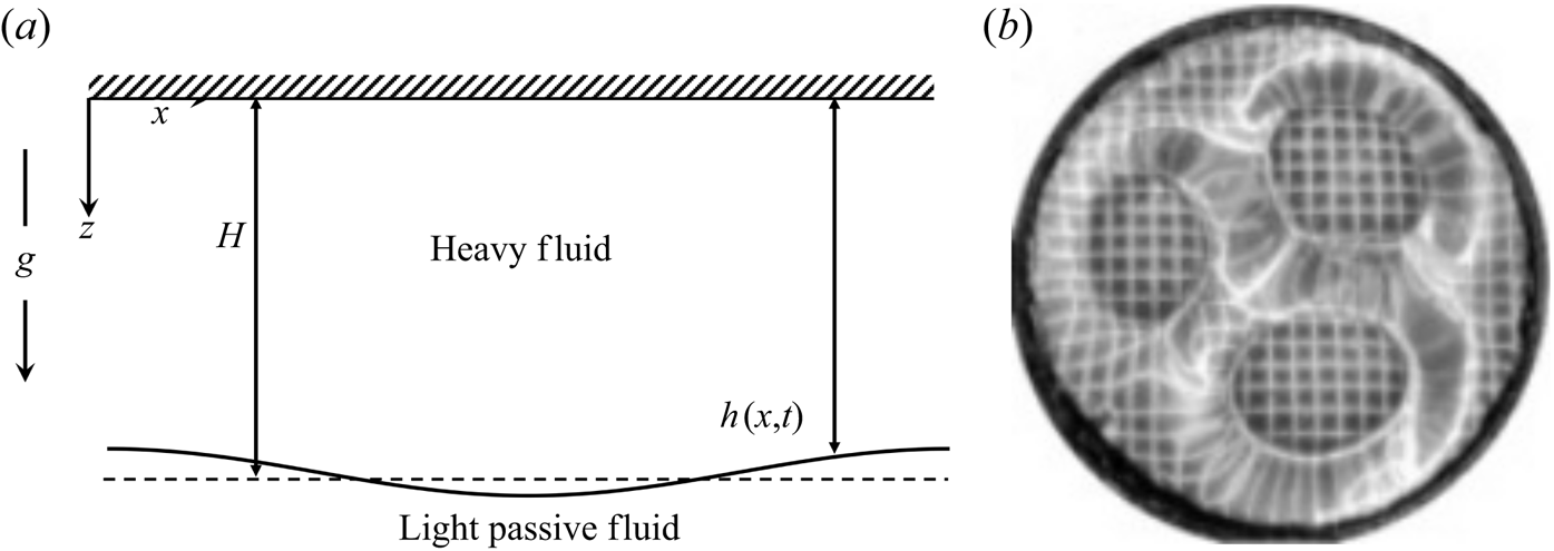
Figure 1. (a) Schematic of a heavy fluid overlying a light fluid under gravity. (b) Steady patterns observed at the free surface of a gravitationally unstable aqueous polyacrylamide soft gel. (From Mora et al. (Reference Mora, Phou, Fromental and Pomeau2014); republished with permission from the American Physical Society.)

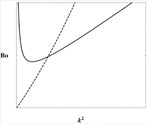
The only dimensionless group that determines the critical width, or the critical wavenumber, is the Bond number. This group, which will be formally introduced in § 3, reflects the balance between gravity and surface tension effects. The critical Bond number versus scaled wavenumber plot for the RT problem of non-elastic fluids is universal and is depicted as a straight line with unit slope and zero intercept in figure 2, denoted RT non-elastic limit. Such a plot, being monotonic, implies that there are no competing effects with wavenumber. At sufficiently small wavenumbers, surface tension effects are negligible compared to gravitational effects. At large wavenumbers, surface tension plays a strong stabilizing effect and overwhelms the destabilizing pressure gradients between crests and troughs at the interface. It is apparent from the straight line on figure 2 that the critical Bond number for neutral stability decreases to zero as the layer becomes infinitely wide. Any laterally constrained vessel will lead to critical conditions determined by the figure. Past work reveals that the nature of the instability at any point along the line in figure 2 is subcritical. This means that, beyond neutral stability, the interface proceeds towards rupture. This has been shown by experiments (Ratafia Reference Ratafia1973; Dalziel Reference Dalziel1993; Ramaprabhu & Andrews Reference Ramaprabhu and Andrews2004; Olson & Jacobs Reference Olson and Jacobs2009; Andrews & Dalziel Reference Andrews and Dalziel2010) and by theoretical predictions (Pullin Reference Pullin1982; Tryggvason Reference Tryggvason1988; Yiantsios & Higgins Reference Yiantsios and Higgins1989; Newhouse & Pozrikidis Reference Newhouse and Pozrikidis1990; Elgowainy & Ashgriz Reference Elgowainy and Ashgriz1997; Forbes Reference Forbes2009).

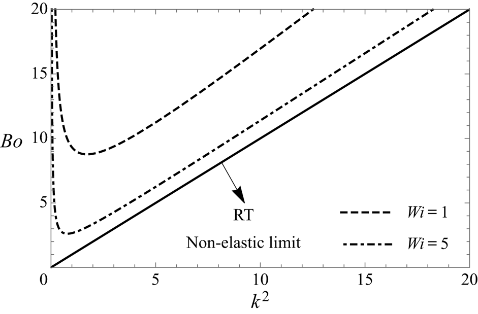
Figure 2. A typical plot of Bond number $(Bo)$ versus the square of the wavenumber $(k^{2})$ for the RT instability of a viscoelastic fluid. Weissenberg numbers $(Wi)$ are equal to 1 and 5, respectively, as shown. The Weissenberg number is the ratio of the elastic stresses to the viscous stresses and is defined later in table 2. As the Weissenberg number increases, the curves approach the classical RT instability limit (black solid line).

The RT problem changes character in a dramatic and substantive way when the heavy fluid is replaced by a soft gel, i.e. a viscoelastic fluid. Pattern formation at the free surface of a viscoelastic fluid is of relevance in the design of soft devices with tuneable shapes (Riccobelli & Ciarletta Reference Riccobelli and Ciarletta2017; Marthelot et al. Reference Marthelot, Strong, Reis and Brun2018) and also in the dynamics of mucus films in pulmonary capillaries (Dietze & Ruyer-Quil Reference Dietze and Ruyer-Quil2015). Examples of such materials are polyacrylamide and polydimethylsiloxane (PDMS). They are different from typical viscous fluids in that they bear both viscous as well as elastic character. We shall see in the next section that, at neutral stability, while velocity perturbations vanish as before, a viscoelastic fluid displays perturbations in displacement fields and the critical Bond number versus wavenumber plot is no longer a straight line, but displays a minimum as depicted in two different curves in figure 2. The critical Bond number and wavenumber relationship depends strongly on the elastic nature, now characterized by a new dimensionless group – the Weissenberg number – that shows the effect of elastic versus viscous stresses. This means that there are competitive effects with respect to the wavenumber of a disturbance for the case of RT instability of a viscoelastic fluid. The explanation for the occurrence of a minimum is that, while at low wavenumbers surface tension is weak as before, elastic stabilization retains its importance combating the destabilization driven by gravity. At high wavenumbers, in addition to the dissipation of pressure perturbations generated by elastic stresses, surface tension also acts to thwart the destabilization induced by gravity. This competition yields a wavenumber selection for which an unbounded layer displays patterns at the free surface. Interestingly, the shapes of the non-monotonic curves in figure 2 resemble those seen in the Bénard problem, where, in that case, the characteristic plot is the Rayleigh number versus the wavenumber and where the instability is always supercritical in nature (Joseph Reference Joseph1976). Contrast this with the RT problem for a non-viscoelastic fluid, where the critical Bond number for an infinitely wide container is zero and only a constrained vessel will lead to a critical Bond number under neutral conditions.

As the present study is focused on RT instability of viscoelastic fluids, we set our work in the context of previous research by reviewing earlier works that are directly pertinent to this study. In some of these studies, experiments were performed in large-aspect-ratio geometries, i.e. large horizontal-length-to-depth ratio, and the resulting planforms were steady hexagonal patterns implying saturated states upon instability (Mora et al. Reference Mora, Phou, Fromental and Pomeau2014; Chakrabarti et al. Reference Chakrabarti, Mora, Richard, Phou, Fromental, Pomeau and Audoly2018). These experiments were carried out in wide cylindrical and rectangular containers whose aspect ratios varied between 3 and 20. The typical physical properties of the viscoelastic fluid used in these experiments are given in table 1. Linear stability theories by these authors assumed a neo-Hookean model and curves similar to figure 2 were obtained. Capillary effects were ignored, and so the dip in the curves results from the competition between the low-wavenumber stability due to elastic normal stresses and large-wavenumber stability due to transverse dissipation of elastic stresses. Experiments by these authors were compared with theoretical predictions. Specifically, weak nonlinear analysis about the threshold wavenumber showed that hexagons were the most stable patterns to several waveform disturbances and that the bifurcation is transcritical for hexagonal patterns (cf. Chakrabarti et al. Reference Chakrabarti, Mora, Richard, Phou, Fromental, Pomeau and Audoly2018).

Table 1. Physical properties of polyacrylamide viscoelastic fluid (Müller & Zimmermann Reference Müller and Zimmermann1999; Mora et al. Reference Mora, Phou, Fromental and Pomeau2014).

Experiments in small-aspect-ratio containers were carried out by Yue et al. (Reference Yue, Yang, Yuhang and Shengqiang2019). In their study, the aspect ratio of the containers was between $0.4$ and $2$. These experiments showed the formation of non-axisymmetric modes at the free surface. For small aspect ratios, the instability was seen to be subcritical, with interface rupture, while for large aspect ratios, the instability saturated to a steady pattern. Finite-element simulations (Riccobelli & Ciarletta Reference Riccobelli and Ciarletta2017; Yue et al. Reference Yue, Yang, Yuhang and Shengqiang2019) have qualitatively predicted the patterns that were observed in experiments and have shown that the free surface saturates in large-aspect-ratio containers. As capillary effects have been ignored in the above works, the companion models can never approach the RT problem of a non-elastic fluid in the high-Weissenberg-number limit.

The observations from past work (Mora et al. Reference Mora, Phou, Fromental and Pomeau2014; Riccobelli & Ciarletta Reference Riccobelli and Ciarletta2017; Chakrabarti et al. Reference Chakrabarti, Mora, Richard, Phou, Fromental, Pomeau and Audoly2018; Yue et al. Reference Yue, Yang, Yuhang and Shengqiang2019) encourage us to hypothesize that there ought be a supercritical to subcritical transition at some wavenumber that depends on the Weissenberg number and where surface tension effects also play a role. Knowing this is important because such a transition tells us when we might expect to see an instability that saturates to steady wave patterns and when we might expect to see an instability that could ultimately lead to rupture. To find the transition from super- to subcritical states requires us to consider a weak nonlinear analysis about the critical or neutral state, where the Bond number is advanced slightly beyond its critical value.

In contrast with earlier works, the focus of this paper is to provide the physical rationale for the subcritical to supercritical transition in RT instability of viscoelastic fluids. In doing so, we obtain an analytical formula for a model problem that helps us to glean the physics of the transition. Keeping this in mind, our work focuses on linear viscoelastic models. Nonlinear constitutive equations are admittedly of practical consequence. However, insights into the competing effects of gravity, elasticity of the viscoelastic fluid and surface tension can be provided through the linear and weak nonlinear analysis using simple constitutive models.

The mathematical model for the instability of the viscoelastic medium is briefly explained in § 2. It is followed by a description of the linear stability analysis (§ 3) and by the necessary steps involved in the weak nonlinear analysis (§ 4). Details that involve cumbersome algebra are given as supplementary material to this paper (available at https://doi.org/10.1017/jfm.2021.80). To arrive at a simple formula that is descriptive of the problem, an idealized case of a two-dimensional (2-D) geometry is considered in § 4.1 and its three-dimensional (3-D) extension is given in § 4.2. Comments on the nature of the bifurcation for hexagonal and circular disturbances are made at the end of § 4.2; and key conclusions are summarized in § 5. We now turn to the mathematical model.

2. Mathematical model

The model assumes a hydrodynamically active viscoelastic fluid with constant properties overlying a passive gas in a destabilizing gravitational field, as depicted in figure 1(a). The fluid is taken to be linearly viscoelastic for algebraic simplicity whilst retaining essential physics in this study.

Now, the stress tensor in a viscoelastic fluid may be expressed in terms of the displacement field. The displacement vector, $\boldsymbol {R}$, is the displacement of the position vector, $\boldsymbol {x}$, in the current configuration from the position vector, $\boldsymbol {\zeta }$, in the reference configuration (cf. figure 3). In other words,

(2.1)\begin{equation} \boldsymbol{x}=\boldsymbol{\zeta}+\boldsymbol{R}(\boldsymbol{x}). \end{equation}

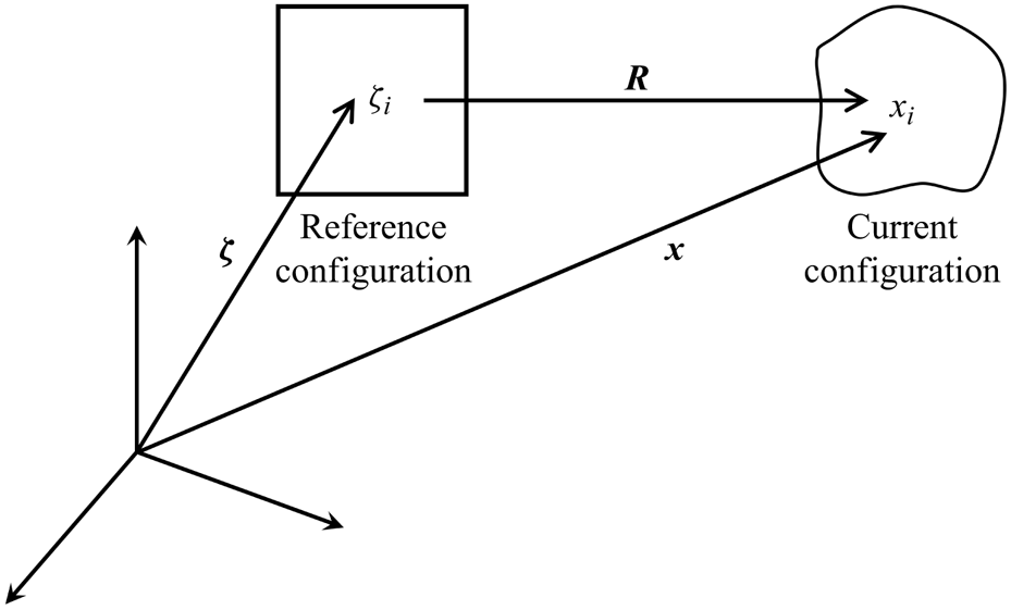
Figure 3. A depiction of a viscoelastic fluid in its reference configuration, and its current configuration, upon perturbation. The position vector of a point in the reference configuration is denoted $\boldsymbol {\zeta }$. The reference configuration is mapped to a point in the current configuration with a position vector $\boldsymbol {x}$.

For a linear viscoelastic fluid (cf. Landau & Lifshitz Reference Landau and Lifshitz1989; Shankar & Kumaran Reference Shankar and Kumaran2000; Dinesh & Pushpavanam Reference Dinesh and Pushpavanam2017) the stress tensor, $\boldsymbol{\mathsf{T}}$, is given by

(2.2)\begin{equation} \boldsymbol{\mathsf{T}} ={-}p \,\boldsymbol{\mathsf{I}} +G (\boldsymbol{\nabla}\boldsymbol{R} +\boldsymbol{\nabla}\boldsymbol{R}^{ \rm T} ) +\mu_g (\boldsymbol{\nabla}\boldsymbol{v} +\boldsymbol{\nabla}\boldsymbol{v}^{ \rm T} ). \end{equation}

Here $G$ and $\mu _g$ are the shear modulus and viscosity of the fluid material and $\boldsymbol {v}$ is the velocity field. Now the velocity field in the fluid is itself expressed in terms of the displacement field (cf. Patne, Giribabu & Shankar (Reference Patne, Giribabu and Shankar2017) for a detailed explanation). This expression is given by

(2.3)\begin{equation} \boldsymbol{v} =( \boldsymbol{\mathsf{I}}-\boldsymbol{\nabla}{\boldsymbol{R}}^\textrm{T})^{{-}1} \boldsymbol{\cdot}\frac{\partial{\boldsymbol{R}}}{\partial{t}}. \end{equation}

The equations of motion in the viscoelastic medium are thus

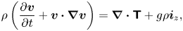(2.4)\begin{equation} \rho\left(\frac{\partial\boldsymbol{v}}{\partial t} +\boldsymbol{v}\boldsymbol{\cdot}\boldsymbol{\nabla}{\boldsymbol{v}}\right) =\boldsymbol{\nabla}\boldsymbol{\cdot} \boldsymbol{\mathsf{T}} +g\rho\boldsymbol{i}_{ {z}}, \end{equation}

where $\boldsymbol{\mathsf{T}}$ and $\boldsymbol {v}$ are given by (2.2) and (2.3), where in (2.3) the superscript T on $\boldsymbol {\nabla } \boldsymbol {R}$ is the transpose of the tensor $\boldsymbol {\nabla } \boldsymbol {R}$ and $\boldsymbol{\mathsf{I}}$ is the identity tensor, and where $\boldsymbol {i}_{{z}}$ is the base vector in the positive $z$-direction in (2.4). The horizontal and vertical components of the displacement vector, $\boldsymbol {R}$, are denoted by $X$ and $Z$, respectively.

The viscoelastic fluid is taken to be incompressible and the mass conservation demands (Howell, Kozyreff & Ockendon Reference Howell, Kozyreff and Ockendon2009; Patne et al. Reference Patne, Giribabu and Shankar2017)

(2.5)\begin{equation} \det(\boldsymbol{\mathsf{F}})=1, \end{equation}

where $\boldsymbol{\mathsf{F}}$ is the deformation tensor given by $\boldsymbol{\mathsf{F}}={\partial \zeta _i}/{\partial x_j}$. Here $\zeta _i$ represent the components of the position vector in the reference configuration. Upon expansion of (2.5) and using (2.1) we get

(2.6)\begin{equation} \frac{\partial X}{\partial x}+\frac{\partial Z}{\partial z}-\frac{\partial X}{\partial x} \frac{\partial Z}{\partial z}+\frac{\partial Z}{\partial x} \frac{\partial X}{\partial z}=0. \end{equation}

Equations (2.4) and (2.6) along with the representations for $\boldsymbol{\mathsf{T}}$ and $\boldsymbol {v}$ constitute the domain equations. These are complemented by boundary conditions at the rigid wall and at the interface.

At the wall, the displacement fields are taken to be zero. At the interface, $z=h(x,t)$, the normal and the tangential components of the momentum balance hold. They are

(2.7a,b)\begin{equation} \boldsymbol{n} \boldsymbol{\cdot} \boldsymbol{\mathsf{T}}\boldsymbol{\cdot} {\boldsymbol{t}}= 0 \quad \mbox{and} \quad {\boldsymbol{n}}\boldsymbol{\cdot} \boldsymbol{\mathsf{T}}\boldsymbol{\cdot}{\boldsymbol{n}}={-}\gamma \boldsymbol{\nabla} \boldsymbol{\cdot} \boldsymbol{n}, \end{equation}

where the unit normal vector $({\boldsymbol {n}})$ and the unit tangent vector $({\boldsymbol {t}})$ are given by

(2.8a,b)\begin{equation} \boldsymbol{n} = \frac{-\dfrac{\partial h}{\partial x} \boldsymbol{i}_{x}+\boldsymbol{i}_{z}}{\left[1+\left(\dfrac{\partial h}{\partial x}\right)^{2}\right]^{1/2}}\quad \mbox{and} \quad \boldsymbol{t} = \frac{\boldsymbol{i}_{x}+\dfrac{\partial h}{\partial x} \boldsymbol{i}_{z}}{\left[1+\left(\dfrac{\partial h}{\partial x}\right)^{2}\right]^{1/2}}. \end{equation}

In addition we have an impermeable interface along with its kinematic relation

(2.9)\begin{equation} \boldsymbol{v} \boldsymbol{\cdot} \boldsymbol{n} = \frac{\dfrac{\partial h}{\partial t}}{\left[1+\left(\dfrac{\partial h}{\partial x}\right)^{2}\right]^{1/2}}. \end{equation}

The governing equations are made dimensionless by using the following scales denoted by the subscript ‘c’:

(2.10a–f)\begin{equation} x_{c}=H,\quad z_{c}=H,\quad X_{c}=H,\quad Z_{c}=H,\quad t_{c}=\frac{H}{U},\quad p_{c}=\frac{\mu U}{H}. \end{equation}

Here $U$ is a characteristic velocity scale. Using the above scales, the non-dimensional model is now given by

(2.11)\begin{equation} Re \left(\frac{\partial\boldsymbol{v}}{\partial t} +\boldsymbol{v}\boldsymbol{\cdot}\boldsymbol{\nabla}{\boldsymbol{v}}\right) ={-}\boldsymbol{\nabla}p+\frac{1}{Wi} \nabla^{2} \boldsymbol{R} +\frac{1}{Wi}\boldsymbol{\nabla} (\boldsymbol{\nabla} \boldsymbol{\cdot} \boldsymbol{R} )+\nabla^{2} \boldsymbol{v} +\frac{Bo}{Ca} \boldsymbol{i}_{ {z}}, \end{equation}

where $Wi={\mu U}/{G H}$, 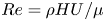$Re={\rho H U}/{\mu }$, 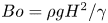$Bo={\rho g H^{2}}/{\gamma }$ and $Ca={\mu U}/{\gamma }$. The mass conservation equation (2.6) remains unchanged and does not induce any dimensionless groups. The interfacial force balance conditions at $z = h(x,t)$ become

(2.12a,b)\begin{equation} \boldsymbol{n} \boldsymbol{\cdot} \boldsymbol{\mathsf{T}}\boldsymbol{\cdot}\boldsymbol{t}= 0 \quad \mbox{and} \quad \boldsymbol{n}\boldsymbol{\cdot} \boldsymbol{\mathsf{T}}\boldsymbol{\cdot}\boldsymbol{n} ={-}\frac{1}{Ca}\,\boldsymbol{\nabla} \boldsymbol{\cdot} \boldsymbol{n}. \end{equation}

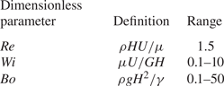
Four key dimensionless groups $Re$, $Ca$, $Bo$ and $Wi$ emerge from the scaling of the governing equations and the boundary conditions. They may be calculated for typical thermophysical properties as depicted in table 1 and shown in table 2. A base solution to equations (2.6), (2.11) and (2.12a,b) are $\boldsymbol {R}$, $\boldsymbol {v}$ and $\boldsymbol{\mathsf{T}}$ equal to zero. Our goal is to determine the stability of the base solution and inspect the nature of the bifurcation as we advance a control parameter from the bifurcation point. To this end, we must look for neutral stability conditions and then consider the steady-state nature of the branching, observing that $Wi$, $Ca$ and $Bo$ are the only pertinent dimensionless groups of the problem. Under steady-state conditions it ought to be noted that the capillary number, $Ca$, always appears as ${Ca}/{Wi}$ and therefore a velocity scale, $U$, need not be specified or equivalently one may choose $U$ such that $Ca$ is taken to be unity without any loss of generality.

Table 2. Ranges of key dimensionless quantities for polyacrylamide viscoelastic fluid. The velocity scale $U$ is based on the capillary number such that $U={\gamma }/{\mu }$.

3. Linear stability analysis

Linear stability analysis of the problem is performed by introducing small perturbations, $\boldsymbol {R}^{{\star }}$ and $\boldsymbol {v}^{{\star }}$, via

(3.1)\begin{equation} \boldsymbol{R} (x,z,t )= \boldsymbol{R}_0+ \boldsymbol{R}^{ {\star}}(z) \exp({(\sigma t+\textrm{i}kx )}) \end{equation}

and

(3.2)\begin{equation} \boldsymbol{v}=\boldsymbol{v}^{ {\star}}, \end{equation}

where $\boldsymbol {R}_{{0}}$ is the base-state displacement field in the viscoelastic fluid and $\boldsymbol {R}-\boldsymbol {R}_{{0}}$ is an infinitesimal disturbance, and where $\boldsymbol {v}^{{\star }}= {\partial \boldsymbol {R}^{{\star }}}/{\partial t}$. The disturbances considered in (3.1) are taken to be 2-D in space, i.e. functions of $z$ and $x$ only. Extensions to three dimensions are given for the case of square disturbances later and it will be seen that inferences drawn from the corresponding analysis do not change qualitatively. We therefore restrict ourselves to 2-D disturbances for the sake of simplicity in the majority of this study.

Equation (3.1) will lead to linearized equations on the reference domain, ($\zeta _x$, $\zeta _z$) (cf. Johns & Narayanan Reference Johns and Narayanan2002). In the analysis that follows, all perturbed equations are valid only in the reference domain, where we denote the coordinates $x$ and $z$ for convenience instead of $\zeta _x$ and $\zeta _z$. Observe that $\boldsymbol {R}_{0}=\boldsymbol {0}$ and the base-state pressure gradient is thus balanced by the gravitational body force, i.e.

(3.3)\begin{equation} \frac{\textrm{d}p_{0}}{\textrm{d}z}=Gr=\frac{Bo}{Ca}, \end{equation}

where $Gr={\rho g H^{2}}/{\mu U}$. The linearized equations after substituting the form of the perturbations given by (3.1) become

(3.4)\begin{gather} \textrm{i}kX^{{\star}}+\frac{\textrm{d}Z^{{\star}}}{\textrm{d} z}=0, \end{gather}

(3.5)\begin{gather}Re\,\sigma^{2} X^{{\star}}={-} \textrm{i}kp^{{\star}}+ \left(\frac{1}{Wi}+\sigma\right) \left(\frac{\textrm{d}^2 X^{{\star}}}{\textrm{d}z^2}-k^{2}X^{{\star}}\right), \end{gather}

(3.6)\begin{gather}Re\,\sigma^{2} Z^{{\star}}={-} \frac{\textrm{d}p^{{\star}}}{\textrm{d}z}+ \left(\frac{1}{Wi}+\sigma\right) \left(\frac{\textrm{d}^2 Z^{{\star}}}{\textrm{d} z^2}-k^{2}Z^{{\star}}\right). \end{gather}

Linearizing the boundary conditions (2.9) and (2.12a,b) at the reference interface, $z=1$, gives

(3.7)\begin{gather} v^{{\star}}_{z}=\sigma Z^{{\star}}=\sigma h^{{\star}}, \quad \mbox{i.e.} \ Z^{{\star}}= h^{{\star}}, \end{gather}

(3.8)\begin{gather}\left(\frac{1}{Wi}+\sigma\right) \left(\frac{\textrm{d} X^{{\star}}}{\textrm{d} z}+\textrm{i}kZ^{{\star}}\right)=0 \end{gather}

and

(3.9)\begin{equation} -p^{{\star}}- \frac{Bo}{Ca}\,h^{{\star}}+2 \left(\frac{1}{Wi}+\sigma\right)\frac{\textrm{d} Z^{{\star}}}{\textrm{d} z}={-}\frac{k^{2} h^{{\star}}}{Ca}. \end{equation}

The stability of this problem is determined by (3.4)–(3.6) and the boundary conditions (3.7)–(3.9). The growth rate of the perturbations, $\sigma$, is a function of $Re$, $Ca$, $Bo$, $Wi$ and $k$, and determined by an eigenvalue problem of the form

(3.10)\begin{equation} \boldsymbol{\mathsf{A}}x=\sigma \boldsymbol{\mathsf{B}}x. \end{equation}

These linearized equations are solved using a Chebyshev collocation technique (Guo, Labrosse & Narayanan Reference Guo, Labrosse and Narayanan2013) for a range of $k$. The growth rate $\sigma$ of the perturbations is depicted graphically in figure 4 for typical values of $Re$, ${Bo}/{Ca}$ and $Wi$.

Figure 4. Plots of $\sigma$ versus $k^{2}$ obtained from linear stability for $Wi= 0.5$, $1$ and 5, $Gr={Bo}/{Ca}=20$ and $Re \simeq 2$.

Several observations may be made. First, the growth constant starts negative at $k^{2}=0$, rises, reaches a maximum and then decreases. Second, for small $Wi$, the growth rate is always negative, indicating the strongly stabilizing nature of the elasticity. As $Wi$ increases, $\sigma$ can become zero, then positive, before descending to zero again, thereby showing the presence of two neutral points. Clearly, there is a critical value of $Wi$ for the input $Re$, $Bo$ and $Ca$ at which the two neutral points coincide at the maximum. This leads to a neutral curve as depicted in figure 2. Finally, as $Wi$ becomes very large, the $\sigma$ versus $k^{2}$ curve approaches the RT limit, as the models become the same.

To understand the nature of the initial rise and subsequent fall in the $\sigma$ versus $k^{2}$ curve, we consider a heuristic model from which an analytical expression for $\sigma$ can be obtained. This happens when the domain dynamics are dropped but interface dynamics are retained only in the normal component of the force balance. Admittedly, this is a heuristic model, but we pursue it with the expectation that we can learn why the growth rate commences negative when $k\to 0$. The normal component of the force balance then attains the following form at the interface, $z=1$:

(3.11)\begin{align} \sigma \left[-\left(\frac{\textrm{d}^{3}Z^{{\star}}}{\textrm{d}z^{3}}-3k^{2}\frac{\textrm{d}Z^{{\star}}}{\textrm{d}z}\right)\right]={-} \frac{k^{4}h^{{\star}}}{Ca}+k^{2}\frac{Bo}{Ca}h^{{\star}} -\frac{1}{Wi}\left[-\left(\frac{\textrm{d}^{3}Z^{{\star}}}{\textrm{d}z^{3}}- 3k^{2}\frac{\textrm{d}Z^{{\star}}}{\textrm{d}z}\right)\right]. \end{align}

In (3.11), $Z^{\star }$ and its derivatives are obtained by solving the domain equations subject to the assumptions in our heuristic model and evaluated at $z=1$. For $k^{2}=0$, the expression asymptotically simplifies to

(3.12)\begin{equation} \sigma={-}\frac{1}{Wi}. \end{equation}

It can be shown that the bracketed term on the left-hand side of (3.11) is positive while the first and last terms of the right-hand side are negative and the middle term is positive. This shows that the stabilizing feature at $k^{2}\to 0$ is entirely due to the elastic effect while the rise is due to gravity given by $Bo$ in (3.11) and the final fall is due to the capillary effect.

We now return to the full model where neutral stability is addressed. Here dynamics are no longer of concern and the full physics of the model are retained. To determine the conditions for neutral stability, we set $\sigma$ to zero by observing that exchange of stability holds. A proof of this is available in appendix A, where it is also shown that velocity perturbations for neutral conditions are zero.

Under neutral conditions, equation (3.11) becomes

(3.13)\begin{align} Bo&=\frac{k [4 Ca\, k^2+2 Ca \cosh (2 k)+2 Ca-2 k^2 Wi+k Wi \sinh (2 k)]}{Wi [\sinh (2 k)-2k]} \nonumber\\ &=\frac{2 Ca \,k [2 k^2+ \cosh (2 k)+1]}{Wi [\sinh (2 k)-2k]}+k^2. \end{align}

Clearly, $Re$ plays no role under neutral conditions and the neutral curve is given by $Bo$ versus $k^{2}$ with $Wi$ as a parameter. The typical neutral stability curves in the $Bo$ versus $k^{2}$ parameter space are shown in figure 2. The solid line in figure 2 represents the $Bo$ versus $k^{2}$ trend for a non-elastic fluid. As $Wi$ tends to infinity, the viscoelastic fluid behaves like a non-elastic liquid. It is seen from (3.13) that $Wi$ must approach infinity via at least $\textit{O}(1/k^3)$ in order that $Bo$ increase monotonically with $k^2$.

Decreasing $Wi$ from the large-$Wi$ limit leads to departure from non-elastic behaviour, and at $Wi=0$ the medium acts like an elastic solid, making the system completely stable. This trend is seen in the curves for $Wi = 1$ and 5 in figure 2. Also observe that, with a decrease of $Wi$ from the large-$Wi$ limit, the curves take on the character of classical hydrodynamic instability problems such as the Bénard problem of convection. This urges us to think that, for large $Wi$, the instability will be subcritical like the RT instability of a non-elastic fluid, and for decreasing $Wi$, the instability will become supercritical like the Bénard problem. To find out the nature of the bifurcation, we carry out a weak nonlinear analysis near the bifurcation point.

4. Weak nonlinear analysis and discussion

Anticipating a pitchfork-shaped branch, we advance $Bo$ from its critical value by an amount, $\epsilon$, such that $\epsilon$ is defined by

(4.1)\begin{equation} {} Bo=Bo_{0}+\frac{\epsilon^{2}}{2}. \end{equation}

In response to this increase in $Bo$, the displacement fields, pressure field and the surface elevation change from their base state by

(4.2)\begin{gather} X(x,z)=X_0+\epsilon X_{1}(x,z)+\frac{\epsilon^{2}}{2} X_{2}(x,z)+\frac{\epsilon^{3}}{6} X_{3}(x,z)+\cdots, \end{gather}

(4.3)\begin{gather}Z(x,z)=Z_0+\epsilon Z_{1}(x,z)+\frac{\epsilon^{2}}{2} Z_{2}(x,z)+\frac{\epsilon^{3}}{6} Z_{3}(x,z)+\cdots, \end{gather}

(4.4)\begin{gather}p(x,z)=p_0+\epsilon p_{1}(x,z)+\frac{\epsilon^{2}}{2} p_{2}(x,z)+\frac{\epsilon^{3}}{6} p_{3}(x,z)+\cdots \end{gather}

and

(4.5)\begin{equation} h(x)=h_0+\epsilon h_{1}(x)+\frac{\epsilon^{2}}{2} h_{2}(x)+\frac{\epsilon^{3}}{6} h_{3}(x)+\cdots. \end{equation}

At the free surface, the interior displacement field, $X$, is expressed as (Johns & Narayanan Reference Johns and Narayanan2002)

(4.6)\begin{align} X(x,z)&=X_0+\epsilon \left(X_{1}+h_{1}\frac{\partial X_{0}}{\partial z}\right)+\frac{\epsilon^{2}}{2} \left(X_{2}+h_{2}\frac{\partial X_{0}}{\partial z}+2h_{1}\frac{\partial X_{1}}{\partial z}+h_{1}^{2}\frac{\partial^{2} X_{0}}{\partial z^{2}}\right)\nonumber\\ &\quad +\frac{\epsilon^{3}}{6} \left(X_{3}+h_{3}\frac{\partial X_{0}}{\partial z}+3h_{2}\frac{\partial X_{1}}{\partial z}+3h_{1}\frac{\partial X_{2}}{\partial z}+3h_{1}h_{2}\frac{\partial^{2} X_{0}}{\partial z^{2}}\right.\nonumber\\ &\quad \left.+ \, 3h_{1}^{2}\frac{\partial^{2} X_{1}}{\partial z^{2}}+h_{1}^{3}\frac{\partial^{3} X_{0}}{\partial z^{3}}\right)+\cdots, \end{align}

and likewise for $Z(x,z)$ and $p(x,z)$. The equations at various orders can thus be obtained.

The equations at $\textit{O}(\varepsilon )$ are given by

(4.7)\begin{gather} \frac{\partial X_{1}}{\partial x}+\frac{\partial Z_{1}}{\partial z}=0, \end{gather}

(4.8)\begin{gather}- \frac{\partial p_{1}}{\partial x}+ \frac{1}{Wi} \left(\frac{\partial ^2X_{1}}{\partial x^2}+\frac{\partial ^2X_{1}}{\partial z^2}\right)=0, \end{gather}

(4.9)\begin{gather}- \frac{\partial p_{1}}{\partial z}+ \frac{1}{Wi} \left(\frac{\partial ^2Z_{1}}{\partial x^2}+\frac{\partial ^2Z_{1}}{\partial z^2}\right)=0. \end{gather}

The boundary conditions at $\textit{O}(\varepsilon )$ at the rigid wall, i.e. $z=0$, are

(4.10a,b)\begin{equation} {} Z_{1}=0 \quad \mbox{and}\quad X_{1}=0. \end{equation}

The interfacial conditions, i.e. at $z=1$, at $\textit{O}(\varepsilon )$ become

(4.11)\begin{gather} Z_{1}-h_{1}=0, \end{gather}

(4.12)\begin{gather}\frac{1}{Wi} \left(\frac{\partial X_{1}}{\partial z}+\frac{\partial Z_{1}}{\partial x}\right)=0 \end{gather}

and

(4.13)\begin{equation} -p_{1}- \frac{Bo_{0}}{Ca}\,h_{1}+\frac{2}{Wi}\frac{\partial Z_{1}}{\partial z}-\frac{1}{Ca}\frac{\partial ^2h_{1}}{\partial x^2}=0. \end{equation}

Observe that the $\textit{O}(\epsilon )$ equations are precisely the neutral stability equations. Hence $h_{1}(x)$ becomes $h_{1}(x)=\mathcal {A}\cos (k x)$. Our job now is to determine the sign of $\mathcal {A}^{2}$, noting that a positive value of $\mathcal {A}^{2}$ implies a supercritical bifurcation and a negative value implies a subcritical bifurcation. To determine $\mathcal {A}^{2}$ we proceed to the next order.

The governing equations at $\textit{O}({\varepsilon ^{2}}/{2})$ are given by

(4.14)\begin{gather} \frac{\partial X_{2}}{\partial x}+\frac{\partial Z_{2}}{\partial z}=2\frac{\partial X_{1}}{\partial x}\frac{\partial Z_{1}}{\partial z}-2\frac{\partial X_{1}}{\partial z}\frac{\partial Z_{1}}{\partial x}, \end{gather}

(4.15)\begin{gather}- \frac{\partial p_{2}}{\partial x}+ \frac{1}{Wi} \left(\frac{\partial ^2X_{2}}{\partial x^2}+\frac{\partial ^2X_{2}}{\partial z^2}\right)=\frac{-1}{Wi}\frac{\partial}{\partial x}\left(2\frac{\partial X_{1}}{\partial x}\frac{\partial Z_{1}}{\partial z}-2\frac{\partial X_{1}}{\partial z}\frac{\partial Z_{1}}{\partial x}\right) \end{gather}

and

(4.16)\begin{equation} {-}\frac{\partial p_{2}}{\partial z}+ \frac{1}{Wi} \left(\frac{\partial ^2Z_{2}}{\partial x^2}+\frac{\partial ^2Z_{2}}{\partial z^2}\right)={-}1-\frac{1}{Wi}\frac{\partial}{\partial z}\left(2\frac{\partial X_{1}}{\partial x}\frac{\partial Z_{1}}{\partial z}-2\frac{\partial X_{1}}{\partial z}\frac{\partial Z_{1}}{\partial x}\right). \end{equation}

The boundary conditions at $z=0$ are

(4.17a,b)\begin{equation} Z_{2}=0\quad \mbox{and} \quad X_{2}=0. \end{equation}

The interfacial conditions, i.e. at $z=1$, are now

(4.18)\begin{gather} Z_{2}-h_{2}={-}2h_{1}\frac{\partial Z_{1}}{\partial z}, \end{gather}

(4.19)\begin{gather}\frac{1}{Wi} \left(\frac{\partial X_{2}}{\partial z}+\frac{\partial Z_{2}}{\partial x}\right)=\frac{-4}{Wi}\frac{\partial h_{1}}{\partial x}\frac{\partial Z_{1}}{\partial z}+\frac{4}{Wi}\frac{\partial h_{1}}{\partial x}\frac{\partial X_{1}}{\partial x}-\frac{2h_{1}}{Wi}\frac{\partial ^2X_{1}}{\partial z^2}-\frac{2h_{1}}{Wi}\frac{\partial ^2Z_{1}}{\partial z \partial x} \end{gather}

and

(4.20)\begin{align} &{-}p_{2}- \frac{Bo_{0}}{Ca}\,h_{2}+\frac{2}{Wi}\frac{\partial Z_{2}}{\partial z} -\frac{1}{Ca}\frac{\partial ^2h_{2}}{\partial x^2}\nonumber\\ & \quad =2h_{1}\frac{\partial p_{1}}{\partial z}-\frac{4h_{1}}{Ca}\frac{\partial^{2} Z_{1}}{\partial z^{2}} +\frac{4}{Wi} \frac{\partial h_{1}}{\partial x}\frac{\partial X_{1}}{\partial z}+\frac{4}{Wi} \frac{\partial h_{1}}{\partial x}\frac{\partial Z_{1}}{\partial x}. \end{align}

Observe the pattern of equations in (4.14)–(4.20) and compare them with (4.7)–(4.13). The right-hand sides compriseforcing terms that are quadratic combinations of $\textit{O}(\epsilon )$ terms and directly proportional to $\mathcal {A}^{2}$. We call these quadratic combinations $(1,1)$ terms due to their bilinear combinations of first-order variables. The solution to the second-order problem must therefore be the sum of several $\mathcal {A}^{2}$-dependent terms and a sole term independent of $\mathcal {A}$ due to the first term on the right-hand side of (4.16). Upon observing that (4.7)–(4.13) are homogeneous and employing solvability conditions on (4.14)–(4.20), we see that solvability of equations (4.14)–(4.20) is automatically satisfied. Thus we cannot determine $\mathcal {A}^{2}$ at this order and must advance to the next order.

The governing equations at $\textit{O}({\varepsilon ^{3}}/{6})$ are given by

(4.21)\begin{gather} \frac{\partial X_{3}}{\partial x}+\frac{\partial Z_{3}}{\partial z}=3\frac{\partial X_{1}}{\partial x}\frac{\partial Z_{2}}{\partial z}+3\frac{\partial X_{2}}{\partial x}\frac{\partial Z_{1}}{\partial z}-3\frac{\partial X_{2}}{\partial z}\frac{\partial Z_{1}}{\partial x}-3\frac{\partial X_{1}}{\partial z}\frac{\partial Z_{2}}{\partial x}, \end{gather}

(4.22)\begin{gather}- \frac{\partial p_{3}}{\partial x}+ \frac{1}{Wi} \left(\!\frac{\partial ^2X_{3}}{\partial x^2}+\frac{\partial ^2X_{3}}{\partial z^2}\!\right)=\frac{-3}{Wi}\frac{\partial }{\partial x}\left(\!\frac{\partial X_{1}}{\partial x}\frac{\partial Z_{2}}{\partial z}+\frac{\partial X_{2}}{\partial x}\frac{\partial Z_{1}}{\partial z}-\frac{\partial X_{2}}{\partial z}\frac{\partial Z_{1}}{\partial x}-\frac{\partial X_{1}}{\partial z}\frac{\partial Z_{2}}{\partial x}\!\right) \end{gather}

and

(4.23)\begin{equation} {-}\frac{\partial p_{3}}{\partial z}+ \frac{1}{Wi} \left(\frac{\partial ^2Z_{3}}{\partial x^2}+\frac{\partial ^2Z_{3}}{\partial z^2}\right)=\frac{-3}{Wi}\frac{\partial }{\partial z}\left(\!\frac{\partial X_{1}}{\partial x}\frac{\partial Z_{2}}{\partial z}+\frac{\partial X_{2}}{\partial x}\frac{\partial Z_{1}}{\partial z}-\frac{\partial X_{2}}{\partial z}\frac{\partial Z_{1}}{\partial x}-\frac{\partial X_{1}}{\partial z}\frac{\partial Z_{2}}{\partial x}\!\right). \end{equation}

The boundary conditions at $z=0$ are

(4.24a,b)\begin{equation} {} Z_{3}=0\quad \mbox{and} \quad X_{3}=0. \end{equation}

The interfacial conditions at $z=1$ are

(4.25)\begin{equation} Z_{3}-h_{3}={-}3h_{2}\frac{\partial Z_{1}}{\partial z}-3h_{1}\frac{\partial Z_{2}}{\partial z}-3h_{1}^{2}\frac{\partial^{2} Z_{1}}{\partial z^{2}}, \end{equation}

(4.26)\begin{align} \frac{1}{Wi} \left(\frac{\partial X_{3}}{\partial z}+\frac{\partial Z_{3}}{\partial x}\right)&=\frac{-6}{Wi}\frac{\partial h_{2}}{\partial x}\left(\frac{\partial Z_{1}}{\partial z}-\frac{\partial X_{1}}{\partial x}\right) -\frac{6}{Wi}\frac{\partial h_{1}}{\partial x}\left(\frac{\partial Z_{2}}{\partial z} -\frac{\partial X_{2}}{\partial x}\right)\nonumber\\ &\quad +\frac{12}{Wi}\left(\frac{\partial h_{1}}{\partial x}\right)^2\left(\frac{\partial X_{1}}{\partial z} +\frac{\partial Z_{1}}{\partial x}\right) -\frac{3h_{2}}{Wi}\left(\frac{\partial ^2X_{1}}{\partial z^2}+\frac{\partial ^2Z_{1}}{\partial z\partial x}\right)\nonumber\\ &\quad -\frac{3h_{1}}{Wi}\left(\frac{\partial ^2X_{2}}{\partial z^2}+\frac{\partial ^2Z_{2}}{\partial z\partial x}\right) -\frac{3h_{1}^{2}}{Wi}\left(\frac{\partial ^3X_{1}}{\partial z^3}+\frac{\partial ^3Z_{1}}{\partial z^2\partial x}\right)\nonumber\\ &\quad -\frac{12h_{1}}{Wi}\frac{\partial h_{1}}{\partial x}\left(\frac{\partial ^2Z_{1}}{\partial z^2}-\frac{\partial ^2X_{1}}{\partial z \partial x}\right) \end{align}

and

(4.27)\begin{align} & {-}p_{3}-\frac{Bo_{0}}{Ca}\,h_{3}+\frac{2}{Wi}\frac{\partial Z_{3}}{\partial z}-\frac{1}{Ca}\frac{\partial ^2h_{3}}{\partial x^2}\nonumber\\ &\quad =3h_{2}\frac{\partial p_{1}}{\partial z}+\boxed{3h_{1}\frac{\partial p_{2}}{\partial z}}+3h_{1}^{2}\frac{\partial^{2} p_{1}}{\partial z^{2}}\nonumber\\ &\qquad -\frac{6h_{2}}{Wi}\frac{\partial^{2} Z_{1}}{\partial z^{2}} -\frac{6h_{1}}{Wi}\frac{\partial^{2} Z_{2}}{\partial z^{2}}+\frac{6}{Wi}\frac{\partial h_{2}}{\partial x}\left(\frac{\partial X_{1}}{\partial z} +\frac{\partial Z_{1}}{\partial x}\right)\nonumber\\ &\qquad -\frac{12}{Wi}\left(\frac{\partial h_{1}}{\partial x}\right)^2\left(\frac{\partial X_{1}}{\partial x} -\frac{\partial Z_{1}}{\partial z}\right) +\frac{6}{Wi}\frac{\partial h_{1}}{\partial x}\left(\frac{\partial Z_{2}}{\partial x} +\frac{\partial X_{2}}{\partial z}\right)\nonumber\\ &\qquad +\frac{12h_{1}}{Wi}\frac{\partial h_{1}}{\partial x}\left(\frac{\partial ^2X_{1}}{\partial z^2}+\frac{\partial ^2Z_{1}}{\partial z \partial x}\right)-\frac{6h_{1}^{2}}{Wi}\frac{\partial^{3} Z_{1}}{\partial z^{3}} -\frac{9}{Ca}\left(\frac{\partial h_{1}}{\partial x}\right)^{2}\frac{\partial ^2h_{1}}{\partial x^2}. \end{align}

The forcing terms from (4.21)–(4.27) are bilinear combinations of second-order and first-order terms, i.e. $(2,1)$ terms, and trilinear combinations of first-order terms, i.e. $(1,1,1)$ terms. All of these terms are effectively homogeneous factors of $\mathcal {A}^3$, with the exception of the boxed term in (4.27), i.e. $3h_{1}({\partial p_{2}}/{\partial z})$. This term is special because it contains an $\textit{O}( \epsilon )$-independent part arising from the first term on the right-hand side of (4.16). This observation is important because it is the sole reason for us to be able to determine $\mathcal {A}^{2}$ upon employing solvability conditions on (4.21)–(4.27) using the first-order equations (4.7)–(4.13). Saturation at this order, i.e. being able to obtain $\mathcal {A}^{2}$ at this order, determines not only the amplitude but also the nature of the bifurcation.

If $\mathcal {A}^{2}$ is positive, the branch is supercritical, but if it is negative, the Bond number would not be advanced as indicated by (4.1) but reduced instead and the branch would become a subcritical pitchfork. The calculations that involve solvability require the use of symbolic manipulation, which was carried out in Mathematica $^{\circledR }$ and the details are provided in the supplementary material to this paper. The algebraic complications can be reduced if the nonlinear terms of equation (2.6) are dropped. It has been observed by the present authors that the results do not change qualitatively. The general results without making this approximation are depicted in figure 5. This figure is to be interpreted as follows. We first input $Wi$ and $Bo$ into equation (3.13) and calculate $k^{2}$. This is the critical value of $k^{2}$ and must be used in the weak nonlinear analysis from which the value of $\mathcal {A}^{2}$ is obtained. From this we learn that, for every input $Bo$ for a given $Wi$, the bifurcation corresponding to the critical $k^{2}$ is either supercritical or subcritical. It is apparent from figure 5(a) that the branching is supercritical for a large range of $k^{2}$ for moderate $Wi$. However, as $Wi$ becomes large, this range contracts and the branching becomes subcritical, indicating RT-type behaviour. Figure 5(b) depicts an example of the intersection of the transition curve with the neutral stability curve for $Wi=1$, where all accessible wavenumbers above the transition line lead to supercritical branching and all wavenumbers below the transition line lead to subcritical branching. A key observation is that the transition line intersects the neutral stability curve to the right of the minimum, thereby affording the possibility of supercritical saturated waves. To glean the physics of the transition, we turn to a simpler model of the problem, dropping the nonlinear term in (2.6) and taking the viscoelastic fluid depth to be infinite.

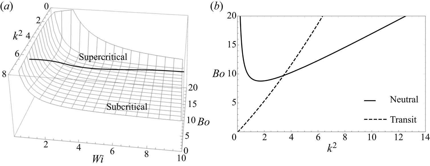
Figure 5. (a) Plots of $Bo$ versus $k^{2}$ versus $Wi$ obtained from the weak nonlinear analysis. The change in the sign of $\mathcal {A}^{2}$ is shown in the plot. (b) Plot of $Bo$ versus $k^{2}$ obtained from the neutral stability calculations (solid line) for $Wi=1.0$. The dashed line, from weak nonlinear calculations, demarcates the supercritical and subcritical transition. This is obtained by setting $\mathcal {A}^{2} = 0$ in the third-order calculations.

4.1. Tracing the cause of the transition from super- to subcritical branching

In the previous paragraphs, we observed that the nature of the bifurcation could be either supercritical or subcritical in nature. Here, our focus is on tracing the terms responsible for this transition. To accomplish this, we drop the nonlinear terms in (2.6) and carry out the weak nonlinear analysis of a viscoelastic fluid layer whose depth is infinite. This infinite layer configuration allows us to simplify the mathematical calculations.

In order to obtain the governing equations and the boundary conditions in the infinite layer configuration, the $z$-coordinate is transformed using $z-1 \to z$. Now, the free surface moves to $z=0$ and the viscoelastic fluid is attached to the rigid wall now located at $z\to -\infty$. We begin the weak nonlinear analysis of the infinite layer configuration by using the expansions given by (4.2)–(4.5), and insert them into the governing equations.

At first order, the displacement fields, pressure and the interface deformation at $\textit{O}( \epsilon )$ are taken to be

(4.28)\begin{equation} \left.\begin{gathered} X_{1}=\hat{X}_{1}(z) \sin(kx),\\ Z_{1}=\hat{Z}_{1}(z) \cos(kx),\\ p_{1}=\hat{p}_{1}(z) \cos(kx),\\ h_{1}= \hat{h}_{1}\cos(kx)=\mathcal{A} \cos(kx), \end{gathered}\right\} \end{equation}

where now $k$ is a dimensionless wavenumber, scaled with respect to a horizontal dimension such as the container width. By this, $k$ must take discrete values of $n {\rm \pi}$.

Upon eliminating $X_{1}$ from (4.8) and (4.9), and using the continuity equation (4.7), we have

(4.29)\begin{equation} \left(\frac{{\rm d}^2}{{{\rm dz}}^2}-k^2\right)^2 \hat{Z}_{1} =0. \end{equation}

At $z=0$ we have the tangential stress, kinematic and the normal force conditions. The tangential stress condition is modified by taking the derivative of (4.12) with respect to $x$. Upon eliminating $\hat {X}_{1}$ by using the continuity equation (4.7), we get the modified tangential stress equation, i.e.

(4.30)\begin{equation} \frac{1}{Wi} \left( \frac{\textrm{d}^2 \hat{Z}_{1}}{\textrm{d}z^2}+k^2 \hat{Z}_{1} \right)=0. \end{equation}

Equation (4.11) takes the form

(4.31)\begin{equation} \hat{Z}_{1}-\hat{h}_{1}=0, \quad \mbox{i.e.}\,\ \hat{Z}_{1}=\mathcal{A}. \end{equation}

The solution of the domain equation (4.29), using the modified tangential force condition (4.30) and (4.31), yields

(4.32)\begin{equation} \hat{Z}_{1} =\mathcal{A} \,\textrm{e}^{k z}-k \mathcal{A} z \,\textrm{e}^{k z}. \end{equation}

From (4.32) and the continuity equation (4.7), as well as the $x$-momentum equation (4.8), we obtain the displacement field in the $x$-direction and the pressure field as

(4.33)\begin{equation} \hat{X}_{1}=\mathcal{A} k z \,\textrm{e}^{k z} \end{equation}

and

(4.34)\begin{equation} \hat{p}_{1}={-}\frac{2 \mathcal{A} k \,\textrm{e}^{k z}}{Wi}. \end{equation}

To obtain the critical value of $Bo$, we employ the normal force condition. The normal force condition (4.13) is transformed by taking its $x$-derivative and thereafter eliminating ${\partial p_1}/{\partial x}$ by using the $x$-momentum equation (4.8). Finally, upon eliminating $\hat {X}_{1}$ by employing the continuity equation (4.7), we obtain a useable form of the normal force balance, i.e.

(4.35)\begin{equation} {} \frac{1}{Wi}\left(\frac{\textrm{d}^{3} \hat{Z}_1}{\textrm{d}z^{3}}-3 k^2 \frac{\textrm{d}\hat{Z}_1}{\textrm{d}z}\right)+\frac{Bo_{0}}{Ca} \mathcal{A} k^2-\frac{\mathcal{A} k^4 }{Ca} =0. \end{equation}

Substituting (4.32) into (4.35) gives us the critical value of $Bo$, i.e. $Bo_0$, via

(4.36)\begin{equation} Bo_{0}=\frac{2 k Ca}{Wi}+k^{2}. \end{equation}

Note that this expression for $Bo_{0}$ can be obtained from the analogous expression for the finite layer (3.13) by rescaling the transverse coordinate in (3.13) with ${H}/{W}$, where $H$ and $W$ are the thickness and width of the viscoelastic fluid layer, and then letting ${H}/ {W} \to \infty$. A plot of $Bo_{0}$ versus $k^{2}$ obtained from (4.36) is shown in figure 6. By comparing the curves in figure 2 with those in figure 6, we notice that the dip in the $Bo$ versus $k^{2}$ curves is lost. The falling branch in the $Bo$ versus $k^{2}$ curve obtained for the case of a finite layer of viscoelastic fluid is due to the stabilizing effect of the proximity of the rigid wall on the destabilizing pressure perturbations, i.e. the pressure perturbations are quenched by the presence of the rigid wall. In the case of an infinite layer, as $k \to 0$, the pressure perturbations can no longer be quenched by any wall and the problem retains its instability, leading to a monotonic $Bo$ versus $k^{2}$ curve with zero intercept. The absence of a rigid wall ought not to change the occurrence of a supercritical to subcritical transition, though the critical value of $k^{2}$ at which this occurs is expected to be affected. We therefore now proceed with the analysis and turn towards the second- and third-order equations to investigate this transition.

Figure 6. Plots of $Bo$ versus $k^{2}$ curves for an infinite layer of viscoelastic fluid for $Wi=1$ and $5$. As $Wi$ increases, the curves approach the RT limit (solid line).

As noted earlier, the forcing terms at second order obtained from (4.14)–(4.20) are bilinear, i.e. they comprise $(1,1)$ terms. From these bilinear combinations of $(1,1)$ terms, we deduce that the $\textit{O}({\epsilon ^{2}}/{2})$ displacement fields, pressure field and interface deformation must be expressed as

(4.37)\begin{equation} \left.\begin{gathered} X_{2}=\hat{\hat{X}}_{2}(z) \sin(2kx)+X_{20}(z),\\ Z_{2}=\hat{\hat{Z}}_{2}(z) \cos(2kx)+Z_{20}(z),\\ p_{2}=\hat{\hat{p}}_{2}(z) \cos(2kx)+p_{20}(z),\\ h_{2}= \hat{\hat{h}}_{2} \cos(2kx). \end{gathered}\right\} \end{equation}

Here the displacement fields and the pressure field consist of an $x$-dependent part and an $x$-independent part. The domain equations for the $x$-dependent part of the problem are

(4.38)\begin{gather} \frac{\textrm{d}\hat{\hat{Z}}_2}{\textrm{d}z}+ 2 k \hat{\hat{X}}_2=0, \end{gather}

(4.39)\begin{gather}2 k \hat{\hat{p}}_2+\frac{1}{Wi} \left(\frac{\textrm{d}^{2}\hat{\hat{X}}_2}{\textrm{d}z^{2}} -4 k^2 \hat{\hat{X}}_2 \right)=0 \end{gather}

and

(4.40)\begin{equation} -\frac{\textrm{d}\hat{\hat{p}}_2}{\textrm{d}z}+\frac{1}{Wi} \left(\frac{\textrm{d}^{2}\hat{\hat{Z}}_2}{\textrm{d}z^{2}} -4 k^2 \hat{\hat{Z}}_2 \right)=0. \end{equation}

As before, upon eliminating $\hat {\hat {X}}_2$ from the governing equations (4.39) and (4.40), by using the continuity equation (4.38), we get

(4.41)\begin{equation} {} \left(\frac{\textrm{d}^2}{\text{d}z^2}-4k^2\right)^2 \hat{\hat{Z}}_{2} =0. \end{equation}

At $z=0$, we have the tangential stress and kinematic conditions. Eliminating $\hat {\hat {X}}_{2}$ from the $x$-dependent part of the tangential stress condition (4.19), by taking the horizontal derivative and using the continuity equation (4.38), we get

(4.42)\begin{equation} \frac{\textrm{d}^{2}\hat{\hat{Z}}_{2}}{\textrm{d}z^{2}}+4 k^2 \hat{\hat{Z}}_{2}={-}2 \mathcal{A} k \left(2 k^2 \hat{X}_1-3 k \frac{\textrm{d}\hat{Z}_1}{\textrm{d}z}+ \frac{\textrm{d}^{2}\hat{X}_1}{\textrm{d}z^{2}}\right), \end{equation}

while the $x$-dependent part of kinematic condition (4.18), at $z=0$, gives

(4.43)\begin{equation} \hat{\hat{Z}}_2-\hat{\hat{h}}_2={-} \mathcal{A} \frac{\textrm{d}\hat{Z}_1}{\textrm{d}z}. \end{equation}

Solving (4.41) and applying the tangential stress condition (4.42), along with the kinematic condition (4.43), we get

(4.44)\begin{equation} \hat{\hat{Z}}_{2}= \textrm{e}^{2kz} (\mathcal{A}^2 k^2 z+\hat{\hat{h}}_2 ( 1-2kz)). \end{equation}

Employing (4.44) in the continuity equation (4.38) and the $x$-momentum equation (4.39) yields

(4.45)\begin{equation} \hat{\hat{X}}_{2}={-}\frac{1}{2} k \,\textrm{e}^{2 k z} (\mathcal{A}^2 (2 k z+1)-4 \hat{\hat{h}}_2 z ) \end{equation}

and

(4.46)\begin{equation} \hat{\hat{p}}_{2}=\frac{2 k}{Wi} (\mathcal{A}^2 k-2 \hat{\hat{h}}_2 ) \textrm{e}^{2 k z}. \end{equation}

We apply these solutions to the normal force condition at $z=0$. The normal force condition in terms of $\hat {\hat {Z}}_{2}$ is obtained by eliminating pressure from (4.20). This is done by taking the horizontal derivative and using the $x$-momentum equation (4.15). From the resulting equation, $\hat {\hat {X}}_{2}$ is eliminated by again taking the derivative in the $x$-direction and now using the continuity equation (4.38). This finally yields

(4.47)\begin{align} & \frac{1}{Wi}\left(\frac{\textrm{d}^{3}\hat{\hat{Z}}_2}{\textrm{d}z^{3}}-12 k^2 \frac{\textrm{d}\hat{\hat{Z}}_2}{\textrm{d}z}\right)+4 \frac{Bo_{0}}{Ca} \hat{\hat{h}}_2 k^2-\frac{16 \hat{\hat{h}}_2 k^4}{Ca}\nonumber\\ &\quad =\frac{1}{Wi} \left(12 \mathcal{A} k^4 \hat{Z}_1-8 \mathcal{A} k^3 \frac{\textrm{d}\hat{X}_1}{\textrm{d}z}+4 \mathcal{A} k^2 \frac{\textrm{d}^{2}\hat{Z}_1}{\textrm{d}z^{2}} \right). \end{align}

We then substitute the solutions obtained for $\hat {\hat {Z}}_2$, $\hat {\hat {X}}_2$ and $\hat {\hat {p}}_2$ and the solutions obtained earlier for $\hat {X}_1$ and $\hat {Z}_1$ into the above equation (4.47) to solve for $\hat {\hat {h}}_{2}$, obtaining

(4.48)\begin{equation} \hat{\hat{h}}_{2}=0. \end{equation}

At the second order we are left with obtaining the solutions for the $x$-independent parts of $X_2$, $Z_2$ and $p_2$. To do this, we eliminate pressure from the momentum equations (4.15) and (4.16), and further eliminate $X_2$ by using the continuity equation (4.14), resulting in an equation for $Z_{2}$. The $x$-independent part of this equation gives

(4.49)\begin{equation} \frac{\textrm{d}^{4}Z_{20}}{\textrm{d}z^4}=0. \end{equation}

At $z=0$, we have the tangential stress condition and the kinematic conditions. The tangential stress condition for $Z_{20}$ is obtained by eliminating $X_{2}$ from (4.19) by taking the horizontal derivative and using the continuity equation (4.14). The $x$-independent part of the resulting equation gives

(4.50)\begin{equation} \frac{\textrm{d}^{2}Z_{20}}{\textrm{d}z^{2}}=0, \end{equation}

and at $z=0$ the $x$-independent part of the kinematic condition (4.18) yields

(4.51)\begin{equation} Z_{20}={-}\mathcal{A} \frac{\textrm{d}\hat{Z}_1}{\textrm{d}z}. \end{equation}

The solution to equation (4.49) using the conditions (4.50) and (4.51) gives

(4.52)\begin{equation} Z_{20}=0. \end{equation}

Applying this solution to the $z$-momentum equation (4.16) yields

(4.53)\begin{equation} \frac{\textrm{d} p_{20}}{\textrm{d}z}=1. \end{equation}

Having obtained the solutions to the first- and second-order equations in terms of $\mathcal {A}$, we now turn to the equations at the third order, i.e. $\textit{O}({\epsilon ^{3}}/{6})$, to determine $\mathcal {A}^{2}$. As noted earlier, the forcing terms in (4.21)–(4.27) are bilinear combinations of second-order and first-order terms, i.e. $(2,1)$ terms, and trilinear combinations of first-order terms, i.e. $(1,1,1)$ terms. From these combinations, we can infer that the displacement fields, pressure field and the interface deformation at this order can be expressed as

(4.54)\begin{equation} \left.\begin{gathered} X_{3}=\hat{\hat{\hat{X}}}_{3}(z) \sin(3kx)+\underline{\hat{X}_{3}(z) \sin(kx)},\\ Z_{3}=\hat{\hat{\hat{Z}}}_{3}(z) \cos(3kx)+\underline{\hat{Z}_{3}(z) \cos(kx)},\\ p_{3}=\hat{\hat{\hat{p}}}_{3}(z) \cos(3kx)+\underline{\hat{p}_{3}(z) \cos(kx)} \end{gathered}\right\} \end{equation}

and

(4.55)\begin{equation} h_{3}= \hat{\hat{\hat{h}}}_{3} \cos(3kx) +\underline{\hat{h}_{3}(z) \cos(kx)}. \end{equation}

At this order, only the $\cos (k x)$ part of the displacement, pressure and the interface deformation fields (the terms underlined in (4.54) and (4.55)) play a role in determining the amplitude, $\mathcal {A}$. Therefore, we see that the domain equations for the $\cos (k x)$ part of the variables are

(4.56)\begin{gather} k \hat{X}_{3}+\frac{\textrm{d} \hat{Z}_{3}}{\textrm{d} z}=0, \end{gather}

(4.57)\begin{gather}k \hat{p}_{3}+ \frac{1}{Wi} \left(\frac{\textrm{d}^2\hat{X}_{3}}{\textrm{d}z^2}-k^2\hat{X}_{3}\right)=0 \end{gather}

and

(4.58)\begin{equation} {-}\frac{\textrm{d}\hat{p}_{3}}{\textrm{d}z}+ \frac{1}{Wi} \left(\frac{\textrm{d}^2\hat{Z}_{3}}{\textrm{d}z^2}-k^2\hat{Z}_{3}\right)=0. \end{equation}

Again, as before, eliminating $\hat {X}_{3}$ from (4.57) and (4.58) and using the continuity equation (4.56), we get

(4.59)\begin{equation} {} \left(\frac{\textrm{d}^2}{\text{d}z^2}-k^2\right)^2 \hat{Z}_{3} =0. \end{equation}

At $z=0$ we have the tangential stress and the kinematic conditions. The tangential stress is modified by eliminating $\hat {X}_{3}$ from the $\cos (k x)$ part of equation (4.26). This is done by taking the horizontal derivative of the $\cos (k x)$ part of equation (4.26) and by using the continuity equation (4.56). This gives

(4.60)\begin{align} \frac{1}{Wi} \left( \frac{\textrm{d}^{2}\hat{Z}_3}{\textrm{d}z^{2}}+k^2 \hat{Z}_3 \right)&= \frac{3 \mathcal{A} k}{2 Wi}\frac{\textrm{d}^{2} \hat{\hat{X}}_2}{\textrm{d}z^{2}}+\frac{3 \mathcal{A} k^2}{Wi}\frac{\textrm{d} \hat{\hat{Z}}_2}{\textrm{d}z}+\frac{9 \mathcal{A}^2 k^4 \hat{Z}_1}{Wi}\nonumber\\ &\quad -\frac{15 \mathcal{A}^2 k^2}{4 Wi}\frac{\textrm{d}^{2} \hat{X}_1}{\textrm{d}z^{2}}+\frac{3 \mathcal{A}^2 k}{4 Wi}\frac{\textrm{d}^{3} \hat{X}_1}{\textrm{d}z^{3}}-\frac{6 \mathcal{A}^2 k^3}{Wi}\frac{\textrm{d} \hat{X}_1}{\textrm{d}z}, \end{align}

and at $z=0$, the $\cos (k x)$ part of the kinematic condition (4.25) yields

(4.61)\begin{equation} \hat{Z}_3-\hat{h}_3={-}\frac{3\mathcal{A}}{2} \frac{\textrm{d} \hat{\hat{Z}}_2}{\textrm{d}z}-\frac{9\mathcal{A}^2}{4} \frac{\textrm{d}^{2} \hat{Z}_1}{\textrm{d}z^{2}}. \end{equation}

Solving equations (4.59)–(4.61) gives

(4.62)\begin{equation} \hat{Z}_{3}=\tfrac{1}{4} \textrm{e}^{k z} (3 \mathcal{A}^3 k^2 (k z+1)-4 \hat{h}_3 (k z-1) ). \end{equation}

For a matter of convenience that will soon become apparent, we split $\hat {Z}_{3}$ into two parts, one that is free of $\hat {h}_{3}$ and the other that is homogeneous in $\hat {h}_{3}$. Thus,

(4.63)\begin{equation} \hat{Z}_{3}=\hat{Z}_{3}^{\mathcal{A}}+\hat{Z}_{3}^{h}, \end{equation}

where $\hat {Z}_{3}^{\mathcal {A}}=[ \textrm {e}^{k z} (3 \mathcal {A}^3 k^2 (k z+1))]/{4}$ and $\hat {Z}_{3}^{h}=[ \textrm {e}^{k z} (-4 \hat {h}_3 (k z-1))]/{4}$.

At the third order, the normal force condition in terms of $\hat {Z}_3$ is obtained by eliminating the pressure from the $\cos (k x)$ part of equation (4.27), by taking the horizontal derivative and using the $x$-momentum equation (4.57). From the resulting equation, $\hat {X}_3$ is eliminated by taking the horizontal derivative and using the continuity equation (4.56). This yields

(4.64)\begin{align} &\frac{1}{Wi} \left(\frac{\textrm{d}^{3}\hat{Z}_3}{\textrm{d}z^{3}}-3 k^2 \frac{\textrm{d}\hat{Z}_3}{\textrm{d}z}\right)+\frac{Bo_{0}}{Ca} k^2 \hat{h}_3-\frac{k^4 \hat{h}_3}{Ca}\nonumber\\ &\quad =\frac{-9 \mathcal{A}^3 k^6}{4 Ca}+\frac{3 \mathcal{A} k^2}{2Wi}\frac{\textrm{d}^{2} \hat{\hat{Z}}_2}{\textrm{d}z^{2}}-\frac{3 \mathcal{A}^2 k^5 \hat{X}_1}{Wi}+\frac{6 \mathcal{A} k^4 \hat{\hat{Z}}_2}{Wi}+\frac{21 \mathcal{A}^2 k^4 }{4Wi} \frac{\textrm{d} \hat{Z}_{1}}{\textrm{d}z}\nonumber\\ &\qquad -3 \mathcal{A} k^2 \frac{\textrm{d} p_{20}}{\textrm{d}z}+\frac{9 \mathcal{A}^2 k^2}{4 Wi} \frac{\textrm{d}^{3}\hat{Z}_1}{\textrm{d}z^{3}}. \end{align}

This equation, i.e. (4.64), and its first-order counterpart, i.e. (4.35), are the key equations that help us determine $\mathcal {A}$. To do this, we multiply (4.35) by $\hat {h}_{3}$ and (4.64) by $\hat {h}_1$, noting that $\hat {h}_1=\mathcal {A}$, and then subtracting the resulting equations.

Therefore, upon multiplying the first-order normal force balance, (4.35), with $\hat {h}_{3}$, we get

(4.65)\begin{equation} {} \frac{\hat{h}_3}{Wi}\frac{\textrm{d}^{3} \hat{Z}_1}{\textrm{d}z^{3}}-\frac{3 k^2 \hat{h}_3}{Wi} \frac{\textrm{d}\hat{Z}_1}{\textrm{d}z}+\frac{Bo_{0}}{Ca} \mathcal{A} k^2 \hat{h}_3-\frac{\mathcal{A} k^4 \hat{h}_3}{Ca}=0. \end{equation}

Similarly, multiplying the third-order normal force condition, (4.64), with $\hat {h}_1$, i.e. $\mathcal {A}$, results in

(4.66)\begin{align} &\overbrace{\frac{\mathcal{A}}{Wi} \frac{\textrm{d}^{3}\hat{Z}_3^{\mathcal{A}}}{\textrm{d}z^{3}}}^{\mathrm{I}}+\frac{\mathcal{A}}{Wi} \frac{\textrm{d}^{3}\hat{Z}_3^{h}}{\textrm{d}z^{3}}-\frac{3 k^2 \mathcal{A}}{Wi} \frac{\textrm{d}\hat{Z}_3}{\textrm{d}z}+\frac{Bo_{0}}{Ca} \mathcal{A} k^2 \hat{h}_3-\frac{\mathcal{A} k^4 \hat{h}_3}{Ca}\nonumber\\ &\quad =\overbrace{\frac{-9 \mathcal{A}^4 k^6}{4 Ca}}^{\mathrm{III}}+\overbrace{\frac{3 \mathcal{A}^{2} k^2}{2Wi}\frac{\textrm{d}^{2} \hat{\hat{Z}}_2}{\textrm{d}z^{2}}}^{\mathrm{II}}-\frac{3 \mathcal{A}^3 k^5 \hat{X}_1}{Wi}+\frac{6 \mathcal{A}^2 k^4\hat{\hat{Z}}_2}{Wi}\nonumber\\ &\qquad +\frac{21 \mathcal{A}^3 k^4 }{4Wi} \frac{\textrm{d} \hat{Z}_{1}}{\textrm{d}z}\overbrace{-3 \mathcal{A}^{2} k^2 \frac{\textrm{d}p_{20}}{\textrm{d}z}}^{\mathrm{{IV}}}+\frac{9 \mathcal{A}^3 k^2}{4 Wi} \frac{\textrm{d}^{3}\hat{Z}_1}{\textrm{d}z^{3}}. \end{align}

Now, upon subtracting (4.65) from (4.66) we get an expression for the amplitude square, $\mathcal {A}^{2}$. To see how this obtains, we must make several observations. First, terms that are homogeneous in $\hat {h}_{3}$ cancel from the subtraction operation, and therefore this term need not be evaluated. Second, all of the remaining non-braced terms cancel upon subtraction of (4.65) from (4.66). Third, the braced terms $\mathrm {I}$, $\mathrm {II}$ and $\mathrm {III}$ are all factors of $\mathcal {A}^{4}$ while term $\mathrm {IV}$ is a multiple of $\mathcal {A}^{2}$. This last term is the sole reason for us to be able to determine $\mathcal {A}^{2}$ at this order. Fourth, the terms $\mathrm {I}$ and $\mathrm {II}$, which are of opposing signs, combine and make a net positive contribution when moved to the right-hand side of (4.66), whereas the term $\mathrm {III}$ is negative. Thus upon subtraction of the two equations, i.e. (4.65) from (4.66), we get

(4.67)\begin{equation} \mathcal{A}^2= \frac{4 Ca}{\dfrac{4 Ca\,k^3}{Wi}-3 k^{4}}. \end{equation}

It is noteworthy that, as $Wi\to \infty$, the above expression reduces to the RT expression for $\mathcal {A}^{2}$ for non-elastic fluids (cf. supplementary material to this paper).

4.1.1. Explanation of the branching behaviour from (4.67)

It is noteworthy that the first term in the denominator of (4.67) corresponds to the combination of terms $\mathrm {I}$ and $\mathrm {II}$ in (4.66). This term can be traced back to the normal component of the force balance, (4.64), at $\textit{O}({\epsilon ^{3}}/{6})$. It arises from the third-order correction of the free surface term $({2}/{Wi} )({\textrm {d} Z}/{\textrm {d}z})$ derived from the normal force condition (3.9). This term in equation (4.67) overshadows the other term when the wavenumber $k\to 0$, resulting in $\mathcal {A}^{2}>0$, indicating the supercritical nature of the bifurcation. A physical interpretation is that the normal elastic stresses associated with $Wi$ help to restrict the motion of the free surface against gravity upon reaching instability, leading to the supercritical saturation of a deformed free surface.

Contrast the above to the last term in the denominator of equation (4.67), which is negative. It contributes to the subcritical nature of the bifurcation. Note, in particular, that this term survives even as $Wi$ becomes very large, remaining intact in the RT limit. This term corresponds to term $\mathrm {III}$ in (4.66). It arises from the trilinear $(1,1,1)$ term, which is the last term of equation (4.27). It becomes dominant in the high-wavenumber regime, leading to the subcritical rupture of the interface. A 3-D surface plot indicating the supercritical to subcritical transition is shown in figure 7. This plot of ${\mathcal {A}^{2}}/{Ca}$ versus ${Ca}/{Wi}$ versus $k^{2}$ is obtained from the expression for $\mathcal {A}^{2}$ in equation (4.67). The plot consists of three surfaces, i.e. surfaces $1$, $2$ and $3$. On surface $1$, ${\mathcal {A}^{2}}/{Ca}$ is always negative, indicating the subcritical nature of the bifurcation. Surface $2$ consists of two regions, a region where $\mathcal {A}^{2}$ is positive and a region where $\mathcal {A}^{2}$ is negative. Surface $3$ corresponds to $\mathcal {A}^{2}>0$, which is indicative of the supercritical nature of the bifurcation. It is evident from figure 7 that the branching is supercritical for low $k^2$ and surface $3$ shrinks as the wavenumber increases. From (4.67), we determine the wavenumber at which a supercritical to subcritical transition takes place. For $k<{4Ca}/{3Wi}$, the bifurcation is supercritical and the free surface saturates due to the elastic contribution to the normal stresses counteracting gravity. When $k>{4Ca}/{3Wi}$, the bifurcation is subcritical, i.e. the viscoelastic fluid layer topples, leading to the rupture of the free surface. This leads to the unintuitive result that, for large wavelengths, one does not see the rupturing of the interface, whereas for small wavelengths, which will occur in highly laterally constrained geometries, the bifurcation will be subcritical, leading to rupture. On further consideration, and upon viewing figure 2, this is plausible, because in a laterally unconfined system the most critical wavenumber appears at the dip of the curve, for which the control parameter is at its lowest value, and therefore the destabilizing gravitational effect is least. Here, the elastic forces can dominate, causing the interface to deflect upon instability but to proceed to saturate. On the other hand, in a constrained container, the wavelengths are small and the instability can only occur on the rising branch of figure 2. Here, the instability appears at a larger value of $Bo$ and the elastic forces are insufficient to combat the destabilizing gravitational effect, leading to the subcritical nature or rupture of the interface once the instability commences. Observe that it is never possible in an experiment to arrive at the left branch of the dip or the descending branch of figure 2.

Figure 7. Plots of ${\mathcal {A}^{2}}/{Ca}$ versus ${Ca}/{Wi}$ versus $k^{2}$. (a) Here, surface $1$ represents the subcritical nature of the bifurcation. Surface $3$ corresponds to the supercritical saturation of the free surface. Surface $2$ consists of two regions, a region where $\mathcal {A}^{2}$ is positive and a region where $\mathcal {A}^{2}$ is negative. (b) The top view of panel (a), (c) the rear view of panel (a) and (d) the front view of panel (a).

4.2. Square-shaped and other waveforms of disturbances

A similar weak nonlinear analysis may be carried out for an infinite layer of viscoelastic fluid perturbed by square-shapeddisturbances. A detailed derivation of the expression from which we get $\mathcal {A}^{2}$ is given in the supplementary material. This expression reduces to

(4.68)\begin{align} \mathcal{A}^{2}= \frac{16 Ca}{\underbrace{\dfrac{20 Ca (k_x^2+k_y^2)^{{3}/{2}}}{Wi}}_{\mathrm{II}}\underbrace{\dfrac{-8 Ca\, k_x k_y (k_x+k_y)}{Wi}-\dfrac{8 Ca (k_x^3+k_y^3)}{Wi}}_{\mathrm{I}}\underbrace{-2 k_x^2 k_y^2-9 (k_x^4+ k_y^4)}_{\mathrm{III}}}. \end{align}

An observation from the 2-D weak nonlinear analysis is that, as $k_y\to 0$, the expression for $\mathcal {A}^{2}$ in (4.68) does not reduce to the expression in (4.67). This observation is also true for RT instability of non-elastic fluids and is explained in a derivation given in the supplementary material.

Further, observe that the terms $\mathrm {I}$ and $\mathrm {II}$ of (4.68) are of opposite sign. These terms arise in the same manner as terms $\mathrm {I}$ and $\mathrm {II}$ in (4.66), which are derived from the one-dimensional (1-D) weak nonlinear analysis. In the 1-D case, these terms combine, yielding a net positive result, whereas in the 2-D case, they do not combine, yet they still result in a net positive contribution. To demonstrate this positive contribution, we plot the term $(\mathrm {I}+\mathrm {II})({Wi}/{Ca})$ against the wavenumbers $k_x$ and $k_y$ as shown in figure 8. As before, the positive contribution arising from the sum of the terms $\mathrm {I}+\mathrm {II}$ assists in the supercritical nature of the bifurcation at low wavenumbers. The term $\mathrm {III}$ in (4.68) arises in the same manner as term $\mathrm {III}$ in (4.66). Here, too, it is always negative, leading to the subcritical nature of the bifurcation at large wavenumbers. To summarize, the supercritical nature of the bifurcation always arises from the correction of normal stresses at the third order. The subcritical nature of the bifurcation arises from the correction to the capillary terms at the third order and retains its dominance at high wavenumber and high $Wi$.

Figure 8. Terms $(\mathrm {I}+\mathrm {II})({Wi}/{Ca})$ versus $k_x^{2}$ versus $k_y^{2}$. This plot portrays the term $(\mathrm {I}+\mathrm {II})({Wi}/{Ca})$ as always positive for all $k_x^{2}$ and $k_y^{2}$. Note that $(\mathrm {I}+\mathrm {II})({Wi}/{Ca})$ is independent of $Wi$ and $Ca$.

The nature of the bifurcation clearly depends on the waveform of the disturbances. In the foregoing analysis, the bifurcation behaviour has been discussed only for sinusoidal disturbances and the pitchfork nature of the bifurcation is clearly due to the symmetry that arises from these trigonometric forms. For reasons of brevity, we do not give the detailed analysis for other symmetric disturbances such as hexagonal and circular forms. However, some comments are in order. If hexagonal disturbances are considered using the Christopherson forms (Chandrasekhar Reference Chandrasekhar1961), it can be shown very easily that the bifurcation is transcritical and that $\mathcal {A}$ can be obtained at the second order, no matter the magnitude of the wavenumber. The transcritical nature for hexagonal disturbances has also been observed by Mora et al. (Reference Mora, Phou, Fromental and Pomeau2014). As pointed out in § 4.1 and in the current section, the branching in the presence of square waves is conditional. The supercriticality appears at low wavenumbers and subcriticality appears at high wavenumbers. A final observation is that the RT instability of viscoelastic fluids in circular containers will lead to symmetric bifurcations, i.e. either supercritical or subcritical bifurcations much like the case discussed in this paper, with transcritical branching appearing only for axisymmetric disturbances. This again clearly arises due to the periodicity of the disturbances in the azimuthal direction, which leads to trigonometric forms of the perturbations.

5. Summary

The linear stability of a viscoelastic fluid residing above a passive gas in a gravitational field results in a non-monotonic graph of the critical Bond number ($Bo$) versus the square of the wavenumber ($k^2$) for finite Weissenberg number, $Wi$. That graph shows a minimum at some wavenumber and, as $Wi \to \infty$, it becomes a straight line with zero intercept, i.e. it becomes a Rayleigh–Taylor (RT) plot for a non-elastic medium. A weak nonlinear analysis around the critical $Bo$ for an assigned wavenumber determines the nature of the bifurcation. A general result, for fluids of finite depth, shows that in a wide layer the nature of the bifurcation to sinusoidal disturbances is supercritical but will turn subcritical for a constrained layer at some predictable horizontal width. Under neutral conditions, for the case of an infinitely deep layer of viscoelastic fluid, the $Bo$ versus $k^{2}$ curves do not show a minimum. However, a simple expression obtained from a weak nonlinear analysis for this case reveals the physics of the supercritical to subcritical transition and, in addition, gives the wavenumber demarcating this transition in the bifurcation. We find that, for 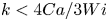$k<{4Ca}/{3Wi}$, the free surface of the viscoelastic fluid layer saturates, while for 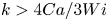$k>{4Ca}/{3Wi}$, the free surface ruptures, where $Ca$ is the capillary number.

In short, the main message is that an unbounded layer of a viscoelastic fluid under an RT configuration is conditionally stable, and when it is unstable at a critical Bond number it will bifurcate supercritically with predictable wavelengths. However, in bounded layers, the instability for viscoelastic fluids will lead to subcritical rupture of the interface for widths that are smaller than a critical value. Contrast this result with the case of RT instability of a non-elastic fluid, where the instability is always subcritical. Here the bifurcation is unconditionally unstable in an infinitely wide container and can be delayed only by narrowing the horizontal span of the container, nevertheless breaking subcritically.

An interesting extension of this work is to consider the instability of a viscoelastic fluid in a liquid bridge (Jørgensen et al. Reference Jørgensen, Le Merrer, Delanoë-Ayari and Barentin2015; Lin et al. Reference Lin, Lin, Johns and Narayanan2019) due to the similarities between the instability of a liquid bridge and RT instability (Johns & Narayanan Reference Johns and Narayanan2002). In such an extension, one might expect that, depending on the length-to-radius ratio, the liquid bridge can either saturate or rupture. This then could lead to a possible experiment that determines the surface tension and the shear modulus of a viscoelastic fluid by correlating these properties to the point of instability.