2.1 Test rig

Turbulent particle-laden pipe flows were created in a water loop driven by a centrifugal pump; see figure 1. The in-line 3 kW centrifugal pump of type DPV18-30, manufactured by ‘Duijvelaar pompen’, allowed Reynolds numbers, based on the bulk velocity, $U_{b}$ , and pipe diameter, $D$ , in the range $10^{3}$ – $10^{5}$ .

Figure 1. Schematic of the experimental 3D-PTV set-up for downward or upward particle-laden pipe flow.

A set of valves was arranged in such a way that downward and upward vertical flows were possible. A frequency controller permitted fine-tuning of the Reynolds number by adjusting the mass flow rate. The mass flow rate was measured by means of a Micro Motion Elite CMF300 mass flow (Coriolis meter) and mass density meter, whose inaccuracy was less than 0.5 % of the registered flow rate. A water reservoir (tank I) was located at the bottom of the set-up and contained approximately $2~\text{m}^{3}$ of water. This volume facilitated water temperature stabilization and Reynolds number control. The temperature during a test-run was essentially constant, varying by $0.1\,^{\circ }\text{C}$ at most. Submerged pumps were placed in the reservoir tanks at the bottom and the top (tank II, $0.15~\text{m}^{3}$ ) of the set-up in order to promote homogeneous dispersion of the added tracers and inertial particles.

The measurement section consisted of a glass pipe to ensure optical accessibility. A water-filled rectangular glass box around the pipe minimized optical distortion. The pipe inner diameter, $D=2R$ , was 100 mm and its wall thickness was 10 mm. Flow straighteners, tube bundle conditioners of ISO 5167-1:1991, see Miller (Reference Miller1996), were employed to avoid secondary flows due to bends. As a result, nearly uniform fluid velocity profiles were obtained just after the flow straighteners. In up-flow, 3D-PTV measurements were performed at $45D$ downstream of the entrance section; in down-flows, at  $20D$ .

Three ‘HighSpeedStar’ cameras with 12-bit greyscale CMOS sensors and a resolution of $1024\times 1024$  pixels were utilized to capture instantaneous 3D particle positions in a measurement volume of $10\times 10\times 10~\text{cm}^{3}$ . The cameras could record at 1000 Hz at full resolution, but were operated at 50 Hz to maximize the flow measurement time. Recordings were performed until the internal memory of the cameras became full after approximately 2 min. The maximum physically relevant frequencies were approximately 12 Hz for $Re_{b}=10\,300$ , making a 50 Hz sampling rate sufficient according to the Nyquist theorem. The lighting system comprised two stroboscopic light sources with an output of 5 J per pulse; see figure 1. The strobes were custom-built to maximize the light output at a maximum of 60 Hz with a light pulse duration of approximately  $40~\unicode[STIX]{x03BC}\text{s}$ .

2.2 Settings and accuracy of 3D-PTV

While a minimum depth of field of the camera and lenses must be guaranteed to obtain sharp images of moving particles in the whole volume of the measurement section, a certain field of view is needed to obtain trajectories long enough to measure all relevant flow scales. A focal length of 105 mm, an exposure time of $20~\unicode[STIX]{x03BC}\text{s}$ and a distance from the lens to the object of roughly 800 mm were selected. The sensor resolution was $1~\text{pixel}^{2}=17~\unicode[STIX]{x03BC}\text{m}\times 17~\unicode[STIX]{x03BC}\text{m}$ , which corresponds to an actual area of $100~\unicode[STIX]{x03BC}\text{m}\times 100~\unicode[STIX]{x03BC}\text{m}$ .

To determine the so-called calibration functions that correlate the pixel information from the three cameras to 3D world coordinates, an in situ calibration unit was designed. A calibration plate manufactured from a 2.5 mm thick glass plate with a single-sided coating of chromium, 150 nm thick, was given fixed positions at 26 locations in the pipe, interspaced by 2 mm, with a position error of less than $1~\unicode[STIX]{x03BC}\text{m}$ . Only motion perpendicular to the calibration plate was possible. A 2D array of circular gaps with a diameter of 0.3 mm covered the plate; the centres were 5 mm apart both horizontally and vertically. Third-order polynomials were found to be sufficient to connect the recorded pixel coordinates to actual positions; fitting errors were less than 0.05 pixel.

Figure 2. One out of three simultaneous recordings of particle-laden flow in the test section; frontal top camera. The inertial particles are the larger circles.

A commercial 3D-PVT imaging code from La Vision GmbH, named Davis, was used to obtain the trajectories of the tracers and inertial particles. Algorithmic details of the Davis PTV tracking code can be found in Dracos (Reference Dracos and Dracos1996) and Maas (Reference Maas and Dracos1996). Built-in imaging filters were used to improve the contrast between the tracers and the background. The 2D determination of the centre of a particle in the camera plane was made by a Gaussian fit. The so-called triangulation error is a measure of uncertainty of the 3D particle position. In the present measurements, the maximum triangulation error was 0.2 pixel, roughly $20~\unicode[STIX]{x03BC}\text{m}$ .

The particle tracking algorithm yields matrices that contain time reference and spatial positions of particle trajectories from the flow measurement images. Before the statistical analysis of turbulent pipe flow is carried out, the spatial positions are converted from Cartesian to cylindrical coordinates with radial coordinate $r$ and azimuthal coordinate $\unicode[STIX]{x1D703}$ . In the proximity of the pipe centreline, $r/R=0$ , the discontinuity of radial and tangential velocities for cylindrical coordinates can cause wrong differentiation of displacements in time. Let $\text{d}t$ be the timestep between consecutive measurements and let suffix $j$ number the time of measurement, $t_{j}$ . If a particle crosses $r=0$ , the radial velocity, $u_{r}$ , may appear to be zero, and the tangential velocity, $u_{\unicode[STIX]{x1D703}}\approx \unicode[STIX]{x03C0}r/\text{d}t$ ; see (2.1) and (2.2). This problem is avoided by employing a Cartesian frame of reference around the tube axis,

After the coordinate transformation, the differentiation in time of the validated trajectories generates the velocity vectors. In a similar way, accelerations were derived from smoothed velocity histories; see Oliveira, van der Geld & Kuerten (Reference Oliveira, van der Geld and Kuerten2015). Velocities derived by straightforward interpolations of consecutive 3D positions of a particle trajectory have been proved to be reliable to obtain pipe flow statistics. The uncertainty in the magnitude of the velocity vector obtained from two consecutive positions is for both tracers and particles approximately $0.06~\text{mm}~\text{s}^{-1}$ . Unrealistic trajectories are avoided by two filters: a length filter and an outlier check of five times the standard deviation of the velocity components. The length filter consists of elimination of particle trajectories comprising less than 10 positions. Mean and maximum particle trajectories consist of 30 and 81 positions respectively. More information about the particle tracking algorithm used to obtain the trajectories of the tracers and the inertial particles and the trajectory analysis method for individual particle trajectories is given by Oliveira (Reference Oliveira2012) and Oliveira, van der Geld & Kuerten (Reference Oliveira, van der Geld and Kuerten2013).

The number of tracer trajectories measured in the range $r/R=0.6$ –1 decreases with increasing  $r$ . The difficulties in measuring tracer trajectories in this region were mainly due to light reflections stemming from the difference between the refractive indices of water, $n\approx 1.33$ , and glass, $n\approx 1.51$ , and the curvature of the glass pipe. Light reflections deteriorate the contrast between tracers and background. However, the fluid flow could also be measured for $r/R>0.6$ despite the lower number of usable tracers there. The measured concentration of tracers is roughly linear from $r/R=0$ to 0.6 and decreases towards the wall for $r/R>0.6$ for all flow cases. In Oliveira et al. (Reference Oliveira, van der Geld and Kuerten2013), Eulerian statistics of a single-phase turbulent pipe flow acquired by 3D-PTV were found to be trustworthy in the near-wall zone if the number of velocity vectors per radial bin exceeded 1000. The same criterion is also applied in the present work.

In the detection of inertial particle trajectories, the above contrast problem between particles and background did not occur. The larger imaging projection area of inertial particles on the camera sensor, exceeding the projection of tracers by a factor of 16, avoided problems in the identification of particles; see figure 2. While the projection of a tracer image covers an area of nearly $2\times 2$  pixels, the projection of an inertial particle covers $8\times 8$  pixels. Roughly, every 3D inertial particle position identified in the tracking algorithm corresponds to a real particle. On average, approximately $3\times 10^{5}$ inertial particle positions were identified in each particle-laden case. Three-dimensional particle positions were identified with a camera frame rate of 50 Hz in average time intervals of 50 min. In this period of time, a water volume corresponding to ${\approx}2.3~\text{m}^{3}$ crosses the test section. In this way, accurate measurements of concentration profiles of inertial particles were obtained.

The derivative of particle trajectories with respect to time generates on average $2\times 10^{6}$ velocity vectors for tracers and $3\times 10^{5}$ for inertial particles in each particle-laden case. The velocity vectors are ensemble-averaged in radial bands with a width of $\unicode[STIX]{x0394}r=1$  mm, except for the first bin, which extends from $r=0$ to $r=0.5$  mm; see Oliveira et al. (Reference Oliveira, van der Geld and Kuerten2013). A cylindrical coordinate system $(r,\unicode[STIX]{x1D703},z)$ with origin at the pipe centreline and with the axial axis, $z$ , anti-parallel to the gravitational acceleration, $\boldsymbol{g}$ , is used for both down- and up-flow.

To check the accuracy of the mean axial velocity profiles, the products of the mean axial fluid velocity and the area of each discrete bin, $\langle U_{z}\rangle _{k}\,A_{k}$ , were summed to obtain the mean volumetric flow rate, $Q$ , through the measurement volume. Temperature measurements yielded the water mass density, $\unicode[STIX]{x1D70C}$ . The resulting product $\unicode[STIX]{x1D70C}Q$ corresponded to the mass flow rate given by the Coriolis meter within its accuracy range.

2.3 Properties of particles

The properties of the polystyrene particles applied in the present particle-laden experiments are given in table 1. The fluid time scale $\unicode[STIX]{x1D70F}_{\unicode[STIX]{x1D702}}$ at the Stokes number $St$ and the fluid length scale $\unicode[STIX]{x1D702}$ are the Kolmogorov scales for fully developed single-phase pipe flow at $Re_{b}=10\,300$ , as computed from DNS results by Veenman (Reference Veenman2004). The Kolmogorov length varies between 0.6 mm in the pipe core and 0.2 mm at the wall, whereas the Kolmogorov time varies between 187 ms in the core and 57 ms at the wall. The Reynolds number based on the wall shear velocity and the pipe diameter, $Re_{\unicode[STIX]{x1D70F}}$ , is 647. For evaluation of the particle time scale, $\unicode[STIX]{x1D70F}_{p}$ , the relaxation time for particles in stationary flow is used; see Albrecht et al. (Reference Albrecht, Borys, Damaschke and Tropea2003):

where $\unicode[STIX]{x1D707}$ is the dynamic viscosity of the fluid, $d_{p}$ is the particle diameter and $\unicode[STIX]{x1D70C}_{p}$ and $\unicode[STIX]{x1D70C}_{f}$ are the mass densities of the particles and the fluid respectively. A relaxation time of $\unicode[STIX]{x1D70F}_{p}\approx 4$  ms is obtained for the tracers. It should be noted that the fluid inertia is accounted for by the added mass coefficient 0.5, which close to a wall is increased to approximately 0.7; see van der Geld (Reference van der Geld2002).

The terminal velocity specified in table 1 is attained in quiescent fluid when the gravitational and drag forces are in equilibrium,

where $g$ is the gravitational acceleration and $C_{D}$ is the drag coefficient; it should be noted that $U_{TV}$ is positive by definition. The drag coefficient is a function of the particle Reynolds number, $Re_{p}=d_{p}U_{TV}/\unicode[STIX]{x1D708}$ , which is based on the particle diameter and the terminal velocity. In the Stokes regime, $C_{D}$ is given by (2.5). For $1<Re_{p}<1000$ , Schiller & Naumann (Reference Schiller and Naumann1935) proposed the correlation given by (2.6),

The properties of the inertial particles are such that the characteristic root-mean-square velocity representative of the turbulent carrier phase, $u_{rms}$ , and the terminal velocity of the dispersed phase, $U_{TV}$ , are approximately the same, $u_{rms}/U_{TV}=O(1)$ .

Since the bulk flow velocity, $U_{b}$ , is approximately $100~\text{mm}~\text{s}^{-1}$ , the ratio $U_{b}/U_{TV}$ is of the order of $10^{2}$ for seeding particles; see table 1. Since $U_{b}\gg U_{TV}$ , $\unicode[STIX]{x1D70F}_{p}<\unicode[STIX]{x1D70F}_{\unicode[STIX]{x1D702}}$ and $d_{p}<\unicode[STIX]{x1D702}$ , the seeding particles employed work well as flow tracers. For the inertial particles, the ratio $U_{b}/U_{TV}$ is of the order of 10, $\unicode[STIX]{x1D70F}_{p}\approx \unicode[STIX]{x1D70F}_{f}$ and $d_{p}>\unicode[STIX]{x1D702}$ . Therefore, the inertial particles have significant inertial characteristics, as is also exhibited by the differences in the Lagrangian statistical properties, the auto- and cross-correlations of velocities and the accelerations of tracers and inertial particles; see Oliveira et al. (Reference Oliveira, van der Geld and Kuerten2015). These authors showed that the decay of the Lagrangian velocity correlations of the applied inertial particles takes place in shorter times than the decay of the velocity correlation of the flow tracers. The fluctuating velocity of a particle is coherent with the fluid as long as it remains in a characteristic large eddy structure. However, the inertial particles applied here cannot completely follow the large fluid scales due to their inertia (mainly from their finite size) and the acceleration of the fluid volume, which is named added mass. One of the reasons for the difference in tracer and particle behaviour is the so-called crossing trajectory effect, where a particle heavier than the surrounding fluid falls in an external force field, such as gravity, from one eddy to another at a rate faster than the average eddy decay rate. In addition, particles of intermediate size in shear flows experience a hydrodynamic lift.

2.4 Experimental conditions

Downward and upward vertical flows were measured at the same bulk Reynolds number based on the tube diameter, $Re_{b}$ . The bulk velocity of each flow, $U_{b}$ , was adapted to temperature changes to keep $Re_{b}\approx 10\,300$ . Single-phase flows served as a reference for two-phase flows. Only tracers were employed in single-phase flow measurements. Both tracers and inertial particles were present in particle-laden measurements. A mean volume fraction of tracers of less than $10^{-6}$ was applied to all experiments to prevent the enhancement of dissipation effects; see Elghobashi (Reference Elghobashi1994). Particle-laden flows with a mean volume fraction of inertial particles, $\langle \unicode[STIX]{x1D6F7}_{v}\rangle$ , ranging from $5.0\times 10^{-6}$ to $3.2\times 10^{-5}$ were tested.

A particle-laden experimental case is represented here by a number indicating the flow direction (1 or 2) and a letter indicating the mean concentration of inertial particles (A, B or C); see table 2. The reference single-phase flows are 1S and 2S. Details on the single-phase pipe flow based on the scales of the current experiment and in fully developed conditions (case 1S) are presented in table 3. The variables $Re_{b}$ , $Re_{\unicode[STIX]{x1D70F}}$ , $U_{b}$ , $\unicode[STIX]{x1D702}$ and $\unicode[STIX]{x1D70F}_{\unicode[STIX]{x1D702}}$ have already been defined above; $U_{c}$ is the centreline velocity and $\unicode[STIX]{x1D708}$ is the fluid kinematic viscosity. The wall shear velocity, $u_{\unicode[STIX]{x1D70F}}$ , was derived from DNS data provided by Veenman (Reference Veenman2004) by implementing the actual pipe diameter. In the remainder of this work, the bulk velocity $U_{b}$ is chosen as a normalization quantity instead of the wall shear velocity, $u_{\unicode[STIX]{x1D70F}}$ , which is often used in the literature, because $U_{b}$ can be determined more accurately in our experimental set-up; see § 2.2. The single-phase flow experimental results of Oliveira et al. (Reference Oliveira, van der Geld and Kuerten2013) at $Re_{b}=10\,300$ were in accordance with the DNS results. The significance of the pipe flow in relation to the particle motion can be inferred by comparing tables 1 and 3, and by the graphical results in § 3. The maximum root-mean-square fluid velocity occurs at $r/R\sim 0.95$ and for the streamwise direction.

2.5 Point-particle DNS

This paper is focused on experimental findings and the interpretation thereof. However, in order to be able to interpret some of the results, we also performed numerical simulations of particle-laden turbulent pipe flow at the same Reynolds number for up-flow. These simulations are not intended to cover the complete physics of the problem, but to complete the understanding of the experimental findings.

In a real DNS, all scales of the flow around each particle should be resolved, which is computationally unfeasible with many particles. Usually, PP-DNS is performed in cases where the number of particles or the range of scales is too large, although PP-DNS is often assumed to be only valid in cases where the particles are small compared with the Kolmogorov scale (Bagchi & Balachandar Reference Bagchi and Balachandar2003; Balachandar & Eaton Reference Balachandar and Eaton2010; Vreman Reference Vreman2016), which is certainly not true in our experiments. However, since the particle volume fraction in our experiments is so small that the effects of the particles on the continuous phase are negligible, one-way coupled PP-DNS and a force balance on each particle that includes all relevant forces exerted by the fluid on the particles will be used here. One of the advantages of the one-way coupling is that the liquid velocity and liquid vorticity at the centre of the particle, needed for some of the forces on the particle, are well-defined.

The present section briefly describes the numerical method of the PP-DNS. An Eulerian–Lagrangian approach is applied, where the continuous phase is described in an Eulerian way by the incompressible Navier–Stokes equations in cylindrical coordinates and each particle is tracked in a Lagrangian way by solving its equation of motion. The numerical method for the continuous phase is the same as in Walpot, van der Geld & Kuerten (Reference Walpot, van der Geld and Kuerten2007). A pipe with a length equal to $5D$ is used together with periodic conditions in the axial direction. Naturally, the boundary conditions in the tangential direction are periodic as well. A Fourier–Galerkin method is applied in the two periodic directions, and in the radial direction a Chebyshev collocation method is applied, but the radial direction is divided into several elements with a Chebyshev distribution of grid points in each of them to avoid excessive clustering of grid points near the axis of the pipe. The nonlinear terms in the Navier–Stokes equation are calculated in Fourier space making use of the $3/2$ rule to avoid aliasing. For the present bulk Reynolds number of 10 300, the numbers of grid points are 150 in the radial direction, 256 in the tangential direction and 384 in the axial direction. It has been shown by Oliveira et al. (Reference Oliveira, van der Geld and Kuerten2013) that this resolution is sufficient to obtain good agreement with experimental results for single-phase flow. Time integration is performed with a second-order-accurate time-splitting method, in which the nonlinear terms are treated explicitly and the viscous and pressure terms implicitly.

At the low particle–fluid mass density ratio considered here, all forces exerted by the fluid on a particle need to be taken into account, but for computational reasons we omit the Basset history force. Therefore, the equation of motion on each particle comprises the buoyancy force, the pressure gradient force, the added mass force, the drag force and the shear lift force,

The vorticity of the flow field, $\unicode[STIX]{x1D735}\times \boldsymbol{U}$ , is denoted by $\unicode[STIX]{x1D74E}$ , and $\text{D}\boldsymbol{U}/\text{D}t$ represents the Lagrangian fluid acceleration, which is the sum of the pressure gradient acceleration and a viscous deceleration,

The undisturbed fluid velocity, $\boldsymbol{U}(\boldsymbol{x}_{\boldsymbol{p}})$ , is by definition at the location of the centre of mass of the particle, $\boldsymbol{x}_{\boldsymbol{p}}$ . The coefficients $C_{AM}$ , $C_{D}$ and $C_{L}$ denote the added mass, drag and lift coefficients respectively. The coefficient $C_{AM}$ is taken to be 0.5, $C_{D}$ is computed with the Schiller & Naumann (Reference Schiller and Naumann1935) correlation given by (2.5) and (2.6), and $C_{L}$ is given by the following correlation, valid for low Reynolds numbers $Re_{s}=d_{p}^{2}|\unicode[STIX]{x1D74E}|\unicode[STIX]{x1D70C}_{f}/\unicode[STIX]{x1D707}$ (van der Geld Reference van der Geld1997):

In order to obtain the fluid velocity, vorticity and acceleration at the particle position, tri-linear interpolation is applied. Stability problems near the pipe axis are prevented by using the equations for the Cartesian components of particle position and velocity. Moreover, for the particles, periodic conditions are applied in the axial direction. Particles collide elastically with the wall of the pipe. The number of particles tracked in the simulation is larger than in the experiments. Since only one-way coupling is applied, this does not change the results but does increase the statistical accuracy of the results.

The simulation is started from a fully developed turbulent flow to which particles are added at random positions, uniformly distributed over the whole volume of the pipe. The initial velocity of a particle is equal to the velocity of the fluid at the position of the particle. Statistical results for the particle properties are gathered after a statistically steady particle volume fraction distribution in the radial direction has been reached. Simulations are only performed for up-flow. For down-flow, the lift force leads to a strong motion of particles towards the wall of the pipe, resulting in a locally high particle concentration, so that two-way coupling and particle collisions cannot be disregarded.

3.1 Assessment of the extent of flow development

Especially for the experiments in down-flow, the distance between the flow straightener and the measurement section might be too small to obtain fully developed flow in the measurement section. Therefore, we will first investigate to what extent the velocity statistics obtained for single-phase flow correspond to fully developed results obtained by means of DNS (Veenman Reference Veenman2004; Walpot et al. Reference Walpot, van der Geld and Kuerten2007) at the same Reynolds number. The diagonal components of the Reynolds stress tensor of the single-phase results for up-flow will be seen to correspond well with the DNS results, which indicates that this flow is indeed fully developed; see also Oliveira et al. (Reference Oliveira, van der Geld and Kuerten2013). However, deviations of up to 15 % will be seen to occur in the results for down-flow, which can only be explained by a too small distance between the flow straightener and the measurement section, which equals $20D$ . The deviations are restricted to the regions close to their maxima, i.e. $0.6<r/R<0.9$ . Moreover, the mean axial velocity profiles differ by only 2 % at most. Although a well-known correlation predicts that the entrance length equals approximately $20D$ in the present experiment (Hinze Reference Hinze1975), this distance is apparently insufficient for a fully developed flow in all respects. Nevertheless, the magnitude and extent of the deviations of the experimental single-phase down-flow results from fully developed flow (DNS or up-flow) are sufficiently small to discriminate important trends in the behaviour of inertial particles, as will be shown in this paper. In addition, the results of the present research can be applied to validate DNS results on particle-laden flow.

It should be noted that the development length of two-phase flow is generally larger than that of single-phase flow. Therefore, the observation that the single-phase up-flow is fully developed does not imply that the particle concentration in the corresponding two-phase flow is fully developed in the measurement section. This will be investigated in the next section.

3.2 Volume fraction profiles of inertial particles

In this section, we will first investigate the particle volume fraction profiles for both up-flow and down-flow and then give an explanation for the observed behaviour by considering the particle equation of motion. Figure 3 shows the particle volume fraction as a function of the radial coordinate for up-flow and down-flow and for all mean particle volume fractions studied. The error bars have a size of $\pm 2$ times the standard error. A sample corresponds to the instantaneous volume fraction found in one measurement for a given radial position, and the mean volume fraction corresponds to the time-averaged volume fraction of particles at this same location.

Figure 3. Volume fraction profiles of inertial particles, $\unicode[STIX]{x1D719}_{v}(r/R)$ , for various values of the mean particle volume fraction. (a) Up-flow; (b) down-flow.

The results presented in figure 3 are consistent: the volume fraction profiles are hardly affected even when half of the total number of samples is used. Figure 3(a) shows that in up-flow, the particle volume fraction is smaller close to the pipe wall, i.e. for $r/R>0.85$ , than in the centre. For down-flow, on the other hand, a distinct large peak at $r/R\approx 0.97$ is observed. This shows that the volume fraction profile strongly depends on the direction of the flow, in particular in the near-wall zone. The results for down-flow also show a second peak at $r/R=0$ but with a significantly smaller magnitude than the peak near the wall. This central peak finds its origin in the development of the flow. Just after the flow straightener on top, the velocity profile is close to being uniform. Subsequent development of the flow requires motion towards the centre. This flow carries particles along. Further downstream, this peak will disappear. It should be noted that turbophoresis, particle motion towards the wall of a pipe by the effect of turbulence, cannot explain the concentration results. If this effect was dominant, the concentration profiles in up- and down-flows should be similar.

The observed differences in particle volume fraction profiles between up-flow and down-flow can be explained by the forces exerted on the particles. If the three main forces of the particle equation of motion are retained, equation (2.7) reduces to

The main contribution from the vorticity to this equation is through the contribution to its tangential component from the mean axial velocity $\text{d}\langle U_{z}\rangle /\text{d}r$ close to the wall. The axial component of (3.1) therefore results in $v_{p,z}=U_{z}-U_{TV}$ . The radial component provides a balance between lift and drag and can be simplified to $v_{p,r}=4d_{p}(C_{L}/C_{D})\text{d}\langle U_{z}\rangle /\text{d}r/3$ . For up-flow, this radial particle velocity is directed towards the centre of the pipe, whereas for down-flow, it is directed towards the wall. Point-particle DNS simulations without lift force resulted in uniform particle concentrations, which confirms the above explanation. Next, we will use force balance (3.1) to estimate the magnitude of the mean radial particle velocity.

If only the dominant forces are retained, the radial component of (3.1) can be written as

Let $\text{sgn}(\langle U_{z}\rangle )$ denote the sign of the mean axial velocity component. As will be shown below, the mean value of $|\boldsymbol{v}_{p}-\langle \boldsymbol{U}\rangle _{L}|$ is close to $U_{TV}$ . We use the notation $\langle \;\rangle _{L}$ to indicate a Lagrangian average, i.e. the average value taken over all particles located at a certain radial coordinate. Now, suppose that an inertial particle is moving towards the centre of the tube. The drift velocity of the inertial particles in the radial direction can be defined as the value of $\langle v_{rel,r}\rangle _{L}$ that follows from (3.2),

If the lift force coefficient is taken to be 0.5 and the mean value of $\text{d}\langle U_{z}\rangle /\text{d}r$ for $0<r/R<0.6$ is employed, a drift velocity of $0.1~\text{mm}~\text{s}^{-1}$ is found, directed towards the wall for down-flow and towards the centre of the pipe for up-flow. The measured mean radial particle velocity is indeed of the order of $U_{drift}$ for $0<r/R<0.6$ , while for $0.8<r/R<1.0$ , it is systematically negative in up-flow and positive in down-flow, with absolute maxima of approximately $0.6~\text{mm}~\text{s}^{-1}$ in both cases.

Figure 4. Mean axial velocity profiles, $\langle U_{z}\rangle$ and $\langle v_{p,z}\rangle$ , of the particle-laden case 1B and the single-phase flow 1S (up-flow), (a) in the range $0<r/R<0.85$ and (b) in the range $0.85<r/R<1$ . The velocities are normalized by the bulk velocity of each flow, $U_{b}$ . The lines are added to guide the eye. The difference in scales should be noted.

Figure 5. Mean axial velocity profiles, $\langle U_{z}\rangle$ and $\langle v_{p,z}\rangle$ , of the particle-laden case 2B and the single-phase flow 2S (down-flow), (a) in the range $0<r/R<0.8$ and (b) in the range $0.8<r/R<1$ . The velocities are normalized by the bulk velocity of each flow, $U_{b}$ . The lines are added to guide the eye. The difference in scales should be noted.

Upstream of the measurement section, just behind the flow straightener, the inertial particles are still homogeneously distributed over the cross-section of the pipe and no preferential concentration is present yet. At this position, the mean radial fluid velocity evaluated at the particle positions is still equal to the Eulerian mean radial fluid velocity, which is equal to zero. As a result of (3.3), the mean radial particle velocity is directed towards the axis of the pipe for up-flow and towards the pipe wall for down-flow. The measured non-zero radial particle velocity shows that the particle concentration is not yet fully developed in the measurement section.

3.3 Mean axial velocity profiles

Figures 4 and 5 show the mean axial velocity profiles of the fluid, $\langle U_{z}\rangle$ , and the inertial particles, $\langle v_{p,z}\rangle$ , for up- and down-flow. All velocities in this paper are normalized with the bulk fluid velocity, $U_{b}$ , which varies from case to case. The bulk flow velocity was adjusted to keep the bulk Reynolds number for each experiment equal to 10 300. The error bars have sizes comparable to the dimensions of the symbols and are not shown.

The mean axial fluid velocity in two-phase up-flow is slightly smaller than the corresponding single-phase velocity in most of the cross-section of the pipe. This is caused by the particles, which have a smaller velocity, dragging the fluid along. The opposite is observed in figure 5 for down-flow. It should be noted that the cross-sectional average fluid velocity is the same in all cases. Therefore, this small difference in axial velocities is compensated close to the wall (figures 4 b and 5 b).

The relative velocity is approximately constant in the range $0<r/R<0.5$ . This difference is approximately equal to $10.2~\text{mm}~\text{s}^{-1}$ , which is the value of $U_{TV}$ ; see table 1. The difference decreases further away from the pipe axis. For $r/R>0.90$ , the mean fluid and particle velocities are almost equal; see figure 6, where the difference between the relative velocity and the terminal velocity, $U_{TV}$ , is shown as a function of the radial coordinate. Understanding of this finding is facilitated by a study of the PP-DNS results for the same flow. Figure 7 shows various mean axial velocity profiles obtained in the PP-DNS for up-flow. 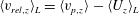The mean fluid velocity, $\langle U_{z}\rangle$ , the mean particle velocity, $\langle v_{p,z}\rangle$ , the mean fluid velocity at the particle positions, $\langle U_{z}\rangle _{L}$ , and the absolute value of the mean relative velocity, which is defined as $\langle v_{rel,z}\rangle _{L}=\langle v_{p,z}\rangle -\langle U_{z}\rangle _{L}$ , are included (mean is here defined as the average over time and the two homogeneous directions). It should be noted that this relative velocity is not accessible in measurements, since it requires the fluid velocity at the particle position, which is not defined. In particle-resolved DNS, this quantity is not defined either, but for this reason we applied PP-DNS.

Figure 6. The difference between the mean axial particle and fluid velocities, $\langle v_{rel,z}\rangle$ , for up-flow (a) and down-flow (b).

Figure 7 shows that if $r/R<0.7$ , the difference between $\langle U_{z}\rangle$ and $\langle U_{z}\rangle _{L}$ is negligible, which implies that the mean relative velocity as seen by the particle is equal to $U_{TV}$ . Closer to the wall, the Lagrangian averaged axial fluid velocity starts to deviate from its Eulerian averaged value. Apparently, particles are preferentially located in regions where the axial fluid velocity component has a higher absolute value than the mean fluid velocity. This can be understood in the following way. Consider an inertial particle in developed upward pipe flow outside the core of the pipe. It is driven there by a positive radial fluid velocity fluctuation. Since the Reynolds stress of the fluid is positive, the axial fluid velocity fluctuation must also be positive on average. The instantaneous axial velocity of the particle, $v_{pz}$ , is the sum of the constant $-U_{TV}$ and the fluid velocity, as shown by the PP-DNS results of figure 7. The value of $v_{pz}$ is therefore preferentially shifted to positive values of fluid velocity fluctuations. The lower Eulerian mean relative velocity near the wall also results from this.

Figure 7. Point-particle DNS computations of local mean axial velocity components. The dashed line gives the component of the inertial particles and the dotted line the mean liquid velocity at the particle position. The mean fluid velocity (solid) and the absolute value of the local mean relative velocity as sampled by the particles, $|\langle v_{rel,z}\rangle _{L}|$ (symbols), are also given.

A similar finding to that in figure 6(b) for the range $r/R<0.6$ , where $-U_{TV}\approx \langle v_{rel,z}\rangle$ , was observed by Suzuki et al. (Reference Suzuki, Ikenoya and Kasagi2000) in downward channel flow of water with ceramic beads with mass density exceeding the carrier phase by a factor of 3.85. The ratios of the root-mean-square (RMS) fluid velocity to the terminal velocity of the inertial particles, $u_{rms}/U_{TV}$ , in their experiments are close to 0.2, which is different from the value of approximately 1 in the present study. A maximum concentration of inertial particles occurred near the channel walls, similarly to the down-flow measurements presented here, and $|\langle v_{rel,z}\rangle |$ was also found to decrease with decreasing distance from the wall. Suzuki et al. (Reference Suzuki, Ikenoya and Kasagi2000) observed that the velocity difference between the carrier phase and the inertial particles is approximately equal to the terminal velocity. Near the wall, they observed a reduction of the relative velocity of approximately 10 % of  $U_{TV}$ .

In the next section, it will be shown that the above explanation of the relative velocity is consistent with the interpretation of the particle Reynolds stress tensor.

3.4 Reynolds stress tensors of the fluid and the dispersed phase

In this section, the components of the Reynolds stress tensor, $\unicode[STIX]{x1D619}_{ij}$ , which are averages of the products of velocity fluctuations, with $i$ and $j$ denoting cylindrical coordinates ( $r$ , $\unicode[STIX]{x1D703}$ , $z$ ), are assessed for both phases. We use $\unicode[STIX]{x1D619}_{ij}^{\,f}=\langle u_{i}u_{j}\rangle$ for the fluid phase and $\unicode[STIX]{x1D619}_{ij}^{p}=\langle v_{pi}^{\prime }v_{pj}^{\prime }\rangle$ for the dispersed phase. In fully developed pipe flow, the only decoupled direction is the tangential one, which implies that all cross-correlations involving the tangential velocity are zero, which is confirmed by the experimental results.

Figure 8. Radial and tangential components of the Reynolds stress tensor, $\unicode[STIX]{x1D619}_{rr}^{\,f}$ , $\unicode[STIX]{x1D619}_{rr}^{p}$ , $\unicode[STIX]{x1D619}_{\unicode[STIX]{x1D703}\unicode[STIX]{x1D703}}^{\,f}$ and $\unicode[STIX]{x1D619}_{\unicode[STIX]{x1D703}\unicode[STIX]{x1D703}}^{p}$ , for upward cases 1B/1S (a) and downward cases 2B/2S (b). The results are normalized by the square of the bulk velocity of each flow, $U_{b}^{2}$ . The lines are added to guide the eye.

Figure 9. Axial components of the Reynolds stress tensor, $\unicode[STIX]{x1D619}_{zz}^{\,f}$ and $\unicode[STIX]{x1D619}_{zz}^{p}$ , for upward cases 1B/1S (a) and downward cases 2B/2S (b). The results are normalized by the square of the bulk velocity of each flow, $U_{b}^{2}$ . The lines are added to guide the eye.

The non-zero components of the Reynolds stress tensor are presented in figures8–10. All results are normalized by the square of the bulk flow velocity of the corresponding experiment. In each plot, the single-phase results are also shown.

In Oliveira et al. (Reference Oliveira, van der Geld and Kuerten2013), the non-zero components of the Reynolds stress tensor of the fluid of case 1S were shown to agree with the DNS results of Veenman (Reference Veenman2004). While at the centre of the tube ( $r/R<0.2$ ) turbulence is nearly homogeneous, highly inhomogeneous behaviour is seen closer to the wall ( $0.8<r/R<1$ ); see figures 8 and 9.

Figures 8–10 show that the results for the tracers in particle-laden flow are almost indistinguishable from the single-phase flow results. This shows that the particle concentration in the experiments is so low that the particles do not significantly affect the carrier phase. Therefore, the modification of flow turbulence is not of concern in the present study due to the low concentration of particles applied. The noisy character of the symbols for the Reynolds stresses of the inertial particles in figures 8–10 can be attributed to the number of velocity samples: $2\times 10^{6}$ velocity vectors for tracers and only $3\times 10^{5}$ for inertial particles in each particle-laden case; see § 2.2.

Figure 10. Non-diagonal components of the Reynolds stress tensor, $\unicode[STIX]{x1D619}_{rz}^{\,f}$ and $\unicode[STIX]{x1D619}_{rz}^{p}$ , for upward cases 1B/1S (a) and downward cases 2B/2S (b). The results are normalized by the square of the bulk velocity of each flow, $U_{b}^{2}$ . The lines are added to guide the eye.

The radial and tangential diagonal components of the Reynolds stress tensor of the dispersed phase are almost equal to the corresponding results for the carrier phase for both up-flow (figure 8 a) and down-flow (figure 8 b). However, the diagonal axial and non-zero non-diagonal components of the Reynolds stress tensor of the fluid and the dispersed phase are not equal. In the range $r/R<0.8$ , $\unicode[STIX]{x1D619}_{zz}^{p}$ exceeds $\unicode[STIX]{x1D619}_{zz}^{\,f}$ by more than 20 % for up-flow (figure 9 a) and by more than 15 % for down-flow (figure 9 b). For $r/R>0.8$ in up-flow, both $\unicode[STIX]{x1D619}_{rz}$ and $\unicode[STIX]{x1D619}_{zz}$ for the particles are significantly smaller than for the fluid.

In order to explain this observed behaviour of the Reynolds stress tensor of the dispersed phase for $r/R>0.8$ , we invoke the concept of turbulent diffusion. Turbulent diffusion theory establishes a relation between the non-diagonal component of the Reynolds stress tensor and the radial derivative of the axial fluid velocity of the form

The closure (3.4) is only approximate but offers a convenient way to qualitatively understand the phenomenon of turbulent diffusion. Since $\text{d}\langle U_{z}\rangle /\text{d}r<0$ in pipe flow, this relation shows that $\unicode[STIX]{x1D619}_{rz}^{\,f}>0$ . Next, we turn to the particle Reynolds stress. Due to the direction of the lift force from the wall to the centre of the pipe, particles near the wall in up-flow are mainly driven by sweeps from the centre to the wall. For $r/R>0.7$ , these particles are therefore in eddies that carry a lower absolute value of the velocity gradient $\text{d}\langle U_{z}\rangle /\text{d}r$ . This is why the Lagrangian sampled average of this gradient, $|\langle \text{d}U_{z}/\text{d}r\rangle _{L}|$ , is smaller than the Eulerian average. The results of the PP-DNS, shown in figure 11(a), confirm this.

Figure 11. Comparison of $\langle \unicode[STIX]{x2202}U_{z}/\unicode[STIX]{x2202}r\rangle _{L}$ and $\unicode[STIX]{x2202}\langle U_{z}\rangle /\unicode[STIX]{x2202}r$ , made dimensionless with the tube radius ( $R$ ) and bulk velocity ( $U_{b}$ ), as computed by PP-DNS (a); probability density, $P$ , of $(\unicode[STIX]{x2202}U_{z}/\unicode[STIX]{x2202}r)R/U_{b}$  (b).

The probability density function (p.d.f.) of the Lagrangian sampled $\unicode[STIX]{x2202}U_{z}/\unicode[STIX]{x2202}r$ at $r/R=0.9$ , shown in figure 11(b), is a further illustration of this. This figure also shows the Eulerian average (approximately $-2U_{b}/R$ , indicated by the vertical line). Diffusion theory for both the fluid and particle Reynolds stresses (3.4) now explains why $R_{rz}^{p}<R_{rz}^{\,f}$ close to the wall.

At the same time, the Reynolds stress $R_{zz}$ of inertial particles outside the core of the pipe is less than for fluid particles (figure 9 a). This is substantiated by the PP-DNS results, which indeed showed that $\langle U_{z}\rangle _{L}$ exceeds the Eulerian counterpart $\langle U_{z}\rangle$ (figure 7), while the Reynolds particle stresses are close to the experimental values; see figure 12.

Figure 12. Reynolds stress tensor components measured in up-flow (symbols) and computed for the particles with the point-force model in PP-DNS (solid line).

In contrast to up-flow, in down-flow and close to the wall, particles are not mainly driven by sweeps from the wall to the centre, since other mechanisms force particles away from the wall. Because of the large local particle concentration, diffusion is stronger near the wall than in the core. In addition, an inertial particle must also bounce at the wall. The Lagrangian average of $\text{d}U_{z}/\text{d}r$ is therefore about the same as the Eulerian average. As a consequence, the Reynolds stresses $\unicode[STIX]{x1D619}_{rz}^{p}$ and $\unicode[STIX]{x1D619}_{zz}^{p}$ of inertial particles are close to the corresponding fluid Reynolds stresses.

For $r/R<0.8$ , the particle Reynolds stresses are 15 % larger (figures 9 b and 10 b). The reason for this is probably that the down-flow case is not fully developed. This has been verified by the observation that upon removing the flow straightener at the inlet, as presented in Oliveira (Reference Oliveira2012), the turbulent stresses become higher.