2.1 Scheme design

In this algorithm, four steps are adopted: target tracking with multiple models, target smoothing, model probability estimation and feature extraction of target models. Finally, target features such as target motion model conversion frequency are extracted to distinguish light and small UAV targets from flying birds. The algorithm flow chart is shown in Fig. 1. Existing target tracking methods estimate target state information by establishing target motion model and modify target state by using measurement information, whose purpose is to improve tracking accuracy and approximate the real moving state of target. The goal of this method is not to improve the tracking accuracy but to realise the recognition and classification of the target, which is an extension application of the existing target tracking algorithm.

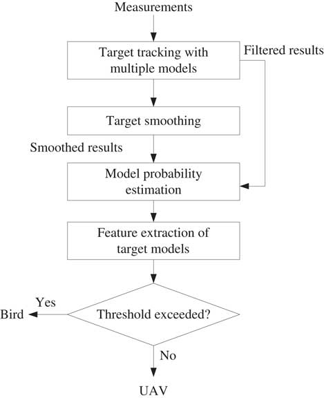
Figure 1 Classification scheme for unmanned aerial vehicle (UAV) and flying bird targets.

2.2 Target tracking with multiple models

In each time step, the initial conditions are obtained for certain model-matched filter by mixing the state estimates produced by all filters from the previous time step under the assumption that this particular model is the right model at current time step. Then standard Kalman filtering is performed for each model, and after that we compute a weighted combination of updated state estimates produced by all the filters yielding a final estimate for the state and covariance of the Gaussian density in that particular time step. The weights are chosen according to the probabilities of the models, which are computed in filtering step of the algorithm.

The mixing probabilities $$\rmu _{k}^{{i\,\mid\,j}} $$ for each model M ⁱ and M ^j are calculated as

(1) $$\bar{c}_{j} {\equals}\mathop{\sum}\limits_{i{\equals}1}^n {p_{{ij}} \rmu _{{k{\minus}1}}^{i} } ,$$

(2) $$\rmu _{k}^{{i\,\mid\,j}} {\equals}{1 \over {\bar{c}_{j} }}p_{{ij}} \rmu _{{k{\minus}1}}^{i} ,$$

where $$\rmu _{{k{\minus}1}}^{i} $$ is the probability of model M ⁱ in the time step k−1 and $$\bar{c}_{j} $$ a normalisation factor.

Now we can compute the mixed mean and covariance for each filter as

(3) $${\bf m}_{{k{\minus}1}}^{{0j}} {\equals}\mathop{\sum}\limits_{i{\equals}1}^n {\rmu _{k}^{{i\,\mid\,j}} {\bf m}_{{k{\minus}1}}^{i} } ,$$

(4) $${\bf P}_{{k{\minus}1}}^{{0j}} {\equals}\mathop{\sum}\limits_{i{\equals}1}^n {\rmu _{k}^{{i\,\mid\,j}} {\times}\left\{ {{\bf P}_{{k{\minus}1}}^{i} {\plus}\left[ {{\bf m}_{{k{\minus}1}}^{i} {\minus}{\bf m}_{{k{\minus}1}}^{{0j}} } \right]\left[ {{\bf m}_{{k{\minus}1}}^{i} {\minus}{\bf m}_{{k{\minus}1}}^{{0j}} } \right]^{T} } \right\}} ,$$

where $${\bf m}_{{k{\minus}1}}^{i} $$ and $${\bf P}_{{k{\minus}1}}^{i} $$ are the updated mean and the covariance for model i at time step k−1.

In the filtering step, for each model M ⁱ , the filtering is done as

(5) $$\left[ {{\bf m}_{k}^{{{\minus},i}} ,{\bf P}_{k}^{{{\minus},i}} } \right]{\equals}{\rm KF}_{{\rm p}} ({\bf m}_{{k{\minus}1}}^{{0j}} ,{\bf P}_{{k{\minus}1}}^{{0j}} ,{\bf A}_{{k{\minus}1}}^{i} ,{\bf Q}_{{k{\minus}1}}^{i} ),$$

(6) $$\left[ {{\bf m}_{k}^{i} ,{\bf P}_{k}^{i} } \right]{\equals}{\rm KF}_{{\rm u}} ({\bf m}_{k}^{{{\minus},i}} ,{\bf P}_{k}^{{{\minus},i}} ,{\bf y}_{k} ,{\bf H}_{k}^{i} ,{\bf R}_{k}^{i} ),$$

where the prediction and update steps of the standard Kalman filter are denoted with KF_p(⋅) and KF_u(⋅), correspondingly. In addition to mean and covariance, the likelihood of the measurement is also computed for each filter as

(7) $${\bf \Lambda }_{k}^{i} {\equals}N({\bf v}_{k}^{i};\,0,{\bf S}_{k}^{i} ),$$

where $${\bf v}_{k}^{i} $$ is the measurement residual and $${\bf S}_{k}^{i} $$ is covariance for model M ⁱ in the KF update step.

The probabilities of each model M ⁱ at time step k are calculated as

(8) $$c{\equals}\mathop{\sum}\limits_{i{\equals}1}^n {\Lambda _{k}^{i} \bar{c}_{i} } ,$$

(9) $$\rmu _{k}^{i} {\equals}{1 \over c}\Lambda _{k}^{i} \bar{c}_{i} ,$$

where c is a normalising factor.

Finally, the combined estimate for the state mean and covariance are computed as

(10) $${\bf m}_{k} {\equals}\mathop{\sum}\limits_{i{\equals}1}^n {\rmu _{k}^{i} {\bf m}_{k}^{i} } $$

(11) $${\bf P}_{k} {\equals}\mathop{\sum}\limits_{i{\equals}1}^n {\rmu _{k}^{i} {\times}\left\{ {{\bf P}_{k}^{i} {\plus}[{\bf m}_{k}^{i} {\minus}{\bf m}_{k} ][{\bf m}_{k}^{i} {\minus}{\bf m}_{k} ]^{T} } \right\}} $$

2.3 Target smoothing

It is useful to smooth the state estimates by using all the obtained measurements. Since the optimal fixed-interval smoothing with n models and N measurements requires running n ^N smoothers, we must resort to suboptimal approaches. One possibility is to combine the estimates of two filters, one running forwards and the other backwards in time. This approach is restricted to systems having invertible state dynamics, which is always the case for discretised continuous-time systems.

First we shall review the equations for the filter running backwards in time and then the actual smoothing equations combining the estimates of the two filters.

Our aim is now to compute the backward filtering density p( x _k | y _k:N ) for each time step, which is expressed as a sum of model conditioned densities

(12) $$p({\bf x}_{k} \,\mid\,{\bf y}_{{k\,\colon\,N}} ){\equals}\mathop{\sum}\limits_{j{\equals}1}^n {\rmu _{k}^{{b,j}} p({\bf x}_{k}^{j} \,\mid\,{\bf y}_{{k\,\colon\,N}} )} ,$$

where $$\rmu _{k}^{{b,j}} $$ is the backward-time filtered model probability of $${\rm M}_{k}^{j} $$ . In the last time step N, this is the same as the forward filter’s model probability, that is, $$\rmu _{N}^{{b,j}} {\equals}\rmu _{N}^{j} $$ . Assuming the model conditioned densities $$p({\bf x}_{k}^{j} \,\mid\,{\bf y}_{{k\,\colon\,N}} )$$ are Gaussians the backward density in Fig (12) is a mixture of Gaussians, which is now going to be approximated with a single Gaussian via moment matching.

The model conditioned backward-filtering densities can be expressed as

(13) $$p({\bf x}_{k}^{j} \,\mid\,{\bf y}_{{k\,\colon\,N}} ){\equals}{1 \over c}p({\bf y}_{{k\,\colon\,N}} \,\mid\,{\bf x}_{k}^{j} )p({\bf x}_{k}^{j} \,\mid\,{\bf y}_{{k{\plus}1\,\colon\,N}} ),$$

where c is the normalising constant, $$p({\bf y}_{{k\,\colon\,N}} \,\mid\,{\bf x}_{k}^{j} )$$ _is the model-conditioned measurement likelihood and $$p({\bf x}_{k}^{j} \,\mid\,{\bf y}_{{k{\plus}1\,\colon\,N}} )$$ is the model-conditioned density of the state given the future measurements. The latter density is expressed as

(14) $$p({\bf x}_{k}^{j} \,\mid\,{\bf y}_{{k{\plus}1\,\colon\,N}} ){\equals}\mathop{\sum}\limits_{i{\equals}1}^n {\rmu _{{k{\plus}1}}^{{b,i\,\mid\,j}} p({\bf x}_{k}^{j} \,\mid\,{\rm M}_{{k{\plus}1}}^{i} ,{\bf y}_{{k{\plus}1\,\colon\,N}} )} ,$$

where $$\rmu _{{k{\plus}1}}^{{b,i\,\mid\,j}} $$ is the conditional model probability computed as

(15) $$\rmu _{{k{\plus}1}}^{{b,i\,\mid\,j}} {\equals}P\{ {\rm M}_{{k{\plus}1}}^{i} \,\mid\,{\rm M}_{k}^{j} ,{\bf y}_{{k{\plus}1\,\colon\,N}} \} {\equals}{1 \over {a_{j} }}p_{{i,j}}^{{b,k}} \rmu _{{k{\plus}1}}^{{b,i}} ,$$

where a _j is a normalisation constant given by

(16) $$a_{j} {\equals}\mathop{\sum}\limits_{i{\equals}1}^n {p_{{i,j}}^{{b,k}} \rmu _{{k{\plus}1}}^{{b,i}} } $$

The backward-time transition probabilities of switching from model $${\rm M}_{{k{\plus}1}}^{i} $$ to model $${\rm M}_{k}^{j} $$ in Figs (15) and (16) are defined as $$p_{{i,j}}^{{b,k}} {\equals}P\{ {\rm M}_{k}^{j} \,\mid\,{\rm M}_{{k{\plus}1}}^{i} \} $$ . The prior model probabilities can be computed off-line recursively for each time step k as

(17) $$P\{ {\rm M}_{k}^{j} \} {\equals}\mathop{\sum}\limits_{i{\equals}1}^n {P\{ {\rm M}_{k}^{j} \,\mid\,{\rm M}_{{k{\minus}1}}^{j} \} P\{ {\rm M}_{{k{\minus}1}}^{j} \} } ,$$

(18) $${\equals}\mathop{\sum}\limits_{i{\equals}1}^n {p_{{ij}} P\{ {\rm M}_{{k{\minus}1}}^{j} \} } ,$$

and using these we can compute $$p_{{i,j}}^{{b,k}} $$ as

(19) $$p_{{i,j}}^{{b,k}} {\equals}{1 \over {b_{i} }}p_{{ji}} P\{ {\rm M}_{k}^{j} \} ,$$

where b _i is the normalising constant

(20) $$b_{i} {\equals}\mathop{\sum}\limits_{j{\equals}1}^n {p_{{ji}} P\{ {\rm M}_{k}^{j} \} } $$

The density $$p(x_{k}^{j} \,\mid\,{\rm M}_{{k{\plus}1}}^{i} ,y_{{k{\plus}1\,\colon\,N}}^{N} )$$ is now approximated with a Gaussian $$N({\bf x}_{k} \,\mid\,{\bf m}_{{k\,\mid\,k{\plus}1}}^{{b,i}} ,{\bf P}_{{k\,\mid\,k{\plus}1}}^{{b,{\minus}(i)}} )$$ where the mean and the covariance are given by the Kalman filter prediction step using the inverse of the state transition matrix

(21) $$[{\bf \vskip-2.5pt\hat{\vskip2.5pt m}}_{k}^{{b,i}} ,{\bf \vskip-4.5pt\hat{\vskip4.5pt P}}_{k}^{{b,i}} ]{\equals}{\rm KF}_{{\rm p}} ({\bf m}_{{k{\plus}1}}^{{b,i}} ,{\bf P}_{{k{\plus}1}}^{{b,i}} ,({\bf A}_{{k{\plus}1}}^{i} )^{{{\minus}1}} ,{\bf Q}_{{k{\plus}1}}^{i} )$$

The density $$p({\bf x}_{k}^{j} \,\mid\,{\bf y}_{{k{\plus}1\,\colon\,N}} )$$ in (14) is a mixture of Gaussians, and it is now approximated with a single Gaussian as

(22) $$p({\bf x}_{k}^{j} \,\mid\,{\bf y}_{{k{\plus}1\,\colon\,N}} ){\equals}N({\bf x}_{k}^{j} \,\mid\,{\bf \vskip-2.5pt\hat{\vskip2.5pt m}}_{k}^{{b,0j}} ,{\bf \vskip-4.5pt\hat{\vskip4.5pt P}}_{k}^{{b,0j}} ),$$

where the mixed predicted mean and the covariance are given as

(23) $${\bf \vskip-2.5pt\hat{\vskip2.5pt m}}_{k}^{{b,0j}} {\equals}\mathop{\sum}\limits_{i{\equals}1}^n {\rmu _{{k{\plus}1}}^{{b,i\,\mid\,j}} } {\bf \vskip-2.5pt\hat{\vskip2.5pt m}}_{k}^{{b,i}} ,$$

(24) $${\bf \vskip-4.5pt\hat{\vskip4.5pt P}}_{k}^{{b,0j}} {\equals}\mathop{\sum}\limits_{i{\equals}1}^n {\rmu _{{k{\plus}1}}^{{b,i\,\mid\,j}} \cdot \left[ {{\bf \vskip-4.5pt\hat{\vskip4.5pt P}}_{k}^{{b,i}} {\plus}({\bf \vskip-2.5pt\hat{\vskip2.5pt m}}_{k}^{{b,i}} {\minus}{\bf \vskip-2.5pt\hat{\vskip2.5pt m}}_{k}^{{b,0j}} )({\bf \vskip-2.5pt\hat{\vskip2.5pt m}}_{k}^{{b,i}} {\minus}{\bf \vskip-2.5pt\hat{\vskip2.5pt m}}_{k}^{{b,0j}} )^{T} } \right]} $$

Now, the filtered density $$p({\bf x}_{k}^{j} \,\mid\,{\bf y}_{{k\,\colon\,N}} )$$ is a Gaussian $$N({\bf x}_{k} \,\mid\,{\bf m}_{k}^{{b,j}} ,{\bf P}_{k}^{{b,j}} )$$ , and solving its mean and covariance corresponds to running the Kalman filter update step as follows:

(25) $$[{\bf m}_{k}^{{b,j}} ,{\bf P}_{k}^{{b,j}} ]{\equals}{\rm KF}_{{\rm u}} ({\bf \vskip-2.5pt\hat{\vskip2.5pt m}}_{k}^{{b,0j}} ,{\bf \vskip-4.5pt\hat{\vskip4.5pt P}}_{k}^{{b,0j}} ,{\bf y}_{k} ,{\bf H}_{k}^{j} ,{\bf R}_{k}^{j} )$$

The measurement likelihoods for each model are computed as

(26) $$\Lambda _{k}^{{b,i}} {\equals}N({\bf v}_{k}^{{b,i}};\,0,{\bf S}_{k}^{{b,i}} ),$$

where $${\bf v}_{k}^{{b,i}} $$ is the measurement residual and $${\bf S}_{k}^{{b,i}} $$ is covariance for model M ⁱ in the KF update step. With these, we can update the model probabilities for time step k as

(27) $$\rmu _{k}^{{b,j}} {\equals}{1 \over a}a_{j} \Lambda _{k}^{{b,i}} ,$$

where a is a normalising constant

(28) $$a{\equals}\mathop{\sum}\limits_{j{\equals}1}^m {a_{j} \Lambda _{k}^{{b,i}} } $$

Finally, we can form the Gaussian approximation to overall backward filtered distribution as

(29) $$p({\bf x}_{k} \,\mid\,{\bf y}_{{k\,\colon\,N}} ){\equals}N({\bf x}_{k} \,\mid\,{\bf m}_{k}^{b} ,{\bf P}_{k}^{b} ),$$

where the mean and the covariance are mixed as

(30) $${\bf m}_{k}^{b} {\equals}\mathop{\sum}\limits_{j{\equals}1}^n {\rmu _{k}^{{b,j}} {\bf m}_{k}^{{b,j}} } ,$$

(31) $${\bf P}_{k}^{b} {\equals}\mathop{\sum}\limits_{j{\equals}1}^n {\rmu _{k}^{{b,j}} \left[ {P_{k}^{{b,j}} {\plus}({\bf m}_{k}^{{b,j}} {\minus}{\bf m}_{k}^{b} )({\bf m}_{k}^{{b,j}} {\minus}{\bf m}_{k}^{b} )^{T} } \right]} $$

We can now proceed to evaluate the fixed-interval smoothing distribution

(32) $$p({\bf x}_{k} \,\mid\,{\bf y}_{{1\,\colon\,N}} ){\equals}\mathop{\sum}\limits_{j{\equals}1}^n {\rmu _{k}^{{{\rm s},j}} p({\bf x}_{k}^{j} \,\mid\,{\bf y}_{{1\,\colon\,N}} )} ,$$

where the smoothed model probabilities are computed as

(33) $$\rmu _{k}^{{{\rm s},j}} {\equals}P\{ {\rm M}_{k}^{j} \,\mid\,{\bf y}_{{1\,\colon\,N}} \} ,$$

(34) $${\equals}{1 \over d}d_{j} \rmu _{k}^{j} ,$$

where $$\rmu _{k}^{j} $$ is the forward-time filtered model probability, the density $$d_{j} {\equals}p({\bf y}_{{k{\plus}1\,\colon\,N}} \,\mid\,{\rm M}_{k}^{j} ,{\bf y}_{{1\,\colon\,k}} )$$ and d the normalisation constant given by

(35) $$d{\equals}\mathop{\sum}\limits_{j{\equals}1}^n {d_{j} \rmu _{k}^{j} } $$

The model-conditioned smoothing distributions $$p({\bf x}_{k}^{j} \,\mid\,{\bf y}_{{1\,\colon\,N}} )$$ in Fig (32) are expressed as mixtures of Gaussians

(36) $$p({\bf x}_{k}^{j} \,\mid\,{\bf y}_{{1\,\colon\,N}} ){\equals}\mathop{\sum}\limits_{i{\equals}1}^n {\rmu _{{k{\plus}1}}^{{{\rm s},i\,\mid\,j}} p({\bf x}^{i} \,\mid\,{\rm M}_{{k{\plus}1}}^{j} ,{\bf y}_{{1\,\colon\,n}} )} ,$$

where the conditional probability $$\rmu _{{k{\plus}1}}^{{{\rm s},i\,\mid\,j}} $$ is given by

(37) $$\rmu _{{k{\plus}1}}^{{{\rm s},i\,\mid\,j}} {\equals}P\{ {\rm M}_{{k{\plus}1}}^{i} \,\mid\,{\rm M}_{k}^{j} ,{\bf y}_{{1\,\colon\,n}} \} ,$$

(38) $${\equals}{1 \over {d_{j} }}p_{{ji}} \Lambda _{k}^{{ji}} ,$$

and the likelihood $$\Lambda _{k}^{{ji}} $$ by

(39) $$\Lambda _{k}^{{ji}} {\equals}p({\bf y}_{{k{\plus}1\,\colon\,N}} \,\mid\,{\rm M}_{k}^{j} ,{\rm M}_{{k{\plus}1}}^{j} ,{\bf y}_{{1\,\colon\,k}} )$$

We approximate this now as

(40) $$\Lambda _{k}^{{ji}} \,\approx\,p({\bf \vskip-2.5pt\hat{\vskip2.5pt x}}}_{k}^{{b,i}} \,\mid\,{\rm M}_{k}^{j} ,{\rm M}_{{k{\plus}1}}^{j} ,{\bf x}_{k}^{j} ),$$

which means that the future measurements y _{k + 1:N} are replaced with the n model-conditioned backward-time one-step predicted means and covariances $$\left\{ {{\bf \vskip-2.5pt\hat{\vskip2.5pt m}}_{k}^{{b,i}} ,{\bf \vskip-4.5pt\hat{\vskip4.5pt P}}_{k}^{{b,i}} } \right\}_{{r{\equals}1}}^{n} $$ , and y1:k will be replaced by the n model-conditioned forward-time filtered means and covariances $$\left\{ {{\bf m}_{k}^{i} \,\mid\,{\bf P}_{k}^{i} } \right\}_{{r{\equals}1}}^{n} $$ . It follows then that the likelihoods can be evaluated as

(41) $$\Lambda _{k}^{{ji}} {\equals}N(\Delta _{k}^{{ji}} \,\mid\,0,D_{k}^{{ji}} ),$$

where

(42) $$\Delta _{k}^{{ji}} {\equals}{\bf \vskip-2.5pt\hat{\vskip2.5pt m}}_{k}^{{b,i}} {\minus}{\bf m}_{k}^{j} ,$$

(43) $$D_{k}^{{ji}} {\equals}{\bf \vskip-4.5pt\hat{\vskip4.5pt P}}_{k}^{{b,i}} {\plus}{\bf P}_{k}^{j} ,$$

The terms d _j can now be computed as

(44) $$d_{j} {\equals}\mathop{\sum}\limits_{i{\equals}1}^n {p_{{ji}} \Lambda _{k}^{{ji}} } $$

The smoothing distribution of the state matched to the models $${\rm M}_{k}^{j} $$ and $${\rm M}_{{k{\plus}1}}^{i} $$ over two successive sampling periods can be expressed as

(45) $$p({\bf x}_{k}^{j} \,\mid\,{\rm M}_{{k{\plus}1}}^{i} ,{\bf y}_{{1\,\colon\,N}} ){\equals}{1 \over c}p({\bf y}_{{k{\plus}1\,\colon\,N}} \,\mid\,{\rm M}_{{k{\plus}1}}^{i} ,{\bf x}_{k} )p({\bf x}_{k}^{j} \,\mid\,{\bf y}_{{1\,\colon\,k}} ),$$

where $$p({\bf y}_{{k{\plus}1\,\colon\,N}} \,\mid\,{\rm M}_{{k{\plus}1}}^{i} ,{\bf x}_{k} )$$ is the forward-time model-conditioned filtering distribution, $$p({\bf x}_{k}^{j} \,\mid\,{\bf y}_{{1\,\colon\,k}} )$$ the backward-time one-step predictive distribution and c a normalising constant. Thus, the smoothing distribution can be expressed as

(46) $$p({\bf x}_{k}^{j} \,\mid\,{\rm M}_{{k{\plus}1}}^{i} ,{\bf y}_{{1\,\colon\,N}} )\proptoN({\bf x}_{k} \,\mid\,{\bf \vskip-2.5pt\hat{\vskip2.5pt m}}_{k}^{{b,i}} ,{\bf \vskip-4.5pt\hat{\vskip4.5pt P}}_{k}^{{b,i}} ) \cdot N({\bf x}_{k} \,\mid\,{\bf m}_{k}^{i} ,{\bf P}_{k}^{i} ),$$

(47) $${\equals}N({\bf x}_{k} \,\mid\,{\bf m}_{k}^{{{\rm s},ji}} ,{\bf P}_{k}^{{{\rm s},ji}} ),$$

where

(48) $${\bf m}_{k}^{{{\rm s},ji}} {\equals}{\bf P}_{k}^{{{\rm s},ji}} \left[ {({\bf P}_{k}^{i} )^{{{\minus}1}} {\bf m}_{k}^{i} {\plus}({\bf \vskip-4.5pt\hat{\vskip4.5pt P}}_{k}^{{b,i}} )^{{{\minus}1}} {\bf \vskip-2.5pt\hat{\vskip2.5pt m}}_{k}^{{b,i}} } \right],$$

(49) $${\bf P}_{k}^{{{\rm s},ji}} {\equals}\left[ {({\bf P}_{k}^{i} )^{{{\minus}1}} {\plus}({\bf \vskip-4.5pt\hat{\vskip4.5pt P}}_{k}^{{b,i}} )^{{{\minus}1}} } \right]^{{{\minus}1}} $$

The model-conditioned smoothing distributions $$p({\bf x}_{k}^{j} \,\mid\,{\bf y}_{{1\,\colon\,N}} )$$ , which were expressed as mixtures of Gaussians in (36), are now approximated by a single Gaussians via moment matching to yield

(50) $$p({\bf x}_{k}^{j} \,\mid\,{\bf y}_{{1\,\colon\,N}} )\,\approx\,N({\bf x}_{k}^{j} \,\mid\,{\bf m}_{k}^{{{\rm s},j}} ,{\bf P}_{k}^{{{\rm s},j}} ),$$

where

(51) $${\bf m}_{k}^{{{\rm s},j}} {\equals}\mathop{\sum}\limits_{i{\equals}1}^n {\rmu _{{k{\plus}1}}^{{{\rm s},i\,\mid\,j}} {\bf m}_{k}^{{{\rm s},ji}} } ,$$

(52) $${\bf P}_{k}^{{{\rm s},j}} {\equals}\mathop{\sum}\limits_{i{\equals}1}^n {\rmu _{{k{\plus}1}}^{{{\rm s},i\,\mid\,j}} \cdot \left[ {{\bf P}_{k}^{{{\rm s},ij}} {\plus}\left( {{\bf m}_{k}^{{{\rm s},ij}} {\minus}{\bf m}_{k}^{{{\rm s},j}} } \right)\left( {{\bf m}_{k}^{{{\rm s},ij}} {\minus}{\bf m}_{k}^{{{\rm s},j}} } \right)^{T} } \right]} $$

With these, we can match the moments of the overall smoothing distribution to give a single Gaussian approximation

(53) $$p({\bf x}_{k} \,\mid\,{\bf y}_{{1\,\colon\,N}} )\,\approx\,N({\bf x}_{k} \,\mid\,{\bf m}_{k}^{{\rm s}} ,{\bf P}_{k}^{{\rm s}} ),$$

where

(54) $${\bf m}_{k}^{{\rm s}} {\equals}\mathop{\sum}\limits_{j{\equals}1}^n {\rmu _{k}^{{{\rm s},j}} {\bf m}_{k}^{{{\rm s},j}} } ,$$

(55) $${\bf P}_{k}^{{\rm s}} {\equals}\mathop{\sum}\limits_{j{\equals}1}^n {\rmu _{k}^{{{\rm s},j}} \cdot \left[ {{\bf P}_{k}^{{{\rm s,}j}} {\plus}\left( {{\bf m}_{k}^{{{\rm s},j}} {\minus}{\bf m}_{k}^{{\rm s}} } \right)\left( {{\bf m}_{k}^{{{\rm s},j}} {\minus}{\bf m}_{k}^{{\rm s}} } \right)^{T} } \right]} $$

2.4 Model probability estimation and feature extraction

The feature extraction could be applied with the filtered results and smoothed results separately. Based on the filtered results that exist at the same time k, the model M ⁱ with the highest probability $$\rmu _{k}^{i} $$ is selected as the target motion mode I _k at the moment, which is recorded as

(56) $$I_{k} {\rm {\equals}}\left\{ {\left. I \right|\rmu _{k}^{I} {\equals}\max \left( {\rmu _{k}^{i} ,i{\equals}1,...,n} \right)} \right\}$$

The estimation value F of the conversion frequency of target motion model is computed with

(57) $$F{\equals}{1 \over n}\mathop{\sum}\limits_{i{\equals}1}^n {{\mathop{\rm var}} \left\{ {\left. {\rmu _{k}^{i} } \right|k{\equals}1,2,...,T} \right\}} ,$$

which is the estimation of the motion pattern of a target at successive T time steps measured by the mean variance $${\mathop{\rm var}} \left\{ \cdot \right\}$$ of the occurrence probability $$\rmu _{k}^{i} $$ of n models.

Based on the smoothed results, the smoothed occurrence probability $$\rmu _{k}^{{{\rm s},j}} $$ is used to replace $$\rmu _{k}^{i} $$ , so the smoothed estimation value F ^s of the conversion frequency of target motion model is obtained.

The manoeuvrability of the flying bird target is usually higher than that of the light and small UAV. If the estimation value of conversion frequency is higher than the threshold S, it is the flying bird target, otherwise, it is the light and small UAV target.

3.1 Simulated model

In this paper, two kinds of simulation models of uniform linear motion and manoeuvring variable speed motion are established. The target of UAV is simulated by uniform linear motion model, and the bird motion is simulated by uniform linear motion model and manoeuvring variable speed motion model.

For the uniform linear motion, the state at the time k includes the target position and velocity, which is expressed as

(58) $${\bf x}_{k} {\equals}\left( {\matrix{ {x_{k} } & {y_{k} } & {\dot{x}_{k} } & {\dot{y}_{k} } \cr } } \right)$$

The target dynamic model is expressed as

(59) $${\bf x}_{{k{\plus}1}} {\equals}\left( {\matrix{ 1 & 0 & {\Delta t} & 0 \cr 0 & 1 & 0 & {\Delta t} \cr 0 & 0 & 1 & 0 \cr 0 & 0 & 0 & 1 \cr } } \right){\bf x}_{k} {\plus}{\bf q}_{k} ,$$

where Δt is the data update interval for the system, q _k is Gaussian process noise with zero mean, and the covariance is

(60) $$E[{\bf q}_{k} {\bf q}_{k}^{T} ]{\equals}\left( {\matrix{ {{\textstyle{1 \over 3}}\Delta t^{3} } & 0 & {{\textstyle{1 \over 2}}\Delta t^{2} } & 0 \cr 0 & {{\textstyle{1 \over 3}}\Delta t^{3} } & 0 & {{\textstyle{1 \over 2}}\Delta t^{2} } \cr {{\textstyle{1 \over 2}}\Delta t^{2} } & 0 & {\Delta t} & 0 \cr 0 & {{\textstyle{1 \over 2}}\Delta t^{2} } & 0 & {\Delta t} \cr } } \right)q,$$

where q is the spectral density of noise.

For manoeuvring variable speed motion, the acceleration state variables are also considered as well as the target position and speed. Therefore, the state of the moving target can be represented by

(61) $${\bf x}_{k} {\equals}\left( {x_{k} {\rm }y_{k} {\rm }\dot{x}_{k} {\rm }\dot{y}_{k} {\rm }\ddot{x}_{k} {\rm }\ddot{y}_{k} } \right)$$

The target dynamic model is expressed as

(62) $${\bf x}_{{k{\plus}1}} {\equals}\left( {\matrix{ 1 & 0 & {\Delta t} & 0 & {{\textstyle{1 \over 2}}\Delta t^{2} } & 0 \cr 0 & 1 & 0 & {\Delta t} & 0 & {{\textstyle{1 \over 2}}\Delta t^{2} } \cr 0 & 0 & 1 & 0 & {\Delta t} & 0 \cr 0 & 0 & 0 & 1 & 0 & {\Delta t} \cr 0 & 0 & 0 & 0 & 1 & 0 \cr 0 & 0 & 0 & 0 & 0 & 1 \cr } } \right){\bf x}_{k} {\plus}{\bf q}_{k} ,$$

where Δt is the data update interval for the system, q _k is Gaussian process noise with zero mean, and the covariance is

(63) $$E[{\bf q}_{k} {\bf q}_{k}^{T} ]{\equals}\left( {\matrix{ {{1 \over {20}}\Delta t^{5} } & 0 & {{1 \over 8}\Delta t^{4} } & 0 & {{1 \over 6}\Delta t^{3} } & 0 \cr 0 & {{1 \over {20}}\Delta t^{5} } & 0 & {{1 \over 8}\Delta t^{4} } & 0 & {{1 \over 6}\Delta t^{3} } \cr {{1 \over 8}\Delta t^{4} } & 0 & {{1 \over 6}\Delta t^{3} } & 0 & {{1 \over 2}\Delta t^{2} } & 0 \cr 0 & {{1 \over 8}\Delta t^{4} } & 0 & {{1 \over 6}\Delta t^{3} } & 0 & {{1 \over 2}\Delta t^{2} } \cr {{1 \over 6}\Delta t^{3} } & 0 & {{1 \over 2}\Delta t^{2} } & 0 & {\Delta t} & 0 \cr 0 & {{1 \over 2}\Delta t^{3} } & 0 & {{1 \over 2}\Delta t^{2} } & 0 & {\Delta t} \cr } } \right)q,$$

where q is the spectral density of noise.

In this paper, the time step of the two motion models is set to Δt=0.1, and the power spectral density of process noise is set to q=0.1. The trajectories of all UAVs and flying bird targets are distributed randomly in the space of [−100,100]×[−100,100], as shown in Fig. 2, including the global view and the partial enlargement of a bird’s target trajectory.

Figure 2 Simulated trajectories of UAV and flying bird targets.

The parameters of UAV and flying bird target motion model are set as follows:

1. 1. The UAV target starts randomly in the space of [−100,100]×[−100,100], with the starting speed amplitude of 3.6 and 240 steps of simulation.

2. 2. The starting point of each bird’s target trajectory are distributed randomly in the space of [−100,100]×[−100,100].

3. 3. The initial velocity amplitude of each bird target is 2, and the initial direction is randomly generated in the range of 0°–360°.

4. 4. The number of simulation steps of each bird target trajectory is randomly generated in the range of 20–60.

5. 5. The moving model of the flying bird is switched between the uniform linear motion model and the manoeuvring variable motion model, and the switching frequency is controlled by p, which is to generate random numbers between 0 and 1, and when it is less than p, it will switch the motion model once.

6. 6. The UAV and the flying bird target trajectories are all generated by 1,000 times of Monte Carlo simulations.

3.2 Simulation results

Based on the Monte Carlo simulation data of UAV and bird trajectory, the target recognition effect of this algorithm is analysed and verified.

Figure 3 compares the RMSE of UAV and bird target tracking by one Monte Carlo experiment. It is clear that the smoothed algorithm significantly reduce the RMSE of the tracking results for both targets. Table 1 provides a more accurate quantitative comparison by the mean value of 1,000 Monte Carlo experiments, where N represents the number of time steps.

Figure 3 RMSE of target tracking.

Table 1 RMSE of simulated target tracking by 1,000 Monte Carlo experiments

With the increase in the number of time steps, the RMSE of the UAV filtered results is reduced while that of the bird filtered results is increased. For the smoothed results, the RMSE of UAV and bird tracking results both decrease with the increase of simulation steps. The tracking result of UAV is better than that of flying birds due to its smoother flight path. From the comparison data, it can be seen that if the general filter tracking algorithm is used, for more manoeuvrable targets such as birds, more simulation steps often lead to worse tracking results. As for the smoothing algorithm, more simulation steps will improve the tracking results for different manoeuvring targets such as birds and UAVs.

Figures 4 and 5 show the model probability estimation results in a certain tracking simulation of UAV and flying bird target, respectively, in which the model switching frequency of flying bird target is p=0.3. In the 240-step tracking simulation of UAV target, the filtering estimation probabilities of models 1 and 2 are about 0.8 and 0.2, respectively, and the smoothed estimation probabilities are close to 1 and 0, which indicates that the uniform linear motion model is used only. In the 60-step tracking simulation of bird, the target is switched five times between models 1 and 2, and the filtered and smoothed estimation probability of the two models both fluctuates greatly, obviously higher than that of UAV target, which characteristic could be used to distinguish these two targets.

Figure 4 Estimation of model probability in the tracking of UAV target.

Figure 5 Estimation of model probability in the tracking of flying bird target.

Figures 6–9 show the ROC curves based on 1,000 Monte Carlo simulation data under different parameters, where the UAV is the target and the bird is the false alarm.

Figure 6 ROC curves with the filtering algorithm by different number of recognition steps.

Figure 7 ROC curves with the filtering algorithm under different probabilities of model change.

Figure 8 ROC curves with the smoothing algorithm under different probabilities of model change.

Figure 9 Comparison of the ROC curves between the filtered and smoothed algorithm.

Figure 6 shows the ROC curves with the filtering algorithm by different number of recognition steps N. It can be seen that more steps led to better recognition effect. The reason is simple that the more recognition steps, the more obvious the stability of the UAV flight path and the manoeuvrability of the flying bird target be exposed, so it is naturally easier to identify.

Figures 7 and 8 show the ROC curves with the filtering and smoothing algorithm under different probabilities of model change. The number of recognition steps is set to N=50.The larger the p value, the higher the transformation frequency of the bird target motion model is, the easier it is to identify it. As can be seen from the figures, the false alarm rate for flying birds is less than 15% when the detection rate of UAV target is close to 100%, regardless of filtering or smoothing algorithm.

Figure 9 gives the comparison of the ROC curves between the filtered and smoothed algorithm with the parameter p=0.2. Compared with the filtering algorithm, the smoothing algorithm enlarges the gap between the estimations of target model conversion frequency for the flying bird and UAV, improving the accuracy of target recognition.

4.1 Case 1

An example of airport application is given in this section. Figure 10 shows a radar system installed on the roof of an airport light station. Figure 11 is the radar measurements collected at a certain period of time with the coverage radius of 5km. The measured data are overlaid on the satellite map and expressed by ‘°’, which includes a test UAV of DJI Phantom series and some flying birds in the natural environment of the airport. The flying birds in the radar data shown in Fig. 11 are mostly local resident birds in the foraging state, with short flying distance and high manoeuvrability. The proposed algorithm is used to track and classify the UAV and flying bird targets. The number of recognition steps is set to N=50.

Figure 10 Surveillance radar at airport.

Figure 11 Radar surveillance data at airport.

In engineering applications, first, the UAV and bird targets are identified by artificial methods, and the model transformation probability estimates of different targets are calculated, then the classification thresholds of UAV and bird targets are set. In different test environments, the thresholds are often different and need to be measured by experimental methods to ensure the recognition effect of the system. Figure 12 shows the tracking and recognition results of UAV and bird targets under different thresholds, and the local enlargement drawings. The UAV trajectory is represented by a solid line and the bird trajectory is represented by ‘□’. When the threshold is high, some flying birds are mistaken for UAV. Only when the threshold is low enough (Fig. 12(d), S=0.06) can all the flying birds be recognised correctly. Referring to Fig. 12, Table 2 shows the quantitative identification results under different thresholds.

Figure 12 Classification of UAV and bird targets with case 1.

Table 2 Recognition results of UAV and bird targets for case 1

4.2 Case 2

An example of coastal application is given in this section. Figure 13 shows a radar system installed on high-rise buildings near the coast and the flight trajectory of UAV displayed on personal digital assistant (PDA). The test UAV target flew back and forth, reaching the longest distance of 3 km. In addition to UAV, the targets in radar data are mostly coastal waterfowls. Figure 14 and Table 3 give the classification results of UAV and bird targets with case 2. The difference between this case and the above one is that in this case, the flying mode of waterfowl over the sea is mostly gliding, whose manoeuvrability is slightly lower and closer to that of UAVs. Therefore, only when the threshold is set low enough (Fig. 14(b), S=0.0001) can the birds and UAVs in radar data be distinguished completely right.

Figure 13 Surveillance radar at coastal area.

Figure 14 Classification of UAV and bird targets with case 2.

Table 3 Recognition results of UAV and bird targets for case 2