I. INTRODUCTION
When multiconductor transmission line (MTL) is subjected to the incident wave interference, parasite voltages manifest at its end. This field/line coupling is represented by sources of voltages and currents forced and distributed along the line. Such sources are derived from components of the electromagnetic (EM) field of the incident wave. The latter are determined in the absence of the line. Traditional models of transmission lines represent phenomena related to the EM compatibility mode channel (near and far-crosstalk, etc.) [Reference Paul1–Reference Mejdoub, Saih, Rouijaa and Ghammaz4]; by contrast, they do not take into account the phenomena related to the immunity radiated by an external disturbance wave (radiated mode).
The coupling of a plane EM wave to MTL has been investigated by several authors in the time domain as well as in the frequency domain [Reference Schlagenhaufer and Singer5–Reference Paul8]. In [Reference Paul8], Paul presents three methods (spice model, time domain-to-frequency domain transformation, and finite difference time domain method) to solve the problem of an MTL excited by an incident EM field and to predict the voltage and current in the time domain or in the frequency domain.
For more than 40 years Bergeron's model [Reference Bergeron9] has provided a widely accepted solution for transmission line modeling, It is used to study the ideal or coupled transmission lines, connected to linear or nonlinear loads [Reference Schlagenhaufer and Singer5, Reference Krehl and Novender6, Reference Meteger and Vabre10]. The graphical method of Bergeron provides voltage and current levels at the ends of a transmission line for each new signal reflection at the end of the line.
But in the last 40 years electrical systems have changed greatly. The aperture of the markets and the introduction of renewable energy have led systems to operate at the limit of safety. The major advantage of the graphical method is the ability to account for nonlinear loads. However, the major drawback of this method is that practically outside the ideal line and lossless lines coupled, the analysis is very complex and graphics obtained are very difficult to exploit.
However, there exist equivalent models of fields/lines coupling, which are only valid in the frequency domain; namely Taylor's model [Reference Taylor, Satterwhite and Harrison11] whose unknowns of the system formed by the two telegrapher's equations are the total voltage and current V(z) and I(z), the Agrawal model [Reference Agrawal, Price and Gurbaxani12] whose unknowns of the telegrapher's equations are the diffracted voltage V dif (z) and the total current I(z), and the Rachidi model [Reference Rachidi13], which is the dual of Agrawal model, whose unknowns of lines' equations are the total voltage and the diffracted current. We have chosen the Agrawal model for modeling the field/line coupling for two reasons [Reference Agrawal, Price and Gurbaxani12]; the first one is that it uses a single field component and the second is that it directly determines the total voltage and current at the line ends.
The paper has two main objectives. The first is to present an MTL circuit model coupling with a plane wave. Depending on the characteristics method [Reference Paul1, Reference Branin14, Reference Mejdoub, Rouijaa and Ghammaz15], this model is valid in the time and frequency domains and is easy to be introduced into the circuit simulators ESACAP, SPICE, and SABER. The second objective is to study the variation effects of the incident plane wave on an MTL line.
To test the validity of the model and demonstrate the importance and the interest of the incident variation, we are going to confirm the validity of our model by comparing our results of simulation under ESACAP [Reference Inzoli and Rouijaa16] with other results, and we will discuss as well the incident variation results.
II. MTL LOSSLESS MODELING SUBMITTED TO A PLANE WAVE
A) Coupling equation
The comportment of voltages V(z, t) and current I(z, t) in a transmission line is described in the time domain by the equations of lines called telegraphers:
 $$\eqalign{& \cr & } \left\{\matrix{\displaystyle{{\delta V\lpar z\comma \; t\rpar } \over {\delta z}}+R.V\lpar z\comma \; t\rpar +L\displaystyle{{\delta I\lpar z\comma \; t\rpar } \over {\delta z}}=0 \cr \displaystyle{{\delta I\lpar z\comma \; t\rpar } \over {\delta z}}+G.V\lpar z\comma \; t\rpar +C\displaystyle{{\delta V\lpar z\comma \; t\rpar } \over {\delta z}}=0 } \right.\comma \; $$
[V] and [I], respectively, represent the voltages and currents matrices.
[R], [L], [G], and [C] represent the matrices of resistances, inductances, conductances, and capacities, respectively. These implicitly contain all the information concerning the transverse section that permits characterizing a multiconductor structure.
The Oz axis corresponds to the line direction (Fig. 1), V and I are, respectively, the voltage and current at each point of the line.
Fig. 1. MTL Line submitted to a plane wave.
The equation system (1) describes the MTL line, whatever the type of perturbation is. The latter can be modeled by introducing forced sources into the telegrapher equations. This perturbation can be created either by a uniform field (plane wave) or a non-uniform field (object radiating near from the line).
The equation system (1) becomes then:
 $$\left\{\matrix{\displaystyle{{\delta V\lpar z\comma \; t\rpar } \over {\delta z}}+RI\lpar z\comma \; t\rpar +L\displaystyle{{\delta I\lpar z\comma \; t\rpar } \over {\delta t}}=\displaystyle{\delta \over {\delta t}}\left[{\int_a^{a^{\prime}} {\overrightarrow B^{inc} \overrightarrow a_n \, dl} } \right] \cr \displaystyle{{\delta I\lpar z\comma \; t\rpar } \over {\delta z}}+GV\lpar z\comma \; t\rpar +C\displaystyle{{\delta V\lpar z\comma \; t\rpar } \over {\delta t}}=- G\left[{\int_a^{a^{\prime}} {\overrightarrow {E_t }^{inc} dl} } \right] \cr \quad - C\displaystyle{\delta \over {\delta t}}\left[{\int_a^{a^{\prime}} {\overrightarrow {E_t }^{inc} dl} } \right]} \right..$$
Both
 $\overrightarrow B ^{inc} $
and
$\overrightarrow B ^{inc} $
and
 $\overrightarrow {E_t } ^{inc} $
field vectors are, respectively, the normal magnetic field to the incident plane and the tangential electric field. The components of these are calculated in the absence of conductors.
$\overrightarrow {E_t } ^{inc} $
field vectors are, respectively, the normal magnetic field to the incident plane and the tangential electric field. The components of these are calculated in the absence of conductors.
The equation system (2) can be written in the following simplified form:
 $$\left\{\matrix{\displaystyle{{\delta V\lpar z\comma \; t\rpar } \over {\delta z}}+RI\lpar z\comma \; t\rpar +L\displaystyle{{\delta I\lpar z\comma \; t\rpar } \over {\delta t}}=V_F \lpar z\comma \; t\rpar \cr \displaystyle{{\delta I\lpar z\comma \; t\rpar } \over {\delta z}}+GV\lpar z\comma \; t\rpar +C\displaystyle{{\delta V\lpar z\comma \; t\rpar } \over {\delta t}}=I_F \lpar z\comma \; t\rpar } \right.$$
with
 $$\left\{\matrix{V_F \lpar z\comma \; t\rpar =\displaystyle{\delta \over {\delta t}}\left[{\int_a^{a^{\prime}} {\overrightarrow B^{inc} \overrightarrow a_n \, dl} } \right] \cr I_F \lpar z\comma \; t\rpar =- G\left[{\int_a^{a^{\prime}} {\overrightarrow {E_t }^{inc} dl} } \right]- C\displaystyle{\delta \over {\delta t}}\left[{\int_a^{a^{\prime}} {\overrightarrow {E_t }^{inc} dl} } \right]} \right..$$
Both I F and V F source terms can be expressed through the components of the EM field incident. These source terms can be written solely in terms of the incident electric field using Faraday's law. And the source term of the voltage V F becomes:
 $$\eqalign{& V_F(z,t) = - \displaystyle{\delta \over {\delta z}}{\int_a^{a{\prime}} {\overrightarrow E}_t^{inc} {\overrightarrow {dl}}} + \cr & \quad \left\{{\eqalign{& {E_z^{inc} (i^{{\acute e}me} {\rm conducteur},z,t)} \cr & \quad \displaystyle{{- E_z^{inc} (\hbox{conducteur de r}{\acute e}\hbox{ference},z,t)} \over {E_L}}}}\right\},}$$
with E z inc : the component of the electric field along the axis Oz.
Thus, when we consider the line length Δz, it can be represented by a model with distributed constants R, L, C, and G from equation (3) where the terms V F and I F are represented by distributed sources of voltage and current (Fig. 2).

Fig. 2. Equivalent circuit of an MTL line assaulted by an EM wave.
Consider the case of an illuminated line by a uniform plane wave, as defined in the orthonormal reference frame (xyz) Fig. 3, wherein the angle θ E defines the polarization type. The polarization is horizontal if θ E is equal to zero and vertical if it is equal to 90°. The angle θ P determines the elevation relative to the ground. This angle is commonly called the incident angle. The angle Φ P gives the propagation direction relative to the axis Oz.
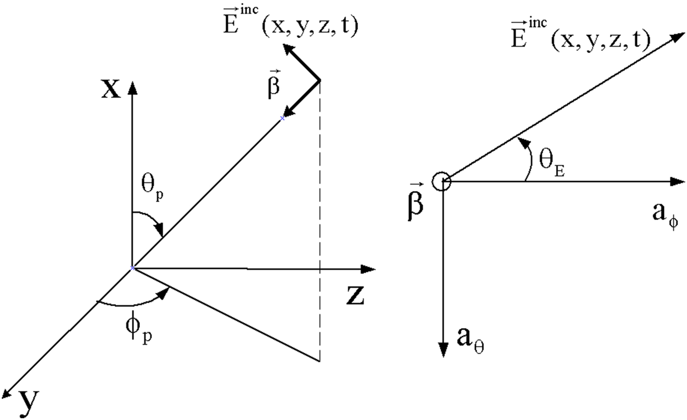
Fig. 3. Parameters setting of the incident field for the case of a uniform plane wave.
The incident field, in the absence of the line, can be written in the following frequency form (
 $\hat E_0 $
complex amplitude):
$\hat E_0 $
complex amplitude):
 $${\overrightarrow E}_i^{inc} \lpar x\comma \; y\comma \; z\comma \; \omega \rpar =\hat E_0 [{e_x \vec a_x+e_y \vec a_y+e_z \vec a_z }] e^{ - j\beta _x x} e^{ - j\beta _y y} e^{ - j\beta _z z} .$$
Wherein the projection coefficients of the unit vector of the incident field on the axes x, y, and z:
 $$\left\{\matrix{e_x=\sin \theta_E \sin \theta_P \cr e_y=- \sin \theta_E \cos \theta_P \cos \varphi_P - \cos \theta_E \sin \theta_P \cr e_z=- \sin \theta_E \cos \theta_P \sin \varphi_P - \cos \theta_E \cos \theta_P } \right..$$
The components of the wave vector are defined by its projection on different axes:
 $$\left\{\matrix{\beta_x=\beta \cos \theta_P \cr \beta_y=- \beta \sin \theta_P \cos \varphi_P \cr \beta_z=- \beta \sin \theta_P \sin \varphi_P } \right..$$
β is the phase constant related to the frequency and other properties of the medium by the following relation:
 $$\beta=\omega \sqrt {\mu \varepsilon }=\displaystyle{1 \over {\nu _0 }}\sqrt {\mu _r \varepsilon _r }\comma \; $$
with
 $\nu _0=\lpar 1/\sqrt {\mu _0 \varepsilon _0 } \rpar $
phase speed in the space.
$\nu _0=\lpar 1/\sqrt {\mu _0 \varepsilon _0 } \rpar $
phase speed in the space.
The medium is characterized by the permeability μ = μ 0 μ r and permittivity ε = ε 0 ε r .
B) MTL lossless modeling submitted to a plane wave
In what follows, we present a model that takes into consideration the field/line coupling. Depending on the Branin's model [Reference Branin14]: it permits to model the MTL lossless line, illuminated by a plane wave, through generators of voltage and current placed at the ends of the line in the time domain.
In the MTL lossless case, the system (3) becomes:
 $$\left\{\matrix{\displaystyle{{\delta V\lpar z\comma \; t\rpar } \over {\delta z}}+L\displaystyle{{\delta I\lpar z\comma \; t\rpar } \over {\delta t}}=V_F \lpar z\comma \; t\rpar \cr \displaystyle{{\delta I\lpar z\comma \; t\rpar } \over {\delta z}}+C\displaystyle{{\delta V\lpar z\comma \; t\rpar } \over {\delta t}}=I_F \lpar z\comma \; t\rpar } \right..$$
The modeling of the MTL with Branin's model requires decoupling of the equation system (10). This coupling is made by the modal method [Reference Paul1, Reference Rouijaa17, Reference Kane18].
In the modal base the system of equations (10) becomes:
 $$\left\{\matrix{\displaystyle{{\delta V_m \lpar z\comma \; t\rpar } \over {\delta z}}+L_m \displaystyle{{\delta I_m \lpar z\comma \; t\rpar } \over {\delta t}}=V_{Fm} \lpar z\comma \; t\rpar \cr \displaystyle{{\delta I_m \lpar z\comma \; t\rpar } \over {\delta z}}+C_m \displaystyle{{\delta V_m \lpar z\comma \; t\rpar } \over {\delta t}}=I_{Fm} \lpar z\comma \; t\rpar } \right..$$
L m and C m are diagonal matrices of dimension N × N:
 $$\left\{\matrix{L_m=T_V^{ - 1} .L.T_I \cr C_m=T_I^{ - 1} .C.T_V } \right..$$
And V Fm , I Fm are the voltage and current “forced” source victors in the modal base:
 $$\left\{\matrix{V_{Fm} \lpar z\comma \; t\rpar =T_V^{ - 1} V_F \lpar z\comma \; t\rpar \cr I_{Fm} \lpar z\comma \; t\rpar =T_I^{ - 1} I_F \lpar z\comma \; t\rpar } \right..$$
Matrices T V and T I are selected, so that the matrices L m and C m are diagonals.
After calculating the matrices L m and C m we determine the characteristic impedance and the delay associated with each line.
As in the case of conducted mode [Reference Mejdoub, Saih, Rouijaa and Ghammaz4, Reference Taylor, Satterwhite and Harrison11, Reference Rouijaa17], the modal electrical variables V m and I m of the MTL are related to each other by:
 $$V_m \lpar 0\comma \; t\rpar - Z_{Cm} I_m \lpar 0\comma \; t\rpar =V_{rm} \lpar l\comma \; t\rpar +E_{0m} \lpar l\comma \; t\rpar \comma \; $$
 $$V_m \lpar l\comma \; t\rpar - Z_{Cm} I_m \lpar l\comma \; t\rpar =V_{rm} \lpar 0\comma \; t\rpar +E_{lm} \lpar l\comma \; t\rpar .$$
With E 0 m and E lm are the voltage generators that model the plane wave coupling with the transmission line to the input and to the output line (Fig. 4): where
 $$V_{rm} \lpar l\comma \; t\rpar =V_m \lpar l\comma \; t - T_m \rpar - Z_{Cm} I_m \lpar l\comma \; t - T_m \rpar \comma \;$$
 $$V_{im} \lpar l\comma \; t\rpar =V_m \lpar 0\comma \; t - T_m \rpar - Z_{Cm} I_m \lpar 0\comma \; t - T_m \rpar \comma \;$$
and
 $$E_{0_m } \lpar l\comma \; t\rpar =V_{FT_m } \lpar l\comma \; t - T_m \rpar - Z_{Cm} I_{FT_m } \lpar l\comma \; t - T_m \rpar \comma \;$$
 $$E_{L_m } \lpar l\comma \; t\rpar =V_{FT_m } \lpar l\comma \; t\rpar - Z_{Cm} I_{FT_m } \lpar l\comma \; t\rpar . $$

Fig. 4. Line model submitted to a plane wave in the modal basis.
If we know the expression of the modal characteristic impedance Z Cm of the line and the delay T m associated with this line, then it will be easy to determine the “forced” generators E 0 m and E lm that model the influence of the incident field in the time domain. Their expressions are defined by [Reference Paul1]:
 $$E_{0_m } \lpar l\comma \; t\rpar =a_0 \left[{\displaystyle{{\varepsilon_0 \lpar t\rpar - \varepsilon_0 \lpar t - T_{rm} - T_Z \rpar } \over {T_{rm}+T_Z }}} \right]\comma \; $$
 $$E_{L_m } \lpar l\comma \; t\rpar =a_L \left[{\displaystyle{{\varepsilon_0 \lpar t - T_{rm} \rpar - \varepsilon_0 \lpar t - T_Z \rpar } \over {T_{rm} - T_Z }}} \right]\comma \;$$
where ε 0(t) is the amplitude of the electric field in the time domain, a 0 and a L are the coefficients depending on the parameters of the line defined by:
 $$a_0=\sum\limits_{k\;=\;1}^n {\lcub {[ {e_z T_{xyk} l - \lpar e_x x_k+e_y y_k \rpar \lpar T_{rml}+T_Z \rpar } ] [ {T_I^t } ]_{ik} } \rcub }\comma \; $$
 $$a_L=\sum\limits_{k\;=\;1}^n {\lcub {[ {e_z T_{xyk} l+\lpar e_x x_k+e_y y_k \rpar \lpar T_{rml} - T_Z \rpar } ] [ {T_I^t } ]_{ik} } \rcub }\comma \; $$
with
 $$T_{xyk}=\displaystyle{{x_k } \over {\nu _x }}+\displaystyle{{y_k } \over {\nu _y }}.$$
T z = l/ν z = lk z /ω, if a component wave that propagates along the axis T z = T rm , in the opposite case T z = 0.
If we insert equations (17.a) and (17.b) into equations (14.a) and (14.b), then we obtain:
 $$\eqalign{V_m \lpar 0\comma \; t\rpar - Z_{Cm} I_m \lpar 0\comma \; t\rpar & = V_{rm} \lpar l\comma \; t\rpar \cr & +\underbrace {a_0 \left[{\displaystyle{{\varepsilon_0 \lpar t\rpar - \varepsilon_0 \lpar t - T_{rm} - T_Z \rpar } \over {T_{rm}+T_Z }}} \right]}_{E_{0m} \lpar l\comma t\rpar }\comma \;} $$
 $$\eqalign{V_m \lpar l\comma \; t\rpar - Z_{Cm} I_m \lpar l\comma \; t\rpar &=V_{rm} \lpar 0\comma \; t\rpar \cr & +\underbrace {a_L \left[{\displaystyle{{\varepsilon_0 \lpar t - T_{rm} \rpar - \varepsilon_0 \lpar t - T_Z \rpar } \over {T_{rm} - T_Z }}} \right]}_{E_{lm} \lpar l\comma t\rpar }}.$$
From equations (19.a) and (19.b) we can deduce the equivalent circuit of Fig. 4.
The relationship between the voltage and current modal vectors and real ones is given by the following expressions in the form of the voltage and current generators placed at the ends of each conductor:
 $$\eqalign{& V\lpar z\comma \; t\rpar =\sum\limits_{k\;=\;1}^n {T_{Vik} V_m \lpar z\comma \; t\rpar \comma \; } \cr & \quad I_m \lpar z\comma \; t\rpar =\sum\limits_{k\;=\;1}^n {T_{_I }^{ - 1} I\lpar z\comma \; t\rpar } .}$$
Equations (19a), (19b), and (20) provide a representation of an equivalent circuit model. The advantage of this model is that it is valid in both the time and frequency domains for linear and nonlinear loads.
III. SIMULATION AND RESULTS
In this part of simulation, we will first discuss the case of a referenced MTL line in relation to a reference conductor submitted to a plane wave to validate the coupling model line/wave. Later, we will see the incident variation effects on an MTL line.
A) Coupling mode validation
We consider a cable of three conductors from length 2m immersed in a dielectric. The conductor “0” is used as a reference (Fig. 5). They are loaded by a 500 Ω impedance network. These three conductors are submitted vertically to polarized plane wave (Ex), with kz propagation horizontal direction. The variation of the electric field is defined by a ramp rise time tr = 1 ns (Fig. 5).

Fig. 5. Geometric configuration of a mono-wire line submitted to a horizontally polarized plane wave.
In this example, we have studied the influence of the perturbation wave on the two conductors in the time and frequency domains.
The linear line parameters L and C were calculated from the geometry of the mono-wire line (Fig. 5).
 $$\eqalign{& L=\left[{\matrix{ {7485} & {2408} \cr {2408} & {7485} \cr } } \right]\lpar {\hbox{nH/m}} \rpar \; \cr & \quad C=\left[{\matrix{ {24{\kern 1pt} {\kern 1pt} 982} & { - 6266} \cr { - 6266} & {24\, 982} \cr } } \right]\lpar {\hbox{pF/m}} \rpar .}$$
1) TRANSIT ANALYSIS
In Fig. 6, we visualize the observed voltage through the conductor ends n°1 and the results are obtained by the analytical method [Reference Paul8]. Figure. 6 shows a good agreement, the far-crosstalk voltage resembles a form of stairs due to the phenomenon of reflection. The width of each level is equal to twice the propagation time of the line (come-back signal).

Fig. 6. Induced voltage on conductor n°1:Esacap2000 simulation results and analytical method results taken from [8].
2) FREQUENCY ANALYSIS
In Figs 7 and 8, we visualize the amplitude and phase of the far-crosstalk voltage on the conductor no. 1 and the results are obtained by [Reference Paul8] using the analytical method. This time, the three conductors are submitted to a sinusoidal incident field of amplitude 1 V/m. Figures 7 and 8 are in good agreement. The near-crosstalk voltage presents anti-resonances that occur when the length line is a multiple of the wavelength.

Fig. 7. Induced voltage amplitude on the conductor n°1 simulated by Esacap2000 and analytical method results taken from [8].

Fig. 8. Induced voltage phase on the conductor n°1 simulated by Esacap2000 and analytical method results taken from [8].
B) Incident angle variation
To study the influence of the incident variation of the perturbation wave on the transmission line, we take a referenced line in relation to a ground plane (Fig. 9), a conductor of radius r w = 10 mils and of length L = 1 m suspended at a height h = 2 cm above a ground plane.
Fig. 9. Geometric configuration of a referenced line in relation to a ground plane is submitted to a horizontally polarized plane wave.
Terminators are resistive with R S = 500 Ω and R L = 1000 Ω. This conductor is submitted to a uniform plane wave (E x ).
The variation of the electric field is defined by a ramp rise time tr and the amplitude E 0 = 1 V/m (Fig. 10).
Fig. 10. Electric field variation is defined by ramp rise time tr = 1 ns.
The characteristic impedance of the line Zc = 303.34782 Ω and the delay Tr = 3.33564 ns.
In Fig. 11, we represent the amplitude variation voltage at the input of the line as a function of frequency by setting the angle that gives the direction of propagation in relation to the axis Oz (φ p = cte), and vary the incident angle between ±90°. Figure 12 shows the zoom in the maximum amplitude voltage from Fig. 11 to visualize the difference between the curves.
 $$\eqalign{&\theta _L=\displaystyle{{ - \pi } \over 2}\comma \; \matrix{ \cr } \theta _J=\displaystyle{{ - \pi } \over 3}\comma \; \matrix{ \cr } \theta _I=\displaystyle{{ - \pi } \over 4}\comma \; \matrix{ \cr } \theta _H=\displaystyle{{ - \pi } \over 6}\comma \; \matrix{ \cr } \theta _G=0\comma \; \matrix{ \cr } \cr & \theta _F=\displaystyle{\pi \over 6}\comma \; \matrix{ \cr } \theta _E=\displaystyle{\pi \over 4}\comma \; \matrix{ \cr } \theta _D=\displaystyle{\pi \over 3}\comma \; \matrix{ \cr } \theta _B=\displaystyle{\pi \over 2}}$$

Fig. 11. Amplitude variation as a function of the angle θ (φ = cte).

Fig. 12. Maximum amplitude variation as a function of the angle θ.
Figure 12 shows the maximum amplitude voltage variation at the line input in function of the angle θ p. We note that the voltage is more important for the case where the angle equals zero, this value decreases in the case where the angle tends to ±90°. We note that there is a symmetry in the values of the angle to 0° (Fig. 12). The amplitude distribution indicates that the voltage is greater toward the central value of 0° and less important toward the ends.
IV. CONCLUSION
In this paper, a variation effect of the incident angle on an MTL line is presented through the use of a model coupling of a transmission line with a plane wave valid in both the time and the frequency domains. This model is based on the characteristics method (Branin method), and is implemented by the ESACAP circuit simulator. The model of a transmission line referenced to a ground plane, which is excited by an external plane wave, has been studied, and the amplitude distribution has shown that the voltage is more important toward the center value of 0° and less important toward the ends.
 Youssef Mejdoub was born in Morocco, in 1980. He obtained his Ph.D. thesis on “Inter-equipment Electromagnetic compatibility, applications: Multiconductor Transmission Lines Modeling”, in June 2014, from Cadi Ayyad University – Marrakesh Morocco. He received the DESA (6 years study after the baccalaureate) in Telecommunications & Network from Cadi Ayyad University, in 2007. His research interest includes the electromagnetic compatibility, multiconductor transmission lines, and telecommunications.
 Hicham Rouijaa is a Professor of physics, attached to Hassan 1 University, Morocco. He obtained his Ph.D. thesis on “Modeling of Multiconductor Transmission Lines using Pade approximant method: Circuit model”, in 2004, from Aix-Marseille University – France. He is an associate member of Electrical Systems and Telecommunications Laboratory LSET at the Cadi Ayyad University. His current research interests concern electromagnetic compatibility and multiconductor transmission lines.
 Abdelilah Ghammaz received his Doctor of Electronic degree from the National polytechnic Institute (ENSEEIHT) of Toulouse, France, in 1993. In 1994 he went back to Cadi Ayyad University of Marrakech – Morocco. Since 2003, he has been a Professor at the Faculty of Sciences and technology, Marrakech, Morocco. He is a member of Electrical Systems and Telecommunications Laboratory LSET at the Cadi Ayyad University. His research interests in the field of electromagnetic compatibility, multiconductor transmission lines, telecommunications, and antennas.