I. INTRODUCTION
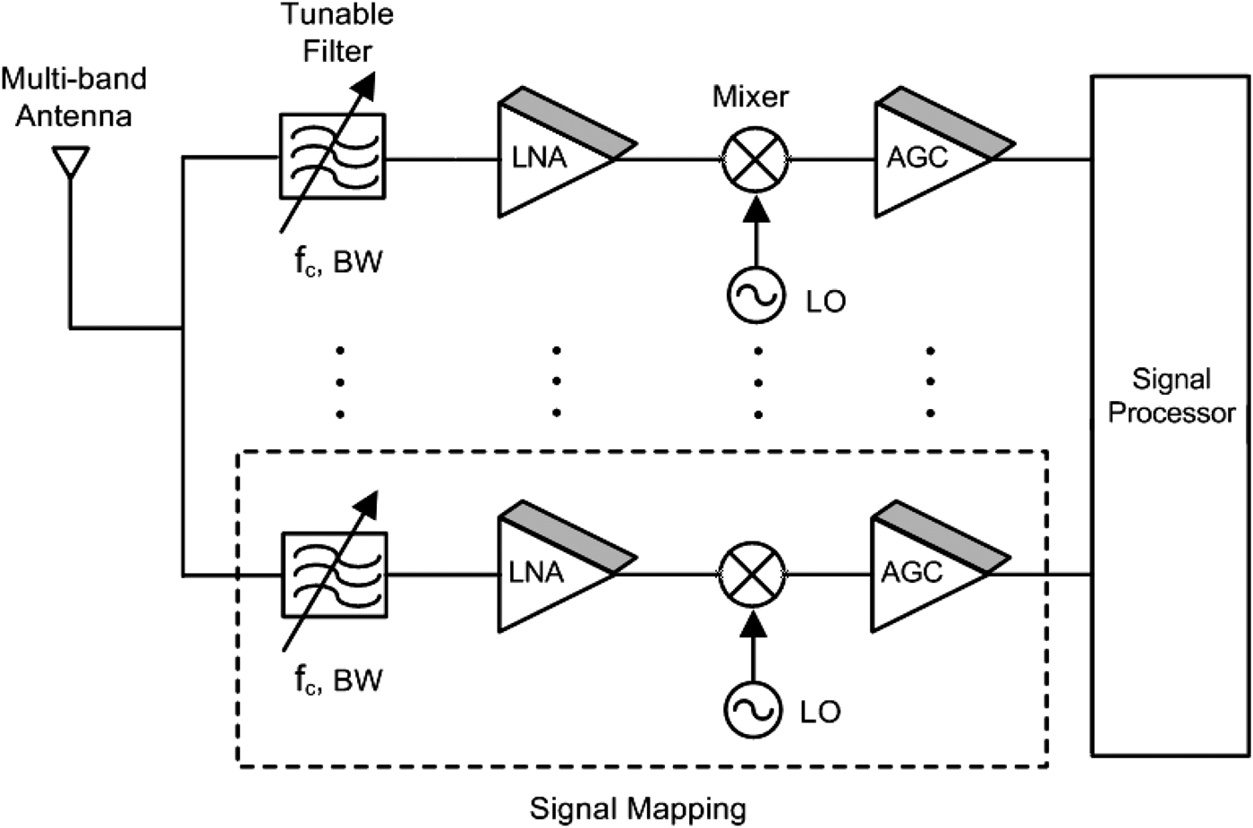
With the tremendous growth of wireless communication systems, cognitive radio technologies have increasingly been developed because of their ability to adaptively utilize the available spectrum [Reference Mitola1–Reference Choi5]. Since licenced spectrum resources are often not fully exploited, many spectrum-sensing methods have been studied [Reference Li, Wang, Horng and Peng6–Reference Berezdivin, Breinig and Topp8]. Often times it is assumed that the transmitter and receiver frequencies will move to an open spectrum; however, an alternative is to stay in the designated band and adapt the radio frequency (RF) hardware. Once a system senses an unoccupied spectrum, it would be essential to know how the system throughput can be maximized for a given radio environment. The purpose of signal mapping is to scan the spectrum as a function of system parameters and optimize the parameters to improve the wireless performance. One optimizable parameter is the state of the preselect filtering. The system throughput is estimated through signal mapping and then system parameters, such as the frequency and bandwidth of the tunable preselect filter, are updated. Therefore, the tunable preselect filter is reshaped based on the feedback from signal mapping. Figure 1 shows an example of such a receiver with multiple receiver chains.

Fig. 1. Tunable front-ends having a signal mapping. One maps the signal throughput and the others react.
Tunable preselect filters are important components in wireless communication system [Reference Nath9–16]. One of the known examples of using a tunable filter is a broadcast television where the tunable filter is simply tuned to be centered around a wanted channel without any intelligent tuning functionality. However, the tunable filter can be smarter if it is dynamically tuned based on a given spectrum. The big advantage of having the tunable preselect filter is that it can adjust the filtering shape to adapt to a spectral environment. In particular, the flexibility of preselect filtering allows us to reduce the surrounding interference. For example, a moving vehicle will encounter many different spectral interferers as it moves through a city. When it goes specially closer to transmitters such as high-power cellular phone towers or television transmitters, the tunable preselect filter can be aware of the spectrum and optimize the filtering to maximize the receiver performance. We have designed and fabricated tunable preselect filters with a wide range of tuning and low insertion losses using evanescent-mode cavity resonators [Reference Joshi, Sigmarsson, Moon, Peroulis and Chappell17]. In this paper, the effect of these tunable preselect filters on a fielded wireless communication system is numerically and experimentally evaluated. In addition, application guidelines toward filtering strategies are described to help the wireless system designers to understand the advantages and best usage of tunable preselect filters.
A) Testbed and motivation
In order to demonstrate the impact of a tunable preselect filter on wireless communication systems, we installed the tunable filter in a fielded wireless sensor network [Reference Montestruque and Lemmon18] which has been deployed in the mid-sized city of South Bend, Indiana, USA. In this network, 150 wireless sensor nodes were widely distributed throughout the city to dynamically monitor and sequentially divert sewer flow to the river or sewer treatment plant depending on its contamination level [Reference Montestruque and Lemmon18]. After installation of all of the nodes, interestingly, five nodes were electrically “lost” with little to no packet reception. This failure was not because of low signal strength at these nodes but because strong interference significantly degraded the mote reception. For instance, the difference between problematic and normal areas in terms of the packet reception rate (PRR) was 97% in spite of the similar received signal strength indicator (RSSI) level of −45 dBm. We define the PRR as successful packet reception based on the comparison with known data transmission. The proximity of GSM cellular phone towers near the problematic area was found to be the correlating factor for the lost nodes.
Conventional knowledge and practice indicates that a preselect filter should be centered around the middle of a device's receive band [Reference Yeung and Wu19–Reference Hong and Lancaster21]. However, when the surrounding interference is close to one edge of the receive band, we have found that dynamic “offset” placement of the preselect filter provides interference mitigation and significantly improves PRR. In other words, the passband of the preselect filter is moved slightly away after identification of the interferers existence. Since interference is in general unpredictable and time-varying, it is better to have an intelligent system with a tunable filter that can adapt to its interfering environment. Within a wireless sensor network it is often unpredictable where the mote will be placed, let alone what the interferers will be for a given placement. It is preferable to have an adaptable system that adjusts after placement of the node or continuously. Previously, we demonstrated a tunable center frequency high-Q filter and showed basic improvements in the PRR [Reference Jeong and Chappell22]. In this paper, we show the effect of tunable bandwidth as well as a more thorough analysis of the effect of both tunable features. We analyze adaptive filtering at a deeper level with simulation as well as measurement. In total, we show that a combination of the center frequency tuning with bandwidth tuning allows for substantially better results. We also explore the tradeoff in finding the optimal setting of the tunable preselect filter. Useful guidelines for tuning the preselect filter in a specific electrical environment are described.
II. ANALYSIS
In our project, the wireless sensor network is connected to the GSM network to send the environmental data to a control center. There is a final gateway that can communicate to the GSM tower; however by getting closer to the tower, the motes are more susceptible to out-of-band interference from the GSM system. Through the outdoor measurement, we found that the interfering GSM signal significantly degrades our system because it is closely located to the Industrial, Scientific and Medical (ISM) band, which is used for communication between the non-gateway nodes. The widely distributed interferers with high-power levels created signal distortion and corrupted the desired signal by generating the third-order intermodulation product that appeared in the mote's receive band, saturating the receiver. The typical interference patterns were monitored and repeated in controlled environments to have control of the interference for analysis.
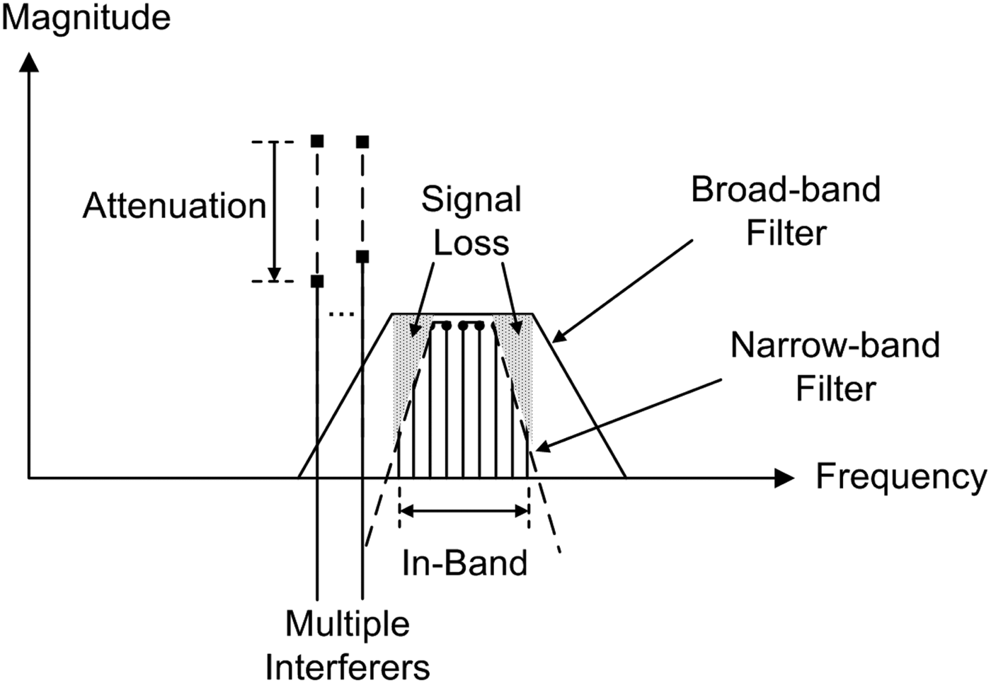
In response to these interference sources, the bandwidth and center frequency of the tunable preselect filter were adjusted to attenuate the interference and achieve the best PRR. Figure 2 illustrates the tradeoff between interference attenuation and signal loss when the filter's bandwidth was reduced to less than the band of the receive signal in an attempt to reject the high-power interference signal. Since the receive signal is frequency hopping through the band with a uniform distribution, changing the filter's bandwidth and center frequency reduces the received signal level and limits the signal-to-noise ratio (SNR). However, in all cases in the wireless sensor network we used, and it was found that the receive signal's SNR was large enough not to be the limiting factor. Therefore, the benefits of mitigating strong interferers by partially filtering the receive band strongly outweigh the accompanying reduction in SNR.
Fig. 2. Tradeoff between signal loss and interference attenuation when the bandwidth of the tunable filter becomes narrow.
In our study, we present four cases that illustrate how the tunable filter improves system performance. Those cases are described as follows:
1) Reference: The wireless sensor network was set up in an anechoic chamber to obtain reference data without interferers.
2) Controlled interference: Also in the anechoic chamber, isolated interferers were introduced to mimic the interference from the largest signals which are observed in our testbed.
3) Background outdoor interference: The wireless sensor network was set up outdoors. The background interference was measured and recorded.
4) Controlled interference with background outdoor interference: Along with the background interference, single or multiple interferers were introduced to simulate the measured radio environment based on the previous measurements seen in the field. This case represents interference sources that are in close proximity to the sensor network.
This systematic study has characterized the effect of preselect filter bandwidth and filter center frequency on the PRR of the system in the presence of a strong interference source.
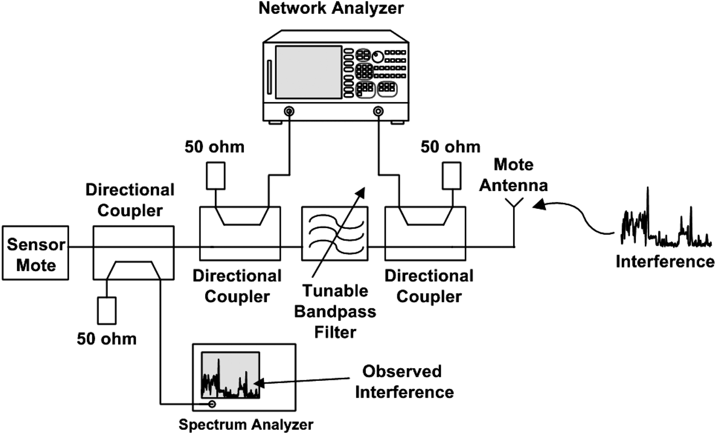
As mentioned previously, the tunable preselect filter is a high-Q, tunable, evanescent-mode cavity filter. The combination of narrow bandwidth and frequency tunability was made possible through the use of piezoelectric actuators that externally adjust the cavities' dimension in a substrate as described in [Reference Joshi, Sigmarsson, Moon, Peroulis and Chappell17]. The distinguishing factor is the relatively high-Q of the filter despite its wide tuning range. An unloaded Q of 298 is measured at 916 MHz despite the capability of tuning over an octave in frequency and dynamically changing the bandwidth. This high-Q allows for 1.9 dB of the insertion loss at the widest bandwidth. Also, the Q is important so that the sensitivity is not sacrificed despite the ability to remove interferers. The fractional bandwidth tuning is 42%. Despite the wide tuning range, we are only using a fraction of the tuning range for this fixed frequency network for this study. The variable bandwidth and center frequency were adjusted to study PRR. In order to monitor the filter response in real time, a network analyzer (Agilent 8720ES) and two broadband 10 dB directional couplers were utilized at both sides of the tunable filter. The setup allows for concurrent monitoring of the interference and the shape of the filter. Incoming interference and desired signal were monitored through another directional coupler connected to a spectrum analyzer (Agilent E4408B), as shown in Fig. 3. By using this setup, the interference attenuation, RSSI, and PRR were measured, so that the resulting packet rate can be compared to the interference spectrum and filter state at the time of the measurement.
Fig. 3. Sensor network measurement setup with real-time filter tuning.
A) Filter bandwidth
One mechanism for having an intelligent front end would be to have selective bandwidth control on the preselect filter. To study the benefit of this dynamic tuning, we varied the bandwidth for a variety of receive spectra. In general, a wider bandwidth would be preferred because the noise figure of the receiver would be the lowest. However, in the presence of an interferer, it would be possible to decrease the bandwidth to protect the receiver, at the sacrifice of increased loss and noise.
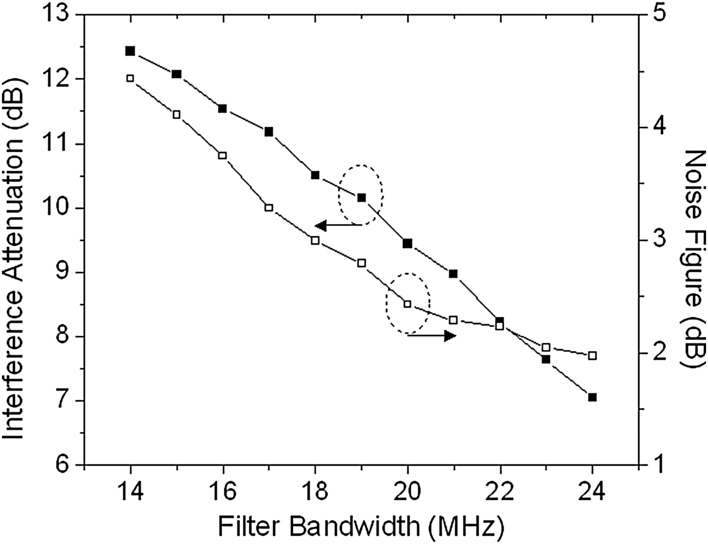
The bandwidth of the filter can vary from 14 to 24 MHz. The interference attenuation and noise figure of the tunable filter are shown in Fig. 4 as a function of the filter bandwidth. The attenuation difference at 894 MHz between the widest and narrower bandwidth was 7.2 dB as shown in Fig. 4. The tradeoff is that the noise figure increases as the filter bandwidth decreases. Therefore, the SNR is important for the lower bandwidth, whereas signal-to-interference ratio (SIR) is critical for the wider bandwidth.
Fig. 4. Tradeoff between interference attenuation at 894 MHz and noise figure for tunable bandwidth filter design with Q = 298.
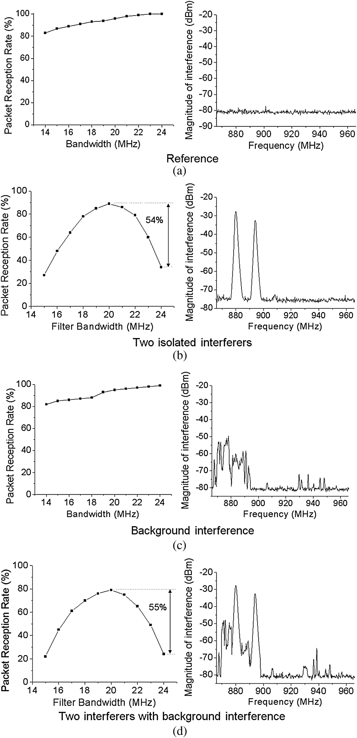
The PRR of the system was measured while adjusting the filter bandwidth as shown in Fig. 5(a). The measured result shows that in the absence of strong interference, the PRR decreases as the filter bandwidth decreases, as expected. This is due to the increased noise in the system as the bandwidth is dynamically decreased. To mimic the interferers observed in our testbed, two Gaussian Minimum Shift Keying (GMSK)-modulated signals in Fig. 5(b) were induced at 894 and 880 MHz with −32 and −27 dBm, respectively, based on what we measured at the testbed. Although the expected increase in bandwidth provided a nearly linearly better packet rate as shown in Fig. 5(a), the presence of interferers clearly shows an optimal operating point in the presence of interferers. The optimal bandwidth to achieve the best PRR was found to be 20 MHz while keeping the filter center frequency at the center of the band of interest. This indicates that even significant signal attenuation within the receive band is preferable to having the filter with the widest bandwidth in the presence of large interfering signals although the filtering effectively cuts off the hopping range of the band by placing the cutoff frequency squarely in the center of the band of interest. A 54% improvement in PRR was achieved compared to the widest filter state.
Fig. 5. Effect of the filter bandwidth. Maxhold was used to capture the interference spectrum.
With this study in mind, the outdoor measurement was carried out with existing background interference, as shown in Fig. 5(c). This case represents when the network is not close to a GSM broadcasting station but multiple GSM stations exist. The measurement result shows that, in this scenario, keeping the bandwidth wide is the best way to maintain the highest reception rate, because the magnitude of the low-level background interference is negligible based on our previous work [Reference Jeong and Chappell22]. Therefore, SNR was the limiting factor. Figure 5(d) shows the PRR when the two interferers of Fig. 5(b) were added on top of the background interference of the outdoor measurement. These signals significantly degraded the radio performance because they increase signal distortion as well as the intermodulation distortion (IMD) which falls on top of the band of interest. Therefore, the PRR is not simply a function of signal distortion but a combination of signal distortion and the IMD. The measurement result shows that the PRR was improved by 55% at 20 MHz compared to the widest bandwidth.
B) Filter center frequency
The most intuitive approach to setting the center frequency of a receive filter would be to position the filter in such a way that the filter is centered around the receive band, thereby keeping the desired receive signal power as high as possible. However, the experimental results found that this is often suboptimal in the presence of strong interferers. We found in such cases that an off-center filter placement elicited better system performance, even at the expense of cutting off a portion of the hopping frequency range.
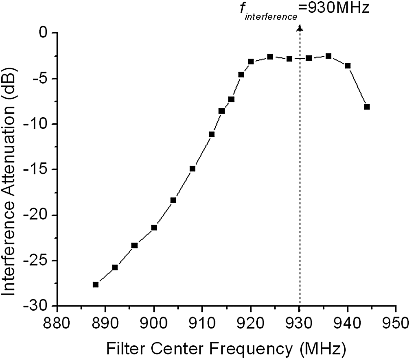
For example, in one problematic area within our fielded sensor network, we found that a single strong interferer that is very close to the band of interest could significantly lower the PRR. This interferer was presumably from narrowband personal communication service (PCS) or commercial mobile radio service (CMRS) [23, 24]. For this case, we hypothesized that it would be advantageous for the system to adjust the filter center frequency to significantly attenuate the interferer. The interference attenuation at 930 MHz was measured and shown in Fig. 6. In addition, we studied the effect of adjusting filter center frequency in the same measurement situation as was performed in the case of filter bandwidth.
Fig. 6. Interference attenuation as a function of the filter center frequency when interference is located at 930 MHz.
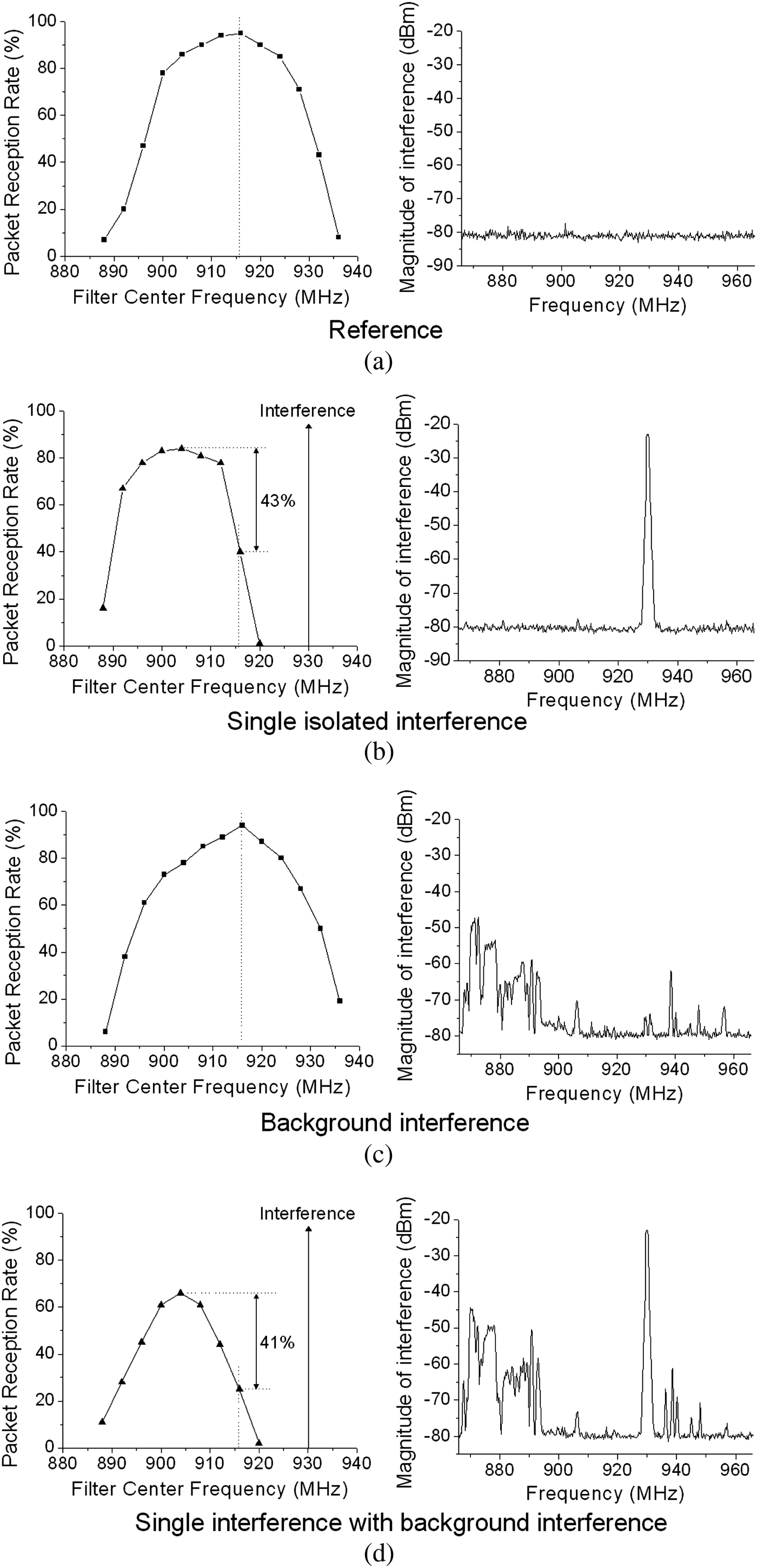
First, in the anechoic chamber with no interfering radiation, we found that the optimal position of the filter center frequency was at the center of the band of interest, because the filter should attenuate the signal as little as possible to achieve the best PRR as shown in Fig. 7(a). Next, when a single isolated interferer of −23 dBm was induced at 930 MHz, the optimal filter center frequency was shifted to 904 MHz which is 12 MHz off from the center of the band. The PRR was increased by 43% compared to the center-positioned filter as illustrated in Fig. 7(b).
Fig. 7. Effect of the filter center frequency.
In the fielded system, when negligible background interference exits, the best location for the highest reception rate was the center of the band of interest as we predicted, as shown in Fig. 7(c). However, when strong interference was introduced, the optimal filter center frequency to achieve the best PRR was shifted off center to 904 MHz. The difference between the optimal and centered frequency was 41% in PRR. Therefore, there is clear benefit for the system to move the filter center frequency in the presence of close and strong interference.
C) Effect of location of interference
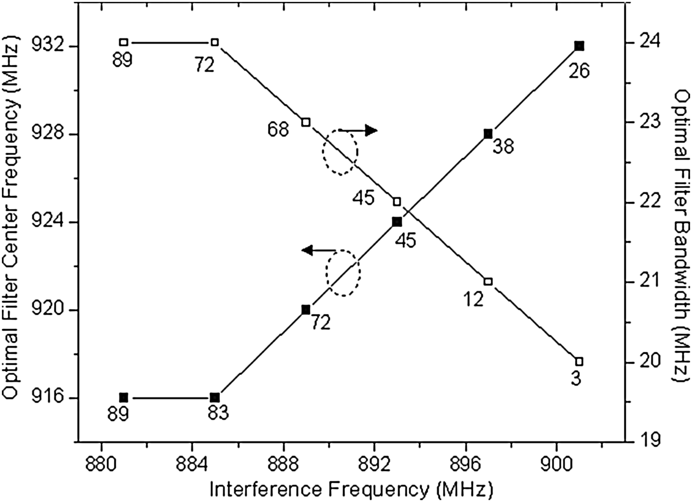
In general, since the frequency of GSM interference can be arbitrary over the service band, the effect of interference location was investigated as a function of interference frequency. An interferer of −30 dBm was introduced and moved from 881 to 901 MHz. The optimal filter center frequency and bandwidth were determined by finding the highest PRR as shown in Fig. 8. The conventional filter was the optimal filter when the interference is located below 885 MHz because the receiver is not limited by either interference or noise. However, the optimal center frequency and bandwidth varied when the interference comes closer to the band of interest. When the interference is at 901 MHz, which is 1 MHz beside the ISM band, the optimal filter center frequency and bandwidth were 932 and 20 MHz, respectively, achieving 26 and 3% in PRR. The measured result indicates that the optimal filter bandwidth decreases as interference comes closer to the band of interest. Similarly, the optimal filter center frequency was shifted away from the interferer depending on the location of the induced interference. Thus, it was demonstrated that adaptively adjusting the filter bandwidth or center frequency based on the proximity to interference gives the clear advantage of improving the PRR despite sacrificing the desired signal.
Fig. 8. Optimal filter center frequency and bandwidth as a function of frequency of interference. The PRR for each measured optimal location is labeled for each data point.
The effect of tuning each independent variable has been shown in Figs 5, 7, and 8. However, full optimization of the tunable bandwidth and frequency is a multivariable problem which needs a two-dimensional (2D) mapping. By using the measurement system, the full 2D packet rate was measured versus filter center frequency and bandwidth. The frequency was shifted at increments of 4 MHz and then bandwidth was changed from 14 to 24 MHz with increments of 1 MHz. Mapping the full measurement allows us to understand and analyze the globally optimal position for the filter and compare the mechanisms to search for this optimum in a given spectrum. The 2D mapping is the subject of the next section.
D) Two-dimensional filter analysis
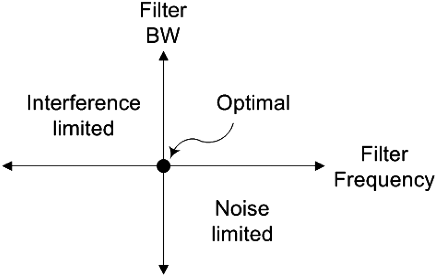
Our hypothesis was that there are optimal filter parameters that can be used to achieve a maximum PRR depending on the filtering shape. Intuitively, we predict that as the filter frequency moves away from the interference the mote receiver is limited by noise due to a reduction in signal power; meanwhile, if it moves toward the interference the receiver is limited by the interference owing to small attenuation. Similarly, as the filter bandwidth increases, the receiver will be interference-limited because of a lack of interference attenuation, and, as the bandwidth decreases the receiver is noise-limited due to relatively high insertion loss. These trends are predicted as a function of the filter bandwidth and frequency as shown in Fig. 9. At the system level, this effect of filter frequency and bandwidth can be explained with signal-to-noise-plus interference ratio (SNIR). SNIR is defined as the ratio of signal power to the combined noise and interference power [Reference Turkboylari and Stuber25, Reference Hamdi26]. Each power is written as a function of filter frequency and bandwidth. Thus, the SNIR is written as below.
Fig. 9. Notional trends for the optimal filtering point and limiting factors as a function of the filter bandwidth and frequency for an interferer lower in frequency than the band of interest.
 $$SNIR=\displaystyle{{P_{SIGNAL} \lpar f_c\comma \; BW\rpar } \over {P_{NOISE} \lpar f_c\comma \; BW\rpar +P_{INTERFERENCE} \lpar f_c\comma \; BW\rpar }}$$
where P is the averaged power. This formula indicates that the SNIR is proportional to signal power, whereas it is inversely proportional to noise and interference power. The degree of the incremental power change varies depending on the frequency shift and bandwidth variation. For example, if the filter bandwidth is narrower, the signal strength is reduced by insertion loss. Also, the noise power increases and the interference power decreases. Thus, an optimal filtering point can be achieved by tradeoff of these powers. We show an example of optimal filtering in the next paragraphs.
In order to explore these trends further, the wireless sensor network was modeled based on our measurement. A system-level simulation using Agilent advanced design system (ADS) was performed. An FM-modulated mote signal was generated and programmed to be hopped over the mote's receive band. For an interferer, a single GSM saturation tone was also generated at 894 MHz and summed with the mote signal through a combiner. The insertion loss and shape of the tunable preselect filter was modeled according to the measurement. Since the frequency spectrum in simulation fully includes the change in frequency response of the filter, interference, and mote signals, the observation bandwidth was chosen to be 150 MHz. In other words, the simulation time step is set to be 6.67 ps. To sufficiently sample the time-domain signal through the band-pass and low-pass filter, the impulse response time of the filters was defined by 20/(BW) [Reference Zverev27, Reference Blinchikoff and Zverev28]. The gain compression due to the strong interferer was modeled with the 1-dB compression point of −11 dBm in an low noise amplifier (LNA). The overall system performance was estimated by observing the PRR. The designed schematic is shown in Fig. 10. Since this modeling is approximately modeled based on the measurement on board, it does not consider electromagnetic couplings between the chipsets and transmission lines. In the system-level simulation, we scanned the frequency and bandwidth of the tunable preselect filter over the band of interest by measuring PRR as same as the experiment. Similarly, we experimentally measured the PRR as a function of both filter parameters and compared with the simulation result, as shown in Fig. 11.
Fig. 10. System-level simulation with ADS. Mote signals are frequency hopping over the ISM band and a GSM signal is an interferer against the mote signal. Packet error rate (PER) is measured by comparing the original mote signal with the demodulated signal. PRR is obtained by (1-PER).
Fig. 11. Comparison of simulated and measured results.
This mapping process allowed us to find where the tunable preselect filter should be positioned to achieve maximum PRR and to estimate how much the system throughput can be improved for a current spectral environment. The simulated result indicates that the maximum PRR was achieved when the filter bandwidth is 19 MHz and the filter center frequency is 924 MHz. Comparison to the measured results, indicates that the measured optimal filter center frequency was 0.2 MHz away from the simulated optimal frequency and the measured optimal filter bandwidth was 22 MHz, which is 3 MHz off from the simulated optimal point. These results in general predict what was measured with slight variations based on the difficulty of the system simulation technique to model the RF components exactly, such as mismatches that might occur between components.
Based on the measured results, we can explore different possibilities for finding the optimal point. This study allowed us to understand how the tunable preselect filter might be varied in the field in order to determine the maximum packet rate versus the variable of bandwidth and frequency. When we subsequently optimize each variable, it is instructive to see how far off of the optimal packet rate these quick approaches are. We tested two simplified filtering schemes. When the filter center frequency is first adjusted and the filter bandwidth is changed next, we define this scheme as f c → BW. The filter moves to A and then B as shown in Fig. 12. Similarly, the bandwidth is adjusted first followed by the center frequency; we define this as BW → f c which moves to C then D. The change started from the conventional filtering point where the filter is centered at the center of the receiver band with 24 MHz of the maximum bandwidth, which is the best case for a static filter. In practice, however, static filters are rarely, if ever this tight around the frequency band due to tolerance issues. The optimal position of the filter achieved PRR by 59% over the conventional static filter, which is frequency-centered with the widest bandwidth.
Fig. 12. Measured results of PRR for different paths.
Table 1 illustrates measured PRR at each filtering point in Fig. 12. Each point substantially increases the PRR performance over the conventional static filter, which is the strongest message from Table 1. The overall maximum PRR at the optimal position was measured to be 68% while the conventional static filter achieved only 9%. Among the 2D filtering schemes, f c → BW achieved only 3% higher PRR than BW → f c. However, the PRR at A (frequency tuning only) was 10% higher than that at C (bandwidth tuning only). This shows that if only one variable were tuned, for this data it is clear that the tuning of the center frequency is desirable. Thus, we concluded that the 2D adaptive algorithm is inevitable to reach the overall maximum PRR, however, sequential optimization gives the bulk of the benefit. The optimal algorithm is out of the scope of this paper, but this study demonstrates that there are substantial gains to be had by maturing the frequency and bandwidth trade space. The optimal point can be easily determined because of the maximum peak. Thus, it is obvious that the system performance depends on how to optimize the filtering schemes.
Table 1. Measured packet reception rate at each filtering point.

III. CONCLUSION
The effect of tuning the bandwidth and frequency of a tunable filter in a fielded wireless network was demonstrated in the presence of interferers. By adjusting the filter bandwidth and/or the center frequency, the PRR was significantly improved. The 900 MHz unlicenced band was studied as a useful representative narrowband system. In particular, the PRR was improved by more than 50% while tuning the filter bandwidth. Also, the PRR was increased by more than 40% by tuning the filter center frequency. By using the combined method, 68% of PRR was improved. The measurement was verified through a system-level simulation analysis and application guidelines for an optimal filtrating scheme were presented for a typical interferer configuration. Both the filter frequency and bandwidth were determining factors in achieving the maximum PRR. Therefore, design of the capability to tune both seems appropriate for cognitive systems, particularly, an interference-crowded radio environment.
ACKNOWLEDGEMENTS
This work was supported by the DARPA (Defense Advanced Research Projects Agency) Analog Spectral Processors grant. The authors would like to thank Hjalti Sigmarsson and Himanshu Joshi for help with the tunable filter.
 Seongheon Jeong received the B.S. degree in Radio Science and Engineering from the National Korea Maritime University at Busan, in 2000 and the M.S. degree in Electrical and Electronic Engineering from the Yonsei University at Seoul, in 2002. He received the Ph.D. degree at Purdue University in West Lafayette, IN in the USA, in 2010. He is currently working at Research In Motion, Inc. His current interests are reconfigurable radio components, microwave systems, and antennas.
 William J. Chappell received the B.S.E.E., M.S.E.E., and Ph.D. degrees from the University of Michigan at Ann Arbor in 1998, 2000, and 2002, respectively. He is currently a Professor with the School of Electrical and Computer Engineering, Purdue University, West Lafayette, IN. His research focus is on advanced applications of RF and microwave components. He has been involved with numerous federal and state funded projects involved in advanced packaging and material processing for microwave applications. His research sponsors include the Homeland Security Advanced Research Projects Agency (HSARPA), Office of Naval Research (ONR), the National Science Foundation (NSF), the State of Indiana, Communications – Electronics Research, Development and Engineering Center (CERDEC), and Army Research Office (ARO), as well as industry sponsors. His research group uses electromagnetic analysis, unique processing of materials, and advanced design to create novel microwave components. His specific research interests are the application of very high-quality and tunable components utilizing multilayer packages. In addition, he is involved with high-power RF systems, packages, and applications. Dr. Chappell was the IEEE Microwave Theory and Techniques Society (IEEE MTT-S) Administrative Committee (AdCom) secretary in 2009 and treasurer from 2011 to 2012. He was a member of the IEEE MTT-S AdCom from 2010 to 2012.