


1. Introduction
The characterization of the viscoelastic properties of colloidal suspensions has long been the subject of fundamental research due to the ubiquity of such suspensions in biology and industry. Microrheological techniques have been widely employed for such measurements due to their advantages in probing the local material response in systems such as porous media (Cai, Panyukov & Rubinstein Reference Cai, Panyukov and Rubinstein2011; Di Rienzo et al. Reference Di Rienzo, Piazza, Gratton, Beltram and Cardarelli2014; Wang et al. Reference Wang, Ackerman, Slowing and Evans2014; Begam et al. Reference Begam, Chandran, Sprung and Basu2015), biological systems (Ramadurai et al. Reference Ramadurai, Holt, Krasnikov, van den Bogaart, Killian and Poolman2009; Parigi et al. Reference Parigi, Rezaei-Ghaleh, Giachetti, Becker, Fernandez, Blackledge, Griesinger, Zweckstetter and Luchinat2014; He et al. Reference He, Song, Su, Geng, Ackerson, Peng and Tong2016) and microfluidic devices (McWhirter, Noguchi & Gompper Reference McWhirter, Noguchi and Gompper2009; Frydel & Diamant Reference Frydel and Diamant2010; Shani et al. Reference Shani, Beatus, Bar-Ziv and Tlusty2014; Misiunas et al. Reference Misiunas, Pagliara, Lauga, Lister and Keyser2015; Huang et al. Reference Huang, Gawlitza, von Klitzing, Steffen and Auernhammer2017). Research has shown that the viscoelastic properties of a colloidal suspension are strongly affected by the confining boundaries (Caruso et al. Reference Caruso, Grieser, Murphy, Thistlethwaite, Urquhart, Almgren and Wistus1991; Ouali & Pefferkorn Reference Ouali and Pefferkorn1996; Dufresne et al. Reference Dufresne, Squires, Brenner and Grier2000; Wille et al. Reference Wille, Valmont, Zahn and Maret2002; Cui et al. Reference Cui, Diamant, Lin and Rice2004; Wang et al. Reference Wang, Prabhakar and Sevick2009; Oppenheimer & Diamant Reference Oppenheimer and Diamant2010; Huang & Szlufarska Reference Huang and Szlufarska2015). Two-dimensional (2-D) colloidal monolayers have traditionally been used to model the dynamic behaviours of proteins and other large molecules near a biomembrane (Saffman & Delbrück Reference Saffman and Delbrück1975; Wang et al. Reference Wang, Prabhakar and Sevick2009, Reference Wang, Yordanov, Paroor, Mukhopadhyay, Li, Butt and Koynov2011a; Park & Lee Reference Park and Lee2015; He et al. Reference He, Song, Su, Geng, Ackerson, Peng and Tong2016). The hydrodynamic mechanisms in a colloidal monolayer differ from those in a 3-D bulk liquid or a 2-D liquid film (Di Leonardo et al. Reference Di Leonardo, Keen, Ianni, Leach, Padgett and Ruocco2008; Oppenheimer & Diamant Reference Oppenheimer and Diamant2009, Reference Oppenheimer and Diamant2010; Vivek & Weeks Reference Vivek and Weeks2015). The mass of such a 2-D monolayer is conserved within the monolayer, and momentum can propagate between the monolayer and the surrounding 3-D liquid (Oppenheimer & Diamant Reference Oppenheimer and Diamant2009, Reference Oppenheimer and Diamant2010). To characterize the hydrodynamic interactions (HIs) between the particles in such a confined quasi-2-D system, a characteristic length should be introduced. For a continuous two-fluid system, Saffman (Saffman & Delbrück Reference Saffman and Delbrück1975; Saffman Reference Saffman1976) defined this characteristic length as  ${\lambda _s} = {\eta ^{(s)}}/{\eta ^{(b)}}$, where
  ${\eta ^{(s)}}$ is the surface viscosity of the liquid membrane and
  ${\eta ^{(b)}}$ is the bulk viscosity of the surrounding liquid. When the distance r between two particles is much smaller than
  ${\lambda _s}$, the momentum is conserved in the 2-D membrane. When the distance r is much larger than
  ${\lambda _s}$, the momentum diffuses into the surrounding 3-D liquid (Saffman & Delbrück Reference Saffman and Delbrück1975; Saffman Reference Saffman1976; Prasad, Koehler & Weeks Reference Prasad, Koehler and Weeks2006; Zhang et al. Reference Zhang, Chen, Li, Zhang and Chen2013a,Reference Zhang, Li, Bohinc, Tong and Chenb).
In Saffman's model, the stress (momentum flux) in the membrane is spatially isotropic and decays logarithmically as  ${\sim} \log (1/r)$ (Saffman & Delbrück Reference Saffman and Delbrück1975; Saffman Reference Saffman1976) due to the conservation of momentum in the 2-D liquid (Vivek & Weeks Reference Vivek and Weeks2015). The characteristic length in Saffman's model is solely characterized by
  ${\lambda _s}$. The work of Weeks et al. (Prasad et al. Reference Prasad, Koehler and Weeks2006) experimentally validated that
  ${\lambda _s}$ serves as a scaling length in a system consisting of a large-molecule membrane at a water–air interface. Zhang et al. (Reference Zhang, Li, Bohinc, Tong and Chen2013b) also noted that the scaling length in a particle monolayer at a water–air interface depends on both the particle size and the Saffman length. Previous work (Saffman & Delbrück Reference Saffman and Delbrück1975; Saffman Reference Saffman1976; Prasad et al. Reference Prasad, Koehler and Weeks2006; Oppenheimer & Diamant Reference Oppenheimer and Diamant2009, Reference Oppenheimer and Diamant2010; Zhang et al. Reference Zhang, Li, Bohinc, Tong and Chen2013b) has mainly focused on the HIs in a liquid film suspended in a bulk liquid or at a liquid–liquid interface. In contrast, few experimental studies have investigated the dynamic features of particle monolayers close to a liquid–air interface, which are distinctly different from those for a monolayer at the interface. Knowledge of the transitions of the HIs from the 2-D monolayer to the 3-D bulk liquid is essential to understand the role played by the interface in the HIs in the monolayer.
In this study, we report experimental investigations of the correlated diffusion of colloidal particles in a monolayer close to a water–air interface. In a water–oil system, the correlated diffusion of particles was found independent on z, the distance between monolayer and the interface (Zhang et al. Reference Zhang, Chen, Li, Zhang and Chen2013a). This was in contrast to the intuitive expectation: the mechanism of HIs near a boundary should be sensitive to the distance away from the boundary. We thought that, due to the high viscosity of oil, the strength of HIs through oil phase is much higher than that of HIs through the water film between the monolayer and the interface, which results in the independence of the correlated diffusion on the thickness of the water film z. To verify this, we set up a water–air system, where the water film plays an important role in HIs between particles and contributes significantly to the correlated diffusion of colloidal particles since the viscosity of air can be ignored. And we do obtain quantitative results on the z-dependent correlated diffusion, and the universal behaviours of such correlated diffusion have been studied here. The results show that the scaling lengths in the longitudinal and transverse directions are different. In the longitudinal direction, the scaling length is the Saffman length  ${\lambda _s}$. In the transverse direction, the scaling length is a function of
  ${\lambda _s}$ and the particle radius a. With these scaling lengths, the curves describing the correlated diffusion of particles under different conditions can be collapsed into one master curve. Using these scaling factors, the viscosity of such a monolayer can be estimated, and the result is consistent with that obtained from one-particle measurements.
2. Experimental method
Samples of three kinds of colloidal particles were obtained from Bangs Laboratories, namely, silica spheres with radii of  $a = 1.57\;\mathrm{\mu }\textrm{m}$ (Si1),
  $1.0\;\mathrm{\mu }\textrm{m}$ (Si2) and
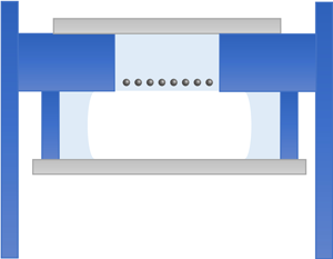
  $0.6\;\mathrm{\mu }\textrm{m}$ (Si3). The particle samples were cleaned 8–10 times via centrifugation prior to use to scour off the surfactant in the solution. Then, the cleaned particles were suspended in deionized water to form preparatory samples. The deionized (DI) water was produced using a Synergy UV System from Millipore. The sample cell was made of stainless steel and had a structure similar to that in Zhang et al. (Reference Zhang, Chen, Li, Zhang and Chen2013a). The cell consisted of a solution tank at the bottom and an air tank at the top. The inner diameter of the solution tank was 8.3 mm. The depth of both tanks was 0.8 mm. A preparatory sample was introduced into the solution tank until the sample solution bulged. The extra solution was removed using a glass straw. The opening of the straw was half-immersed at the solution surface. When the extra solution was sucked off by the straw, the possible impurities on the interface were also removed. After the prepared cell was sealed with a coverslip, the sealed cell was placed upside down and left undisturbed for 7–8 h. Then, the particles settled down toward the water–air interface under gravity. The surface tension of the water was sufficiently strong to retain the water on the top side of the cell. A stable particle monolayer stays close to the water–air interface due to the interaction of the image charge of the particles. The separation between the water–air interface and the centres of particles in the monolayer is denoted by z. The experimental system is shown in figure 1(a). A microscope (Olympus X71 with 60× objectives, NA 0.70) and a CCD camera (Prosilica GE1050, 1024 pixels × 1024 pixels, 17 fps) were used to record sequences of images of the particles in the monolayer (figure 1b). Each sequence comprised 500 frames. The image resolution of the camera was 0.09 μm pix−1. The closest particles in adjacent frames were identified as the same particle. The particle trajectories
  $\boldsymbol{s}(t)$ were obtained using our homemade particle tracking program.

Figure 1. Schematic view of the experiment. (a) Schematic view of the system. (b) Optical microscope image of silica particles (a = 1.57 μm) suspended near a water–air interface at an area fraction of  $n = 0.04$. (c) The definitions of
  $\Delta {s_{||}}$,
  $\Delta {s_ \bot }$ and
  $\Delta {\boldsymbol{s}_i}(\tau )$.
3. Results
The single-particle self-diffusion coefficient  ${D_s}(n)$ can be obtained from the mean square particle displacement
  $\langle \Delta \boldsymbol{\boldsymbol{\mathsf{S}}_i^2(\tau )\rangle = 4{D_s}(n)\tau}$, where
  $\Delta {\boldsymbol{\boldsymbol{\mathsf{S}}_i}(\tau ) = {\boldsymbol{\boldsymbol{\mathsf{S}}_i}(t + \tau ) - {\boldsymbol{\boldsymbol{\mathsf{S}}_i}(t)}}}$, as shown in figure 1(c). Here,
  $\tau $ is the lag time, and n is the area fraction of the particles. Figure 2(a) shows the normalized curves of
  ${D_s}(n)/{D_0}$ as functions of the particle concentration n for the three samples, where
  ${D_0}$ is the diffusion coefficient for a single particle in the bulk water,
  ${D_0} = {k_B}T/6\pi {\eta ^{(b)}}a$. The value for each data point in figure 2(a) was obtained by averaging more than
  ${10^6}$ particles. The solid lines in figure 2(a) illustrate the results of fitting the data to
  ${D_s}(n)/{D_0} = \alpha (1 - \beta n - \gamma n^2)$ (Chen & Tong Reference Chen and Tong2008). When
  $n \to 0$,
  ${D_s}(0)/{D_0} = \alpha $, where
  ${D_s}(0)$ is the single-particle diffusion coefficient in the monolayer in the dilute limit. The fitted values of the parameters
  $\alpha $,
  $\beta $ and
  $\gamma $ for the three samples are given in table 1. As seen from this table, a larger particle size corresponds to a larger value of
  $\alpha $ and a smaller value of
  $\beta $. Here, the value of the parameter
  $\alpha $ reflects the strength of the viscosity experienced by a single particle in the local environment in the dilute solution limit. A large
  $\alpha $ implies a low viscosity (Zhang et al. Reference Zhang, Chen, Li, Zhang and Chen2013a). The value of the parameter
  $\beta $ represents the strength of the effective hydrodynamic interactions between two particles, excluding the effects of the local environment. A large
  $\beta $ reflects strong hydrodynamic interactions. The value of the parameter
  $\gamma $ represents the strength of the many-body effect among the particles in the monolayer.

Figure 2. (a) Normalized self-diffusion coefficients of a single particle. The normalized self-diffusion coefficient  ${D_s}(n)/{D_0}$ is plotted as a function of the area fraction n for samples Si1, Si2 and Si3. The solid lines represent the second-order polynomial fits to the formula
  ${D_s}(n)/{D_0} = \alpha (1 - \beta n - \gamma {n^2})$ for each sample. (b) The dependence of the Saffman length
  ${\lambda _s}$ of monolayers on the area fraction n for each sample.
Table 1. Parameters of the three samples.

The separation z is calculated according to (3.1) (Wang et al. Reference Wang, Prabhakar and Sevick2009, Reference Wang, Prabhakar, Gao and Sevick2011b):
 \begin{equation}\frac{{{D_s}(0)}}{{{D_0}}} = 1 + \frac{3}{{16}}\left( {\frac{{2{\eta^{(b)}} - 3{\eta^{(a)}}}}{{{\eta^{(b)}} + {\eta^{(a)}}}}} \right)\left( {\frac{a}{z}} \right),\end{equation}
where  ${\eta ^{(b)}}$ is the viscosity of the bulk water,
  ${\eta ^{(a)}}$ is the viscosity of the air and z is the separation between the particle centre and the liquid interface. The calculated values of z are shown in table 1. It should be noted that the thermal motion of the particles prevents them from staying at a fixed location, and rather causes them to sway around their equilibrium positions, while their vertical positions follow a Boltzmann distribution. The measured value of z presented here is an average one, with a fluctuation width
  $\Delta z$ in the order of
  ${k_B}T/\Delta mg$, where
  $\Delta m$ is the difference of the mass between the particle and a water sphere with the same size. This is true for a 1 μm radius silica particle,
  $\Delta z\sim 0.1\;{\rm \mu} \textrm{m}$, for example. All our measurements are the results of HIs averaged in the water film with a thickness of
  ${\sim} \Delta z$. As shown in table 1, a large
  $\alpha $ corresponds to a small separation
  $z/a$, which suggests that the local viscosity is higher when the particle monolayer in the water is farther from the water–air interface.
The water–air interface is perfectly slipping, incapable of supporting a shear stress. Such a slip boundary corresponds to a decreased particle friction (increased mobility) and decreased energy dissipation. Intuitively, the closer a Brownian particle is to the water–air interface, the less surrounding water can be driven by the particle's moving, because the water film between the particle and the interface is thinner. The particle will thus feel less viscosity when approaching the interface, unlike that in the bulk of the water. From (3.1), we can know that for a particle that is far away from the water–air interface, the particle's friction is increased with respect to its bulk value, and the diffusion constant is decreased, so the value of the measured diffuse constant tends to its bulk values.
According to the work of Sickert, Rondelez & Stone (Reference Sickert, Rondelez and Stone2007) and Fischer, Dhar & Heinig (Reference Fischer, Dhar and Heinig2006), the single-particle diffusion coefficient can be written as
 \begin{equation}{D_s}(n) \cong \frac{{{k_B}T}}{{{\kappa ^{(0)}}{\eta ^{(b)}}a + {\kappa ^{(1)}}{\eta ^{(s1)}}(n)}},\end{equation}
where  ${k_B}$ is the Boltzmann constant and
  ${\eta ^{(s1)}}(n)$ is the n-dependent surface viscosity of the particle monolayer. Equation (3.2) indicates that the friction of a particle experienced in a monolayer (or a film) comes from two terms:
  ${\kappa ^{(0)}}{\eta ^{(b)}}a$ and
  ${\kappa ^{(1)}}{\eta ^{(s1)}}$. The first term represents the friction due to the viscosity experienced by the particle in its local environment, where
  ${\eta ^{(b)}}$ is the viscosity of the bulk of fluid and
  ${\kappa ^{(0)}}$ is related to the position of the monolayer. The second term represents the friction coming from the monolayer (or film) itself, which is a function of the area fraction n. The dimensionless coefficients
  ${\kappa ^{(0)}}$ and
  ${\kappa ^{(1)}}$, which are the functions of z, can be calculated by following equations (Fischer et al. Reference Fischer, Dhar and Heinig2006),
 \begin{gather}{\kappa ^{(0)}} \approx 6\pi \sqrt {\tanh \left[ {\frac{{32(z/a + 1)}}{{9{\pi^2}}}} \right]} ,\end{gather}
 \begin{gather}{\kappa ^{(1)}} \approx{-} 4 \times \ln \left( {\frac{2}{\pi }\arctan \left( {\frac{2}{3}} \right)} \right)\frac{{{{(3a)}^{3/2}}}}{{{{(z + 2a)}^{3/2}}}}\quad (z \ge a).\end{gather}
The calculated values of  ${\kappa ^{(0)}}$ and
  ${\kappa ^{(1)}}$ for the three samples are listed in table 1. More details about the method to obtain the values of
  ${\kappa ^{(0)}}$ and
  ${\kappa ^{(1)}}$ are presented in the supplementary material available at https://doi.org/10.1017/jfm.2020.693. Given the results of
  ${D_s}(n)$, the surface viscosity
  ${\eta ^{(s1)}}$ of the monolayers can be estimated by (3.2). The Saffman length
  ${\lambda _s}$ can be obtained by
  ${\lambda _s} = {\eta ^{(s1)}}/{\eta ^{(b)}}$ (Saffman & Delbrück Reference Saffman and Delbrück1975; Saffman Reference Saffman1976). The curves of
  ${\lambda _s}$ vs. n are shown in figure 2(b), which indicates that
  ${\lambda _s}$ increases with n monotonically.
The correlated diffusion reflects the response function of the HIs between two particles (Crocker et al. Reference Crocker, Valentine, Weeks, Gisler, Kaplan, Yodh and Weitz2000; Gardel, Valentine & Weitz Reference Gardel, Valentine and Weitz2005; Prasad et al. Reference Prasad, Koehler and Weeks2006). In terms of the particle displacement, the correlated diffusion coefficient is defined as
 \begin{equation}{D_{||, \bot }}(r) = \frac{{{{\langle \Delta s_{||, \bot }^i(t,\tau )\Delta s_{||, \bot }^j(t,\tau )\delta (r - {R^{i,j}}(t))\rangle }_{i \ne j}}}}{{2\tau }}.\end{equation}
Here,  $\Delta s_{||, \bot }^i$ is the displacement of the
  $i\textrm{th}$ particle in the longitudinal
  $(||)$ or transverse
  $( \bot )$ direction during a time interval
  $\tau $, as shown in figure 1(c). The longitudinal displacement
  $\Delta {s_{||}}$ and transverse displacement
  $\Delta {s_ \bot }$ are the components of
  $\Delta {\boldsymbol{s}_i}(\tau )$ that are parallel and perpendicular, respectively, to the line connecting the centres of two particles i and j. The average
  ${\langle \rangle _{i \ne j}}$ is taken over all pairs consisting of the
  $i\textrm{th}$ and
  $j\textrm{th}$ particles with a separation distance r for
  $i \ne j$. The correlated diffusion coefficients
  ${D_{||, \bot }}(r)$ for sample Si1 are plotted in figure 3(a,b), where the results are normalized with respect to the single-particle diffusion
  ${D_s}(n)$ to eliminate the effects of the local viscosity. In figure 3(a,b), from bottom to top, the area fraction n varies from 0.03 to 0.59, and the black squares and green crosses correspond to the smallest and largest n values, respectively. The curves of
  ${D_{||, \bot }}(r)$ for samples Si2 and Si3 are plotted in figures 3(c,d) and 3(e,f), and exhibit behaviours similar to those of
  ${D_{||\bot }}(r)$ for sample Si1.

Figure 3. Measured correlated diffusion coefficients  ${D_{||}}/{D_s}(n)$ (a) and
  ${D_ \bot }/{D_s}(n)$ (b) as a function of the distance
  $r/(2a)$ for sample Si1; (c and d) for sample Si2; (e and f) for sample Si3. The different symbols represent measurements at different area fractions n. The highest n is labelled in each figure. The dashed lines corresponding to
  ${\sim} 1/r$ (a) and
  ${\sim} 1/{r^2}$ (b) are plotted for reference.
Curves of  ${D_{||\bot }}(r)$ in figure 3(a–f) collapse to a single master curve
  ${\tilde{D}_{||, \bot }}({R_{||, \bot }})$ for each direction when an effective diffusion coefficient
  $D_s^m$ and adjustable parameters
  ${\chi _{||, \bot }}$ are used as the scaling factors in vertical and horizontal axis respectively, i.e.
  ${\tilde{D}_{||}} \equiv {D_{||}}/D_s^m$ and
  ${R_{||, \bot }} \equiv r/{\chi _{||, \bot }}$ (see figure 4). The effective diffusion coefficient
  $D_s^m$ is obtained by the single-particle diffusion coefficient
  ${D_s}(n)$ in the following method. As shown in (3.2), the retardation experienced by a Brownian particle involves two factors: the local viscosity experienced by the particle in the dilute limit
  ${\kappa ^{(0)}}{\eta ^{(b)}}a$ and the many-body effect of the particles
  ${\kappa ^{(1)}}{\eta ^{(s)}}$ in the particle monolayer. Based on (3.2), two effective diffusion coefficients can be defined by
  ${D_s}(0) \equiv {k_B}T/{\kappa ^{(0)}}{\eta ^{(b)}}a$ and
  $D_s^m(n )\equiv {k_B}T/{\kappa ^{(1)}}{\eta ^{(s1)}}$. Hence, (3.2) can be rewritten as
 \begin{equation}\frac{1}{{{D_s}(n)}} = \frac{1}{{{D_s}(0)}} + \frac{1}{{D_s^m(n)}}.\end{equation}
Here,  ${D_s}(0)$ is the diffusion coefficient of a single particle in the monolayer in the dilute limit
  $(n \to 0)$, which can be obtained from figure 2(a), and
  $D_s^m(n)$ is a function of n because the viscosity
  ${\eta ^{(s1)}}$ stems from the HIs between particles in the monolayer. Since the measured correlated diffusion coefficients
  ${D_{||,\; \bot }}(r)$ describe the HIs between particles,
  $D_s^m(n)$ is a more suitable scaling factor than
  ${D_s}(n)$ for this scenario.

Figure 4. Scaled correlated diffusion coefficients  ${\tilde{D}_{||}}({R_{||}})$ (a) and
  ${\tilde{D}_ \bot }({R_ \bot })$ (b) for sample Si1; (c and d) for sample Si2; (e and f) for sample Si3. The symbols used are same as in figure 3.
The scaling factors  ${\chi _{||, \bot }}$, which are the functions of n, can be regarded as characteristic lengths of the particle monolayer. Based on the concept of the Saffman length, the values of
  ${\chi _{||, \bot }}(n)$ are determined by the ratio of the surface viscosity of the monolayer and the bulk viscosity of water (Saffman & Delbrück Reference Saffman and Delbrück1975). When
  ${\chi _{||}}(n)$ obtained in figure 4(a,c,e) are regarded as
 \begin{equation}{\chi _{||}} = \eta _{||}^{(s2)}/{\eta ^{(b)}},\end{equation}
the surface viscosity  $\eta _{||}^{(s2)}$ of the monolayer can be estimated from the value of
  ${\chi _{||}}$. The comparison between such
  $\eta _{||}^{(s2)}$ and
  ${\eta ^{(s1)}}$ is plotted in figure 5(a), which reads that
  $\eta _{||}^{(s2)}$ and
  ${\eta ^{(s1)}}$ agree with each other. The values of
  $\eta _{||}^{(s2)}$ and
  ${\eta ^{(s1)}}$, which are obtained in one-particle and two-particle measurements respectively, should agree with each other for the same homogeneous monolayer (Prasad et al. Reference Prasad, Koehler and Weeks2006; Zhang et al. Reference Zhang, Li, Bohinc, Tong and Chen2013b). Usually, the agreement between
  $\eta _{||}^{(s2)}$ and
  ${\eta ^{(s1)}}$ will be satisfied when n is small. The monolayer can turn into a heterogeneous state with an increase in
  $n.$ Then, there will be a gradual deviation between
  $\eta _{||}^{(s2)}$ and
  ${\eta ^{(s1)}}$ with an increase in n, (Prasad et al. Reference Prasad, Koehler and Weeks2006) as shown in figure 5(a). The results in figure 5(a) suggest that
  ${\chi _{||}}$ is the Saffman length indeed, i.e.
  ${\chi _{||}} = {\lambda _s}$.

Figure 5. (a) Plots of  $\eta _{||}^{(s2)}$ vs.
  ${\eta ^{(s1)}}$ for three samples. (b) Plots of
  $\eta _ \bot ^{(s2)}$ vs.
  ${\eta ^{(s1)}}$ calculated from
  ${\chi _ \bot } = {\lambda _s}$ for three samples. The cyan curves represent fits to
  $\eta _ \bot ^{(s2)}\sim {({\eta ^{(s1)}})^{2/3}}$. (c) Plots of
  $\eta _ \bot ^{(s2)}$ vs.
  ${\eta ^{(s1)}}$ calculated from (3.7). (d) Plots of
  $\eta _ \bot ^{(s2)}$ vs.
  $\eta _{||}^{(s2)}$ from (3.7) for three samples. The navy blue line in (a,c,d) is shown for reference, and the slope of the line is 1.0.
However, we found that  ${\chi _ \bot }(n)$ obtained in figure 4(b,d,f) cannot be regarded as the Saffman length
  ${\lambda _s}$. If
  ${\chi _ \bot }(n) = {\lambda _s}$ was regarded, the values of
  $\eta _ \bot ^{(s2)}$ estimated from
  ${\chi _ \bot }(n) = \eta _ \bot ^{(s2)}/{\eta ^{(b)}}$ would disagree with the values of
  ${\eta ^{(s1)}}$. The comparison between such
  $\eta _ \bot ^{(s2)}$ and
  ${\eta ^{(s1)}}$ is plotted in figure 5(b), indicating that the viscosity
  $\eta _ \bot ^{(s2)}$ obtained from
  ${\chi _ \bot } = {\lambda _s}$ follows the power-law relationship
  $\eta _ \bot ^{(s2)} \sim {({\eta ^{(s1)}})^{2/3}}$. Considering this power-law relationship, the dependence of the scaling length
  ${\chi _ \bot }$ on the Saffman length
  ${\lambda _s} = \eta _ \bot ^{(s2)}/{\eta ^{(b)}}$ should be expressed as
 \begin{equation}{\chi _ \bot } = \frac{1}{2}a{\left( {\frac{{{\lambda_s}}}{a}} \right)^{2/3}},\end{equation}
for  $\eta _ \bot ^{(s2)} = {\eta ^{(s1)}}$ to be satisfied. The viscosity
  $\eta _ \bot ^{(s2)}$ that is obtained using (3.8) is plotted against
  ${\eta ^{(s1)}}$ in figure 5(c). Once again, the values of
  ${\eta ^{(s1)}}$ and
  $\eta _ \bot ^{(s2)}$ agree with each other when n is small. The comparison between the viscosity
  $\eta _{||}^{(s2)}$ and
  $\eta _ \bot ^{(s2)}$ is plotted in figure 5(d), which shows
  $\eta _{||}^{(s2)} = \eta _ \bot ^{(s2)}$ all the time.
It should be noted that there exist sets of values of  ${\chi _{||, \bot }}$ and their multiples such that all of these values can make
  ${\tilde{D}_{||, \bot }}$ collapse to a single curve. However, there is only one special pair of
  ${\chi _{||, \bot }}$ values for which the calculated viscosity
  ${\eta ^{(s2)}} \equiv \eta _{||, \bot }^{(s2)}$ agrees with
  ${\eta ^{(s1)}}$. This constraint allows for one to determine a unique pair of
  ${\chi _{||, \bot }}$ values with which to determine the positions of the master curves of
  ${\tilde{D}_{||, \bot }}$.
The dependence of  ${\eta ^{(s2)}}$ on n is plotted in figure 6, showing that it follows the Krieger–Dougherty equation (Krieger & Dougherty Reference Krieger and Dougherty1959) as follows:
 \begin{equation}{\eta ^{(s2)}} = {\eta ^{(s1)}}(0)\left[ {{{\left( {1 - \frac{n}{{{n_m}}}} \right)}^{ - [\eta ]{n_m}}} - 1} \right],\end{equation}
where  ${\eta ^{(s1)}}(0)$ is a characteristic scale for the surface viscosity, which is affected by the confining boundary. In the above equation,
  ${n_m} \cong 0.84$ is the maximum random packing fraction in two dimensions (Berryman Reference Berryman1983; O'Hern et al. Reference O'Hern, Langer, Liu and Nagel2002), and the intrinsic viscosity
  $[\eta ]$ is the only fitting parameter. The fitted values of the intrinsic viscosity
  $[\eta ]$ are shown in table 1.

Figure 6. The surface viscosities  ${\eta ^{(s2)}}$ as functions of the particle area fraction n. The cyan curves represent fits to the Krieger–Dougherty equation.
In the vicinity of a fluid–fluid interface, the mobility of particles and the hydrodynamic interactions between particles will be different from those in the bulk, which show a complex dependence on the separation z (Jones, Felderhof & Deutch Reference Jones, Felderhof and Deutch1975; Bickel Reference Bickel2007; Wang et al. Reference Wang, Prabhakar and Sevick2009, Reference Wang, Prabhakar, Gao and Sevick2011b). In our experiments,  ${\tilde{D}_{||}}$ and
  ${\tilde{D}_ \bot }$ indeed depend on the separation z. The larger z is, the weaker the influence of the water–air interface. The master curves of
  ${\tilde{D}_{||}}({R_{||}})$ and
  ${\tilde{D}_ \bot }({R_ \bot })$ with different z each degenerate to a single curve when
  ${\tilde{D}_{||}}({R_{||}})$ and
  ${\tilde{D}_ \bot }({R_ \bot })$ are multiplied by a factor of
  ${(z/a)^{2/3}}$ (as shown in figure 7). This degeneracy of
  ${\tilde{D}_{||, \bot }}$ by a factor of
  ${(z/a)^{2/3}}$ at
  $z \gt 0$ indicates that, with the exception of the boundary effect, no dynamic mechanisms are introduced into the system by the water–air interface.

Figure 7. (a) Universal master curve of  ${\tilde{D}_{||}} {(z/a)^{2/3}}$ as a function of
  ${R_{||}}$ for three samples. (b) Universal master curve of
  ${\tilde{D}_ \bot } {(z/a)^{2/3}}$ as a function of
  ${R_ \bot }$ for three samples.
It can be seen from figure 7(b) that the value for Si3 is slightly lower than the other two. This deviation between them looks more obvious in the half-log plot (see supplementary figure S1). We think that such deviation comes from fluctuations in the vertical position of the particles, which will weaken HIs between the particles at given projection distance r. The smaller the mass of the particles, the greater the fluctuations experienced in the vertical position. The correlated diffusion,  ${D_{||\bot }}(r)$, of Sample Si3 was smaller than that of the other two samples. Another feature of such deviation is that a significant deviation appears in a short distance, as the strength of such an influence is supposed to be proportional to
  $\Delta z/r$.
4. Discussion
It should be noted that the screened Coulomb repulsive interaction exists in addition to hydrodynamic interactions between the charged particles immersed in water. However, such a Coulomb interaction is a short-range interaction, which usually occurs in few Debye screening lengths. The samples were left undisturbed for 7–8 h before the measurement. The CO2 resolves in the DI water during this time, which increases the concentration of counterions in the water solution and reduces the Debye screening lengths to the order of 0.1 μm. The measured  ${D_{||, \bot }}(r)$ in a range of 2–30 μm in figure 3 will not be affected by such a short-range interaction. The particles totally immerse in the water and are away from the interface, which excludes the presence of capillary interaction or dipole interaction between the particles. In fact, the hydrodynamic interaction is the only long-range interaction in our system, which corresponds to the behaviours of
  ${D_{||\bot }}(r)$ obtained here.
When  $r \gg {\lambda _s}$, one usually has
  ${D_{||}}(r)\sim 1/r$ and
  ${D_ \bot }(r)\sim 1/{r^2}$ for the monolayer of particles suspended in a liquid. The particles in such a 2-D monolayer cannot conserve momentum, but diffuse momentum into the surrounding fluid, leading to the fact that the r-dependence of
  ${D_{||, \bot }}$ in the monolayer is dominated by the surrounding liquid. In the longitudinal direction, the dependence of
  ${D_{||}}(r)\sim 1/r$ is identical to the longitudinal correlation in an unbounded fluid, caused by 3-D shear stresses, while in the transverse direction, the dependence of
  ${D_ \bot }(r)\sim 1/{r^2}$ arises from 2-D compressive stresses due to the force of effective dipoles. For a particle monolayer located just at the water–air interface (figure 8a), the scaling lengths in the longitudinal and transverse directions are identical (Prasad et al. Reference Prasad, Koehler and Weeks2006; Zhang et al. Reference Zhang, Li, Bohinc, Tong and Chen2013b). In our experiments, however, the monolayer is located a short distance from the water–air interface (figure 8b), and the scaling lengths differ in the two directions. This phenomenon can be attributed to the boundary effect of the water–air interface. Figure 3(a,c,e) shows that
  ${D_{||}}(r)$ decays with r as
  ${\sim} 1/r$ in the longitudinal direction. This results from the HIs response to a 3-D-like shear stress in the bulk water and the thin-film water, which acts as a kind of semi-3-D system due to the momentum conservation in a 3-D liquid (Nägele et al. Reference Nägele, Kellerbauer, Krause and Klein1993; Crocker et al. Reference Crocker, Valentine, Weeks, Gisler, Kaplan, Yodh and Weitz2000; Levine & Lubensky Reference Levine and Lubensky2000; Oppenheimer & Diamant Reference Oppenheimer and Diamant2009, Reference Oppenheimer and Diamant2010). In figure 3(b,d,f),
  ${D_ \bot }(r)$ decays as
  ${\sim} 1/{r^2}$ in the transverse direction, showing behaviour that has been attributed to long-range compression and modelled as interactions of effective mass dipoles (Cui et al. Reference Cui, Diamant, Lin and Rice2004; Shani et al. Reference Shani, Beatus, Bar-Ziv and Tlusty2014). This difference in the variation tendencies of the correlated diffusion coefficients in the longitudinal and transverse directions is universal among colloidal monolayers suspended in fluids (Oppenheimer & Diamant Reference Oppenheimer and Diamant2009, Reference Oppenheimer and Diamant2010).

Figure 8. Two kinds of colloidal systems. (a) The particle monolayer is at the water–air interface. (b) The particle monolayer is near the water–air interface.
In this water–air system, the scaling length is separated into a longitudinal scaling length  ${\lambda _s}$ and a transverse scaling length
  ${\chi _ \bot }$. Such a scaling method for r can also be applied in a similar way to the water–oil system. The relationship between them follows
  $2{\chi _ \bot }/a = {({\lambda _s}/a)^{2/3}}$. This relationship may be understood by comparison with that of the lubrication of a liquid film confined between two solid surfaces. The normal load capacity of the film depends on the form of hydrodynamic action that the film experiences (Hamrock, Schmid & Jacobson Reference Hamrock, Schmid and Jacobson2004). In the case of squeezing action, the normal load capacity is
  ${W_{squeeze}} = (w^{\prime}/{\eta ^{(b)}}{u_{squeeze}}){({h_{squeeze}}/l)^3}$, where
  $w^{\prime}$,
  ${u_{squeeze}}$,
  ${h_{squeeze}}$, and l are the normal load per unit length, squeezing velocity, film thickness and length of the solid surface, respectively. Similarly, the expression for the load capacity for sliding action (Hamrock et al. Reference Hamrock, Schmid and Jacobson2004) is
  ${W_{sliding}} = (w^{\prime}/({\eta ^{(b)}}{u_{sliding}})){({h_{sliding}}/l)^2}$, where
  ${h_{sliding}}$ is the thickness of the liquid film and
  ${u_{sliding}}$ is the sliding velocity. When these two load capacities are comparable (i.e.
  ${W_{squeeze}}\sim {W_{sliding}}$) with
  ${u_{squeeze}} = {u_{sliding}}$, the equation
  ${h_{squeeze}}/l\sim {({h_{sliding}}/l)^{2/3}}$ is obtained, with a functional form similar to that of
  $2{\chi _ \bot }/a = {({\lambda _s}/a)^{2/3}}$. This analogy is based on the recognition that the squeezing and sliding actions for a confined film are equivalent to the compression and shear stress between the particles in a particle monolayer (Oppenheimer & Diamant Reference Oppenheimer and Diamant2009, Reference Oppenheimer and Diamant2010). Thus, the relationship between the two scaling lengths of the particle monolayer has the same form as that of
  ${h_{squeeze}}/l = {({h_{sliding}}/l)^{2/3}}$.
The form of the scaling length  ${\chi _ \bot } = a{({\lambda _s}/a)^{2/3}}/2$ can also be understood by analogy to lubrication theory. The squeezing force between two particles of radius a with a separation distance r in a liquid is
  $f = \xi (r)U$, where U is the velocity at which one particle is approaching the other and
  $\xi (r)$ is the hydrodynamic friction coefficient. When the two particles are suspended in a 3-D liquid with a separation distance
  ${r_{3D}}$, the friction coefficient is
  $\xi ({r_{3D}}) = (3/2)\pi {\eta ^{(b)}}a(a/{r_{3D}})$ (Russel, Saville & Schowalter Reference Russel, Saville and Schowalter1992). In a 2-D system, such as two circular disks of radius a with a separation distance
  ${r_{2D}}$ approaching each other in a thin liquid film (Hamrock et al. Reference Hamrock, Schmid and Jacobson2004), the friction coefficient of the squeezing force is
  $\xi ({r_{2D}}) = (3/2)\pi {\eta _s}{(a/{r_{2D}})^{3/2}}$. Here, the viscosity of the film,
  ${\eta _s}$, is equal to
  ${\eta ^{(b)}}a$. By equating these two kinds of squeezing lubrication forces [i.e.
  $\xi ({r_{2D}}) = \xi ({r_{3D}})$], we find that
  ${r_{2D}} = a{({r_{3D}}/a)^{2/3}}$, which is similar to
  ${\chi _ \bot } = a{({\lambda _s}/a)^{2/3}}/2$.
5. Conclusions
In this work, for a particle monolayer near a water–air interface, the correlated diffusion coefficients of the particles in the longitudinal and transverse directions are presented in the form of normalized functions  ${\tilde{D}_{||, \bot }}({R_{||, \bot }})$. From such correlated diffusion measurements, the longitudinal scaling length is the Saffman length
  ${\lambda _s}$ of the particle monolayer, and the transverse scaling length
  ${\chi _ \bot }$ follows a power-law relationship with
  ${\lambda _s}$, as expressed by
  ${\chi _ \bot } = a{({\lambda _s}/a)^{2/3}}/2$. Using these scaling lengths, the master curves of the correlated diffusion and viscosity of such particle monolayers can be obtained. Studies of the correlated diffusion of a colloidal monolayer near a water–oil interface have been reported previously (Zhang et al. Reference Zhang, Chen, Li, Zhang and Chen2013a). Data collapse into master curves was achieved by a phenomenological scaling method, which does not improve our understanding. Compared with the previous results, the scaling lengths in this work provide a better way to understand the collapse of correlated diffusion curves. Using the scaling method described here, the surface viscosities of monolayers can be calculated correctly. Our experiments provide a set of reliable data that can be used for the further development of theoretical models to study the dynamics of liquids near soft interfaces.
Acknowledgements
This research is supported by the National Natural Science Foundation of China (Grant Nos. 11474054, 11774417 and 11604381), and the Natural Science Foundation of Jiangsu Province (Grant No. BK20160238).
Declaration of interests
The authors report no conflict of interest.
Supplementary material
Supplementary material is available at https://doi.org/10.1017/jfm.2020.693.


