A Numerical Approach to GPS Satellite Perturbed Orbit Computation

Stelian Cojocaru

doi:10.1017/S0373463307004377

A Numerical Approach to GPS Satellite Perturbed Orbit Computation

Published online by Cambridge University Press: 09 August 2007

Stelian Cojocaru

Show author details

Stelian Cojocaru: Affiliation:
(NATO Maritime Component Command, Naples) (Email: cojocarus@yahoo.com)

Article contents

Abstract
INTRODUCTION
REPRESENTATION OF THE GPS SATELLITE PERTURBED MOTION
PERTURBING POTENTIALS
NUMERICAL INTEGRATION
CONCLUSIONS
Footnotes
References

Rights & Permissions

Abstract

This paper proposes a numerical algorithm designed to integrate the GPS satellite perturbed orbit. The numerical solution is applied to integrate the differential equation of perturbed motion that frames the significant perturbing accelerations. Perturbing potentials are given and the corresponding accelerations in Cartesian coordinates are subsequently deduced. The C++ program that implements a fourth-order Runge-Kutta algorithm is described and comment is made on the perturbed orbit integration results. The paper offers a set of conclusions that will hopefully create a quantitative and qualitative image of GPS orbital perturbations and open a few ways ahead.

Keywords

GPS satellite Osculating elements Numerical integration

Type: Research Article
Information: The Journal of Navigation , Volume 60 , Issue 3 , September 2007 , pp. 483 - 495

DOI: https://doi.org/10.1017/S0373463307004377 [Opens in a new window]
Copyright: Copyright © The Royal Institute of Navigation 2007

1. INTRODUCTION

Study of Earth's artificial satellite perturbed motion has, historically speaking, raised difficult, as yet unsolved problems. Closely connected to the three-body problem, it permits only non-exact, partial approaches. Both analytical and numerical solutions have their strengths and weaknesses, as numerous studies have unveiled over the years. In principle, the analytical orbit integration attempts to find algebraic expressions for all accelerations acting upon the satellite and to integrate them in a close form. To perform that, a parameterization has to be made by means of Keplerian orbital elements. Usually, these parameters are the coefficients of the Earth's gravitational potential and/or parameters of other disturbing potentials. A special difficulty appears in the case of discontinuous, non-conservative force fields, e.g. the Sun's radiation pressure. In the numerical orbit integration, a direct, explicit computation of all perturbing accelerations is performed and then, starting from known initial (Cauchy) conditions, a step-by-step direct integration of accelerations is made.

2. REPRESENTATION OF THE GPS SATELLITE PERTURBED MOTION

In the absence of any perturbing influence, the equation of motion of a unit-mass probe particleFootnote ¹ around a central attracting body has the well-known representation (Brower and Clemence Reference Brouwer and Clemence1961, p. 11, Zhang et al. Reference Zhang, Zhang, Grenfell and Deakin2006, p. 295):

(1)

$\ddot{\vec{r}} \equals \minus \mu {{\vec{r}} \over {r^{\setnum{3}} }}\comma$

derived from Newton's universal attraction law.

When projected on the Cartesian reference system, Equation (1) becomes:

(2)

$\ddot{{\rm x}} \equals \minus \rmmu {{\rm x} \over {{\rm r}^{\rm \setnum{3}} }}\semi \quad \ddot{{\rm y}} \equals \minus \rmmu {{\rm y} \over {{\rm r}^{\rm \setnum{3}} }}{\rm \semi }\quad \ddot{{\rm z}} \equals \minus \rmmu {{\rm z} \over {{\rm r}^{\rm \setnum{3}} }}{\rm \comma}$

where μ =M⋅G, the product between the Earth's mass (M) and the universal gravitational constant (G), is the Earth's gravitational parameter. Equation (1) clearly indicates the co-linearity of the satellite's geocentric position vector $\vec{{\rm r}}$ and its acceleration vector $\ddot{\vec{{\rm r}}}$ . When analytically integrated, the system (1) provides 6 integration constants, generally recognized as the Keplerian elements of an un-perturbed GPS satellite orbit, whose significance was extensively explained in the satellite-related literature.

The Keplerian orbit of a satellite is purely a theoretical notion. The homogeneous, 2nd order differential Equation (1) describes the ideal satellite's elliptic motion. To describe the real, perturbed motion of a GPS satellite, one has to add all known perturbing accelerations in the right member of the system (1), obtaining the un-homogeneous, 2nd order differential equation of the perturbed motion of a GPS satellite:

(3)

$\hskip-2\ddot{\hskip2\vec{{\rm r}}} \equals \minus \rmmu {{\vec{{\rm r}}} \over {{\rm r}^{\setnum{3}} }} \plus {\rm d}\hskip-2 \ddot {\hskip2\vec{\rm r}}}$

and subsequently on the Cartesian axes:

(4)

$\ddot{{\rm x}} \equals \minus \rmmu {{\rm x} \over {{\rm r}^{\setnum{3}} }} \plus {\rm d}\ddot{\rm x}\semi } \quad \ddot{{\rm y}} \equals \minus \rmmu {{\rm y} \over {{\rm r}^{\setnum{3}} }} \plus {\rm d}\ddot{\rm y}}\semi \quad \ddot{{\rm z}} \equals \minus \rmmu {{\rm z} \over {{\rm r}^{\setnum{3}} }} \plus {\rm d}\ddot{\rm z}\comma}$

where ${\rm d}\hskip-2 \ddot{\hskip2\vec{\rm r}}}$ represents the sum of all known perturbing accelerations.

When analytically approached, the solution of the homogeneous part of system (3) consists in a set of six constants:

(5)

${\rm p}_{{\rm i}_{{{\rm \setnum{0}}_{{\lpar {\rm i} \equals \setnum{1} \ldots \setnum{6}\rpar }} }} } {\rm \equals \{ a\comma }\,{\rm e\comma }\,{\rm i\comma }\,\rmomega {\rm \comma }\,\rmOmega \comma \,{\rm M\} \comma}$

the Keplerian elements, shaping a time-invariable Keplerian orbit of the GPS satellite at a reference epoch t ₀, as represented in Figure 1 where:

• a, semi-major axis of the orbital ellipsis;
• e, eccentricity of the orbital ellipsis;
• i, inclination of the orbital plan on the Equator plane;
• Ω, longitude (or right ascension) of the ascending node of the orbit;
• ω, argument of the perigee;
• ν, true anomaly, which may replace M (mean anomaly), as the latter has no geometrical significance. Sometimes t₀ (time of satellite's passage through the perigee) is used instead of ν and M.

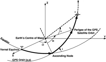
Figure 1. GPS satellite orbit representation.

Any perturbing acceleration added in the right member of Equation (3) will produce temporal variations ( $\dot{{\rm p}}_{i_{\setnum{0}}}$ ) of the orbital parameters. At a later epoch t, the parameters p _i will describe an osculating orbit, defined by:

(6)

$p_{i} \equals {\rm p}_{{\rm i}_{\setnum{0}} } \plus \dot{p}_{i_{\setnum{0}} } \lpar {\rm t} \minus {\rm t}_{\setnum{0}} \rpar \comma _{\;\lsqb {\rm i} \equals \setnum{1} \, \ldots \, \setnum{6}\rsqb}$

As a consequence of (6), the position $\vec{{\rm r}}$ and speed $\hskip-2\dot{\hskip2\vec{{\rm r}}}$ of a GPS satellite in a perturbed motion could be written as:

(7)

$\eqalign{\tab \vec{{\rm r}} \equals \vec{{\rm r}}\lpar {\rm t}\comma {\rm p}_{\rm i} \lpar {\rm t}\rpar \rpar \cr \tab \hskip-2\dot{\hskip2\vec{{\rm r}}} \equals \hskip-2\dot{\hskip2\vec{{\rm r}}}\lpar {\rm t}\comma {\rm p}_{{\rm i}} \lpar {\rm t}\rpar \rpar \cr}$

Deriving (7) by taking into account (3), will result in:

(8)

$\eqalign{\tab \hskip-2\dot{\hskip2\vec{{\rm r}}} \equals {{\partial \vec{{\rm r}}} \over {\partial {\rm t}}} \plus \sum\limits_{{\rm i} \equals \setnum{1}}^{\setnum{6}} {\left( {{{\partial \vec{{\rm r}}} \over {\partial {\rm p}_{\rm i} }} \cdot {{{\rm dp}_{\rm i} } \over {{\rm dt}}}} \right)} \cr \tab \ddot{\vec{{\rm r}}} \equals {{\partial \hskip-2\dot{\hskip2\vec{{\rm r}}}} \over {\partial {\rm t}}} \plus \sum\limits_{{\rm i} \equals \setnum{1}}^{\setnum{6}} {\left( {{{\partial \hskip-2\dot{\hskip2\vec{{\rm r}}}} \over {\partial {\rm p}_{\rm i} }} \cdot {{{\rm dp}_{\rm i} } \over {{\rm dt}}}} \right) \equals \minus \rmmu {{\vec{{\rm r}}} \over {{\rm r}^{\rm \setnum{3}} }} \plus {\rm d}\hskip-2\ddot{\hskip2\vec{\rm r}}}} \cr}$

Vector Equations (8) correspond to 6 scalar equations, which can be put in a simplified vector representation (cf. Hofmann-Wellenhof, Reference Hofmann-Wellenhof, Lichtenegger and Collins1993):

(9)

$\vec{{\rm A}} \cdot \vec{{\rm u}} \equals \vec{\ell }\comma$

where:

(10)

$\left\{ \eqalign{\tab \vec{{\rm A}} \equals \left[ {\matrix{{\displaystyle{{\partial \vec{{\rm r}}} \over {\partial {\rm a}}}} \hfill \tab \displaystyle{{{\partial \vec{{\rm r}}} \over {\partial {\rm e}}}} \hfill \tab {\displaystyle{{\partial \vec{{\rm r}}} \over {\partial {\rm i}}}} \hfill \tab {\displaystyle{{\partial \vec{{\rm r}}} \over {\partial \rmOmega }}} \hfill \tab {\displaystyle{{\partial \vec{{\rm r}}} \over {\partial \rmomega }}} \hfill \tab {\displaystyle{{\partial \vec{{\rm r}}} \over {\partial {\rm M}}}} \hfill \cr {\displaystyle{{\partial \hskip-2\dot{\hskip2\vec{{\rm r}}}} \over {\partial {\rm a}}}} \hfill \tab {\displaystyle{{\partial \hskip-2\dot{\hskip2\vec{{\rm r}}}} \over {\partial {\rm e}}}} \hfill \tab {\displaystyle{{\partial \hskip-2\dot{\hskip2\vec{{\rm r}}}} \over {\partial {\rm i}}}} \hfill \tab {\displaystyle{{\partial \hskip-2\dot{\hskip2\vec{{\rm r}}}} \over {\partial \rmOmega }}} \hfill \tab {\displaystyle{{\partial \hskip-2\dot{\hskip2\vec{{\rm r}}}} \over {\partial \rmomega }}} \hfill \tab {\displaystyle{{\partial \hskip-2\dot{\hskip2\vec{{\rm r}}}} \over {\partial {\rm M}}}} \hfill \cr} } \right] \cr \tab \vec{{\rm u}} \equals \left[ {\matrix{ {\dot{{\rm a}}} \hfill \tab {\dot{{\rm e}}} \hfill \tab {\dot{{\rm i}}} \hfill \tab {\dot{\rmOmega }} \hfill \tab {\dot{\rmomega }} \hfill \tab {\dot{{\rm M}}} \hfill \cr} } \right]^{\rm T} \cr \tab \vec{\ell } \equals \left[ {\matrix{ {\vec{0}} \cr {{\rm d}\hskip-2\ddot{\hskip2\vec{\rm r}}}} \cr} } \right] }\right.}$

• $\vec{{\rm A}}$ is the Jacobian matrix of the orbital elements (5) and position elements (7), comprising 36 elements (6 lines×6 columns) when expressed in Cartesian coordinates;
• $\vec{\ell}$ is the matrix of perturbing accelerations;
• $\vec{{\rm u}}$ is the matrix of the 6 osculating elements' variations under the influence of the perturbing accelerations.

Inversion of (9) will result in Lagrange Planetary Equations (LPE), which contain perturbing potentials Footnote ² (ℜ) instead of perturbing accelerations ( $\ddot{\vec{{\rm r}}}$ ):

(11)

$\nabla \Re \equals {\rm d}\hskip-2 \ddot{\hskip2\vec{\rm r}}\comma }$

where ▽ is the Hamilton operator.

3. PERTURBING POTENTIALS

There are a number of small perturbing influences acting against GPS satellites, significantly smaller than the central attracting acceleration, which produce deviations of the GPS satellite from its Keplerian orbit. The perturbing influences, shown in Table 1, are significant in GPS satellite dynamics.

Table 1. Perturbing influences on GPS satellite motion.

¹ In GPS case, the atmospheric drag is negligible due to the high flight altitude of the GPS satellites.

To evaluate the osculating elements (matrix $\vec{{\rm u}}$ ), the system (10) may be approached either analytically, using the first order perturbation theory, or numerically, using a numerical integrator. In the analytical solution, all perturbing potentials (matrix $\vec{\ell}$ applied to relation 11) must be expressed in terms of osculating elements (5). However, the numerical solution intended in this paper requires all perturbing accelerations to be expressed in Cartesian elements.

The magnitude of the perturbing acceleration depends on both the natural phenomenon which produces it and the average orbital elements of the satellite. Nevertheless, the most important influence on GPS satellite dynamics is represented by the non-central nature of the Earth's gravitational field, namely the deviation of the Earth's natural shape from the spherical symmetry. In general terms, the effects of any perturbing acceleration on GPS osculating elements might be:

• secular: the effect of the perturbation on an osculating element is timely cumulative;
• periodic: the effect of the perturbation on an osculating element alternates in time.

The spectrum of perturbations in GPS orbital elements due to the non-central gravitational field of the Earth are given in Table 2.

Table 2. Types of perturbations of GPS osculating elements.

Further, a general overview of the perturbation magnitude produced in the GPS satellite osculating position ( $\vec{{\rm r}}$ ) is given in Table 3 (cf. Seeber Reference Seeber1993, p. 97).

Table 3. Generic magnitudes of GPS satellite osculating position.

Perturbing potentials with relevance to this study are those produced by the non-central geopotential, Moon-Sun attraction and the Sun's radiation pressure. The perturbing potential created by the non-central part of the Earth's gravitational field derives from the general formula of the Earth's geopotential, in polar coordinates, given by Heiskanen and Moritz Reference Heiskanen and Moritz1967, p. 342:

(12)

${\rm V} \equals {\textstyle{\mu \over {\rm r}}}\left\{ {1 \minus \sum\limits_{\ell \equals \setnum{2}}^{\infty } {\left( {{\textstyle{{{\rm a}_{\rm e} } \over {\rm r}}}} \right)^{\ell } {\rm J}_{\ell } {\rm P}_{\ell } \lpar\hskip-1 \sin\hskip-1 \rmphiv \rpar \minus \sum\limits_{\ell \equals \setnum{2}}^{\infty } {\sum\limits_{{\rm m} \equals \setnum{1}}^{\ell } {\left( {{\textstyle{{{\rm a}_{\rm e} } \over {\rm r}}}} \right)^{\ell } \left[ {{\rm C}_{\ell {\rm m}} \cos {\rm m}\rmlambda \plus {\rm S}_{\ell {\rm m}} \sin {\rm m}\rmlambda } \right]{\rm P}_{\ell {\rm m}} \lpar \hskip-1\sin\hskip-1 \rmphiv \rpar } } } } \right\}\comma$

where the first term $\left( {{\rmmu \over {\rm r}} \equals {\rm V}_{\setnum{0}} } \right)$ represents the spherical Earth's potential, whose gradient $\left( {{\rm grad}{\rmmu \over {\rm r}} \equals \minus \rmmu {{\vec{{\rm r}}} \over {{\rm r}^{\setnum{3}} }}} \right)$ is the central attractive acceleration in the Keplerian motion, 10⁴ times bigger than the sum of all perturbing accelerations. Perturbing potential will result as the difference:

(13)

$\Re _{\rm T} \equals {\rm V} \minus {\rm V}_{\setnum{0}} \equals \left\{ \hskip-2{\sum\limits_{\ell \equals \setnum{2}}^{\infty } \hskip-1{\left( {{\textstyle{{{\rm a}_{\rm e} } \over {\rm r}}}} \right)^{\ell } {\rm J}_{\ell } {\rm P}_{\ell } \lpar \hskip-1\sin\hskip-1 \rmphiv \rpar \minus \hskip-2\sum\limits_{\ell \equals \setnum{2}}^{\infty } {\sum\limits_{{\rm m} \equals \setnum{1}}^{\ell } {\left( {{\textstyle{{{\rm a}_{\rm e} } \over {\rm r}}}} \right)^{\ell } \lsqb {\rm C}_{\ell {\rm m}} \cos {\rm m}\rmlambda \plus S_{\ell {\rm m}} \sin {\rm m}\rmlambda \rsqb {\rm P}_{\ell {\rm m}} \lpar \hskip-1\sin\hskip-1 \rmphiv \rpar } } } } \hskip-1\right\}$

This difference was first converted in osculating elements by Kaula, Reference Kaula1966, p. 30–37, being useful to develop the analytical integration of EPL. However, to make use of the perturbing potential (13) in the numerical integration process in the final part of our work, we need to transform ℜ_T in Cartesian coordinates. The general relationship between polar and Cartesian coordinates is:

(14)

$\left\{\eqalign{ \tab {\rm r} \equals \sqrt {\left( {{\rm x}^{\rm T} } \right)^{\setnum{2}} \plus \left( {{\rm y}^{\rm T} } \right)^{\setnum{2}} \plus \left( {{\rm z}^{\rm T} } \right)^{\setnum{2}} } \cr \tab \rmtheta \equals {\rm tg}^{ \minus \setnum{1}} \left( {{\textstyle{{\sqrt {\left( {{\rm x}^{\rm T} } \right)^{\setnum{2}} \plus \left( {{\rm y}^{\rm T} } \right)^{\setnum{2}} } } \over {\left( {{\rm z}^{\rm T} } \right)^{\setnum{2}} }}}} \right) \cr \tab \rmlambda \equals {\rm tg}^{ \minus \setnum{1}} \left( {{\textstyle{{{\rm y}^{\rm T} } \over {{\rm x}^{\rm T} }}}} \right)} \right.}$

where θ=90°−φ, the satellite co-latitude has been used. The perturbing acceleration caused by the non-central gravitational field of the Earth is the gradient of the perturbing potential (13) in the terms of Cartesian coordinates (14):

(15)

$\left\{ \eqalign{ \tab {{\partial \Re _{\rm T} } \over {\partial {\rm x}^{\rm T} }} \equals {{\partial \Re } \over {\partial {\rm r}}} \cdot {{\partial {\rm r}} \over {\partial {\rm x}^{\rm T} }} \plus {{\partial \Re } \over {\partial \rmtheta }} \cdot {{\partial \rmtheta } \over {\partial {\rm x}^{\rm T} }} \plus {{\partial \Re } \over {\partial \rmlambda }} \cdot {{\partial \rmlambda } \over {\partial {\rm x}^{\rm T} }} \cr \tab {{\partial \Re _{\rm T} } \over {\partial {\rm y}^{\rm T} }} \equals {{\partial \Re } \over {\partial {\rm r}}} \cdot {{\partial {\rm r}} \over {\partial {\rm y}^{\rm T} }} \plus {{\partial \Re } \over {\partial \rmtheta }} \cdot {{\partial \rmtheta } \over {\partial {\rm y}^{\rm T} }} \plus {{\partial \Re } \over {\partial \rmlambda }} \cdot {{\partial \rmlambda } \over {\partial {\rm y}^{\rm T} }} \cr \tab {{\partial \Re _{\rm T} } \over {\partial {\rm z}^{\rm T} }} \equals {{\partial \Re } \over {\partial {\rm r}}} \cdot {{\partial {\rm r}} \over {\partial {\rm z}^{\rm T} }} \plus {{\partial \Re } \over {\partial \rmtheta }} \cdot {{\partial \rmtheta } \over {\partial {\rm z}^{\rm T} }} \plus {{\partial \Re } \over {\partial \rmlambda }} \cdot {{\partial \rmlambda } \over {\partial {\rm z}^{\rm T} }}} \right.}$

while the partial derivatives of this potential are derived from the Kaula's expression:

(16)

$\left\{\openup3\eqalign{\tab {{\partial \Re _{\rm {T}} } \over {\partial {\rm r}}} \equals \minus {\textstyle{{\rmmu {\rm a}_{{\rm e}} ^{\ell } } \over {{\rm r}^{\ell \plus \setnum{2}} }}}\lpar \ell \plus 1\rpar \left[ {{\rm C}_{\ell {\rm m}} \cos {\rm m}\rmlambda \plus S_{\ell m} \sin {\rm m}\rmlambda } \right] \cdot {\rm P}_{\ell {\rm m}} \left( {\cos \rmtheta } \right)\comma \cr \tab {{\partial \Re _{{\rm T}} } \over {\partial \rmtheta }} \equals {\textstyle{{\rmmu {\rm a}_{{\rm e}} ^{\ell } } \over {{\rm r}^{\ell \plus \setnum{1}} }}}\left[ {{\rm C}_{\ell {\rm m}} \cos {\rm m}\rmlambda \plus {\rm S}_{\ell {\rm m}} \sin {\rm m}\rmlambda } \right] \cdot {\rm P} \prime _{\ell {\rm m}} \left( {\cos \rmtheta } \right) \cdot \sin \rmtheta \comma \cr \tab {{\partial \Re _{{\rm T}} } \over {\partial \rmlambda }} \equals \minus {\textstyle{{\rmmu {\rm a}_{{\rm e}} ^{\ell } } \over {{\rm r}^{\ell \plus \setnum{1}} }}} \cdot {\rm m} \cdot \left[ { \minus {\rm C}_{\ell {\rm m}} \sin {\rm m}\rmlambda \plus {\rm S}_{\ell {\rm m}} \cos {\rm m}\rmlambda } \right] \cdot {\rm P}_{\ell {\rm m}} \left( {\cos \rmtheta } \right)\comma }\right.}$

and the rest of terms in the right side of (15) are computable directly. Using a symbolic processor (Maple V in this case), the perturbing acceleration due to the non-central gravitational field of the Earth, up to the 12th order, in Cartesian coordinates, will result:

(17)

$\openup2\eqalign{{{\partial \Re _{\rm T} } \over {\partial {\rm x}}} \equals \tab \minus {\rm x} \cdot {{\rmmu {\rm a}_{\rm e}^{\setnum{2}} } \over {{\rm r}^{\setnum{5}} }} \cdot \left(\hskip-1 {3{\rm C}_{\setnum{2}} {\rm P}_{\setnum{2}} \plus 4{{\rmmu {\rm a}_{\rm e}^{\setnum{3}} {\rm C}_{\setnum{3}} {\rm P}_{\setnum{3}} } \over {\rm r}} \plus 5{{\rmmu {\rm a}_{\rm e}^{\setnum{4}} {\rm C}_{\setnum{4}} {\rm P}_{\setnum{4}} } \over {{\rm r}^{\setnum{2}} }} \plus 6{{\rmmu {\rm a}_{\rm e}^{\setnum{5}} {\rm C}_{\setnum{5}} {\rm P}_{\setnum{5}} } \over {{\rm r}^{\setnum{3}} }} \plus 7{{\rmmu {\rm a}_{\rm e}^{\setnum{6}} {\rm C}_{\setnum{6}} {\rm P}_{\setnum{6}} } \over {{\rm r}^{\setnum{4}} }}}\right.\cr \quad\tab {\plus } 8{{\rmmu {\rm a}_{\rm e}^{\setnum{7}} {\rm C}_{\setnum{7}} {\rm P}_{\setnum{7}} } \over {{\rm r}^{\setnum{5}} }} \plus 9{{\rmmu {\rm a}_{\rm e}^{\setnum{8}} {\rm C}_{\setnum{8}} {\rm P}_{\setnum{8}} } \over {{\rm r}^{\setnum{6}} }} \plus 10{{\rmmu {\rm a}_{\rm e}^{\setnum{9}} {\rm C}_{\setnum{9}} {\rm P}_{\setnum{9}} } \over {{\rm r}^{\setnum{7}} }} \plus 11{{\rmmu {\rm a}_{\rm e}^{\setnum{10}} {\rm C}_{\setnum{10}} {\rm P}_{\setnum{10}} } \over {{\rm r}^{\setnum{8}} }} \plus 12{{\rmmu {\rm a}_{\rm e}^{\setnum{11}} {\rm C}_{\setnum{11}} {\rm P}_{\setnum{11}} } \over {{\rm r}^{\setnum{9}} }} \minus \cr \tab \plus \left. {{\rm 13}{{\rmmu {\rm a}_{\rm e}^{\setnum{12}} {\rm C}_{\setnum{12}} {\rm P}_{\setnum{12}} } \over {{\rm r}^{\setnum{10}} }}} \right) \minus {{\rmmu {\rm a}_{\rm e}^{\setnum{2}} {\rm cos}\rmphiv } \over {{\rm r}^{\setnum{3}} }}{\rm \ }\left( {{{{\rm C}_{\setnum{2}} {\rm q}_{\setnum{2}} } \over {{\rm r}^{\setnum{3}} }} \plus {{{\rm a}_{\rm e} {\rm C}_{\setnum{3}} {\rm q}_{\setnum{3}} } \over {{\rm r}^{\setnum{4}} }} \plus {{{\rm a}_{\rm e}^{\setnum{2}} {\rm C}_{\setnum{4}} {\rm q}_{\setnum{4}} } \over {{\rm r}^{\setnum{5}} }} \plus {{{\rm a}_{\rm e}^{\setnum{3}} {\rm C}_{\setnum{5}} {\rm q}_{\setnum{5}} } \over {{\rm r}^{\setnum{6}} }}}\right. \cr \tab {\plus {{{\rm a}_{\rm e}^{\setnum{4}} {\rm C}_{\setnum{6}} {\rm q}_{\setnum{6}} } \over {{\rm r}^{\setnum{7}} }}} \plus {{{\rm a}_{\rm e}^{\setnum{5}} {\rm C}_{\setnum{7}} {\rm q}_{\setnum{7}} } \over {{\rm r}^{\rm \setnum{8}} }} \plus \left. {{{{\rm a}_{\rm e}^{\setnum{6}} {\rm C}_{\setnum{8}} {\rm q}_{\setnum{8}} } \over {{\rm r}^{\setnum{9}} }} \plus {{{\rm a}_{\rm e}^{\setnum{7}} {\rm C}_{\setnum{9}} {\rm q}_{\setnum{9}} } \over {{\rm r}^{\setnum{9}} }} \plus {{{\rm a}_{\rm e}^{\setnum{8}} {\rm C}_{\setnum{10}} {\rm q}_{\setnum{10}} } \over {{\rm r}^{\setnum{11}} }} \plus {{{\rm a}_{\rm e}^{\setnum{9}} {\rm C}_{\setnum{11}} {\rm q}_{\setnum{11}} } \over {{\rm r}^{\setnum{12}} }}}\right. \cr\tab\left. \plus {{{\rm a}_{\rm e}^{\setnum{10}} {\rm C}_{\setnum{12}} {\rm q}_{\setnum{12}} } \over {{\rm r}^{\setnum{13}} }}} \right) \cdot\left( {{{{\rm z} \cdot {\rm x}} \over {\sqrt {1 \minus {\textstyle{{{\rm z}^{\setnum{2}} } \over {{\rm r}^{\setnum{2}} }}}} \cdot {\rm r}^{\setnum{3}} }}} \right)$

and analogous for y and z. The following standard notations have been used:

• C _n is the coefficient of the nth zonal harmonic of the geopotential;
• P _n is the nth order Legendre polynomial;
• q _n is the nth order derivative of P _n with respect to cosφ.

The analogue perturbing potential caused by Moon and Sun's gravitational attraction was treated extensively by Kaula 1962, Giacaglia Reference Giacaglia1973, et al. In Cartesian coordinates, the cumulative effect of the two celestial bodies upon a GPS satellite is approximated by the following potential (Cojocaru Reference Cojocaru and Academiei1999, p. 57):

(18)

$\Re _{{\rm L} \minus {\rm S}} \equals \rmmu \prime \left( {{1 \over {\rmDelta \prime }} \minus {{{\rm xx \prime} \plus {\rm yy\prime} \plus {\rm zz\prime}} \over {{\rm r\prime}^{\setnum{3}} }}} \right) \plus \left( {{1 \over {\rmDelta \Prime }} \minus {{{\rm xx \Prime} \plus {\rm yy \Prime} \plus {\rm zz \Prime}} \over {{\rm r \Prime}^{\setnum{3}} }}} \right)\comma$

in which the distance Earth-Moon (Δ′) and Earth-Sun (Δ″) are separately computed for every integration step.

The perturbing acceleration caused by the direct solar radiation pressure is modelled by the system (after Ferraz-Mello Reference Ferraz-Mello1964 and Kozai Reference Kozai1961):

(19)

$\left\{ \eqalign { \tab \ddot{{\rm x}} \equals \minus \rmpsi \lpar \rmlambda \rpar \cdot {\rm k\prime} \cdot {{\rm S} \over {\rm m}} \cdot {\rm q} \cdot \left( {{{\rm x}^{\rm o} \minus {\rm x}} \over {{\rm x}^{\rm o} }} \right) \cr \tab \ddot{{\rm y}} \equals \minus \rmpsi \lpar \rmlambda \rpar \cdot {\rm k\prime} \cdot {{\rm S} \over {\rm m}} \cdot {\rm q} \cdot \left( {{{\rm y}^{\rm o} \minus {\rm y}} \over {{\rm y}^{\rm o} }} \right) \cr \tab \ddot{{\rm z}} \equals \minus \rmpsi \lpar \rmlambda \rpar \cdot {\rm k\prime} \cdot {{\rm S} \over {\rm m}} \cdot {\rm q} \cdot \left( {{{\rm z}^{\rm o} \minus {\rm z}} \over {{\rm z}^{\rm o} }} \right) }\right.}$

(cf. Cojocaru Reference Cojocaru and Academiei1999, p. 61); where (x,y,z)^o are Sun's rectangular coordinates at the observation epoch; (x,y,z) are the rectangular coordinates of the GPS satellite; ψ(λ) is the shadow functionFootnote ³ (defined by Ferraz-Mello Reference Ferraz-Mello1964); λ is Sun's ecliptic longitude; k′ is the satellite reflectivity constantFootnote ⁴; S and m are the satellite's section and mass respectively, while q is the solar constant/light speed ratioFootnote ⁵.

4. NUMERICAL INTEGRATION

Numerical solution of GPS satellite osculating orbit is based on the direct numerical integration of the un-homogeneous, second order differential equation of the perturbed motion:

(20)

$\left\{ \eqalign{\tab \ddot{x} \equals \minus {\mu \over {r^{\setnum{3}} }}x \plus \left[ {\ddot{x}^{T} \plus \ddot{x}^{M} \plus \ddot{x}^{S} \plus \ddot{x}^{R} } \right] \cr \tab \ddot{y} \equals \minus {\mu \over {r^{\setnum{3}} }}y \plus \left[ {\ddot{y}^{T} \plus \ddot{y}^{M} \plus \ddot{y}^{S} \plus \ddot{y}^{R} } \right] \cr \tab \ddot{z} \equals \minus {\mu \over {r^{\setnum{3}} }}z \plus \left[ {\ddot{z}^{T} \plus \ddot{z}^{M} \plus \ddot{z}^{S} \plus \ddot{z}^{R} } \right] }\right.}$

where T, M, S and R denote the non-central Terestrial/gravitational field of the Earth, Moon and Sun's direct gravitational effect and Radiation pressure (direct effect) of the Sun respectively, whose expressions were deduced already.

The numerical integration of the system (20) will provide Cartesian coordinates of the GPS satellite on its perturbed, osculating orbit, at every integration step. The Cartesian result of the integration algorithm is necessary to obtain the same format with the real, observed GPS ephemerisFootnote ⁶, to open the possibility of evaluating the differences between the observed and computed positions and velocities. The numerical computed variations of GPS osculating elements can be deduced subsequently by simple, reversed transformations (Cartesian to orbital). The resulting diagrams expressively represent temporal variations of GPS satellite osculating elements.

A fourth-order Runge-Kutta algorithm has been chosen to integrate the system (20). Having established the initial conditions in the Cauchy problem, e.g. the initial coordinates (x₀, y₀, z₀) and velocity components ( $\dot{{\rm x}}_{\setnum{0}} \comma \dot{{\rm y}}_{\setnum{0}\comma } \dot{{\rm z}}_{\setnum{0}}$ ), at a reference epochFootnote ⁷, a Keplerian orbit has to be computed as a reference. Subsequently, only small differences from the real, perturbed orbit and the reference (Keplerian) orbit have to be integratedFootnote ⁸. The integration process will result in the increments (Δx, Δy, Δz) which, when added to Keplerian elements, will furnish the real, perturbed orbital elements. To start the integration process, the second order equation (20) is turned into a system of two first-order differential equations:

(21)

$\left\{\eqalign{\tab \dot{{\rm x}}\lpar {\rm t}\rpar \equals \dot{{\rm x}}\lpar {\rm t}_{\setnum{0}} \rpar \plus \int\limits_{{\rm t}_{\setnum{0}} }^{\rm t} {\left[ {\ddot{{\rm x}}^{\rm T} \lpar {\rm t}\rpar \plus \ddot{{\rm x}}^{\rm M} \lpar {\rm t}\rpar \plus \ddot{{\rm x}}^{\rm S} \lpar {\rm t}\rpar \plus \ddot{{\rm x}}^{\rm R} \lpar {\rm t}\rpar \minus {\mu \over {{\rm r}^{\setnum{3}} \lpar {\rm t}\rpar }}{\rm x}\lpar {\rm t}\rpar } \right]{\rm dt}} \cr \tab {\rm x}\lpar {\rm t}\rpar \equals {\rm x}\lpar {\rm t}_{\setnum{0}} \rpar \plus \int\limits_{{\rm t}_{\setnum{0}} }^{\rm t} {\dot{{\rm x}}} \lpar {\rm t}\rpar {\rm dt}\cr \tab \dot{{\rm y}}\lpar {\rm t}\rpar \equals \dot{{\rm y}}\lpar {\rm t}_{\setnum{0}} \rpar \plus \int\limits_{{\rm t}_{\setnum{0}} }^{\rm t} {\left[ {\ddot{{\rm y}}^{\rm T} \lpar {\rm t}\rpar \plus \ddot{{\rm y}}^{\rm M} \lpar {\rm t}\rpar \plus \ddot{{\rm y}}^{\rm S} \lpar {\rm t}\rpar \plus \ddot{{\rm y}}^{\rm R} \lpar {\rm t}\rpar \minus {\mu \over {{\rm r}^{\setnum{3}} \lpar {\rm t}\rpar }}{\rm y}\lpar {\rm t}\rpar } \right]{\rm dt}} \cr \tab {\rm y}\lpar {\rm t}\rpar \equals {\rm y}\lpar {\rm t}_{\setnum{0}} \rpar \plus \int\limits_{{\rm t}_{\setnum{0}} }^{\rm t} {\dot{{\rm y}}} \lpar {\rm t}\rpar {\rm dt}\cr \tab \dot{{\rm z}}\lpar {\rm t}\rpar \equals \dot{{\rm z}}\lpar {\rm t}_{\setnum{0}} \rpar \plus \int\limits_{{\rm t}_{\setnum{0}} }^{\rm t} {\left[ {\ddot{{\rm z}}^{\rm T} \lpar {\rm t}\rpar \plus \ddot{{\rm z}}^{\rm M} \lpar {\rm t}\rpar \plus \ddot{{\rm z}}^{\rm S} \lpar {\rm t}\rpar \plus \ddot{{\rm z}}^{\rm R} \lpar {\rm t}\rpar \minus {\mu \over {{\rm r}^{\setnum{3}} \lpar {\rm t}\rpar }}{\rm z}\lpar {\rm t}\rpar } \right]{\rm dt}} \cr \tab {\rm z}\lpar {\rm t}\rpar \equals {\rm z}\lpar {\rm t}_{\setnum{0}} \rpar \plus \int\limits_{{\rm t}_{\setnum{0}} }^{\rm t} {\dot{{\rm z}}} \lpar {\rm t}\rpar {\rm dt} }\right.}$

If the sum of terms under the integral sign is considered a continuous function f[t₁, t₂], then its derivative will be: $\dot{{\rm f}} \equals {\rm df}\sol {\rm dt}$ . The general solution of the generic differential equation $\dot{{\rm f}} \equals {{{\rm df}} \over {{\rm dt}}} \equals {\rm f\prime}\lpar {\rm f}\lpar {\rm t}\rpar \comma {\rm t}\rpar$ is obtained by giving an initial value to the integration constant, f₁=f(t₁). Having the integration interval [t₁, t₂] divided into n steps, the solution at (i+1)th step will be: f_i+1=f_i+Δf, where the small difference Δf will be computed with the formula (cf. Hofmann-Wellenhof Reference Hofmann-Wellenhof, Lichtenegger and Collins1993):

(22)

$\rmDelta {\rm f} \equals {{\rmDelta {\rm t}} \over 6} \cdot \lpar {\rm k}_{\setnum{1}} \plus 2 \cdot {\rm k}_{\setnum{2}} \plus 2 \cdot {\rm k}_{\setnum{3}} \plus {\rm k}_{\setnum{4}} \rpar$

where:

(23)

$\left\{\eqalign {\tab {\rm k}_{\setnum{1}} \equals {\rm f}\left( {{\rm t}_{\rm i} \comma\ {\rm f}\lpar {\rm t}_{\rm i} \rpar } \right)\comma \cr \tab {\rm k}_{\setnum{2}} \equals {\rm f}\left( {{\rm t}_{\rm i} \plus {\textstyle{{\rmDelta {\rm t}} \over 2}}\comma \ {\rm f}\lpar {\rm t}_{\rm i} \rpar \plus {\textstyle{{{\rm k}_{\setnum{1}} } \over 2}}} \right)\cr \tab {\rm k}_{\setnum{3}} \equals {\rm f}\left( {{\rm t}_{\rm i} \plus {\textstyle{{\rmDelta {\rm t}} \over 2}}\comma \ {\rm f}\lpar {\rm t}_{\rm i} \rpar \plus {\textstyle{{{\rm k}_{\setnum{2}} } \over 2}}} \right)\cr \tab {\rm k}_{\setnum{4}} \equals {\rm f}\left( {{\rm t}_{\rm i} \plus \rmDelta {\rm t}\comma \ {\rm f}\lpar {\rm t}_{\rm i} \rpar \plus {\rm k}_{\setnum{3}} } \right) }\right.}\comma$

thus making it possible to compute the values of the generic function for the subsequent moments/steps: t₁+Δt, t₁+2Δt, t₁+3Δt, etc., where t₁ is already known from initial (Cauchy) conditions.

The analytical data flow is represented in Figure 2. The program that implements the above numerical algorithm, called Inteq.exe, was developed in Borland C++. Separately from the main program there have been developed functions, called at every integration stepFootnote ⁹, that provide Sun and Moon coordinates and perturbing accelerations. The “Accel” routines in Figure 2 are those described by relations (17), (18) and (19). Particularly, “Accel 2” interrogates the function “Lunas” at every integration step to be provided with Sun and Moon coordinates. The executable Inteq.exe is fed with the initial conditionsFootnote ¹⁰, the range of the integration step and provides coordinates (x, y, z) and velocity (v_x, v_y, v_z) at every integration step; they are subsequently re-converted to orbital elements for further analysis. However, satellite coordinates are saved in separate files on the hard drive every 15 minutes, to keep the similitude with the observed ephemeris.

Figure 2. Analytical data flow.

5. CONCLUSIONS

To model the perturbations of osculating elements represents a hugely complex problem and the analytical approach, apart from its difficulty, cannot give an exact solution. The modern GNSS applications require not only precision but also rapidity, especially during real time application. More and more GPS satellite trials, projects, applications etc. require the availability of a separate and independent computed orbit of the satellites involved. The numerical integration method has proved its ability to satisfy all these exigencies and this essay is meant to offer a numerical alternative to achieve this sensitive task.

Clearly, the dominant perturbing force on GPS orbits is due to oblateness of the Earth. The equatorial eccentricity of the Earth produces a torque which rotates the GPS satellite's orbit on equatorial plane, i.e. a regression of the ascending node (dΩ/dt). Also, the oblateness of the Earth produces a movement of perigee, i.e. a motion of the line of apsides (dω/dt) in the sense of a GPS satellite's movement, as its inclination is less than the critical inclination (i≅55°<63·4°). Both of the above mentioned perturbations are secular. The numerical simulation applied for a real GPS satelliteFootnote ¹¹ reveals the same conclusion, as shown in Figure 3. The second harmonic of the geopotential does not produce secular perturbations in the elements a, e and i; the result of the numerical integration reveals the same conclusion in Figure 4.

Figure 3. Secular perturbation of Ω due to the main harmonic (J2) of the geopotential.

Figure 4. Periodic perturbation of a due to the main harmonic (J2) of the geopotential.

Furthermore, integrating Equation (20) with only ( $\ddot{\vec{{\rm r}}}^{{\hskip1\rm M}} \plus \ddot{\vec{{\rm r}}}^{{\hskip1\rm S}}$ ) in the right member, i.e. taking into account only Moon-Sun gravitational perturbing influence upon a GPS satellite, periodic perturbations in a, e, i, Ω and ωFootnote ¹² can be put into evidence; however, a secular component of Ω and ω can be put into evidence, as well – see Figure 5.

Figure 5. Secular perturbation of Ω due to the gravitational attraction of Sun and Moon.

Estimating the effect of solar radiation pressure proved to be a difficult task, due to the complex structure of the GPS spatial platform. Using average parameters, the numerical integration clearly indicates slight periodic perturbations (see Figure 6). For advanced researches, additional accelerations could be added in the right side of equations (cf. Seeber Reference Seeber1993): friction caused by charged particles in the upper atmosphere, thermal radiation of the satellite, shadow boundaries, interaction between the geomagnetic (terrestrial) field and the electromagnetic (satellite) field and interplanetary dust/cosmic wind respectively.

Figure 6. Periodic perturbation of orbital inclination due to the Sun's radiation pressure.

Compared to the analytical method, the numerical algorithms are distinguished by their simplicity and general applicability. Nowadays, having powerful computers at hand, the computational effort does not count anymore. Cowell's method offers a wide flexibility in manoeuvring the perturbing accelerations in the right-hand member of the equations of perturbed motion. Thus, new mathematical models for perturbing accelerations can be experimented. Also, weak mathematical models, e.g. those used for the Sun's radiation pressure, might be optimized by analyzing the differences between the numerical computed ephemeris and the observed ephemeris of a GPS satellite. In this case, the convergence coefficient of the two numerical series can be used as a qualitative indicator of the robustness of the parameters used in the perturbing acceleration mathematical model.

ACKNOWLEDGEMENT

The research described in this paper was supported by the Astronomical Institute of the Romanian Academy.

Footnotes

¹ Dynamically speaking, the mass of a GPS satellite (m) is so small compared to that of the Earth (M), that we may correctly associate the GPS satellite with a probe particle, having its mass equal to unit (m=1), moving in the Earth's gravitational field.

² Also called perturbing force function; it is a scalar whose derivative is the perturbing acceleration.

³ ψ(λ)=1 when the satellite is enlighten by the Sun; ψ(λ)=0 when the satellite is in the Sun's shadow. This particular case takes place two times a year and lasts about one hour.

⁴ k=1·44 for the diffuse illumination.

⁵ q=4·65·10⁵ dyne/cm².

⁶ Cartesian components of position (x,y,z) and speed ( $\dot{x}\comma \dot{y}\comma \dot{z}$ ) every 15 minutes.

⁷ Numerical values extracted from an exact GPS ephemeris.

⁸ This method of orbit determination was put into evidence by Cowell in 1910.

⁹ Choosing the integration step proves to be a sensitive issue; its size must be balanced between large values (recommended to minimize the round-off errors) and small values (recommended to minimize the truncation errors). A value between 1 and 10 seconds proved to be optimal.

¹⁰ Previously interpolated from an observed ephemeris, using a Lagrange polynomial interpolator.

¹¹ An initial epoch was chosen at: 00:00:00, 27-09-1994, for the GPS satellite PRN#4. Cauchy conditions: Xo=2017·873929 km; Yo=−15394·807277 km; Zo=21652·716838 km; Vxo=3·740049 km/s; Vyo=0·911161 km/s; Vzo=0·306443 km/s.

¹² Numerically speaking, variations of ω are very difficult to be highlighted for GPS satellites, as the orbital eccentricity is very small (≅0·003°) and the perigee is, consequently, unstable.

References

REFERENCES

Broucke, R. A. (1994). Numerical integration of periodic orbits in the main problem of artificial satellites. Celestial Mech. and Dyn. Astron., 58, 99–123.CrossRef Google Scholar

Brouwer, D., Clemence, G. M. (1961). Methods of Celestial Mechanics. Academic Press, New York and London.Google Scholar

Cojocaru, S. (1996). Period Changes Of Satellite Circular Motion Due To Odd Zonal Harmonics of Geopotential, Romanian Astronomical Journal, 6, 2, 179–183.Google Scholar

Cojocaru, S. (1999). GPS Satellite Dynamics, Romanian Naval Academy Press (Ed. Academiei, Navale), ISBN 973-979-13-8-7.Google Scholar

Cojocaru, S. (2001). Influence Of The Even Zonal Harmonics Of The Geopotential On GPS Satellite Orbits, Romanian Astronomical Journal, 11, 1, 69–76.Google Scholar

Ferraz-Mello, S. (1964). Sur le problème de la pression de radiation dans la thèorie de satellites artificial. C.R. Acad. Sc., Paris, 285, p.463.Google Scholar

Ferraz-Mello, S. (1973). Analytical Study of the Earth's Shadowing Effects on Satellite Orbits. Celest. Mechanics, 5.Google Scholar

Gaposchkin, G. M. (1973). Smithsonian Standard Earth III. Smithsonian Astrophysical Observatory Special report 353, Cambridge, Mass.Google Scholar

Giacaglia, G. E. O. (1973). Lunar Perturbation on Artificial Satellites of the Earth, SAO Special Report 352.CrossRef Google Scholar

Heiskanen, and Moritz, (1967). Physical Geodesy', Technical University of Graz.CrossRef Google Scholar

Hofmann-Wellenhof, B., Lichtenegger, H., Collins, J. (1993). GPS – Theory and Practice. Second edition, Springer-Verlag, New York.Google Scholar

Kaula, W. M. (1966). Theory of satellite geodesy. Blaisdell Publ.Co., Waltham.Google Scholar

Kovalevsky, J., Mueller, I. I., Kolaczeck, B. (1989). Reference frames in Astronomy and Geophysics. Kluwer Academic Publ., Dordrecht.CrossRef Google Scholar

Kozai, Y. (1961). Effects of Solar Radiation Pressure on the motion of an artificial Satellite, SAO Special Report 56.Google Scholar

Kozai, Y. (1962). Numerical Results from Orbits. Smithsonian Astrophysical Observatory, Special Report 101.Google Scholar

Leick, A. (1995). GPS Satellite Surveying', 2nd Edition, John Wiley & Sons.Google Scholar

Seeber, G. (1993). Satellite Geodesy. W. de Gruyter.Google Scholar

Zhang, J., Zhang, K, Grenfell, R, Deakin, R. (2006). GPS Satellite Velocity and Acceleration Determination using the Broadcast Ephemeris. The Journal of Navigation, 59, 293–305.CrossRef Google Scholar