1. INTRODUCTION
When transmitted from a satellite to a Global Navigation Satellite System (GNSS) receiver, the carrier frequency and code phase of a signal will change due to the Doppler effect. The signal will also be drowned in noise. So, the GNSS receiver has to extract the signal from noise by a correlation method. The purpose of acquisition is to determine the visible satellites, coarse values of Doppler shift and the phase of a Pseudo-Random Noise (PRN) code (Rinder, Reference Rinder2004). Popular estimation algorithms of the phase of the PRN code and a Doppler shift for satellite signals include the Serial Search acquisition Algorithm (SSA), Parallel Code phase search acquisition Algorithm (PCA) and Parallel Frequency space search acquisition Algorithm (PFA) (Thakar and Mewada, Reference Thakar and Mewada2012).
The time needed to acquire a satellite signal is one of the most important parameters for a BeiDou satellite receiver (Xie et al., Reference Xie, Sun, Kang and Qian2017). Most current receivers use fast acquisition algorithms. The traditional fast acquisition algorithms include PCA and PFA. The PCA algorithm, as shown in Figure 1, consists of six steps: the first step is to remove the Doppler shift of the carrier wave; the second step is to perform Fast Fourier Transform (FFT) on the satellite signal after the Doppler shift of the carrier wave is removed; the third step is to perform FFT on the locally generated PRN code sequence and perform complex conjugate processing; the fourth step is to multiply the second and third results; the fifth step is to take the inverse Fourier transform of the outputs of the fourth step and the last step is to compare the peak value of FFT outputs with the acquisition threshold to determine whether the satellite signal has been acquired. The PFA algorithm, as shown in Figure 2, consists of three steps: the first step is to strip away the PRN code; the second step is to estimate the Doppler shift through FFT and the third step is to compare the peak value of FFT outputs with the acquisition threshold to determine whether the satellite signal has been acquired.

Figure 1. PCA algorithm.

Figure 2. PFA algorithm.
Both the PCA algorithm and the PFA algorithm convert the signal from time-domain to frequency-domain using FFT. PCA does a parallel search of the PRN code and a serial search of the frequency or Doppler shift (Zeng et al., Reference Zeng, Qiu, Zhang, Zhu and Pei2018; Cao et al., Reference Cao, Wang and Pan2009; Leclère et al., Reference Leclère, Botteron and Farine2013). PFA does a parallel search of the frequency or Doppler shift and a serial search of the PRN code (Aboud et al., Reference Aboud, Ramadan and Alsharabati2015; Zheng, Reference Zheng2010). Since the range of the Doppler shift is -5 kHz to 5 kHz, if the search step is set as 500 Hz, it only takes a maximum of 21 search rounds for PCA to achieve satellite acquisition. Since there are 2,046 chips in the BeiDou PRN code, if the search step is set as one chip, it requires as many as 2,046 search rounds for PFA to acquire the satellite signal. Therefore, in the case of a cold start of the receiver (Kovar and Jelen, Reference Kovar and Jelen2014; Jin et al., Reference Jin, Fan and Hou2017), the PFA algorithm needs to consume more computational resources than the PCA algorithm. However, in a single-round search process, the PFA algorithm only needs to run the FFT operation once while the PCA needs to run the FFT three times, so the PFA algorithm consumes less computational resources to acquire the same satellite signal than the PCA algorithm when the approximate phase of the PRN code and the approximate value of the Doppler shift are known.
As the bandwidth of the signal is decreased to about 10 kHz after the PRN code is stripped away, the FFT process in the PFA algorithm will consume too much computational resource if the PFA algorithm still uses the original sampling frequency after PRN code is stripped away. The Partial Matching Filter and Fast Fourier Transformation (PMF-FFT) algorithm has been proposed to reduce the computational load of the PFA algorithm (Liu et al., Reference Liu, Zhang, Zhu and Pan2011a). However, the spectrum of the real-numbered satellite signals is aliased when Doppler shift is present, since the PMF-FFT algorithm first performs down-conversion processing. In order to reduce the computational load of the PFA algorithm and make the modified PFA algorithm able to process both real and complex signals, this paper proposes a coherent downsampling method.
The rest of this paper is organised as follows: first, the structure of the B1 signal is introduced; it is followed by the principle of PFA based on coherent downsampling proposed by this paper; then it goes on to theoretically analyse the influence of FFT point L on the computational complexity of the proposed algorithm, the influence of the proposed algorithm on signal power and Signal-to-Noise Ratio (SNR) and the influence of the proposed algorithm on the acquisition sensitivity using the Receiver Operating Characteristic (ROC) curve. Finally, the influence of the number of FFT points on acquisition time and the SNR of the acquired signal are analysed based on experiments.
2. SIGNAL MODEL OF The B1 SIGNAL
In November 2016, the China Satellite Navigation Office released the Interface Control Document (ICD) for the open service B1 signal (China Satellite Navigation Office, 2016). The structure, basic parameters, PRN code features and navigation data format of the B1 signal are described in the ICD. BeiDou adopted the Quadrature Phase Shift Keying (QPSK) modulation mode (Gardner, Reference Gardner1986; Noe, Reference Noe2005) instead of the Binary Phase Shift Keying (BPSK) modulation of Global Positioning System (GPS) signals (Kim and Polydoros, Reference Kim and Polydoros1988). Compared with BPSK, QPSK transmits In-phase/Quadrature-phase (I/Q) signals simultaneously and utilises the frequency band more efficiently. Consisting of channel I (open) and channel Q (authorisation), the B1 signal can be expressed as:
 $$\begin{align}{S_{B1}^{j} (t) = A_{B1I}C_{B1I}^{j} (t)D_{B1I}^{j} (t)\cos (2\pi f_{B1}t + \varphi _{B1I}^{j} ) + A_{B1Q}C_{B1Q}^{j} (t)D_{B1Q}^{j} (t)\sin (2\pi f_{B1}t + \varphi _{B1Q}^{j} )}\end{align}$$
where j represents the satellite number; A B1I and A B1Q indicate the signal amplitude of channel I and channel Q;  $C_{B1I}^{\, j}$ and
  $C_{B1Q}^{\, j}$ are PRNs;
  $D_{B1I}^{\, j} (t) $ and
  $D_{B1Q}^{\, j}$ are navigation data and
  $\varphi_{B1I}^{\, j}$ and
  $\varphi_{B1Q}^{\, j}$ are the carrier phases of channels I and Q, respectively. The carrier frequency f B1 is 1,561·098 MHz. Only the channel I signal will be studied in this paper as the channel Q signal needs authorisation and is not open to the public. The code
  $C_{B1I}^{\, j}$ rate is 2·046 MHz.
The satellite signal is obtained by modulating the code  $C_{B1I}^{\, j}$ and navigation data with the carrier in the QPSK mode. The code
  $C_{B1I}^{\, j}$ and navigation data of the B1 signal are multiplied by the carrier of the channel I (or Q) directly instead of going through a multiplexer (Xie et al., Reference Xie, Liu and Li2016), and the modulation process is illustrated in Figure 3. Different from the modulation method of GPS L1 navigation data, the BeiDou D1 navigation message is modulated with a 1 kbps Neumann-Hoffman (NH) code (Meng et al., Reference Meng, Liu, Zeng, Feng and Chen2017). Therefore, in order to eliminate the effect of NH code jump on the correlation peak value, 2 ms data are usually sampled for BeiDou satellite signal acquisition while 1 ms data is needed for GPS signal acquisition.

Figure 3. Modulation mode of B1 signal.
As the code rate of  $C_{B1I}^{\, j}$ is twice that of the GPS C/A code, to reduce acquisition time, the signal sampling frequency needs to be reduced after the PRN is stripped. The heavy computational load will correspondingly make it much more difficult to implement a software receiver on an embedded platform with limited resources (Tian et al., Reference Tian, Ye, Lin and Hua2008).
3. PRINCIPLES OF PFA BASED ON COHERENT DOWNSAMPLING
As BeiDou B1 satellite's PRN code has a code rate of 2·046 MHz, the Radio Frequency (RF) front end uses a high frequency of 2·5 MHz as the Intermediate Frequency (IF) in order to enable the IF signal to accommodate the information of the B1 signal. A sampling frequency greater than 10 MHz is used to sample satellite signals to prevent aliasing distortion. After the PRN code is stripped away, the carrier frequency is the sum of the IF and the Doppler shift, which remains a relatively high value. Therefore, after the code is stripped away, the carrier frequency is down-converted to make the signal only contain the Doppler information. As shown in Figure 4, the first step is the same as the traditional PFA algorithm, where the PRN code is stripped away. The second step is the down-conversion process to remove the IF information and to retain only the Doppler shift information. The third step is to reduce the sampling frequency by an integration method during the downsampling process. The fourth step is the FFT process. The fifth step is to compare the peak value of FFT outputs with the acquisition threshold to determine whether the satellite signal has been acquired.

Figure 4. Parallel frequency acquisition algorithm based on coherent downsampling.
Step 1: Strip the PRN code  $C_{B1I}^{\, j}$ away. According to the auto-correlation characteristics of the PRN code
  $C_{B1I}^{\, j}$, the PRN code can be stripped away by correlating the signal
  $S_{B1}^{\, j} (n) $ with the locally generated PRN code. The details are as follows.
The signal input to the acquisition module is a complex IF signal as shown in Equation (2):
 $$\begin{align} S_{B1}^{\,j}(n)&=A_{B1I}C_{B1I}^{\,j}(n)D_{B1I}^{\,j}(n)\exp[i(2\pi(f_{IF}+fd_{B1}^{\,j})n+\varphi_{B1I})]+n_{B1I}(n)\\ n_{B1I}(n)&=n_{B1I}^{\rm I}(n)+in_{B1I}^Q(n) \end{align}$$
 f IF is the IF, which is a known value of the system.  $fd_{B1}^{\, j}$ represents the Doppler shift of the B1 signal of the satellite j, whose range is between +10 kHz and −10 kHz in high dynamic conditions and i stands for imaginary unit.
  $n_{B1I}^{\rm I} (n) $ and
  $n_{B1I}^{\rm Q} (n) $ are white Gaussian noise, and their relationship can be expressed as Equation (3):
 $$\sigma_{n_{B1I}^{\rm I}}^2=\sigma_{n_{B1I}^{Q}}^2=\frac{1}{2}\sigma_0^2$$
 where  $\sigma_{0}^{2}$ is the average power of
  $n_{B1I}=\sqrt{(n_{B1I}^{\rm I}) ^{2}+(n_{B1I}^{\rm Q}) ^{2}}$.
The signal  $S_{B1}^{\, j}(n) $ is multiplied by the locally generated code
  $C_{B1I}^{j} ( n-m) $. The process is expressed as Equation (4):
 $$\begin{align} x_{0}^{\,j}(n)&=S_{B1}^{\,j}(n)C_{B1I}^{\,j}(n-m)\\ &=\mathop{\underbrace{A_{B1I}D_{B1I}^{\,j}(n)R(m)\cos(2\pi(f_{IF}+fd_{B1}^{\,j})n+\varphi_{B1I})}}\limits_{I\ branch}\\ &\quad +i\mathop{\underbrace{A_{B1I}D_{B1I}^{\,j}(n)R(m)\sin(2\pi(f_{IF}+fd_{B1}^{\,j})n+\varphi_{B1I})}}\limits_{Q\ branch}+n_{B1I}(n) \end{align}$$
 where m indicates the phase difference between  $C_{B1I}^{\, j}(n) $ and
  $C_{B1I}^{\, j} (n-m) $. R(m) is the correlation value between
  $C_{B1I}^{\, j} (n) $ and
  $C_{B1I}^{\, j} (n-m) $.
During acquisition, the phase of the locally generated PRN code is aligned with the phase of the PRN code contained in the signal by moving m. When the phase of the locally generated PRN code is aligned with the phase of the PRN code contained in the signal, R(m) can be represented by Equation (5).
 $$R(m)=R(0)=1$$
 Step 2: Down-conversion. The complex down-conversion strategy is applied to the down-conversion process of the above IF signal  $x_{0}^{\, j} (n) $, which is shown as Equation (6):
 $$\begin{align} x_1(n)&=x_0^{\,j}(n)\mathop{\underbrace{\exp[-i(2\pi f_{IF})n]}}\limits_{S_{IF}(n)}\\ &=A_{B1I}D_{B1I}^{\,j}(n)\exp[i(2\pi fd_{B1}^{\,j}n+\varphi_{B1I})]+n_{B1I}(n) \end{align}$$
 Step 3: Coherent downsampling. Equation (6) can be obtained by discrete sampling the continuous time-domain signal x 1(t) shown in Equation (7). The sampling frequency is fs, which is much larger than the Doppler shift  $fd_{B1}^{\, j}$.
 $$x_1(t)=A_{B1I}D_{B1I}^{\,j}(t)\exp[i(2\pi fd_{B1}^{\,j}t+\varphi_{B1I})]+n_{B1I}(t)$$
 Due to  $fs\gg fd_{B1}^{\, j}$, the coherent downsampling process can be expressed as Equation (8):
 $$\begin{align} y(k)&=\frac{1}{M}\sum_{{\rm n}=Mk}^{M(k+1)}x_1(n)=\frac{1}{MTs}\int_{MTsk}^{MTs(k+1)}x_1(t)dt\\ &=A\frac{\sin(\pi fd_{B1}^{\,j}MTs)}{M\pi fd_{B1}^{\,j}Ts}\exp[i(2\pi fd_{B1}^{\,j}MTsk+\pi fd_{B1}^{\,j}MTs+\varphi)]+n(k)\\ n(k)&={\rm n}_{(k)}^I+i{\rm n}_{(k)}^Q \end{align}$$
where Ts represents the initial sampling period. M represents the number of coherent points.
y(k) can be obtained by sampling the time-domain signal y(t) at a sampling frequency of  ${\textstyle{1 \over {MTs}}}$. The signal structure of y(t) is shown as Equation (9) and the sampling process is shown as Equation (10):
 $$\begin{align} y(t)&=A\frac{\sin(\pi fd_{B1}^{\,j}MTs)}{M\pi fd_{B1}^{\,j}Ts}\exp[i(2\pi fd_{B1}^{\,j}Mt+\pi fd_{B1}^{\,j}MTs+\varphi)]+n(t)\label{eq9} \end{align}$$
 $$\begin{align} y(k)=\hat{y}({\rm t})&=A\frac{\sin(\pi fd_{B1}^{\,j}MTs)}{M\pi fd_{B1}^{\,j}Ts}\exp(i(2\pi fd_{B1}^{\,j}t+\pi fd_{B1}^{\,j}MTs+\varphi))\sum_{k=-\infty}^{\infty}\delta(t-MTsk)\label{eq10} \end{align}$$
 Since the coherent downsampling process does not change their noise characteristics, the noise in branches I and Q are still white Gaussian noise after coherent processing but the average noise power  $\sigma_{{\rm n}_{(k) }^{I}}^{2}$ or
  $\sigma_{{\rm n}_{(k) }^{Q}}^{2}$ is reduced to 1/M, which can be expressed as Equation (11):
 $$\sigma_{{\rm n}_{(k)}^I}^2=\sigma_{{\rm n}_{(k)}^Q}^2=\frac{1}{2}\,\frac{\sigma_0^2}{M}$$
Step 4: FFT process. Since y(k) is an infinite sequence while FFT can only process finite sequences, the signal y(k) must be windowed. To make the analysis easier, a rectangular window is used to truncate the signal y(k). The truncated process can be expressed as Equation (12):
 $$\begin{align} y'(k)&=\hat{y}'(t)\\ &=y(k)rect(MTsL)\\ &=\mathop{\underbrace{A_{B1I}R(m)\frac{\sin(\pi fd_{B1}MTs)}{M\pi fd_{B1}Ts}}}\limits_{A} \mathop{\underbrace{\exp[i(2\pi fd_{B1}{\rm t}+\pi fd_{B1}MTs+\varphi)]}}\limits_{x(t)}\\ &\quad\times\mathop{\underbrace{\sum_{k=-\infty}^{\infty}\delta(t-MTsk)}}\limits_{s(t)} \mathop{\underbrace{rect\left(\frac{t}{MTsL}\right)}}\limits_{w(t)} \end{align}$$
where L represents the number of FFT points.
Equation (12) can be simplified to Equation (13).
 $$y'(k)=\hat{y}'({\rm t})=Ax(t)s(t)w(t)$$
Next, according to the rule that multiplication in the time domain is equal to convolution in the frequency domain, y′(k) is transferred from time domain to frequency domain, and the transformation process is shown as Equation (14):
 $$Y(\,f)=AX(\,f)^*S(\,f)^*W(\,f)$$
Equation (15) can be obtained by expanding each component of Equation (14):
 $$\begin{align} Y(\,f)&=AX(\,f)^*S(\,f)^*W(\,f)\\ &=\mathop{\underbrace{A_{B1I}R(m)\frac{\sin(\pi fd_{B1}MTs)}{M\pi fd_{B1}Ts}}}\limits_{A} *\mathop{\underbrace{\left[\frac{1}{2\pi}\delta(2\pi f-2\pi fd_{B1})\right]}}\limits_{X(\,f)}\\ &\quad *\mathop{\underbrace{\left[\frac{2\pi}{MTs}\sum_{k=-\infty}^{\infty}\delta\left(2\pi f-k\frac{2\pi}{MTs}\right)\right]}}\limits_{S(\,f)} *\mathop{\underbrace{[MTsL\sin {\rm c}(MTsLf)]}}\limits_{W(\,f)}\\ &=\mathop{\underbrace{A_{B1I}R(m)L\sin{\rm c}(MTsfd_{B1})}}\limits_{A'(fd_{B1})}\\ &\quad \times\left[\mathop{\underbrace{[\delta(2\pi f-2\pi fd_{B1})]}}\limits_{Y'(\,f)}* \mathop{\underbrace{\left[\sum_{k=-\infty}^{\infty}\delta\left(2\pi f-k\frac{2\pi}{MTs}\right)\right]}}\limits_{S'(\,f)}* \mathop{\underbrace{[\sin {\rm c}(MTsLf)]}}\limits_{W'(\,f)}\right] \end{align}$$
Y( f), a continuous and infinite frequency-domain signal, must be discretised and truncated to obtain the discrete and finite frequency-domain signal, which is shown in Equation (16).
 $$\begin{align} Y'(kk)&=Y(\,f)\sum_{kk=-\infty}^{\infty} \delta(\,f-kk \Delta f)rect(\textit{MTsf})\\ &=Y(\,f)\sum_{kk=-1/(2MTs)}^{1/(2MTs)} \delta(\,f-kk \Delta f) \end{align}$$
The outputs of the system are the modulus of FFT outputs. The process is shown as Equation (17):
 $$Y(kk)=\sqrt{\left(\frac{Y'^I_{(kk)}}{L}\right)^2+\left(\frac{Y'^Q_{(kk)}}{L}\right)^2}$$
 The effect of FFT processing on noise is similar to that of coherent processing. The noises of branches I and Q are white Gaussian noise after FFT processing but the average noise power  $\sigma_{Y_{(kk)}^{I}}^{2}$ or
  $\sigma_{Y_{(kk)}^{Q}}^{2}$ is reduced to 1/L. The process can be expressed as Equation (18):
 $$\sigma_{Y_{(kk)}^{I}}^2=\sigma_{Y_{(kk)}^{Q}}^2=\frac{\sigma_{{\rm n}_{(k)}^{I}}^2}{L} \frac{\sigma_{{\rm n}_{(k)}^{Q}}^2}{L}=\frac{1}{2}\,\frac{\sigma_0^2}{ML}$$
Step 5: Peak detection. The noise of Y(kk) belongs to the Rayleigh distribution and the Y(kk) belongs to the Rice distribution. Equation (20) is derived from Equation (19):
 $$\begin{align} P_{fa}&=\int_{Yt}^{\infty}f_n(Y)dY=\int_{Yt}^{\infty}\frac{Y}{\sigma_{Y_{(kk)}^{I}}^2} e^{\frac{-Y^2}{2\sigma_{Y_{(kk)}^{I}}^2}}dY=e^{\frac{-Y^2}{2\sigma_{Y_{(kk)}^{I}}^2}}\label{eq19} \end{align}$$
 $$\begin{align} Yt&=\sigma_{{Y_{(kk)}^{I}}}\sqrt{-2\ln(P_{fa})}\label{eq20} \end{align}$$
where f n represents the probability density function of the Rayleigh distribution, P fa represents the false alarm rate and Yt represents the acquisition threshold.
After the acquisition threshold Yt is obtained, the detection probability of the signal can be calculated according to Equation (21):
 $$P_d=\int_{Yt}^{\infty}f_s(Y)dY$$
where f s represents the probability density function of the Rice distribution and P d represents the probability of detection.
4. ANALYSIS OF COMPUTATIONAL COMPLEXITY
On an embedded platform with limited resources, the computational time of an acquisition algorithm will affect the start-up speed of a software receiver. In the traditional hardware receiver, signal acquisition is achieved by the Application Specific Integrated Circuit (ASIC), which has a high computing speed. In a software receiver, the signal is acquired by the software running in the Central Processing Unit (CPU). Since the structure of CPU is more flexible, the software receiver will be more useful than a hardware receiver if the computational load of acquisition is reduced (Liu et al., Reference Liu, Jin and Qin2011b).
According to the complex operational rules shown in Equations (22), (23) and (24), a multiplication in a complex domain is equivalent to four multiplications and two additions in a real domain. A multiplication of a complex number and a real number requires two real multiplications. The process of taking the sum of two complex numbers requires two real additions.
 $$\begin{align} (a+ib)(c+id)&=(ac-{\rm bd})+i(ad+bc)\label{eq22} \end{align}$$
 $$\begin{align} (a+ib)c&=ac+ibc\label{eq23} \end{align}$$
 $$\begin{align} (a+ib)+(c+id)&=(a+c)+i(b+d)\label{eq24} \end{align}$$
Figures 1, 2 and 4 respectively show the operating steps of PCA, PFA and modified-PFA algorithms. According to the complex operational rules shown as Equations (22), (23) and (24), the computational complexity of PFA, PCA and modified-PFA algorithm can be obtained as shown in Table 1.
Table 1. Comparison of computational complexity.

In Table 1, y(n) represents the computational cost of a search round. Comparisons of the computational loads of PFA, PCA and Modified-PFA algorithm in addition and multiplication are shown in Figures 5 and 6, respectively.

Figure 5. Comparison of computation load of addition.

Figure 6. Comparison of computation load of multiplication.
From Figures 5 and 6, it can be seen that compared with the traditional PFA algorithm, the modified PFA algorithm has greatly reduced the computational loads of both addition and multiplication. The computational load consumed by the modified PFA algorithm is close to that of the PCA algorithm. Figures 7 and 8 are drawn to show the impact of FFT point on the computational load of the modified PFA algorithm.

Figure 7. Ratio of reduction in computation load of addition with different sampling points.

Figure 8. Ratio of reduction in computation load of multiplication with different sampling points.
From Figures 7 and 8, we can see that different values of L correspond to different ratios of reduction in the computational load. As L decreases, the ratio of reduction in the computational load increases. However, with an increase in the number of sampling points N, the influence of L on the ratio of reduction in the computational load gets smaller and smaller until the ratios become similar. The ratio of reduction in the computational load increases as the number of sampling points N increases. When the number of sampling points N is greater than 10,000, the amounts of both addition and multiplication are reduced by more than 80%.
5. EFFECT OF MODIFIED PFA ALGORITHM ON SIGNAL POWER AND SNR
According to the principles of the modified PFA algorithm, the signal power changes in steps 1, 3 and 4, and the average power of noise changes in steps 3 and 4. The reasons for the change of signal power and SNR in steps 1, 3 and 4 will be individually analysed in this section. Each step will be quantitatively analysed through the four experimental schemes in Table 2.
Table 2. Experimental schemes.

Comparison between scheme 1 and scheme 3 shows that the same sampling time and different coherent points M lead to different bandwidths. The same conclusion can be drawn from comparison between scheme 2 and scheme 4. Comparison between scheme 1 and scheme 2 shows that the same coherent points M and different sampling time lead to different frequency resolutions. The same conclusion can be drawn from comparison between scheme 3 and scheme 4.
5.1. Influence of C B1I code on signal power
Similar to the Coarse/Acquisition (C/A) code, the auto-correlation function graph of the code C B1I is triangular when the phase difference between the local code and the input signal is no more than one chip. Figure 9 is the code C B1I auto-correlation curve of PRN-3 satellite.

Figure 9. C B1I code auto-correlation curve.
R(m) can be expressed as Equation (25) when the phase difference between the locally generated PRN code and the PRN code contained in the signal is no more than one chip:
 $$R(m)=1-\frac{\vert m \vert}{T_{\rm chip}}\quad m\in [-T_{{\rm chip}},T_{\rm chip}]$$
The attenuation of signal power caused by the phase difference between the locally generated PRN code and the PRN code contained in the signal can be expressed as Equation (26):
 $$P_{C_{B1I}}(m)=20\log_{10}(1-\frac{\vert m \vert}{T_{\rm chip}})\quad m\in [-T_{\rm chip}, T_{\rm chip}]$$
 From Equation (26), Figure 10 can be drawn. From Figure 10, it can be seen that the trend of the attenuation of signal power is relatively flat when m < 0·5 chip; the attenuation of signal power is 6 dB when m = 0·5 chip; the signal power attenuates rapidly when  $m> 0{\cdot}9$ chip.

Figure 10. Signal power attenuation caused by the phase difference between the local code and the input signal.
5.2. Influence of coherent downsampling processing on signal power and SNR
Coherent downsampling was analysed in Section 3. The reduction in signal amplitude caused by coherent downsampling can be expressed as Equation (27):
 $$\begin{align} A_{CDS}&=\frac{\sin(\pi fd_{B1}MT_{s})}{M\pi fd_{B1}Ts}\\ &=\sin c{(fd_{B1}MTs)}\end{align}$$
It can be seen from Equation (27) that A CDS is a function related to the coherent downsampling time MTs and the Doppler shift fd B1. The attenuation of signal power caused by coherent downsampling can be expressed as:
 $$p^{CDS}(MTs,fd_{B1})=20\log_{10}(\sin c(fd_{B1}MTs))$$
Using Equation (28), Figure 11 can be drawn.

Figure 11. Attenuation in signal power caused by coherent downsampling.
It can be seen from Figure 11 that increasing the coherent time will attenuate the power of the input signal. Equation (30) can be obtained from Equation (29):
 $$\begin{align} SNR&=\frac{P}{\sigma_{N}}\label{eq29} \end{align}$$
 $$\begin{align} I_{CDS}&=10\log_{10}(M)+20\log_{10}(\sin c(fd_{B1}MTs))\label{eq30} \end{align}$$
where P represents the power of signal and σN represents the average power of noise. I CDS represents the improvement in the SNR caused by the coherent downsampling process.
From Equation (30), Figure 12 can be drawn. In Figure 12, each point in the confidence interval graph is obtained through 5,000 simulation experiments. The confidence varies from the mean minus the standard deviation to the mean plus the standard deviation. It can be seen from Figure 12 that the experimental and theoretical values are consistent; the SNR of the satellite signal is improved by increasing M when the sampling time MTs and the original sampling frequency are the same and the Doppler shift is smaller.

Figure 12. Effect of coherent downsampling on SNR.
5.3. Influence of FFT processing on signal power and SNR
The signal spectrum was analysed in Step 4 of Section 3 thoroughly. Take the analysis of scheme 1 as an example. The spectrum of continuous time-domain signal after the Fourier transform is shown in Figure 13. Since the peak value of the FFT output is a very important parameter in the PFA algorithm, the relationship between the peak value of the FFT outputs and the Doppler shift is drawn by the blue envelope in Figure 13.

Figure 13. Frequency domain sensitivity shape of FFT processing.
It is obvious that the blue envelope in Figure 13 can be represented by an even function of  ${\textstyle{1 \over {MTs}}}$ periods. The function can be expressed as Equation (31):
 $$A_{FFT}(f)=\sin c\left[MLTs\left(f-\frac{kk}{MLTs}\right)\right]\quad kk={\rm round}(MLTsf)$$
Therefore, the effect of FFT on signal power can be expressed as Equation (32):
 $$P_{FFT}(\,f)=20\log_{10}\left[\sin c\left[MLTs(\,f-\frac{kk}{MLTs})\right]\right]\quad kk={\rm round}(MLTsf)$$
According to the analysis of noise in Step 4 of Section 3, the loss in the SNR caused by the FFT process can be expressed as:
 $$I_{FFT}=10\log_{10}(L)+20\log_{10}\left[\sin c\left[MLTs(\,f-\frac{kk}{MLTs})\right]\right]\quad kk={\rm round}(MLTsf)$$
where I FFT represents the loss in the SNR caused by FFT process.
Figure 14 shows the effect of the FFT process on signal power and Figure 15 shows the effect of FFT on the SNR. It can be clearly seen from Figure 14 that the FFT process has no effect on the power of the signal when the Doppler shift is an integer multiple of the FFT resolution  $\Delta \textit{f}$, while the power of the signal will be lost when the Doppler shift is not an integer multiple of the FFT resolution
  $\Delta \textit{f}$. From Figure 15, it can be seen that the effect of FFT process on the SNR is completely determined by the number of FFT points L when the Doppler shift is an integer multiple of the FFT resolution
  $\Delta \textit{f}$, while the influence of the FFT process on the SNR is partly determined by the number of FFT points L when the Doppler shift is not an integer multiple of the FFT resolution
  $\Delta \textit{f}$.

Figure 14. Effect of FFT on signal power.

Figure 15. Effect of FFT on SNR.
5.4. Effect of modified PFA algorithm on signal power and SNR
Sections 5.1 to 5.3 analysed the influence of each process of the modified PFA algorithm on signal power and SNR. This section will analyse the synergetic influence of all processes on signal power and SNR. Equations (34) and (35) show the effects of the modified PFA algorithm on signal power and the SNR respectively:
 $$\begin{align} P(f)&=P_{FFT}+P_{ADS}+P_{C_{B1I}}\label{eq34} \end{align}$$
 $$\begin{align} I^{\prime}&=I_{CDS}+I_{FFT}\nonumber\\ &=10\log_{10}(ML)+20\log_{10}\left[\sin c\left[MLTs(f-\frac{kk}{MLTs})\right]\right]\nonumber\\ & \quad +20\log_{10}(\sin c(fd_{B1}MTs)), \quad kk={\rm round}(MLTsf)\label{eq35} \end{align}$$
where  $I^{\prime}_{SNR}$ represents the improvement in the SNR after the acquisition process.
The theoretical curves of the influences of the modified PFA on signal power and the SNR are shown in Figure 16 and Figure 17, respectively when the influence of the code C B1I is ignored and the parameters are set according to scheme 1.

Figure 16. Influence of modified PFA algorithm on signal power.

Figure 17. Influence of modified PFA algorithm on SNR.
Figures 16 and 17 show that the FFT process is the main cause of the change to the magnitude of signal power and the SNR when the Doppler shift is not equal to an integer multiple of  $\Delta \textit{f}$. Under the parameters set in scheme 1, the SNR is improved by at least 36 dB.
When the sampling time  $M^{\ast} L^{\ast} Ts$ is constant, it can be seen from Equation (35) that only the coherent integration process can affect the SNR of the signal in the modified PFA. If fs = 10 MHz, Equation (36) can be shown as Figure 18.
 $$I_{SNR}=20\log_{10}(\sin c(fd_{B1}MTs))$$
where I SNR represents the improvement in the SNR compared to that of the traditional PFA algorithm.

Figure 18. Influence of M on SNR.
It can be seen from Figure 18 that the SNR decreases when the number of coherent points M increases. The improvement of SNR decreases as the Doppler shift increases. Therefore, a large number of integration points M can be used when the dynamics of the receiver is small. However, the number of coherent points M needs to be set to a small value to prevent a great loss of SNR when the dynamics of the receiver is high.
6. ROC CURVES
To evaluate the performance of the modified PFA algorithm, a Monte Carlo simulation was performed on the ROC curve (Yang et al., Reference Yang, Jin, Huang and Qin2014; Reference Yang, Jin, Huang and Qin2016). The ROC curve represents the detection probability under different probabilities of false alarm. Figure 19 shows the ROC curves of the traditional PFA algorithm and the modified PFA algorithm based on the parameters in scheme 1. From Figure 19, we can see that the detection probabilities for the modified PFA algorithm are slightly lower than the PFA algorithm with the same P fa. The ROC curve of the modified PFA algorithm is slightly lower than the ROC curve of the traditional PFA algorithm, because the average power of the noise does not change and the amplitude of the acquired signal decreases. Theoretical analysis is consistent with simulation results.

Figure 19. ROC comparison between PFA and modified PFA'
7. EXPERIMENT
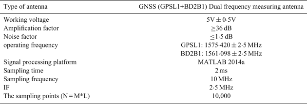
In this experiment, the 2ms satellite signal was sampled by the IF signal sampler shown in Figure 20. The setup for the signal sampling experiment is shown as Figure 21. The parameters of the experimental equipment are shown in Table 3. The signal was then processed on MATLAB.

Figure 20. GNSS IF signal sampler SIS600B1 + L1.

Figure 21. Experimental setup for live data acquisition and storage.
Table 3. Parameters of experimental equipment.

Figures 22–24 show the BeiDou PRN-3 satellite acquisition results of the traditional PFA, L = 64 modified PFA and L = 32 modified PFA algorithms, respectively.

Figure 22. Acquisition results of BeiDou PRN-3 satellite by the traditional PFA algorithm.

Figure 23. Acquisition results of BeiDou PRN-3 satellite by the L = 64 modified PFA algorithm.

Figure 24. Acquisition results of BeiDou PRN-3 satellite by the L = 32 modified PFA algorithm.
From Figures 22, 23 and 24, it can be seen that the acquired PRN code delay is 909 chips and the Doppler shift is 0 Hz. The acquired Doppler shift and the phase of PRN code are the same with the above three algorithms. In order to verify the SNR decreases with the increase of M, different M values were taken to measure the SNR of the acquired PRN-3 satellite. Experiments showed that the SNR of the PRN-3 satellite acquired by the traditional PFA algorithm was 20·47 dB. When the number of sampling points N was 10,000, the SNR of the PRN-3 satellite acquired by the modified PFA algorithm was lower than that of the traditional PFA algorithm. The effect of FFT points L on the SNR is shown in Figure 25.

Figure 25. Effect of FFT points L on SNR.
It can be seen from Figure 25 that the theoretical value and the experimental value were close to each other although they did not completely match due to the introduction of the system measurement error. When both the number of sampling points N and the Doppler shifts were small, the modified PFA algorithm had almost no effect on the SNR compared to the traditional PFA algorithm.
In order to verify that the modified PFA algorithm could indeed shorten the acquisition time, the same segment of acquisition code ran repeatedly in MATLAB 5,000 times, and the acquisition time was measured. According to experimental measurement, the average time required for the traditional PFA algorithm to acquire the 2ms PRN-3 satellite signals was 1·69 seconds. The time reduction of the modified PFA over the traditional PFA algorithm is shown in Figure 26.

Figure 26. Effect of FFT points L on the time required for PRN-3 acquisition.
It can be seen from Figure 26 that the acquisition time of the modified PFA algorithm was reduced by more than 80% compared to that of the traditional PFA algorithm when the number of sampling points N and the Doppler shifts were small.
8. CONCLUSION
A new acquisition algorithm for the complex signal of BeiDou B1I is proposed in this paper. Compared with the traditional PFA algorithm, the proposed PFA algorithm based on coherent downsampling includes two extra modules: a complex downconversion module and a coherent downsampling module. The time needed to acquire the satellite was reduced by at least 80% with the modified PFA algorithm and the SNR loss was less than 0·5 dB when the number of sampling points N and the Doppler shifts were small.
FINANCIAL SUPPORT
This work was supported by the Fundamental Research Funds for the Central Universities (NO. NS2019022).