


1. Introduction
In ‘quiet’ disturbance environments, which are typical of flight conditions, the initial stages of laminar–turbulent transition are dominated by the evolution of instability modes (primary instabilities, possibly followed by secondary instabilities), which grow exponentially due to linear processes. The nature of these instabilities depends greatly on the state of the laminar boundary layer. In boundary layers developing over swept wings with large sweep angles, the transition process is dominated by the cross-flow instability. The Tollmien–Schlichting (TS) waves drive the boundary-layer instability in the case of small sweep angles, while Taylor–Görtler vortices are the dominant primary instability for boundary layers developing over concave walls. Since the first pioneering experiments of Reynolds (Reference Reynolds1883), the complexity and great variety of possible mechanisms involved in the laminar–turbulent transition have inspired a great deal of work on this subject, despite which transition prediction still remains a formidable task. The main problem associated with current transition prediction methodologies is that they are largely based on the concept of disturbance amplification, rather than on the disturbance amplitude, and hence completely disregard the receptivity process, the importance of which was highlighted by numerous experiments (see Reshotko Reference Reshotko1976; Kachanov Reference Kachanov1994; Saric, Reed & Kerschen Reference Saric, Reed and Kerschen2002, and references therein). Receptivity theory studies the process of interaction between the boundary layer and ‘external perturbations’, such as acoustic waves, free-stream turbulence and body surface vibrations. The objective of the receptivity analysis is, first, to identify how the external perturbations can be converted into instability modes of the boundary layer, the TS waves, cross-flow vortices or Taylor–Görtler vortices, and, second, to determine the initial amplitude of these modes.
The progress achieved in this field has been, to a large degree, thanks to the studies based on the asymptotic analysis of the Navier–Stokes equations at large values of the Reynolds number. When dealing with the process of generation of TS waves in boundary layers, this approach relies on the triple-deck theory, which is known to describe the TS waves in subsonic flows near the lower branch of the neutral stability curve (see Lin Reference Lin1946; Smith Reference Smith1979a ,Reference Smith b ). The first paper where the triple-deck theory was used to study the receptivity of the boundary layer was published by Terent’ev (Reference Terent’ev1981). He considered an incompressible flow past a flat plate with the basic steady flow given by the Blasius solution. He assumed that a short section of the plate surface performs periodic vibrations in the direction perpendicular to the wall. This formulation represents a simplified mathematical model of the classical experiments performed by Schubauer & Skramstad (Reference Schubauer and Skramstad1948) where the TS waves were generated by a vibrating ribbon installed a small distance above the plate surface. Terent’ev’s theory shows that, in the vicinity of the vibrating part of the wall, the perturbation field is rather complex. However, further downstream, only one perturbation mode survives, the TS wave. The amplitude of this wave depends on the shape of the vibrating part of the wall.
It is known from numerous observations that the boundary layers are susceptible to acoustic noise. Asymptotic theory of the generation of TS waves by acoustic noise was developed by Ruban (Reference Ruban1984) and Goldstein (Reference Goldstein1985). In these studies the importance of the notion of ‘double resonance’ was highlighted as a fundamental principle of the receptivity theory. In fluid flows, effective transformation of external disturbances into instability modes of the boundary layer is only possible if, in addition to the frequency, the wavenumber of the external perturbations is in tune with the natural internal oscillations of the boundary layer. These conditions could be easily satisfied in the problem considered by Terent’ev (Reference Terent’ev1981), where the frequency and the length of the vibrating part of the wall can be chosen independently of one another. When an acoustic wave impinges upon the boundary layer, the pressure perturbations in the acoustic wave penetrate into the boundary layer, leading to the creation of a near-wall Stokes layer inside the boundary layer. If the acoustic field has a wide enough spectrum, then the receptivity process will ‘extract’ from it a harmonic whose frequency is in tune with the frequency of the corresponding TS wave. Of course, under this condition the wavelength of the ‘chosen’ acoustic wave appears to be much longer than that of the TS wave, meaning that the second resonance condition, the tuning of the wavenumbers, is not satisfied. However, in practical applications, such as in the flow past an aircraft wing, the body surface in never absolutely smooth. Hence, in addition to unsteady perturbations in the Stokes layer, one has to consider steady perturbations produced by the wall roughnesses, which normally have a short length scale. Ruban (Reference Ruban1984) and Goldstein (Reference Goldstein1985) demonstrated that the interaction between the two perturbation modes leads to the formation of TS waves behind the roughness. Along with acoustic waves, free-stream turbulence is also known to have a significant influence on the laminar–turbulent transition in the boundary layer. The asymptotic theory of the receptivity of the boundary layer to the free-stream turbulence was developed by Duck, Ruban & Zhikharev (Reference Duck, Ruban and Zhikharev1996). They found that, unlike the acoustic waves, the vorticity waves do not carry pressure perturbations, and therefore are unable to penetrate into the boundary layer. However, the steady flow perturbations produced by a wall roughness are not confined to the boundary layer but extend to the flow outside the boundary layer, where they come into interaction with the vorticity wave. Duck et al. (Reference Duck, Ruban and Zhikharev1996) showed that this interaction results in a TS wave forming downstream of the roughness.
Recently, the generation of TS waves in the boundary layer due to elastic vibrations of the wing surface was analysed by Ruban, Bernots & Pryce (Reference Ruban, Bernots and Pryce2013). Their results show that the wing surface vibrations can cause pressure perturbations in the flow outside the boundary layer, which, in turn, induce a Stokes layer near the wing surface. Two physical mechanisms were found to be able to induce an oscillatory motion of the Stokes layer. The first one is the classical mechanism where the pressure gradient, being a periodic function of time, forces the fluid to oscillate in the direction along the wing surface. This process is similar to the one described by Ruban (Reference Ruban1984) and Goldstein (Reference Goldstein1985) in their study of the boundary-layer receptivity to acoustic waves. In the second mechanism, the pressure itself, not the pressure gradient, makes up the Stokes layer. In both cases, TS waves are generated when the Stokes layer encounters a wall roughness. These and other examples (Denier, Hall & Seddougui Reference Denier, Hall and Seddougui1991; Wu Reference Wu2001; Kerimbekov & Ruban Reference Kerimbekov and Ruban2005; Wu, Zhao & Luo Reference Wu, Zhao and Luo2011) show that the asymptotic approach has proven to be invaluable in uncovering the possible mechanism of boundary-layer receptivity. However, the accuracy with which the asymptotic theory predicts the initial amplitude of the instability modes forming in the boundary layer has been under question.
Boundary-layer receptivity problems have also been extensively analysed experimentally (see e.g. Kachanov, Kozlov & Levchenko Reference Kachanov, Kozlov and Levchenko1979; Saric & White Reference Saric and White1998; Dietz Reference Dietz1999; Borodulin et al. Reference Borodulin, Ivanov, Kachanov and Roschektaev2013) and numerically (see e.g. Fucciarelli, Reed & Lyttle Reference Fucciarelli, Reed and Lyttle2000; Wanderley & Corke Reference Wanderley and Corke2001; Jones, Sandberg & Sandham Reference Jones, Sandberg and Sandham2010; Tempelmann et al. Reference Tempelmann, Schrader, Hanifi, Brandt and Henningson2012). The main challenge of the experimental investigations is the measurement of the receptivity coefficients, since the initial amplitudes of the boundary-layer instabilities may be orders of magnitude smaller than the amplitude of the surrounding disturbance environment. On the other hand, the main difficulty associated with numerical simulations is to accurately represent the free-stream disturbance environment, whereby care needs to be taken to correctly formulate the boundary conditions needed to capture the effects of the different types of perturbations (acoustic waves, entropy waves and vorticity waves) on the boundary-layer receptivity. Despite the numerous efforts, comparisons between the predictions of the asymptotic theory of receptivity and the numerical and experimental results are very limited. Comparisons with experiments can be found, for example, in Goldstein & Hultgren (Reference Goldstein and Hultgren1987), Kozlov & Ryzhov (Reference Kozlov and Ryzhov1990) and Wu (Reference Wu2001), while detailed comparisons with the predictions of the finite-Reynolds-number Orr–Sommerfeld theory (Zhigulev & Fedorov Reference Zhigulev and Fedorov1987; Choudhari & Street Reference Choudhari and Street1992; Crouch Reference Crouch1992) are reported in Choudhari & Street (Reference Choudhari and Street1992). However, the range of parameters over which the asymptotic theory has been compared with high-fidelity Navier–Stokes numerical simulations and/or experiments is very limited, hence a detailed evaluation of the capabilities of the theory is currently missing. In this paper we address this issue by comparing the asymptotic theory with numerical simulations of the compressible Navier–Stokes equations, focusing on two important receptivity problems: the TS wave generation by a vibrating ribbon placed on the wall of a flat plate and that due to the interaction between a small isolated roughness element and an acoustic wave travelling in the flow direction. The investigation is carried out through a parametric study on the effects of roughness element/vibrator longitudinal dimension, Reynolds number, Mach number and TS wave frequency. In this work, special care has been taken in the formulation of the boundary conditions used to obtain the relevant disturbance fields (particularly for the numerical analysis of the receptivity due to sound), which are critical for the accurate determination of the receptivity coefficients. The numerical techniques used to obtain the disturbance fields are described in § 4.2.
The paper is organised as follows. In § 2 the receptivity problems are introduced along with the theoretical preliminaries of the triple-deck study. The main steps of the triple-deck analysis are given in § 3. All the details of the numerical study are given in § 4. In § 5 we provide comparisons between the numerical and the theoretical results, along with a discussion of the main findings. The paper ends in § 6, where the main conclusions of the study are drawn.
2. Problem formulation and triple-deck scalings
Consider the two-dimensional laminar boundary layer that forms on the surface of a flat plate in a subsonic free stream. We shall analyse the two receptivity problems arising from the interaction between an acoustic wave and an isolated two-dimensional roughness element and from the time-periodic vibrations of a ribbon placed on the flat plate wall, as schematically depicted in figure 1 (note that, for brevity, in the remainder of this paper the roughness element and the vibrating ribbon will be referred to as ‘the wall disturbance’ whenever the subject of the discussion applies to both). The mechanisms responsible for the generation of TS waves in the above two scenarios are fully described by the compressible Navier–Stokes equations, which, for a two-dimensional flow, may be written as
 $$\begin{eqnarray}\displaystyle & \displaystyle \frac{\partial {\it\rho}}{\partial t}+\frac{\partial {\it\rho}u}{\partial x}+\frac{\partial {\it\rho}v}{\partial y}=0, & \displaystyle\end{eqnarray}$$
 $$\begin{eqnarray}\displaystyle & \displaystyle {\it\rho}\frac{\text{D}u}{\text{D}t}=-\frac{\partial p}{\partial x}+\frac{1}{\mathit{Re}}\frac{\partial }{\partial y}\left({\it\mu}\frac{\partial u}{\partial y}\right)+\cdots \,, & \displaystyle\end{eqnarray}$$
 $$\begin{eqnarray}\displaystyle & \displaystyle {\it\rho}\frac{\text{D}v}{\text{D}t}=-\frac{\partial p}{\partial y}+\frac{1}{\mathit{Re}}\frac{\partial }{\partial y}\left({\it\mu}\frac{\partial v}{\partial y}\right)+\cdots \,, & \displaystyle\end{eqnarray}$$
 $$\begin{eqnarray}\displaystyle & \displaystyle {\it\rho}\frac{\text{D}h}{\text{D}t}=\frac{\text{D}p}{\text{D}t}+\frac{1}{\mathit{Re}\,\mathit{Pr}}\frac{\partial }{\partial y}\left({\it\mu}\frac{\partial h}{\partial y}\right)+\frac{{\it\mu}}{\mathit{Re}}\left(\frac{\partial u}{\partial y}\right)^{2}+\cdots \,, & \displaystyle\end{eqnarray}$$
 $$\begin{eqnarray}\displaystyle & \displaystyle p=\frac{{\it\gamma}-1}{{\it\gamma}}{\it\rho}h=\frac{{\it\rho}T}{{\it\gamma}\mathit{Ma}^{2}}. & \displaystyle\end{eqnarray}$$
 $$\begin{eqnarray}\left.\begin{array}{@{}c@{}}\displaystyle x=\frac{x^{\ast }-x_{0}^{\ast }}{L^{\ast }},\quad y=\frac{y^{\ast }}{L^{\ast }},\quad u=\frac{u^{\ast }}{U_{\infty }^{\ast }},\quad v=\frac{v^{\ast }}{U_{\infty }^{\ast }},\quad {\it\rho}=\frac{{\it\rho}^{\ast }}{{\it\rho}_{\infty }^{\ast }},\\ \displaystyle p=\frac{p^{\ast }}{{\it\rho}_{\infty }^{\ast }U_{\infty }^{\ast 2}},\quad {\it\mu}=\frac{{\it\mu}^{\ast }}{{\it\mu}_{\infty }^{\ast }},\quad t=\frac{t^{\ast }U_{\infty }^{\ast }}{L^{\ast }},\quad h=\frac{h^{\ast }}{U_{\infty }^{\ast 2}}.\end{array}\right\}\end{eqnarray}$$
Here the reference length
 $L^{\ast }$
is the distance between the leading edge of the flat plate and the centre of the wall disturbance, which is positioned at
$L^{\ast }$
is the distance between the leading edge of the flat plate and the centre of the wall disturbance, which is positioned at
 $x^{\ast }=x_{0}^{\ast }$
. The
$x^{\ast }=x_{0}^{\ast }$
. The
 $x^{\ast }$
coordinate measures the distance along the flat plate wall starting from its leading edge, and the
$x^{\ast }$
coordinate measures the distance along the flat plate wall starting from its leading edge, and the
 $y^{\ast }$
coordinate indicates the distance to the wall of the plate. The streamwise and wall-normal velocities are denoted respectively as
$y^{\ast }$
coordinate indicates the distance to the wall of the plate. The streamwise and wall-normal velocities are denoted respectively as
 $u^{\ast }$
and
$u^{\ast }$
and
 $v^{\ast }$
, the fluid density as
$v^{\ast }$
, the fluid density as
 ${\it\rho}^{\ast }$
, the pressure as
${\it\rho}^{\ast }$
, the pressure as
 $p^{\ast }$
, the dynamic viscosity as
$p^{\ast }$
, the dynamic viscosity as
 ${\it\mu}^{\ast }$
and the enthalpy as
${\it\mu}^{\ast }$
and the enthalpy as
 $h^{\ast }$
. Asterisks indicate dimensional quantities. The dimensionless parameters for this problem are the Reynolds number
$h^{\ast }$
. Asterisks indicate dimensional quantities. The dimensionless parameters for this problem are the Reynolds number
 $\mathit{Re}$
, the Mach number
$\mathit{Re}$
, the Mach number
 $\mathit{Ma}$
and the Prandtl number
$\mathit{Ma}$
and the Prandtl number
 $\mathit{Pr}$
, which we consider to be constant and equal to
$\mathit{Pr}$
, which we consider to be constant and equal to
 $\mathit{Pr}=0.72$
.
$\mathit{Pr}=0.72$
.

Figure 1. Schematic representation of the receptivity problem.
In the absence of any external perturbations, the laminar basic flow over a smooth flat plate is governed by the classical compressible boundary-layer equations, which, using Illingworth’s transformation (see e.g. White Reference White2005), may be written as
 $$\begin{eqnarray}\displaystyle & \displaystyle (C\mathscr{F}^{\prime \prime })^{\prime }+\mathscr{F}\mathscr{F}^{\prime \prime }=0, & \displaystyle\end{eqnarray}$$
 $$\begin{eqnarray}\displaystyle & \displaystyle (C\mathscr{G}^{\prime })^{\prime }+\mathit{Pr}\,\mathscr{F}\mathscr{G}^{\prime }=-({\it\gamma}-1)C\,\mathit{Pr}\,\mathit{Ma}^{2}\mathscr{F}^{\prime \prime 2}, & \displaystyle\end{eqnarray}$$
 $\mathscr{F}^{\prime }({\it\eta})=U_{B}$
is the basic flow streamwise velocity,
$\mathscr{F}^{\prime }({\it\eta})=U_{B}$
is the basic flow streamwise velocity,
 $\mathscr{G}({\it\eta})=h_{B}$
is the basic flow enthalpy and
$\mathscr{G}({\it\eta})=h_{B}$
is the basic flow enthalpy and
 $C(\mathscr{G})={\it\mu}_{B}{\it\rho}_{B}$
is the Chapman–Rubesin parameter. Equations (2.3) are obtained after introducing the similarity coordinates
$C(\mathscr{G})={\it\mu}_{B}{\it\rho}_{B}$
is the Chapman–Rubesin parameter. Equations (2.3) are obtained after introducing the similarity coordinates  $$\begin{eqnarray}{\it\xi}={\it\mu}_{\infty }^{\ast }{\it\rho}_{\infty }^{\ast }U_{\infty }^{\ast }L^{\ast }(1+x)\quad \text{and}\quad {\it\eta}=\frac{(1+x)^{-1/2}}{\sqrt{2}}\int _{0}^{Y}{\it\rho}\,\text{d}Y,\end{eqnarray}$$
where
 $Y=\mathit{Re}^{1/2}y$
is the usual boundary-layer wall-normal coordinate. In this work we assume that the flat plate wall is adiabatic, so that the wall temperature is constant and equal to
$Y=\mathit{Re}^{1/2}y$
is the usual boundary-layer wall-normal coordinate. In this work we assume that the flat plate wall is adiabatic, so that the wall temperature is constant and equal to
 $$\begin{eqnarray}T_{w}=1+\mathit{Pr}^{1/2}\frac{{\it\gamma}-1}{2}\mathit{Ma}^{2}.\end{eqnarray}$$
Under this condition, (2.3) admit smooth self-similar solutions, which may be expanded in Taylor series around
 $x=0$
(i.e. around the centre of the wall disturbance) as
$x=0$
(i.e. around the centre of the wall disturbance) as
 $$\begin{eqnarray}\left.\begin{array}{@{}rcl@{}}U_{B}(x,Y)\ & =\ & U_{B0}(Y)+O(x),\\ {\it\rho}_{B}(x,Y)\ & =\ & {\it\rho}_{B0}(Y)+O(x),\\ h_{B}(x,Y)\ & =\ & h_{B0}(Y)+O(x),\\ {\it\mu}_{B}(x,Y)\ & =\ & {\it\mu}_{B0}(Y)+O(x)\end{array}\right\}\quad \text{as}~x\rightarrow 0~\text{and}~Y=O(1).\end{eqnarray}$$
In addition, the near-wall behaviour of the boundary-layer flow near
 $x=0$
can also be recovered by noting that the leading-order terms in (2.6) may in turn be Taylor-expanded near the wall. Hence one can write
$x=0$
can also be recovered by noting that the leading-order terms in (2.6) may in turn be Taylor-expanded near the wall. Hence one can write
 $$\begin{eqnarray}\left.\begin{array}{@{}rcl@{}}U_{B}\ & =\ & {\it\lambda}Y+\cdots \,,\\ {\it\rho}_{B}\ & =\ & {\it\rho}_{w}+\cdots \,,\\ h_{B}\ & =\ & h_{w}+\cdots \,,\\ {\it\mu}_{B}\ & =\ & {\it\mu}_{w}+\cdots \end{array}\right\}\quad \text{as}~x\rightarrow 0~\text{and}~Y\rightarrow 0,\end{eqnarray}$$
where
 $$\begin{eqnarray}{\it\lambda}=\left.\frac{\,\text{d}U_{B0}}{\,\text{d}Y}\right|_{w}=\frac{\mathscr{F}^{\prime \prime }(0)}{\sqrt{2}T_{w}}\end{eqnarray}$$
and
 $\mathscr{F}^{\prime \prime }(0)$
is obtained by solving (2.3) numerically. The values of
$\mathscr{F}^{\prime \prime }(0)$
is obtained by solving (2.3) numerically. The values of
 $\mathscr{F}^{\prime \prime }(0)$
associated with the numerical simulations carried out in this work are given in § 4.2 (table 1).
$\mathscr{F}^{\prime \prime }(0)$
associated with the numerical simulations carried out in this work are given in § 4.2 (table 1).
As anticipated in the introduction, the asymptotic theory of receptivity is based on the triple-deck theory, which describes the TS waves in subsonic flows near the lower branch of the neutral stability curve (see Lin Reference Lin1946; Smith Reference Smith1979a
,Reference Smith
b
). Therefore, following the triple-deck formalism, the flow near the wall disturbance is divided into three regions in the wall-normal direction, as depicted in figure 2. Strictly speaking, the wall disturbance should be contained within the lower deck (region 1) in order for the triple-deck theory to be valid. In addition, the frequency of the vibrating ribbon and the free-stream acoustic wave has to match the lower-branch TS wave frequency, which is an
 $O(\mathit{Re}^{1/4})$
quantity (Lin Reference Lin1946). Therefore, the frequency of the imposed oscillations, the streamwise length of the wall disturbance and the wall-normal size (
$O(\mathit{Re}^{1/4})$
quantity (Lin Reference Lin1946). Therefore, the frequency of the imposed oscillations, the streamwise length of the wall disturbance and the wall-normal size (
 $h$
) of the wall disturbance (taken here as the amplitude of the vibrations of the ribbon or the height of the roughness element) are taken to be of
$h$
) of the wall disturbance (taken here as the amplitude of the vibrations of the ribbon or the height of the roughness element) are taken to be of
 $O(\mathit{Re}^{1/4})$
,
$O(\mathit{Re}^{1/4})$
,
 $O(\mathit{Re}^{-3/8})$
and
$O(\mathit{Re}^{-3/8})$
and
 $O(\mathit{Re}^{-5/8})$
, respectively.
$O(\mathit{Re}^{-5/8})$
, respectively.

Figure 2. Triple-deck formalism.
Based on the above considerations, the shape of the roughness element and the vibrating ribbon may be expressed respectively as
 $$\begin{eqnarray}y_{r}=hF\left(\frac{x}{\mathit{Re}^{-3/8}}\right)\quad \text{and}\quad y_{r}=hF\left(\frac{x}{\mathit{Re}^{-3/8}}\right)G\left(\frac{t}{\mathit{Re}^{-1/4}}\right),\end{eqnarray}$$
where
 $h={\it\epsilon}\mathit{Re}^{-5/8}$
with
$h={\it\epsilon}\mathit{Re}^{-5/8}$
with
 ${\it\epsilon}=O(1)$
. In order to obtain an analytical description of the receptivity of TS waves by the interaction between an acoustic wave and a roughness element, the disturbances induced inside the boundary layer by the acoustic wave also need to be analysed using asymptotic analysis. It can be shown that the acoustic wave leads to the generation of a thin oscillating layer near the wall, the Stokes layer, the thickness of which is of the same order of magnitude as that of the lower deck, as schematically depicted in figure 2.
${\it\epsilon}=O(1)$
. In order to obtain an analytical description of the receptivity of TS waves by the interaction between an acoustic wave and a roughness element, the disturbances induced inside the boundary layer by the acoustic wave also need to be analysed using asymptotic analysis. It can be shown that the acoustic wave leads to the generation of a thin oscillating layer near the wall, the Stokes layer, the thickness of which is of the same order of magnitude as that of the lower deck, as schematically depicted in figure 2.
The asymptotic theory of the generation of TS waves by sound is due to Ruban (Reference Ruban1984) and Goldstein (Reference Goldstein1985), while the receptivity problem of a vibrating ribbon was first solved in the context of the triple-deck theory by Terent’ev (Reference Terent’ev1981). The aim of this paper is to provide a detailed assessment of the applicability of the above theories by comparing their predictions with high-fidelity Navier–Stokes simulation results. Therefore, only the relevant portions of the theoretical analyses are provided in the following for completeness.
3. Triple-deck theory
The flow in the vicinity of a wall disturbance given by one of equations (2.9) may be described by the triple-deck theory. In the lower deck, after introducing the usual scaled coordinates
 $$\begin{eqnarray}\bar{t}=\mathit{Re}^{1/4}\frac{{\it\mu}_{w}^{1/2}}{{\it\lambda}^{-3/2}{\it\beta}^{-1/2}}t,\quad \bar{x}=\mathit{Re}^{3/8}\frac{{\it\mu}_{w}^{1/4}{\it\rho}_{w}^{1/2}}{{\it\lambda}^{-5/4}{\it\beta}^{-3/4}}x\quad \text{and}\quad \bar{y}=\mathit{Re}^{5/8}\frac{{\it\mu}_{w}^{-1/4}{\it\rho}_{w}^{1/2}}{{\it\lambda}^{-3/4}{\it\beta}^{-1/4}}y\end{eqnarray}$$
and substituting the following asymptotic expansions
 $$\begin{eqnarray}\left.\begin{array}{@{}c@{}}\displaystyle u=\mathit{Re}^{-1/8}\frac{{\it\mu}_{w}^{1/4}{\it\rho}_{w}^{-1/2}}{{\it\lambda}^{-1/4}{\it\beta}^{1/4}}\bar{U}+\cdots \,,\quad \displaystyle v=\mathit{Re}^{-3/8}\frac{{\it\mu}_{w}^{3/4}{\it\rho}_{w}^{-1/2}}{{\it\lambda}^{-3/4}{\it\beta}^{-1/4}}\bar{V}+\cdots \,,\\ \displaystyle p=p_{\infty }+\mathit{Re}^{-1/4}\frac{{\it\mu}_{w}^{1/2}}{{\it\lambda}^{-1/2}{\it\beta}^{1/2}}\bar{P}+\cdots \,,\end{array}\right\}\end{eqnarray}$$
into the Navier–Stokes equations (2.1), the governing equations can be written as
 $$\begin{eqnarray}\displaystyle & \displaystyle \frac{\partial \bar{U}}{\partial \bar{x}}+\frac{\partial \bar{V}}{\partial \bar{y}}=0, & \displaystyle\end{eqnarray}$$
 $$\begin{eqnarray}\displaystyle & \displaystyle \frac{\partial \bar{U}}{\partial \bar{t}}+\bar{U}\frac{\partial \bar{U}}{\partial \bar{x}}+\bar{V}\frac{\partial \bar{U}}{\partial \bar{y}}=-\frac{\partial \bar{P}}{\partial \bar{x}}+\frac{\partial ^{2}\bar{U}}{\partial \bar{y}^{2}}, & \displaystyle\end{eqnarray}$$
 $$\begin{eqnarray}\displaystyle & \displaystyle \bar{U}=\bar{U}_{w},\quad \bar{V}=\bar{V}_{w}\quad \text{at}~\bar{y}=\bar{y}_{r}, & \displaystyle\end{eqnarray}$$
 $$\begin{eqnarray}\displaystyle & \displaystyle \bar{U}=\bar{y}+\cdots \quad \text{as}~\bar{x}\rightarrow -\infty , & \displaystyle\end{eqnarray}$$
 $$\begin{eqnarray}\displaystyle & \displaystyle \bar{U}=\bar{y}+\bar{A}(\bar{t},\bar{x})+\cdots \quad \text{as}~\bar{y}\rightarrow \infty . & \displaystyle\end{eqnarray}$$
 ${\it\beta}=\sqrt{1-\mathit{ Ma }^{2}}$
,
${\it\beta}=\sqrt{1-\mathit{ Ma }^{2}}$
,
 $\bar{A}$
is the usual unknown displacement function and
$\bar{A}$
is the usual unknown displacement function and
 $\bar{U}_{w}$
and
$\bar{U}_{w}$
and
 $\bar{V}_{w}$
represent the motion of the flat plate wall (
$\bar{V}_{w}$
represent the motion of the flat plate wall (
 $\bar{U}_{w}=\bar{V}_{w}=0$
in the case of a steady roughness element). It is important to note that, since the local Mach number is small near the wall, we have assumed that the flow is incompressible and hence have neglected density, viscosity and enthalpy disturbances. Given the scaling introduced for the time
$\bar{U}_{w}=\bar{V}_{w}=0$
in the case of a steady roughness element). It is important to note that, since the local Mach number is small near the wall, we have assumed that the flow is incompressible and hence have neglected density, viscosity and enthalpy disturbances. Given the scaling introduced for the time
 $t$
and the
$t$
and the
 $x$
coordinate, it is convenient to explicitly introduce the scaled frequency
$x$
coordinate, it is convenient to explicitly introduce the scaled frequency
 $\bar{{\it\omega}}=\mathit{Re}^{-1/4}{\it\mu}_{w}^{-1/2}{\it\lambda}^{-3/2}{\it\beta}^{-1/2}{\it\omega}$
and the scaled streamwise wavenumber
$\bar{{\it\omega}}=\mathit{Re}^{-1/4}{\it\mu}_{w}^{-1/2}{\it\lambda}^{-3/2}{\it\beta}^{-1/2}{\it\omega}$
and the scaled streamwise wavenumber
 $\bar{{\it\alpha}}=\mathit{Re}^{-3/8}{\it\mu}_{w}^{-1/4}{\it\rho}_{w}^{-1/2}{\it\lambda}^{-5/4}{\it\beta}^{-3/4}{\it\alpha}$
for future reference.
$\bar{{\it\alpha}}=\mathit{Re}^{-3/8}{\it\mu}_{w}^{-1/4}{\it\rho}_{w}^{-1/2}{\it\lambda}^{-5/4}{\it\beta}^{-3/4}{\it\alpha}$
for future reference.
3.1. Receptivity of TS waves by sound
In the lower-deck coordinates (3.1), the shape of the roughness element may be written as
 $\bar{y}_{r}={\it\epsilon}\bar{F}(\bar{x})$
, where we have used
$\bar{y}_{r}={\it\epsilon}\bar{F}(\bar{x})$
, where we have used
 $F={\it\mu}_{w}^{1/4}{\it\rho}_{w}^{-1/2}{\it\lambda}^{-3/4}{\it\beta}^{-1/4}\bar{F}$
and, since here we are interested in the linear case, we put
$F={\it\mu}_{w}^{1/4}{\it\rho}_{w}^{-1/2}{\it\lambda}^{-3/4}{\it\beta}^{-1/4}\bar{F}$
and, since here we are interested in the linear case, we put
 ${\it\epsilon}\ll 1$
. Let us now assume that there is a plane acoustic wave travelling in the free stream in the flow direction. The acoustic wave amplitude is chosen so that the streamwise pressure gradient induced by the wave is of the same order of magnitude as that induced by the roughness element. It turns out that this condition is fulfilled if the acoustic wave amplitude is an order
${\it\epsilon}\ll 1$
. Let us now assume that there is a plane acoustic wave travelling in the free stream in the flow direction. The acoustic wave amplitude is chosen so that the streamwise pressure gradient induced by the wave is of the same order of magnitude as that induced by the roughness element. It turns out that this condition is fulfilled if the acoustic wave amplitude is an order
 $O(\mathit{Re}^{-1/8})$
quantity; here we put
$O(\mathit{Re}^{-1/8})$
quantity; here we put
 $a={\it\delta}\mathit{Re}^{-1/8}$
, with
$a={\it\delta}\mathit{Re}^{-1/8}$
, with
 ${\it\delta}\ll 1$
. Such a wave induces a Stokes layer near the wall; the interaction between the Stokes layer disturbances and the roughness element gives rise to a TS wave.
${\it\delta}\ll 1$
. Such a wave induces a Stokes layer near the wall; the interaction between the Stokes layer disturbances and the roughness element gives rise to a TS wave.
The disturbances introduced into the boundary layer in the vicinity of the roughness element are due to: the roughness element itself, denoted as say
 $u_{1}$
; the oscillations of the Stokes layer, say
$u_{1}$
; the oscillations of the Stokes layer, say
 $u_{s}$
; and the interactions between the previous two, say
$u_{s}$
; and the interactions between the previous two, say
 $u_{2}$
. Therefore, after applying Prandtl’s transformations
$u_{2}$
. Therefore, after applying Prandtl’s transformations
 $$\begin{eqnarray}\left.\begin{array}{@{}c@{}}\bar{t}=\tilde{t},\quad \bar{x}=\tilde{x},\quad \bar{y}={\tilde{y}}+{\it\epsilon}\tilde{F},\\ \bar{U}=\tilde{U} ,\quad \bar{V}=\tilde{V}+{\it\epsilon}\tilde{U} \tilde{F}^{\prime },\quad \bar{P}=\tilde{P},\\ \bar{F}=\tilde{F},\end{array}\right\}\end{eqnarray}$$
which are used to simplify the wall boundary conditions, we look for lower-deck solutions in the following form:
 $$\begin{eqnarray}\displaystyle & \displaystyle \tilde{U} ={\tilde{y}}+{\it\delta}u_{s}(\tilde{t},x_{s},{\tilde{y}})+{\it\epsilon}u_{1}(\tilde{x},{\tilde{y}})+{\it\epsilon}{\it\delta}u_{2}(\tilde{t},\tilde{x},{\tilde{y}})+\cdots \,, & \displaystyle\end{eqnarray}$$
 $$\begin{eqnarray}\displaystyle & \displaystyle \tilde{V}=\mathit{Re}^{-1/8}{\it\delta}v_{s}(\tilde{t},x_{s},{\tilde{y}})+{\it\epsilon}v_{1}(\tilde{x},{\tilde{y}})+{\it\epsilon}{\it\delta}v_{2}(\tilde{t},\tilde{x},{\tilde{y}})+\cdots \,, & \displaystyle\end{eqnarray}$$
 $$\begin{eqnarray}\displaystyle & \displaystyle \tilde{P}=\mathit{Re}^{1/8}{\it\delta}p_{s}(\tilde{t},x_{s})+{\it\epsilon}p_{1}(\tilde{x})+{\it\epsilon}{\it\delta}p_{2}(\tilde{t},\tilde{x})+\cdots \,. & \displaystyle\end{eqnarray}$$
 $x_{s}=\mathit{Re}^{1/4}x$
and the Stokes layer terms (subscript
$x_{s}=\mathit{Re}^{1/4}x$
and the Stokes layer terms (subscript
 $s$
) are introduced to ensure that the solution matches the Stokes layer solution for
$s$
) are introduced to ensure that the solution matches the Stokes layer solution for
 $\tilde{x}\rightarrow -\infty$
. By substituting the above into (3.3) and (3.4), we obtain a steady problem describing the roughness-induced disturbances
$\tilde{x}\rightarrow -\infty$
. By substituting the above into (3.3) and (3.4), we obtain a steady problem describing the roughness-induced disturbances
 $u_{1}$
(by collecting terms with
$u_{1}$
(by collecting terms with
 ${\it\epsilon}$
) and an unsteady problem describing the disturbances arising from the interaction between the Stokes layer and the roughness element (by collecting terms with
${\it\epsilon}$
) and an unsteady problem describing the disturbances arising from the interaction between the Stokes layer and the roughness element (by collecting terms with
 ${\it\epsilon}{\it\delta}$
).
${\it\epsilon}{\it\delta}$
).
In Fourier space,
 $\hat{u} _{1}=(2{\rm\pi})^{-1/2}\int _{-\infty }^{\infty }u_{1}\text{e}^{-\text{i}\bar{{\it\alpha}}\tilde{x}}\,\text{d}\tilde{x}$
, the steady problem has the solution
$\hat{u} _{1}=(2{\rm\pi})^{-1/2}\int _{-\infty }^{\infty }u_{1}\text{e}^{-\text{i}\bar{{\it\alpha}}\tilde{x}}\,\text{d}\tilde{x}$
, the steady problem has the solution
 $\hat{u} _{1}={\it\Gamma}({\it\zeta};\bar{{\it\alpha}})\hat{F}(\bar{{\it\alpha}})$
and
$\hat{u} _{1}={\it\Gamma}({\it\zeta};\bar{{\it\alpha}})\hat{F}(\bar{{\it\alpha}})$
and
 $\hat{v}_{1}={\it\Theta}({\it\zeta};\bar{{\it\alpha}})\hat{F}(\bar{{\it\alpha}})$
, where
$\hat{v}_{1}={\it\Theta}({\it\zeta};\bar{{\it\alpha}})\hat{F}(\bar{{\it\alpha}})$
, where
 ${\it\zeta}=(\text{i}\bar{{\it\alpha}})^{1/3}{\tilde{y}}$
and
${\it\zeta}=(\text{i}\bar{{\it\alpha}})^{1/3}{\tilde{y}}$
and
 $$\begin{eqnarray}\displaystyle & \displaystyle {\it\Gamma}({\it\zeta};\bar{{\it\alpha}})=-\frac{3(\text{i}\bar{{\it\alpha}})^{1/3}|\bar{{\it\alpha}}|}{3\text{Ai}^{\prime }(0)-|\bar{{\it\alpha}}|(\text{i}\bar{{\it\alpha}})^{1/3}}\int _{0}^{{\it\zeta}}\text{Ai}(s)\,\text{d}s, & \displaystyle\end{eqnarray}$$
 $$\begin{eqnarray}\displaystyle & \displaystyle {\it\Theta}({\it\zeta};\bar{{\it\alpha}})=-(\text{i}\bar{{\it\alpha}})^{2/3}\int _{0}^{{\it\zeta}}{\it\Gamma}(s;\bar{{\it\alpha}})\,\text{d}s. & \displaystyle\end{eqnarray}$$
The unsteady problem admits time-harmonic solutions
 $u_{2}={\textstyle \frac{1}{2}}{\check{u}}_{2}\exp (\text{i}\bar{{\it\omega}}\tilde{t})+\text{c.c.}$
and, by taking the Fourier transform
$u_{2}={\textstyle \frac{1}{2}}{\check{u}}_{2}\exp (\text{i}\bar{{\it\omega}}\tilde{t})+\text{c.c.}$
and, by taking the Fourier transform
 $\hat{u} _{2}=(2{\rm\pi})^{-1/2}\int _{-\infty }^{\infty }{\check{u}}_{2}\text{e}^{-\text{i}\bar{{\it\alpha}}\tilde{x}}\,\text{d}\tilde{x}$
, can be expressed as
$\hat{u} _{2}=(2{\rm\pi})^{-1/2}\int _{-\infty }^{\infty }{\check{u}}_{2}\text{e}^{-\text{i}\bar{{\it\alpha}}\tilde{x}}\,\text{d}\tilde{x}$
, can be expressed as
 $$\begin{eqnarray}\displaystyle & \displaystyle \frac{\,\text{d}^{3}\hat{u} _{2}}{\,\text{d}z^{3}}-z\frac{\,\text{d}\hat{u} _{2}}{\,\text{d}z}=\hat{F}(\bar{{\it\alpha}}){\it\Phi}({\tilde{y}};\bar{{\it\alpha}}), & \displaystyle\end{eqnarray}$$
 $$\begin{eqnarray}\displaystyle & \displaystyle \hat{u} _{2}=0\quad \text{for}~z=z_{0}, & \displaystyle\end{eqnarray}$$
 $$\begin{eqnarray}\displaystyle & \displaystyle \frac{\,\text{d}^{2}\hat{u} _{2}}{\,\text{d}z^{2}}=(\text{i}\bar{{\it\alpha}})^{1/3}\hat{p}_{2w}\quad \text{for}~z=z_{0}, & \displaystyle\end{eqnarray}$$
 $$\begin{eqnarray}\displaystyle & \displaystyle \hat{u} _{2}=\frac{\hat{p}_{2w}}{|\bar{{\it\alpha}}|}\quad \text{for}~z=\infty , & \displaystyle\end{eqnarray}$$
 $z=z_{0}+(\text{i}\bar{{\it\alpha}})^{1/3}{\tilde{y}}$
, with
$z=z_{0}+(\text{i}\bar{{\it\alpha}})^{1/3}{\tilde{y}}$
, with
 $z_{0}=(\text{i}\bar{{\it\omega}})/(\text{i}\bar{{\it\alpha}})^{2/3}$
, and
$z_{0}=(\text{i}\bar{{\it\omega}})/(\text{i}\bar{{\it\alpha}})^{2/3}$
, and  $$\begin{eqnarray}\displaystyle & \displaystyle {\it\Phi}({\tilde{y}};\bar{{\it\alpha}})=(\text{i}\bar{{\it\alpha}})^{-1}\frac{\,\text{d}}{\,\text{d}{\tilde{y}}}\left(\text{i}{\it\alpha}U_{s}^{\circ }{\it\Gamma}+{\it\Theta}\frac{\,\text{d}U_{s}^{\circ }}{\,\text{d}{\tilde{y}}}\right), & \displaystyle\end{eqnarray}$$
 $$\begin{eqnarray}\displaystyle & \displaystyle U_{s}^{\circ }=\frac{1}{2}\frac{{\it\mu}_{w}^{-1/4}{\it\rho}_{w}^{-1/2}}{{\it\lambda}^{1/4}{\it\beta}^{-1/4}}\frac{\mathit{Ma}}{1+\mathit{Ma}}\left[1-\exp \!\left(-(1+\text{i})\sqrt{\frac{\bar{{\it\omega}}}{2}}\,{\tilde{y}}\right)\right]. & \displaystyle\end{eqnarray}$$
 $u_{s}$
evaluated at the centre of the roughness element. From (3.8) one can easily show that
$u_{s}$
evaluated at the centre of the roughness element. From (3.8) one can easily show that  $$\begin{eqnarray}\hat{p}_{2w}=\frac{\displaystyle |\bar{{\it\alpha}}|\text{Ai}^{\prime }(z_{0})\hat{F}(\bar{{\it\alpha}})\int _{z_{0}}^{\infty }{\it\eta}(z)\,\text{d}z}{\displaystyle \text{Ai}^{\prime }(z_{0})-(\text{i}\bar{{\it\alpha}})^{1/3}|\bar{{\it\alpha}}|\int _{z_{0}}^{\infty }\text{Ai}(z)\,\text{d}z},\end{eqnarray}$$
where
 ${\it\eta}(z)$
is the solution of the boundary-value problem
${\it\eta}(z)$
is the solution of the boundary-value problem
 ${\it\eta}^{\prime \prime }-z{\it\eta}={\it\Phi}$
, with
${\it\eta}^{\prime \prime }-z{\it\eta}={\it\Phi}$
, with
 ${\it\eta}^{\prime }(z_{0})=0$
and
${\it\eta}^{\prime }(z_{0})=0$
and
 ${\it\eta}(\infty )=0$
, and
${\it\eta}(\infty )=0$
, and
 $\text{Ai}$
and
$\text{Ai}$
and
 $\text{Ai}^{\prime }$
are, respectively, the Airy function and its first derivative.
$\text{Ai}^{\prime }$
are, respectively, the Airy function and its first derivative.
Finally, the wall-pressure disturbance induced by the interaction between the acoustic wave and the roughness element can be obtained after taking the inverse Fourier transform, leading to
 $$\begin{eqnarray}\check{p}_{2w}=-\sqrt{2{\rm\pi}}\mathscr{C}_{r}\hat{F}(\bar{{\it\alpha}}_{1})\text{e}^{\text{i}\bar{{\it\alpha}}_{1}\tilde{x}}\quad \text{for}~\tilde{x}\rightarrow \infty ,\end{eqnarray}$$
where
 $$\begin{eqnarray}\mathscr{C}_{r}=\left.\frac{\displaystyle \bar{{\it\alpha}}\text{Ai}^{\prime }(z_{0})\int _{z_{0}}^{\infty }{\it\eta}(z)\,\text{d}z}{\displaystyle \frac{4}{3}(\text{i}\bar{{\it\alpha}})^{1/3}\int _{z_{0}}^{\infty }\text{Ai}(z)\,\text{d}z-\frac{2}{3}\text{Ai}(z_{0})\frac{z_{0}}{\bar{{\it\alpha}}}[z_{0}+\text{i}(\text{i}\bar{{\it\alpha}})^{4/3}]}\right|_{\bar{{\it\alpha}}_{1}}\end{eqnarray}$$
is the receptivity coefficient. Here
 $\bar{{\it\alpha}}_{1}$
and
$\bar{{\it\alpha}}_{1}$
and
 $\bar{{\it\omega}}_{1}$
are, respectively, the wavenumber and frequency of a lower-branch TS wave. The inverse Fourier transform was calculated for
$\bar{{\it\omega}}_{1}$
are, respectively, the wavenumber and frequency of a lower-branch TS wave. The inverse Fourier transform was calculated for
 $\bar{{\it\omega}}\rightarrow \bar{{\it\omega}}_{1}=2.29797$
, in which case all the poles of (3.10) are complex with positive imaginary parts, except for the first one,
$\bar{{\it\omega}}\rightarrow \bar{{\it\omega}}_{1}=2.29797$
, in which case all the poles of (3.10) are complex with positive imaginary parts, except for the first one,
 $\bar{{\it\alpha}}_{1}=-1.0005$
, which is real. Therefore, as
$\bar{{\it\alpha}}_{1}=-1.0005$
, which is real. Therefore, as
 $\tilde{x}\rightarrow \infty$
the contribution of the complex poles to the wall pressure becomes negligible and the inverse Fourier transform may be easily calculated using the residue of (3.10) at
$\tilde{x}\rightarrow \infty$
the contribution of the complex poles to the wall pressure becomes negligible and the inverse Fourier transform may be easily calculated using the residue of (3.10) at
 $\bar{{\it\alpha}}_{1}$
. It is important to note that the expression in the denominator of (3.10) gives the well-known large-Reynolds-number version of the Orr–Sommerfeld equation for a Blasius boundary layer, i.e.
$\bar{{\it\alpha}}_{1}$
. It is important to note that the expression in the denominator of (3.10) gives the well-known large-Reynolds-number version of the Orr–Sommerfeld equation for a Blasius boundary layer, i.e.
 $$\begin{eqnarray}\text{Ai}^{\prime }(z_{0})-(\text{i}\bar{{\it\alpha}})^{1/3}|\bar{{\it\alpha}}|\int _{z_{0}}^{\infty }\text{Ai}(z)\,\text{d}z=0,\end{eqnarray}$$
whose first root describes the TS wave.
3.2. The vibrating ribbon problem
The shape of the vibrating ribbon may be written using lower-deck coordinates as
 $\bar{y}_{v}={\it\epsilon}\bar{F}(\bar{x})G(\bar{t})$
. In this case, we look for solutions to (3.3) and (3.4) in the following form:
$\bar{y}_{v}={\it\epsilon}\bar{F}(\bar{x})G(\bar{t})$
. In this case, we look for solutions to (3.3) and (3.4) in the following form:
 $$\begin{eqnarray}\bar{U}=\bar{y}+{\it\epsilon}u_{1}+\cdots \,,\quad \bar{V}={\it\epsilon}v_{1}+\cdots \,,\quad \bar{P}={\it\epsilon}p_{1}+\cdots \,.\end{eqnarray}$$
In order to model the presence of a vibrating ribbon, we use slip velocities at
 $\bar{y}=0$
. These are obtained by expanding the near-wall flow in Taylor series and retaining the dominant terms; we obtain
$\bar{y}=0$
. These are obtained by expanding the near-wall flow in Taylor series and retaining the dominant terms; we obtain
 $u_{1}=-\bar{F}(\bar{x})G(\bar{t})$
and
$u_{1}=-\bar{F}(\bar{x})G(\bar{t})$
and
 $v_{1}=\bar{F}(\bar{x})G^{\prime }(\bar{t})$
at
$v_{1}=\bar{F}(\bar{x})G^{\prime }(\bar{t})$
at
 $\bar{y}=0$
.
$\bar{y}=0$
.
Since the vibrating ribbon introduces time-harmonic oscillations into the system, the problem admits time-harmonic solutions
 $u_{1}={\textstyle \frac{1}{2}}{\check{u}}_{1}\exp (\text{i}\bar{{\it\omega}}\bar{t})+\text{c.c.}$
It can then be shown that, in Fourier space, (3.3) and (3.4) reduce to
$u_{1}={\textstyle \frac{1}{2}}{\check{u}}_{1}\exp (\text{i}\bar{{\it\omega}}\bar{t})+\text{c.c.}$
It can then be shown that, in Fourier space, (3.3) and (3.4) reduce to
 $$\begin{eqnarray}\displaystyle & \displaystyle \frac{\,\text{d}^{3}\hat{u} _{1}}{\,\text{d}z^{3}}-z\frac{\,\text{d}\hat{u} _{1}}{\,\text{d}z}=0, & \displaystyle\end{eqnarray}$$
 $$\begin{eqnarray}\displaystyle & \displaystyle \hat{u} _{1}=-\hat{F}(\bar{{\it\alpha}})\quad \text{for}~z=z_{0}, & \displaystyle\end{eqnarray}$$
 $$\begin{eqnarray}\displaystyle & \displaystyle \frac{\,\text{d}^{2}\hat{u} _{1}}{\,\text{d}z^{2}}=(\text{i}\bar{{\it\alpha}})^{1/3}\hat{p}_{1w}\quad \text{for}~z=z_{0}, & \displaystyle\end{eqnarray}$$
 $$\begin{eqnarray}\displaystyle & \displaystyle \hat{u} _{1}=\frac{\hat{p}_{1w}}{|\bar{{\it\alpha}}|}\quad \text{for}~z=\infty . & \displaystyle\end{eqnarray}$$
 $$\begin{eqnarray}\hat{p}_{1w}=-\frac{|\bar{{\it\alpha}}|\text{Ai}^{\prime }(z_{0})\hat{F}(\bar{{\it\alpha}})}{\displaystyle \text{Ai}^{\prime }(z_{0})-(\text{i}\bar{{\it\alpha}})^{1/3}|\bar{{\it\alpha}}|\int _{z_{0}}^{\infty }\text{Ai}(z)\,\text{d}z}.\end{eqnarray}$$
The wall-pressure disturbance introduced by the vibrating ribbon is finally obtained by taking the inverse Fourier transform, leading to
 $$\begin{eqnarray}\check{p}_{1w}=\sqrt{2{\rm\pi}}\mathscr{C}_{v}\hat{F}(\bar{{\it\alpha}}_{1})\text{e}^{\text{i}\bar{{\it\alpha}}_{1}\bar{x}}\quad \text{for}~\bar{x}\rightarrow \infty ,\end{eqnarray}$$
where
 $$\begin{eqnarray}\mathscr{C}_{v}=\left.\frac{\bar{{\it\alpha}}\text{Ai}^{\prime }(z_{0})}{\displaystyle \frac{4}{3}(\text{i}\bar{{\it\alpha}})^{1/3}\int _{z_{0}}^{\infty }\text{Ai}(z)\,\text{d}z-\frac{2}{3}\text{Ai}(z_{0})\frac{z_{0}}{\bar{{\it\alpha}}}[z_{0}+\text{i}(\text{i}\bar{{\it\alpha}})^{4/3}]}\right|_{\bar{{\it\alpha}}_{1}}\end{eqnarray}$$
is the receptivity coefficient.
4. Details of the numerical study
4.1. The governing equations and their numerical treatment
The receptivity problems discussed theoretically in the previous sections may also be analysed numerically by directly solving the compressible Navier–Stokes equations. In this work, a generic flow variable
 ${\it\psi}$
is decomposed into a steady part
${\it\psi}$
is decomposed into a steady part
 $\bar{{\it\psi}}$
and an unsteady part
$\bar{{\it\psi}}$
and an unsteady part
 ${\it\psi}^{\prime }$
. The steady part of the flow is calculated using the SBLI code, developed at the University of Southampton, which solves the full compressible Navier–Stokes equations written in dimensionless form as
${\it\psi}^{\prime }$
. The steady part of the flow is calculated using the SBLI code, developed at the University of Southampton, which solves the full compressible Navier–Stokes equations written in dimensionless form as
 $$\begin{eqnarray}\displaystyle & \displaystyle \frac{\partial \bar{{\it\rho}}}{\partial t}+\frac{\partial \bar{{\it\rho}}\bar{u}_{j}}{\partial x_{j}}=0, & \displaystyle\end{eqnarray}$$
 $$\begin{eqnarray}\displaystyle & \displaystyle \frac{\partial \bar{{\it\rho}}\bar{u}_{i}}{\partial t}+\frac{\partial \bar{{\it\rho}}\bar{u}_{i}\bar{u}_{j}}{\partial x_{j}}+\frac{\partial \bar{p}}{\partial x_{i}}=\frac{\partial \bar{{\it\tau}}_{ij}}{\partial x_{j}}, & \displaystyle\end{eqnarray}$$
 $$\begin{eqnarray}\displaystyle & \displaystyle \frac{\partial \bar{{\it\rho}}\bar{E}}{\partial t}+\frac{\partial (\bar{{\it\rho}}\bar{E}+\bar{p})\bar{u}_{i}}{\partial x_{i}}=-\frac{\partial \bar{q}_{i}}{\partial x_{i}}+\frac{\partial \bar{u}_{i}\bar{{\it\tau}}_{ij}}{\partial x_{j}}. & \displaystyle\end{eqnarray}$$
 $\bar{{\it\tau}}_{ij}$
of the viscous stress tensor are defined as
$\bar{{\it\tau}}_{ij}$
of the viscous stress tensor are defined as  $$\begin{eqnarray}\bar{{\it\tau}}_{ij}=\frac{\bar{{\it\mu}}}{\mathit{Re}}\left(\frac{\partial \bar{u}_{j}}{\partial x_{i}}+\frac{\partial \bar{u}_{i}}{\partial x_{j}}-\frac{2}{3}\frac{\partial \bar{u}_{k}}{\partial x_{k}}{\it\delta}_{ij}\right),\end{eqnarray}$$
where
 ${\it\delta}_{ij}$
is the usual Kronecker delta function. The total energy per unit mass is defined as
${\it\delta}_{ij}$
is the usual Kronecker delta function. The total energy per unit mass is defined as
 $$\begin{eqnarray}\bar{E}=\frac{\bar{T}}{{\it\gamma}({\it\gamma}-1)\mathit{Ma}^{2}}+\frac{1}{2}\bar{u}_{i}\bar{u}_{i}\end{eqnarray}$$
and the dynamic viscosity is calculated from the temperature field using Sutherland’s law
 $\bar{{\it\mu}}=\bar{T}^{3/2}(1+S^{\ast }/T_{\infty }^{\ast })/(\bar{T}+S^{\ast }/T_{\infty }^{\ast })$
, where
$\bar{{\it\mu}}=\bar{T}^{3/2}(1+S^{\ast }/T_{\infty }^{\ast })/(\bar{T}+S^{\ast }/T_{\infty }^{\ast })$
, where
 $S^{\ast }=110.4~\text{K}$
is the Sutherland constant for air and
$S^{\ast }=110.4~\text{K}$
is the Sutherland constant for air and
 $T_{\infty }^{\ast }=273.15~\text{K}$
. The pressure
$T_{\infty }^{\ast }=273.15~\text{K}$
. The pressure
 $\bar{p}$
and the heat fluxes
$\bar{p}$
and the heat fluxes
 $\bar{q}_{i}$
are calculated from the equation of state and Fourier’s law of heat conduction, given respectively by
$\bar{q}_{i}$
are calculated from the equation of state and Fourier’s law of heat conduction, given respectively by
 $$\begin{eqnarray}\bar{p}=\frac{\bar{{\it\rho}}\bar{T}}{{\it\gamma}\mathit{Ma}^{2}}\quad \text{and}\quad \bar{q}_{i}=-\frac{\bar{{\it\mu}}}{({\it\gamma}-1)\mathit{Ma}^{2}\mathit{Pr}\,\mathit{Re}}\frac{\partial \bar{T}}{\partial x_{i}}.\end{eqnarray}$$
Having calculated the basic flow, the same equations may in principle be solved to obtain the unsteady part of the flow. However, since in this work the unsteady perturbations are considered to be small, it was convenient to linearise the equations about the steady flow and adapt the SBLI code to solve the linearised compressible Navier–Stokes equations, written in the form
 $$\begin{eqnarray}\displaystyle & \displaystyle \frac{\partial {\it\rho}^{\prime }}{\partial t}+\frac{\partial \bar{{\it\rho}}u_{i}^{\prime }}{\partial x_{i}}+\frac{\partial {\it\rho}^{\prime }\bar{u}_{i}}{\partial x_{i}}=0, & \displaystyle\end{eqnarray}$$
 $$\begin{eqnarray}\displaystyle & \displaystyle \frac{\partial u_{i}^{\prime }}{\partial t}+\left(\frac{{\it\rho}^{\prime }}{\bar{{\it\rho}}}\bar{u}_{j}+u_{j}^{\prime }\right)\frac{\partial \bar{u}_{i}}{\partial x_{j}}+\bar{u}_{j}\frac{\partial u_{i}^{\prime }}{\partial x_{j}}+\frac{1}{\bar{{\it\rho}}}\frac{\partial p^{\prime }}{\partial x_{i}}=\frac{1}{\bar{{\it\rho}}}\frac{\partial {\it\tau}_{ij}^{\prime }}{\partial x_{j}}, & \displaystyle\end{eqnarray}$$
 $$\begin{eqnarray}\displaystyle & \displaystyle \frac{\partial T^{\prime }}{\partial t}+\bar{u}_{i}\frac{\partial T^{\prime }}{\partial x_{i}}+\left(\frac{{\it\rho}^{\prime }}{\bar{{\it\rho}}}\bar{u}_{i}+u_{i}^{\prime }\right)\frac{\partial \bar{T}}{\partial x_{i}}+\mathscr{B}\left(\bar{p}\frac{\partial u_{i}^{\prime }}{\partial x_{i}}+p^{\prime }\frac{\partial \bar{u}_{i}}{\partial x_{i}}\right)=-\mathscr{B}\frac{\partial q_{i}^{\prime }}{\partial x_{i}}+\mathscr{B}\mathscr{D}^{\prime }, & \displaystyle\end{eqnarray}$$
 $\mathscr{B}={\it\gamma}({\it\gamma}-1)\mathit{Ma}^{2}/\bar{{\it\rho}}$
. The unsteady pressure
$\mathscr{B}={\it\gamma}({\it\gamma}-1)\mathit{Ma}^{2}/\bar{{\it\rho}}$
. The unsteady pressure
 $p^{\prime }$
and the linearised heat fluxes
$p^{\prime }$
and the linearised heat fluxes
 $q_{i}^{\prime }$
are given by the linearised versions of (4.4) and may be written respectively as
$q_{i}^{\prime }$
are given by the linearised versions of (4.4) and may be written respectively as  $$\begin{eqnarray}p^{\prime }=\frac{1}{{\it\gamma}\mathit{Ma}^{2}}(\bar{{\it\rho}}T^{\prime }+{\it\rho}^{\prime }\bar{T})\quad \text{and}\quad q_{i}^{\prime }=-\frac{1}{({\it\gamma}-1)\mathit{Ma}^{2}\mathit{Pr}\,\mathit{Re}}\left(\bar{{\it\mu}}\frac{\partial T^{\prime }}{\partial x_{i}}+{\it\mu}^{\prime }\frac{\partial \bar{T}}{\partial x_{i}}\right),\end{eqnarray}$$
while the components
 ${\it\tau}_{ij}^{\prime }$
of the linear viscous stress tensor appearing in (4.5b
) and the linear viscous dissipation term
${\it\tau}_{ij}^{\prime }$
of the linear viscous stress tensor appearing in (4.5b
) and the linear viscous dissipation term
 $\mathscr{D}^{\prime }$
appearing in (4.5c
) are given respectively by
$\mathscr{D}^{\prime }$
appearing in (4.5c
) are given respectively by
 $$\begin{eqnarray}{\it\tau}_{ij}^{\prime }=\frac{1}{\mathit{Re}}\left\{\bar{{\it\mu}}\left(\frac{\partial u_{i}^{\prime }}{\partial x_{j}}+\frac{\partial u_{j}^{\prime }}{\partial x_{i}}-\frac{2}{3}\frac{\partial u_{k}^{\prime }}{\partial x_{k}}{\it\delta}_{ij}\right)+{\it\mu}^{\prime }\left(\frac{\partial \bar{u}_{i}}{\partial x_{j}}+\frac{\partial \bar{u}_{j}}{\partial x_{i}}-\frac{2}{3}\frac{\partial \bar{u}_{k}}{\partial x_{k}}{\it\delta}_{ij}\right)\right\}\end{eqnarray}$$
and
 $$\begin{eqnarray}\mathscr{D}^{\prime }=\frac{\partial \bar{u}_{i}}{\partial x_{j}}{\it\tau}_{ij}^{\prime }+\frac{\partial u_{i}^{\prime }}{\partial x_{j}}\bar{{\it\tau}}_{ij}.\end{eqnarray}$$
Note that, since here we are interested in the two-dimensional problem, the summation indices
 $i$
,
$i$
,
 $j$
and
$j$
and
 $k$
take values 1 and 2 and we put
$k$
take values 1 and 2 and we put
 $(x_{1},x_{2})=(x,y)$
and
$(x_{1},x_{2})=(x,y)$
and
 $(u_{1},u_{2})=(u,v)$
.
$(u_{1},u_{2})=(u,v)$
.
Both the full and the linearised compressible Navier–Stokes equations are solved numerically for generalised curvilinear coordinates using high-order finite differences. The spatial discretisation is treated using a standard fourth-order central difference scheme to calculate derivatives at internal points, while close to boundaries a stable boundary treatment by Carpenter, Nordstrom & Gottlieb (Reference Carpenter, Nordstrom and Gottlieb1999) is applied, giving overall fourth-order accuracy. Time integration is based on a third-order compact Runge–Kutta method (Wray Reference Wray1990). The full nonlinear code employs an entropy splitting approach developed by Sandham, Li & Yee (Reference Sandham, Li and Yee2002), whereby the inviscid flux derivatives are split into conservative and non-conservative parts. The entropy splitting scheme, together with a Laplacian formulation of the heat transfer and viscous dissipation terms in the momentum (4.1b ) and energy (4.1c ) equations (which prevents the odd–even decoupling typical of central differences (see Sandham et al. Reference Sandham, Li and Yee2002)), helps improve the stability of the low dissipative spatial discretisation scheme used. The linearised code retains the Laplacian formulation for the heat transfer term in the momentum (4.5b ) and energy (4.5c ) equations and for the viscous dissipation term in the momentum equation. The SBLI code has multi-block capabilities and is made parallel (both intra- and inter-block) using the Message Passing Interface (MPI) library. The code has been extensively validated (see e.g. De Tullio & Sandham Reference De Tullio and Sandham2010; De Tullio Reference De Tullio2013; De Tullio et al. Reference De Tullio, Paredes, Sandham and Theofilis2013).
4.2. Flow configurations, computational domains and boundary conditions
A schematic representation of the numerical technique used for the receptivity studies is given in figure 3. The numerical simulations are performed on a computational domain with the inflow boundary starting downstream of the flat plate leading edge. In the case of the nonlinear Navier–Stokes simulations, the domain inflow is initialised with a compressible laminar similarity solution obtained after numerically solving (2.3) and a pressure extrapolation boundary condition is then applied, whereby the inflow conservative variables are calculated by linearly extrapolating the pressure from within the domain. Wave reflections from the domain external boundaries are controlled through the use of characteristic boundary conditions (originally derived by Thomson (Reference Thomson1987, Reference Thomson1990)) at the top and outflow boundaries. In addition, a sponge region is introduced near the outflow boundary, where at the end of each time step the conservative variables vector
 $\boldsymbol{q}$
is updated as
$\boldsymbol{q}$
is updated as
 $\boldsymbol{q}_{new}=\boldsymbol{q}_{old}-{\it\sigma}({\rm\Delta}t/2)[1+\cos ({\rm\pi}{\it\xi}/L_{sp})]\{\boldsymbol{q}_{old}-\boldsymbol{q}_{ref}\}$
, where
$\boldsymbol{q}_{new}=\boldsymbol{q}_{old}-{\it\sigma}({\rm\Delta}t/2)[1+\cos ({\rm\pi}{\it\xi}/L_{sp})]\{\boldsymbol{q}_{old}-\boldsymbol{q}_{ref}\}$
, where
 ${\rm\Delta}t$
is the simulation time step,
${\rm\Delta}t$
is the simulation time step,
 ${\it\sigma}=0.05$
is a damping factor,
${\it\sigma}=0.05$
is a damping factor,
 ${\it\xi}$
is the streamwise coordinate measured from the start of the sponge,
${\it\xi}$
is the streamwise coordinate measured from the start of the sponge,
 $L_{sp}$
is the streamwise extent of the sponge and
$L_{sp}$
is the streamwise extent of the sponge and
 $\boldsymbol{q}_{ref}$
is given by the similarity solution vector used for the flow initialisation. The characteristic conditions and the sponge region are used in the nonlinear Navier–Stokes simulations to minimise transients to steady state. No-slip and isothermal boundary conditions are applied at the wall, where the wall temperature is given by (2.5).
$\boldsymbol{q}_{ref}$
is given by the similarity solution vector used for the flow initialisation. The characteristic conditions and the sponge region are used in the nonlinear Navier–Stokes simulations to minimise transients to steady state. No-slip and isothermal boundary conditions are applied at the wall, where the wall temperature is given by (2.5).

Figure 3. Schematic representation of the numerical treatment, showing the buffer zone and the sponge region in grey, which are placed, respectively, upstream and downstream of the useful part of the computational domain.
The linearised Navier–Stokes equations are solved using characteristic boundary conditions for the top and outflow boundaries in all cases and also for the inflow boundary for the cases involving a vibrating ribbon. The walls are considered no-slip and isothermal. For the study of the receptivity due to sound, an accurate formulation of the inflow boundary conditions is of critical importance. In this case, a prescribed time-varying inflow boundary condition is used, whereby the acoustic waves are introduced using the complex vector
 ${\bf\psi}$
of eigenfunctions of the downstream-travelling acoustic modes, which is obtained from parallel compressible linear stability computations (see Balakumar & Malik Reference Balakumar and Malik1992). The boundary condition reads
${\bf\psi}$
of eigenfunctions of the downstream-travelling acoustic modes, which is obtained from parallel compressible linear stability computations (see Balakumar & Malik Reference Balakumar and Malik1992). The boundary condition reads
 $\boldsymbol{q}_{0}={\bf\psi}\exp (\text{i}2{\rm\pi}ft)+\text{c.c.}$
, where
$\boldsymbol{q}_{0}={\bf\psi}\exp (\text{i}2{\rm\pi}ft)+\text{c.c.}$
, where
 $f$
is a dimensionless frequency. It is important to note that, since the inflow condition used for the nonlinear Navier–Stokes simulations is not a solution of the full Navier–Stokes equations, a small region is present near the domain inflow where the basic flow undergoes a slight adjustment. The coupling between the unsteady acoustic disturbances imposed at the inflow and the adjustment of the basic flow leads to the excitation of a small TS wave immediately downstream of the inflow boundary, which in turn affects the acoustic receptivity process at the roughness location. Therefore, in order to obtain a clean disturbance field, this small region is removed from the basic flow used in the linearised Navier–Stokes simulations and a buffer region is introduced near the inflow boundary where any residual numerical oscillations induced due to the introduction of the acoustic mode eigenfunctions are eliminated by a combination of filtering and grid stretching. As will be shown in § 5.1, this technique leads to a disturbance field given only by an acoustic wave travelling in the flow direction and the induced Stokes layer.
$f$
is a dimensionless frequency. It is important to note that, since the inflow condition used for the nonlinear Navier–Stokes simulations is not a solution of the full Navier–Stokes equations, a small region is present near the domain inflow where the basic flow undergoes a slight adjustment. The coupling between the unsteady acoustic disturbances imposed at the inflow and the adjustment of the basic flow leads to the excitation of a small TS wave immediately downstream of the inflow boundary, which in turn affects the acoustic receptivity process at the roughness location. Therefore, in order to obtain a clean disturbance field, this small region is removed from the basic flow used in the linearised Navier–Stokes simulations and a buffer region is introduced near the inflow boundary where any residual numerical oscillations induced due to the introduction of the acoustic mode eigenfunctions are eliminated by a combination of filtering and grid stretching. As will be shown in § 5.1, this technique leads to a disturbance field given only by an acoustic wave travelling in the flow direction and the induced Stokes layer.
The vibrating ribbon receptivity study is carried out using the laminar boundary layer over the smooth flat plate as the basic flow and the vibrating ribbon is modelled in the linearised Navier–Stokes simulations by appropriate slip velocities at the flat plate wall. Similarly to the approach used for the derivation of the theoretical result, the slip velocities, which are needed in order to satisfy the no-slip condition at the surface of the vibrating ribbon, are calculated by Taylor-expanding the boundary-layer flow around
 $y=0$
. After retaining only the principal terms in the Taylor expansion, we obtain
$y=0$
. After retaining only the principal terms in the Taylor expansion, we obtain
 $$\begin{eqnarray}u_{w}^{\prime }=-\frac{\partial \bar{u}}{\partial y}F(x)G(t),\quad v_{w}^{\prime }=F(x)\frac{\,\text{d}G(t)}{\,\text{d}t},\end{eqnarray}$$
where
 $G(t)=\cos (2{\rm\pi}ft)$
. The linearised Navier–Stokes simulations employ a sponge region (with
$G(t)=\cos (2{\rm\pi}ft)$
. The linearised Navier–Stokes simulations employ a sponge region (with
 $\boldsymbol{q}_{ref}=\mathbf{0}$
) near the outflow boundary to absorb the downstream-travelling waves (acoustic and TS waves). The buffer region is used in all cases, as it also damps the upstream-travelling acoustic waves, which may be scattered by the roughness or the vibrating ribbon. Of course, the results obtained in the buffer and sponge regions are discarded and only the results obtained in the remaining useful part of the computational domain will be considered in the analysis.
$\boldsymbol{q}_{ref}=\mathbf{0}$
) near the outflow boundary to absorb the downstream-travelling waves (acoustic and TS waves). The buffer region is used in all cases, as it also damps the upstream-travelling acoustic waves, which may be scattered by the roughness or the vibrating ribbon. Of course, the results obtained in the buffer and sponge regions are discarded and only the results obtained in the remaining useful part of the computational domain will be considered in the analysis.
The roughness element and the vibrating ribbon are assumed to have the same Gaussian shape given by
 $$\begin{eqnarray}F(x)=\exp \!\left[-\frac{x^{2}}{2({\it\Delta}/6)^{2}}\right],\end{eqnarray}$$
where
 ${\it\Delta}$
is used as a dimensionless measure of the width of the Gaussian; it gives approximately the full Gaussian width at 1 % of its maximum. The flow over the roughness element was calculated by solving the nonlinear Navier–Stokes equations using a body-fitted computational grid. A roughness height of
${\it\Delta}$
is used as a dimensionless measure of the width of the Gaussian; it gives approximately the full Gaussian width at 1 % of its maximum. The flow over the roughness element was calculated by solving the nonlinear Navier–Stokes equations using a body-fitted computational grid. A roughness height of
 $h^{\ast }/{\it\delta}_{in}^{\ast }=10^{-3}$
was considered in all cases, where
$h^{\ast }/{\it\delta}_{in}^{\ast }=10^{-3}$
was considered in all cases, where
 ${\it\delta}_{in}^{\ast }$
is the displacement thickness evaluated at the start of the useful part of the computational domain. Note that, since the unsteady flows are calculated by solving the linearised Navier–Stokes equations, the amplitudes of the vibrations of the ribbon and the acoustic waves are not relevant for the analysis.
${\it\delta}_{in}^{\ast }$
is the displacement thickness evaluated at the start of the useful part of the computational domain. Note that, since the unsteady flows are calculated by solving the linearised Navier–Stokes equations, the amplitudes of the vibrations of the ribbon and the acoustic waves are not relevant for the analysis.
The main part of the numerical study focuses on the assessment of the asymptotic theories for the prediction of the linear receptivity of lower-branch TS waves. To this end, a parametric study is carried out, where the modifications introduced by the variations of the roughness element or vibrating ribbon longitudinal dimension
 ${\it\Delta}$
, the Reynolds number and the Mach number are analysed and compared with the theoretical predictions. Details of the numerical simulations carried out are given in table 1. It should be noted that each of the cases shown in the table refers to both the acoustic wave and vibrating ribbon receptivity studies. For the acoustic wave receptivity study, two nonlinear Navier–Stokes and two linearised Navier–Stokes simulations are performed for each case to obtain, respectively, the basic flows and the unsteady fields for the cases with and without roughness element. On the other hand, for the vibrating ribbon receptivity study, only one nonlinear and one linearised Navier–Stokes simulations are required per case. The frequency of the unsteady perturbations introduced in each case corresponds to the frequency of a TS wave on the lower branch of the neutral stability curve at
${\it\Delta}$
, the Reynolds number and the Mach number are analysed and compared with the theoretical predictions. Details of the numerical simulations carried out are given in table 1. It should be noted that each of the cases shown in the table refers to both the acoustic wave and vibrating ribbon receptivity studies. For the acoustic wave receptivity study, two nonlinear Navier–Stokes and two linearised Navier–Stokes simulations are performed for each case to obtain, respectively, the basic flows and the unsteady fields for the cases with and without roughness element. On the other hand, for the vibrating ribbon receptivity study, only one nonlinear and one linearised Navier–Stokes simulations are required per case. The frequency of the unsteady perturbations introduced in each case corresponds to the frequency of a TS wave on the lower branch of the neutral stability curve at
 $x=0$
and are given in table 1. Additional numerical simulations have been performed to investigate the effects of TS wave frequency and roughness height, the details of which are reported in § 5.3.
$x=0$
and are given in table 1. Additional numerical simulations have been performed to investigate the effects of TS wave frequency and roughness height, the details of which are reported in § 5.3.
Table 1. Details of the numerical simulations performed. Each case shows the numerical simulation parameters used for both the acoustic wave and vibrating ribbon receptivity studies. Note that here
 ${\it\Delta}^{\ast }$
is the dimensional version of
${\it\Delta}^{\ast }$
is the dimensional version of
 ${\it\Delta}$
and
${\it\Delta}$
and
 ${\it\lambda}_{TS}$
is the dimensionless TS wave wavelength and
${\it\lambda}_{TS}$
is the dimensionless TS wave wavelength and
 $f^{\ast }$
is dimensional frequency measured in cycles per second.
$f^{\ast }$
is dimensional frequency measured in cycles per second.

When normalised by
 ${\it\delta}_{in}^{\ast }$
, the size of the computational domains used is the same in all cases. The streamwise and wall-normal extents of the useful computational domain portion are
${\it\delta}_{in}^{\ast }$
, the size of the computational domains used is the same in all cases. The streamwise and wall-normal extents of the useful computational domain portion are
 $L_{x}^{\ast }/{\it\delta}_{in}^{\ast }\times L_{y}^{\ast }/{\it\delta}_{in}^{\ast }=550\times 160$
and the number of grid points in the
$L_{x}^{\ast }/{\it\delta}_{in}^{\ast }\times L_{y}^{\ast }/{\it\delta}_{in}^{\ast }=550\times 160$
and the number of grid points in the
 $x$
and
$x$
and
 $y$
directions are
$y$
directions are
 $N_{x}\times N_{y}=501\times 415$
. Note that normalisation by
$N_{x}\times N_{y}=501\times 415$
. Note that normalisation by
 $L^{\ast }$
may be easily recovered by making use of the Reynolds numbers
$L^{\ast }$
may be easily recovered by making use of the Reynolds numbers
 $\mathit{Re}$
(based on
$\mathit{Re}$
(based on
 $L^{\ast }$
) and
$L^{\ast }$
) and
 $\mathit{Re}_{{\it\delta}_{in}^{\ast }}$
(based on
$\mathit{Re}_{{\it\delta}_{in}^{\ast }}$
(based on
 ${\it\delta}_{in}^{\ast }$
) given in table 1. The numerical grid employed to obtain the results presented in the following has constant grid spacing in the streamwise direction and is stretched in the wall-normal direction according to
${\it\delta}_{in}^{\ast }$
) given in table 1. The numerical grid employed to obtain the results presented in the following has constant grid spacing in the streamwise direction and is stretched in the wall-normal direction according to
 $y=L_{y}\sinh (b_{y}{\it\eta})/b_{y}$
, where
$y=L_{y}\sinh (b_{y}{\it\eta})/b_{y}$
, where
 $0\leqslant {\it\eta}\leqslant 1$
and
$0\leqslant {\it\eta}\leqslant 1$
and
 $b_{y}=5.342$
is the stretching factor. It was chosen after a grid convergence study, which showed negligible variations of the receptivity and subsequent linear growth of the TS waves when using a grid with double the number of points in each direction.
$b_{y}=5.342$
is the stretching factor. It was chosen after a grid convergence study, which showed negligible variations of the receptivity and subsequent linear growth of the TS waves when using a grid with double the number of points in each direction.
5. Numerical results and comparisons with theory
5.1. Lower-branch TS wave receptivity by sound
The TS wave receptivity by sound is analysed numerically by subjecting the laminar basic flow over the roughness element to the inflow disturbances described in § 4.2. Here, for consistency with the terminology used for the derivation of the theoretical result, the solution obtained for any flow variable, say the
 $u$
velocity, is decomposed as
$u$
velocity, is decomposed as
 $$\begin{eqnarray}u=U_{B}+u_{s}+u_{1}+u_{2},\end{eqnarray}$$
where
 $U_{B}$
represents the boundary-layer flow over a smooth flat plate,
$U_{B}$
represents the boundary-layer flow over a smooth flat plate,
 $u_{s}$
is the unsteady disturbance introduced by the acoustic wave,
$u_{s}$
is the unsteady disturbance introduced by the acoustic wave,
 $u_{1}$
is the steady disturbance introduced by the roughness element and
$u_{1}$
is the steady disturbance introduced by the roughness element and
 $u_{2}$
is the disturbance generated by the interaction between
$u_{2}$
is the disturbance generated by the interaction between
 $u_{s}$
and
$u_{s}$
and
 $u_{1}$
. The last term includes the evolution of the TS waves and is obtained as the difference between the linearised Navier–Stokes results obtained for the cases with and without roughness element.
$u_{1}$
. The last term includes the evolution of the TS waves and is obtained as the difference between the linearised Navier–Stokes results obtained for the cases with and without roughness element.
An example of the pressure disturbance
 $p_{2}$
induced in the boundary layer by the interaction between the acoustic wave and the roughness element at
$p_{2}$
induced in the boundary layer by the interaction between the acoustic wave and the roughness element at
 $\mathit{Ma}=0.2$
is shown in figure 4. It can be seen that the interaction provides the frequency and wavenumber resonance conditions required for the excitation of a TS wave in the boundary layer downstream of the roughness element. The acoustic wave–roughness element interaction also leads to the scattering of an additional acoustic wave. At
$\mathit{Ma}=0.2$
is shown in figure 4. It can be seen that the interaction provides the frequency and wavenumber resonance conditions required for the excitation of a TS wave in the boundary layer downstream of the roughness element. The acoustic wave–roughness element interaction also leads to the scattering of an additional acoustic wave. At
 $\mathit{Ma}=0.2$
the amplitude of this wave is small, hence is not visible in figure 4, but it grows as the Mach number increases.
$\mathit{Ma}=0.2$
the amplitude of this wave is small, hence is not visible in figure 4, but it grows as the Mach number increases.

Figure 4. Boundary-layer response due to the interaction of an acoustic wave with an isolated roughness element for case M0.2A1. The plot shows contours of instantaneous pressure disturbance
 $p_{2}$
.
$p_{2}$
.
Before attempting a comparison between the numerical and theoretical results, a verification of the numerical solutions obtained is in order. In particular, it is important to verify that the disturbances imposed at the inflow boundary introduce ‘clean’ acoustic waves (and the induced Stokes layer) in the useful part of the computational domain (i.e. any residual numerical disturbances triggered at the inflow of the computational domain are successfully dissipated within the buffer region) and that the disturbances generated by the acoustic wave–roughness element interaction are well captured by the numerical scheme. Figure 5(a) shows the
 $u_{s}$
disturbance amplitude profile (normalised with the amplitude of the pressure perturbations in the free stream) obtained at
$u_{s}$
disturbance amplitude profile (normalised with the amplitude of the pressure perturbations in the free stream) obtained at
 $x=0$
in the case of a smooth flat plate for the different Mach numbers considered. The Navier–Stokes solutions are in excellent agreement with the acoustic mode eigenfunctions obtained from linear stability theory (LST), indicating that the disturbances introduced in the numerical simulations are a close representation of the disturbances induced by a plane acoustic wave travelling in the flow direction. Figure 5(b) gives a comparison between the
$x=0$
in the case of a smooth flat plate for the different Mach numbers considered. The Navier–Stokes solutions are in excellent agreement with the acoustic mode eigenfunctions obtained from linear stability theory (LST), indicating that the disturbances introduced in the numerical simulations are a close representation of the disturbances induced by a plane acoustic wave travelling in the flow direction. Figure 5(b) gives a comparison between the
 $u_{2}$
disturbance amplitude profile obtained for case M0.2A1 at
$u_{2}$
disturbance amplitude profile obtained for case M0.2A1 at
 $x=340$
and the corresponding TS wave eigenfunction obtained from LST at the same
$x=340$
and the corresponding TS wave eigenfunction obtained from LST at the same
 $x$
position. The excellent agreement indicates that the interaction between the acoustic waves and the roughness element leads to the excitation of a TS wave (in addition to other stable waves), which is well captured in the numerical solution.
$x$
position. The excellent agreement indicates that the interaction between the acoustic waves and the roughness element leads to the excitation of a TS wave (in addition to other stable waves), which is well captured in the numerical solution.

Figure 5. Comparison of the linearised Navier–Stokes results with linear stability calculations. (a) Disturbances induced in the boundary layer by the acoustic wave in the absence of a roughness element for cases M0.2A1, M0.4A, M0.6A and M0.8A. (b) The
 $u$
velocity amplitude function at
$u$
velocity amplitude function at
 $x=340$
of the TS wave generated by the interaction between the acoustic wave and the roughness element for case M0.2A1.
$x=340$
of the TS wave generated by the interaction between the acoustic wave and the roughness element for case M0.2A1.
The comparisons between the asymptotic theory and the Navier–Stokes simulations are performed here for the wall-pressure disturbance
 $p_{2w}$
induced by the interaction between the acoustic wave and the roughness element. The amplitude distribution of
$p_{2w}$
induced by the interaction between the acoustic wave and the roughness element. The amplitude distribution of
 $p_{2w}$
along the streamwise direction is extracted by projecting the numerical results into Fourier space at each
$p_{2w}$
along the streamwise direction is extracted by projecting the numerical results into Fourier space at each
 $x$
position using the following discrete Fourier transform formula:
$x$
position using the following discrete Fourier transform formula:
 $$\begin{eqnarray}A_{p_{w}}(x)=\frac{2}{N}\left|\mathop{\sum }_{j=1}^{N}\tilde{p}_{w}(x,t_{j})\exp \left(-\text{i}\frac{2{\rm\pi}(\,j-1)}{N}\right)\right|,\end{eqnarray}$$
where
 $\text{i}$
is the complex unity and
$\text{i}$
is the complex unity and
 $N$
is the total number of samples taken over one period of the disturbance signal. Notice that only one frequency is excited in each of the cases analysed, hence there is only one non-zero Fourier coefficient. The normalisation factor
$N$
is the total number of samples taken over one period of the disturbance signal. Notice that only one frequency is excited in each of the cases analysed, hence there is only one non-zero Fourier coefficient. The normalisation factor
 $2/N$
is necessary to recover the disturbance amplitude in the physical space; it gives unit Fourier coefficients for a disturbance signal given by sinusoidal waves. The results are shown in figure 6(a,b) (black lines) for the different Reynolds numbers and Mach numbers considered, respectively. The figure also shows the TS wave growth predicted using local spatial LST by calculating the growth rate
$2/N$
is necessary to recover the disturbance amplitude in the physical space; it gives unit Fourier coefficients for a disturbance signal given by sinusoidal waves. The results are shown in figure 6(a,b) (black lines) for the different Reynolds numbers and Mach numbers considered, respectively. The figure also shows the TS wave growth predicted using local spatial LST by calculating the growth rate
 $-{\it\alpha}_{\text{i}}$
at different
$-{\it\alpha}_{\text{i}}$
at different
 $x$
positions and integrating in the streamwise direction. It can be seen that, after an initial beating, the wall-pressure disturbance signal grows monotonically in the downstream direction following the predicted TS wave behaviour. Note that the numerical simulations were designed to excite a TS wave on the lower branch of the neutral stability curve at the centre of the roughness element. In fact, based on LST, the growth rate is zero at
$x$
positions and integrating in the streamwise direction. It can be seen that, after an initial beating, the wall-pressure disturbance signal grows monotonically in the downstream direction following the predicted TS wave behaviour. Note that the numerical simulations were designed to excite a TS wave on the lower branch of the neutral stability curve at the centre of the roughness element. In fact, based on LST, the growth rate is zero at
 $x=0$
and increases further downstream as the wave enters the unstable region of the boundary layer.
$x=0$
and increases further downstream as the wave enters the unstable region of the boundary layer.

Figure 6. Streamwise variation of the amplitude of the wall-pressure perturbation obtained in the presence of a roughness element: (a) cases M0.2A1, M0.2B, M0.2C, M0.2D and M0.2E; (b) cases M0.2A1, M0.4A, M0.6A and M0.8A.

Figure 7. Comparisons between the asymptotic theory and the Navier–Stokes simulations for the acoustic wave receptivity study, showing the variation of initial TS wave amplitude as a function of: (a)
 ${\it\Delta}/{\it\lambda}_{TS}$
for
${\it\Delta}/{\it\lambda}_{TS}$
for
 $\mathit{Re}=35.1\times 10^{6}$
and
$\mathit{Re}=35.1\times 10^{6}$
and
 $\mathit{Ma}=0.2$
(numerical cases M0.2A1, M0.2A2, M0.2A3, M0.2A4 and M0.2A5); (b)
$\mathit{Ma}=0.2$
(numerical cases M0.2A1, M0.2A2, M0.2A3, M0.2A4 and M0.2A5); (b)
 $\mathit{Re}$
for
$\mathit{Re}$
for
 $\mathit{Ma}=0.2$
and
$\mathit{Ma}=0.2$
and
 ${\it\Delta}/{\it\lambda}_{TS}=1$
(numerical cases M0.2B, M0.2C, M0.2D, M0.2E, M0.2F and M0.2G); and (c)
${\it\Delta}/{\it\lambda}_{TS}=1$
(numerical cases M0.2B, M0.2C, M0.2D, M0.2E, M0.2F and M0.2G); and (c)
 $\mathit{Ma}$
for
$\mathit{Ma}$
for
 ${\it\Delta}/{\it\lambda}_{TS}=1$
and
${\it\Delta}/{\it\lambda}_{TS}=1$
and
 $\mathit{Re}=35.1\times 10^{6}$
and
$\mathit{Re}=35.1\times 10^{6}$
and
 $\mathit{Re}=8.4\times 10^{6}$
(numerical cases M0.2A1, M0.2B, M0.4A, M0.4B, M0.6A, M0.6B, M0.8A and M0.8B).
$\mathit{Re}=8.4\times 10^{6}$
(numerical cases M0.2A1, M0.2B, M0.4A, M0.4B, M0.6A, M0.6B, M0.8A and M0.8B).
In this work we are interested in the initial amplitude of the TS wave generated by the interaction. In the vicinity of the roughness, the perturbation field is rather complicated. However, downstream of the roughness, only one perturbation mode survives, the TS wave. Our task is to find the initial amplitude of this wave, which is recovered by making use of the LST result; the amplitude growth predicted by LST is scaled to match the Navier–Stokes solution downstream of the initial beating, in a region where the disturbance signal is dominated by the TS wave, say
 $x=x_{p}$
. The amplitude
$x=x_{p}$
. The amplitude
 $A_{0}$
of the wave at the centre of the roughness element is then simply given by the scaled LST result at
$A_{0}$
of the wave at the centre of the roughness element is then simply given by the scaled LST result at
 $x=0$
, shown by the grey-filled circles (red online) in figure 6. It is calculated as
$x=0$
, shown by the grey-filled circles (red online) in figure 6. It is calculated as
 $$\begin{eqnarray}A_{0}=\frac{A_{p_{w}}(x_{p})}{\displaystyle \exp \!\left[\int _{0}^{x_{p}}-{\it\alpha}_{\text{i}}(x)\,\text{d}x\right]}.\end{eqnarray}$$
The initial TS wave amplitudes extracted from the Navier–Stokes solutions for the different flow conditions considered are compared with the theoretical predictions in figure 7. Since the problem is linear, the TS wave amplitude
 $A_{0}$
is normalised by the acoustic wave amplitude
$A_{0}$
is normalised by the acoustic wave amplitude
 $a$
and the roughness height
$a$
and the roughness height
 $h$
. In order to compare the numerical results with theory, we first note that the theoretical results presented in § 3.1 imply that
$h$
. In order to compare the numerical results with theory, we first note that the theoretical results presented in § 3.1 imply that
 $$\begin{eqnarray}\displaystyle & \displaystyle p_{2w}={\it\epsilon}{\it\delta}\mathit{Re}^{-1/4}\frac{{\it\mu}_{w}^{1/2}}{{\it\lambda}^{-1/2}{\it\beta}^{1/2}}\left\{\frac{1}{2}\check{p}_{2w}\text{e}^{\text{i}\bar{{\it\omega}}\tilde{t}}+\text{c.c.}\right\}, & \displaystyle\end{eqnarray}$$
 $$\begin{eqnarray}\displaystyle & \check{p}_{2w}=-\sqrt{2{\rm\pi}}\mathscr{C}_{r}\hat{F}(\bar{{\it\alpha}}_{1})\text{e}^{\text{i}\bar{{\it\alpha}}_{1}\tilde{x}}, & \displaystyle\end{eqnarray}$$
 $\mathscr{C}_{r}$
is given by (3.12) and, based on (4.10), we may write
$\mathscr{C}_{r}$
is given by (3.12) and, based on (4.10), we may write  $$\begin{eqnarray}\hat{F}(\bar{{\it\alpha}}_{1})=\frac{{\it\mu}_{w}^{-1/4}{\it\rho}_{w}^{1/2}}{{\it\lambda}^{-3/4}{\it\beta}^{-1/4}}\frac{2{\rm\pi}}{6\bar{{\it\alpha}}_{1}}\frac{{\it\Delta}}{{\it\lambda}_{TS}}\exp \left[-\frac{{\rm\pi}^{2}}{18}\left(\frac{{\it\Delta}}{{\it\lambda}_{TS}}\right)^{2}\right],\end{eqnarray}$$
where
 ${\it\lambda}_{TS}$
is the dimensionless TS wave wavelength. Finally, the initial TS wave amplitude predicted by the asymptotic theory is given by
${\it\lambda}_{TS}$
is the dimensionless TS wave wavelength. Finally, the initial TS wave amplitude predicted by the asymptotic theory is given by
 $$\begin{eqnarray}\frac{A_{0}}{ah}=\underbrace{\mathit{Re}^{5/8}}_{{\it\epsilon}/h}\underbrace{\mathit{Re}^{1/8}}_{{\it\delta}/a}\mathit{Re}^{-1/4}\frac{{\it\mu}_{w}^{1/2}}{{\it\lambda}^{-1/2}{\it\beta}^{1/2}}|\check{p}_{2w}|.\end{eqnarray}$$
Figure 7(a) shows the initial TS wave amplitude as a function of roughness longitudinal dimension (
 ${\it\Delta}$
) to TS wavelength (
${\it\Delta}$
) to TS wavelength (
 ${\it\lambda}_{TS}$
) ratio for
${\it\lambda}_{TS}$
) ratio for
 $\mathit{Re}=35.1\times 10^{6}$
and
$\mathit{Re}=35.1\times 10^{6}$
and
 $\mathit{Ma}=0.2$
. The numerical results are in excellent agreement with the theory, which in turn shows that, for fixed
$\mathit{Ma}=0.2$
. The numerical results are in excellent agreement with the theory, which in turn shows that, for fixed
 $\mathit{Re}$
,
$\mathit{Re}$
,
 $\mathit{Ma}$
and
$\mathit{Ma}$
and
 $T_{w}$
, the TS wave receptivity is only a function of the roughness element Fourier coefficient corresponding to the TS wave wavenumber, rather than being directly affected by the shape of the roughness element. It is easily shown that, theoretically, the maximum receptivity is obtained for
$T_{w}$
, the TS wave receptivity is only a function of the roughness element Fourier coefficient corresponding to the TS wave wavenumber, rather than being directly affected by the shape of the roughness element. It is easily shown that, theoretically, the maximum receptivity is obtained for
 ${\it\Delta}/{\it\lambda}_{TS}=3/{\rm\pi}$
, which is in good agreement with the numerical results. Figure 7(b) gives the variation of initial TS wave amplitude as a function of Reynolds number, for
${\it\Delta}/{\it\lambda}_{TS}=3/{\rm\pi}$
, which is in good agreement with the numerical results. Figure 7(b) gives the variation of initial TS wave amplitude as a function of Reynolds number, for
 $\mathit{Ma}=0.2$
and
$\mathit{Ma}=0.2$
and
 ${\it\Delta}/{\it\lambda}_{TS}=1$
. Both the theory (see (5.6)) and the Navier–Stokes simulations show that
${\it\Delta}/{\it\lambda}_{TS}=1$
. Both the theory (see (5.6)) and the Navier–Stokes simulations show that
 $A_{0}/(ah)\propto \mathit{Re}^{1/2}$
. It is interesting to note that the behaviour predicted by the asymptotic theory for large values of the Reynolds number seems to be maintained also at low Reynolds numbers. In fact, the relative error between theory and Navier–Stokes simulations remains approximately constant and roughly equal to
$A_{0}/(ah)\propto \mathit{Re}^{1/2}$
. It is interesting to note that the behaviour predicted by the asymptotic theory for large values of the Reynolds number seems to be maintained also at low Reynolds numbers. In fact, the relative error between theory and Navier–Stokes simulations remains approximately constant and roughly equal to
 $7\,\%$
of the theoretical result across the whole Reynolds-number range considered. Figure 7(c) shows that the agreement remains good as the Mach number is increased, albeit the relative error increases slightly with Mach number to reach a maximum of approximately
$7\,\%$
of the theoretical result across the whole Reynolds-number range considered. Figure 7(c) shows that the agreement remains good as the Mach number is increased, albeit the relative error increases slightly with Mach number to reach a maximum of approximately
 $13.5\,\%$
at
$13.5\,\%$
at
 $\mathit{Ma}=0.8$
. The asymptotic theory indicates that, when
$\mathit{Ma}=0.8$
. The asymptotic theory indicates that, when
 $\mathit{Re}$
and
$\mathit{Re}$
and
 ${\it\Delta}/{\it\lambda}_{TS}$
are fixed,
${\it\Delta}/{\it\lambda}_{TS}$
are fixed,
 $A_{0}/(ah)\propto (\mathit{Ma}/(1+\mathit{Ma})){\it\lambda}(\mathit{Ma})$
, which is in good qualitative agreement with the Navier–Stokes results for both
$A_{0}/(ah)\propto (\mathit{Ma}/(1+\mathit{Ma})){\it\lambda}(\mathit{Ma})$
, which is in good qualitative agreement with the Navier–Stokes results for both
 $\mathit{Re}=8.4\times 10^{6}$
and
$\mathit{Re}=8.4\times 10^{6}$
and
 $\mathit{Re}=35.1\times 10^{6}$
. Note that the factor
$\mathit{Re}=35.1\times 10^{6}$
. Note that the factor
 $\mathit{Ma}/(1+\mathit{Ma})$
comes from (3.9b
); therefore, since in our case
$\mathit{Ma}/(1+\mathit{Ma})$
comes from (3.9b
); therefore, since in our case
 ${\it\lambda}$
decreases with increasing Mach number, the enhanced receptivity observed in figure 7(c) for increasing
${\it\lambda}$
decreases with increasing Mach number, the enhanced receptivity observed in figure 7(c) for increasing
 $\mathit{Ma}$
is due to the fact that the amplitude of the near-wall
$\mathit{Ma}$
is due to the fact that the amplitude of the near-wall
 $u$
velocity disturbances induced by the acoustic wave increases with Mach number.
$u$
velocity disturbances induced by the acoustic wave increases with Mach number.
It is important to note that, in all the results presented here, there is a substantial discrepancy between the theoretically predicted lower-branch TS wavelength
 ${\it\lambda}_{TS}=\mathit{Re}^{-3/8}{\it\mu}_{w}^{-1/4}{\it\rho}_{w}^{-1/2}{\it\lambda}^{-5/4}{\it\beta}^{-3/4}2{\rm\pi}/\bar{{\it\alpha}}_{1}$
and that obtained from LST. As an example, consider the cases shown in figure 7(a). In this case the asymptotic theory gives
${\it\lambda}_{TS}=\mathit{Re}^{-3/8}{\it\mu}_{w}^{-1/4}{\it\rho}_{w}^{-1/2}{\it\lambda}^{-5/4}{\it\beta}^{-3/4}2{\rm\pi}/\bar{{\it\alpha}}_{1}$
and that obtained from LST. As an example, consider the cases shown in figure 7(a). In this case the asymptotic theory gives
 ${\it\lambda}_{TS}=0.0378$
while from LST
${\it\lambda}_{TS}=0.0378$
while from LST
 ${\it\lambda}_{TS}=0.0285$
, and hence there is a relative error of approximately
${\it\lambda}_{TS}=0.0285$
, and hence there is a relative error of approximately
 $24.6\,\%$
, which increases with decreasing Reynolds number. Plotting the data in figure 7(a) against
$24.6\,\%$
, which increases with decreasing Reynolds number. Plotting the data in figure 7(a) against
 ${\it\Delta}$
, instead of
${\it\Delta}$
, instead of
 ${\it\Delta}/{\it\lambda}_{TS}$
, would result in a disagreement, between the theory and the numerical results, regarding the position (in
${\it\Delta}/{\it\lambda}_{TS}$
, would result in a disagreement, between the theory and the numerical results, regarding the position (in
 ${\it\Delta}$
) of the maximum TS wave amplitude. This discrepancy, and the associated error in TS wave amplitude, are eliminated by interpreting the theoretical results in terms of the parameter
${\it\Delta}$
) of the maximum TS wave amplitude. This discrepancy, and the associated error in TS wave amplitude, are eliminated by interpreting the theoretical results in terms of the parameter
 ${\it\Delta}/{\it\lambda}_{TS}$
. One can then obtain
${\it\Delta}/{\it\lambda}_{TS}$
. One can then obtain
 ${\it\lambda}_{TS}$
using LST and recover the
${\it\lambda}_{TS}$
using LST and recover the
 ${\it\Delta}/{\it\lambda}_{TS}$
needed to calculate the Fourier transform of the roughness shape, which in our case is given by (5.5).
${\it\Delta}/{\it\lambda}_{TS}$
needed to calculate the Fourier transform of the roughness shape, which in our case is given by (5.5).
5.2. Lower-branch TS wave receptivity due to a vibrating ribbon
The numerical analysis of the vibrating ribbon receptivity problem is carried out by subjecting the laminar boundary-layer flow to wall disturbances given by (4.9). Again, in order to be consistent with the nomenclature used for the derivation of the theoretical results, the flow is decomposed as
 $$\begin{eqnarray}u=U_{B}+u_{1},\end{eqnarray}$$
where, as usual,
 $U_{B}$
is the laminar boundary-layer flow and
$U_{B}$
is the laminar boundary-layer flow and
 $u_{1}$
denotes the disturbance field. An example of the disturbances introduced in the flow due to the vibrations of the ribbon placed at the wall is given in figure 8 through instantaneous contours of
$u_{1}$
denotes the disturbance field. An example of the disturbances introduced in the flow due to the vibrations of the ribbon placed at the wall is given in figure 8 through instantaneous contours of
 $p_{1}$
, showing that the vibrating ribbon leads to the excitation of a TS wave propagating in the flow direction. The TS wave amplitude function, extracted from the Navier–Stokes results at
$p_{1}$
, showing that the vibrating ribbon leads to the excitation of a TS wave propagating in the flow direction. The TS wave amplitude function, extracted from the Navier–Stokes results at
 $x=340$
, is compared in figure 9(a) with the corresponding TS wave eigenfunction obtained by LST, showing a virtually perfect match. As for the acoustic wave receptivity study, the amplitude of the wall-pressure disturbances is calculated by making use of the discrete Fourier transform formula (5.2) and the initial TS wave amplitude
$x=340$
, is compared in figure 9(a) with the corresponding TS wave eigenfunction obtained by LST, showing a virtually perfect match. As for the acoustic wave receptivity study, the amplitude of the wall-pressure disturbances is calculated by making use of the discrete Fourier transform formula (5.2) and the initial TS wave amplitude
 $A_{0}$
is obtained by combining the Navier–Stokes result with the TS wave growth predicted by LST. Figure 9(b) shows the results obtained for cases M0.2A1, M0.2B and M0.2E. The first thing to note is that, in addition to the TS wave, the vibrating ribbon also excites an acoustic wave, as can be inferred from the non-zero wall-pressure amplitude upstream of the vibrating ribbon. In addition, the superposition of the acoustic wave with the TS wave leads to a periodic beating of the wall-pressure amplitude downstream of the vibrating ribbon. As a consequence, in order to extract the TS wave amplitude
$A_{0}$
is obtained by combining the Navier–Stokes result with the TS wave growth predicted by LST. Figure 9(b) shows the results obtained for cases M0.2A1, M0.2B and M0.2E. The first thing to note is that, in addition to the TS wave, the vibrating ribbon also excites an acoustic wave, as can be inferred from the non-zero wall-pressure amplitude upstream of the vibrating ribbon. In addition, the superposition of the acoustic wave with the TS wave leads to a periodic beating of the wall-pressure amplitude downstream of the vibrating ribbon. As a consequence, in order to extract the TS wave amplitude
 $A_{0}$
from the Navier–Stokes results, the amplitude growth predicted by LST is scaled to match, at
$A_{0}$
from the Navier–Stokes results, the amplitude growth predicted by LST is scaled to match, at
 $x^{\ast }/{\it\delta}_{in}^{\ast }=200$
, the curve obtained by averaging between the maximum and minimum amplitude envelopes. The amplitudes extracted using this procedure are denoted by grey-filled circles (red online) in figure 9(b). Now, recall that the asymptotic theory gives
$x^{\ast }/{\it\delta}_{in}^{\ast }=200$
, the curve obtained by averaging between the maximum and minimum amplitude envelopes. The amplitudes extracted using this procedure are denoted by grey-filled circles (red online) in figure 9(b). Now, recall that the asymptotic theory gives
 $$\begin{eqnarray}\displaystyle & \displaystyle p_{1w}={\it\epsilon}\mathit{Re}^{-1/4}\frac{{\it\mu}_{w}^{1/2}}{{\it\lambda}^{-1/2}{\it\beta}^{1/2}}\left\{\frac{1}{2}\check{p}_{1w}\text{e}^{\text{i}{\it\omega}t}+\text{c.c.}\right\}, & \displaystyle\end{eqnarray}$$
 $$\begin{eqnarray}\displaystyle & \displaystyle \check{p}_{1w}=-\sqrt{2{\rm\pi}}\mathscr{C}_{v}\hat{F}(\bar{{\it\alpha}}_{1})\text{e}^{\text{i}\bar{{\it\alpha}}_{1}\bar{x}}, & \displaystyle\end{eqnarray}$$
 $\mathscr{C}_{v}$
and
$\mathscr{C}_{v}$
and
 $\hat{F}(\bar{{\it\alpha}}_{1})$
are given by (3.18) and (5.5), respectively. Therefore we may write
$\hat{F}(\bar{{\it\alpha}}_{1})$
are given by (3.18) and (5.5), respectively. Therefore we may write  $$\begin{eqnarray}\frac{A_{0}}{h}=\underbrace{\mathit{Re}^{5/8}}_{{\it\epsilon}/h}\mathit{Re}^{-1/4}\frac{{\it\mu}_{w}^{1/2}}{{\it\lambda}^{-1/2}{\it\beta}^{1/2}}|\check{p}_{1w}|.\end{eqnarray}$$

Figure 8. Boundary-layer response due to the vibrations of a ribbon positioned at the flat plate wall for case M0.2A1. The plot show contours of instantaneous pressure disturbance
 $p_{1}$
.
$p_{1}$
.

Figure 9. Comparison of the linearised Navier–Stokes results with LST. (a) The
 $u$
velocity amplitude function at
$u$
velocity amplitude function at
 $x=340$
of the TS wave generated by the vibrating ribbon for case M0.2A1. (b) Streamwise variation of the amplitude of the wall-pressure perturbation induced by the vibrating ribbon for cases M0.2A1, M0.2B and M0.2E.
$x=340$
of the TS wave generated by the vibrating ribbon for case M0.2A1. (b) Streamwise variation of the amplitude of the wall-pressure perturbation induced by the vibrating ribbon for cases M0.2A1, M0.2B and M0.2E.
Comparisons between the theoretical and numerical results are shown in figure 10. Figure 10(a) gives the TS wave amplitude variation as a function of
 ${\it\Delta}/{\it\lambda}_{TS}$
for fixed Reynolds number, Mach number and wall temperature. It can be seen that, again, the TS wave receptivity is only a function of the roughness shape Fourier coefficient corresponding to the wavenumber of the TS wave and the maximum receptivity is obtained for
${\it\Delta}/{\it\lambda}_{TS}$
for fixed Reynolds number, Mach number and wall temperature. It can be seen that, again, the TS wave receptivity is only a function of the roughness shape Fourier coefficient corresponding to the wavenumber of the TS wave and the maximum receptivity is obtained for
 ${\it\Delta}/{\it\lambda}_{TS}=3/{\rm\pi}$
. The relative error between the theory and the Navier–Stokes simulations is approximately 23 % of the theoretical result in all cases. Figure 10(b) shows the TS wave amplitude variation as a function of Reynolds number. The asymptotic theory indicates that the initial TS wave amplitude is proportional to
${\it\Delta}/{\it\lambda}_{TS}=3/{\rm\pi}$
. The relative error between the theory and the Navier–Stokes simulations is approximately 23 % of the theoretical result in all cases. Figure 10(b) shows the TS wave amplitude variation as a function of Reynolds number. The asymptotic theory indicates that the initial TS wave amplitude is proportional to
 $\mathit{Re}^{3/8}$
(see (5.9)). The agreement between theory and numerical simulations is good, with the
$\mathit{Re}^{3/8}$
(see (5.9)). The agreement between theory and numerical simulations is good, with the
 $23\,\%$
relative error being nearly constant over the whole Reynolds-number range considered. The TS wave amplitude variation as a function of Mach number is shown in figure 10(c). It is important to note that, for fixed
$23\,\%$
relative error being nearly constant over the whole Reynolds-number range considered. The TS wave amplitude variation as a function of Mach number is shown in figure 10(c). It is important to note that, for fixed
 $\mathit{Re}$
and
$\mathit{Re}$
and
 ${\it\Delta}/{\it\lambda}_{TS}$
, the theory shows that
${\it\Delta}/{\it\lambda}_{TS}$
, the theory shows that
 $$\begin{eqnarray}\frac{A_{0}}{h}\propto \frac{{\it\mu}_{w}^{1/4}(\mathit{Ma}){\it\rho}_{w}^{1/2}(\mathit{Ma})}{{\it\lambda}^{-5/4}(\mathit{Ma}){\it\beta}^{1/4}(\mathit{Ma})},\end{eqnarray}$$
where the Mach-number dependence for
 ${\it\rho}_{w}$
and
${\it\rho}_{w}$
and
 ${\it\mu}_{w}$
appears because we take the wall temperature to be specified according to (2.5). Therefore, the theoretical result presents a singularity at
${\it\mu}_{w}$
appears because we take the wall temperature to be specified according to (2.5). Therefore, the theoretical result presents a singularity at
 $\mathit{Ma}=1$
(i.e.
$\mathit{Ma}=1$
(i.e.
 ${\it\beta}=0$
), and hence numerical simulations and theory quickly depart from each other as
${\it\beta}=0$
), and hence numerical simulations and theory quickly depart from each other as
 $\mathit{Ma}\rightarrow 1$
. Interestingly, however, the results also show that the different TS wave amplitudes obtained numerically for different Mach numbers follow closely the behaviour predicted by (5.10) after neglecting the contribution from
$\mathit{Ma}\rightarrow 1$
. Interestingly, however, the results also show that the different TS wave amplitudes obtained numerically for different Mach numbers follow closely the behaviour predicted by (5.10) after neglecting the contribution from
 ${\it\beta}$
to the wall-pressure disturbance associated with the TS wave, as shown by the dashed line in figure 10(c).
${\it\beta}$
to the wall-pressure disturbance associated with the TS wave, as shown by the dashed line in figure 10(c).

Figure 10. Comparisons between the asymptotic theory and the Navier–Stokes simulations for the acoustic wave receptivity study, showing the variation of initial TS wave amplitude as a function of: (a)
 ${\it\Delta}/{\it\lambda}_{TS}$
for
${\it\Delta}/{\it\lambda}_{TS}$
for
 $\mathit{Re}=35.1\times 10^{6}$
and
$\mathit{Re}=35.1\times 10^{6}$
and
 $\mathit{Ma}=0.2$
(numerical cases M0.2A1, M0.2A2, M0.2A3, M0.2A4 and M0.2A5); (b)
$\mathit{Ma}=0.2$
(numerical cases M0.2A1, M0.2A2, M0.2A3, M0.2A4 and M0.2A5); (b)
 $\mathit{Re}$
for
$\mathit{Re}$
for
 $\mathit{Ma}=0.2$
and
$\mathit{Ma}=0.2$
and
 ${\it\Delta}/{\it\lambda}_{TS}=1$
(numerical cases M0.2B, M0.2C, M0.2D, M0.2E, M0.2F and M0.2G); and (c)
${\it\Delta}/{\it\lambda}_{TS}=1$
(numerical cases M0.2B, M0.2C, M0.2D, M0.2E, M0.2F and M0.2G); and (c)
 $\mathit{Ma}$
for
$\mathit{Ma}$
for
 ${\it\Delta}/{\it\lambda}_{TS}=1$
and
${\it\Delta}/{\it\lambda}_{TS}=1$
and
 $\mathit{Re}=35.1\times 10^{6}$
(numerical cases M0.2A1, M0.4A, M0.6A and M0.8A).
$\mathit{Re}=35.1\times 10^{6}$
(numerical cases M0.2A1, M0.4A, M0.6A and M0.8A).
5.3. Effects of disturbance frequency and roughness height
In the previous two sections, we have shown that the predictions of the asymptotic theories developed by Ruban (Reference Ruban1984), Goldstein (Reference Goldstein1985) and Terent’ev (Reference Terent’ev1981) compare well with Navier–Stokes results for cases regarding the linear receptivity of lower-branch TS waves. The analysis was restricted to these cases because, strictly speaking, triple-deck theory only describes TS waves near the lower branch of the neutral stability curve (Smith Reference Smith1979a ,Reference Smith b ). In this section, the analysis will be extended by looking at how the theoretical predictions compare with Navier–Stokes results as the frequency is increased within the unstable TS wave range. In addition, we will estimate the critical roughness height for which the TS wave receptivity by sound–roughness interaction first becomes nonlinear, and hence can no longer be predicted by a linear theory.
Figure 11(a,b) show a comparison of the TS wave amplitude variation as a function of frequency, at
 $\mathit{Ma}=0.2$
and
$\mathit{Ma}=0.2$
and
 $\mathit{Re}=1\times 10^{6}$
, for the acoustic and vibrating ribbon receptivity cases, respectively. The figure reports two sets of results: the dashed lines and the open circles (both blue online) are for wall disturbances with width
$\mathit{Re}=1\times 10^{6}$
, for the acoustic and vibrating ribbon receptivity cases, respectively. The figure reports two sets of results: the dashed lines and the open circles (both blue online) are for wall disturbances with width
 ${\it\Delta}$
equal to the wavelength of the excited TS wave; the continuous lines and the filled circles (both red online) are for wall disturbances with
${\it\Delta}$
equal to the wavelength of the excited TS wave; the continuous lines and the filled circles (both red online) are for wall disturbances with
 ${\it\Delta}$
equal to the lower-branch TS wavelength. It can be seen that, in all cases, the variation of TS amplitude as a function of frequency is captured accurately by the asymptotic theory. Interestingly, the agreement between the theoretical predictions and the Navier–Stokes results remains good for frequencies well above the lower-branch frequency. This is especially true for the acoustic wave/roughness cases, while the agreement deteriorates slightly as the frequency increases for the vibrating ribbon receptivity cases. Note that, according to LST, the upper branch of the neutral curve is located at
${\it\Delta}$
equal to the lower-branch TS wavelength. It can be seen that, in all cases, the variation of TS amplitude as a function of frequency is captured accurately by the asymptotic theory. Interestingly, the agreement between the theoretical predictions and the Navier–Stokes results remains good for frequencies well above the lower-branch frequency. This is especially true for the acoustic wave/roughness cases, while the agreement deteriorates slightly as the frequency increases for the vibrating ribbon receptivity cases. Note that, according to LST, the upper branch of the neutral curve is located at
 ${\it\omega}/{\it\omega}_{LB}\approx 3.1$
, where
${\it\omega}/{\it\omega}_{LB}\approx 3.1$
, where
 ${\it\omega}_{LB}$
is the lower-branch frequency, for the flow parameters considered. The calculation of the unstable TS wave amplitudes predicted by the asymptotic theories is carried out by solving (3.13) for a chosen real frequency
${\it\omega}_{LB}$
is the lower-branch frequency, for the flow parameters considered. The calculation of the unstable TS wave amplitudes predicted by the asymptotic theories is carried out by solving (3.13) for a chosen real frequency
 $\bar{{\it\omega}}$
to obtain the associated complex
$\bar{{\it\omega}}$
to obtain the associated complex
 $\bar{{\it\alpha}}$
and
$\bar{{\it\alpha}}$
and
 $z$
, which are then used in (3.11) and (3.17) to obtain the TS wave amplitudes. Note that the results in figure 11 are plotted against
$z$
, which are then used in (3.11) and (3.17) to obtain the TS wave amplitudes. Note that the results in figure 11 are plotted against
 ${\it\omega}/{\it\omega}_{LB}$
in order to minimise errors originating from the calculation of the lower-branch frequency. In fact, similarly to what was found for
${\it\omega}/{\it\omega}_{LB}$
in order to minimise errors originating from the calculation of the lower-branch frequency. In fact, similarly to what was found for
 ${\it\lambda}_{TS}$
in § 5.1, there is a substantial discrepancy between the theoretically predicted
${\it\lambda}_{TS}$
in § 5.1, there is a substantial discrepancy between the theoretically predicted
 ${\it\omega}_{LB}=\mathit{Re}^{1/4}{\it\mu}_{w}^{1/2}{\it\lambda}^{3/2}{\it\beta}^{1/2}\bar{{\it\omega}}_{1}$
and that obtained from LST.
${\it\omega}_{LB}=\mathit{Re}^{1/4}{\it\mu}_{w}^{1/2}{\it\lambda}^{3/2}{\it\beta}^{1/2}\bar{{\it\omega}}_{1}$
and that obtained from LST.
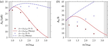
Figure 11. Comparisons between the asymptotic theory and the Navier–Stokes simulations, showing the variation of initial TS wave amplitude as a function of frequency: (a) acoustic wave receptivity, (b) vibrating ribbon receptivity. The grey areas delimit the range of unstable frequencies as predicted by LST.
Finally, the variation of TS wave amplitude as a function of roughness height
 $h$
for cases M0.2E and M0.2A1 is compared with the linear asymptotic theory result in figure 12. The plot shows numerical results for two different Reynolds numbers, namely
$h$
for cases M0.2E and M0.2A1 is compared with the linear asymptotic theory result in figure 12. The plot shows numerical results for two different Reynolds numbers, namely
 $\mathit{Re}=1.0\times 10^{6}$
(case M0.2E) and
$\mathit{Re}=1.0\times 10^{6}$
(case M0.2E) and
 $\mathit{Re}=35.1\times 10^{6}$
(case M0.2A1). Note that, having normalised
$\mathit{Re}=35.1\times 10^{6}$
(case M0.2A1). Note that, having normalised
 $A_{0}$
using
$A_{0}$
using
 $\mathit{Re}^{1/2}$
, the theoretical result becomes independent of Reynolds number. The figure clearly shows that for
$\mathit{Re}^{1/2}$
, the theoretical result becomes independent of Reynolds number. The figure clearly shows that for
 $h/{\it\delta}_{99}<0.06$
, where
$h/{\it\delta}_{99}<0.06$
, where
 ${\it\delta}_{99}$
is the boundary-layer thickness at the centre of the roughness element, the numerical results follow closely the linear behaviour predicted by the asymptotic theory. On the other hand, the discrepancy between theoretical and numerical results increases rather quickly starting from
${\it\delta}_{99}$
is the boundary-layer thickness at the centre of the roughness element, the numerical results follow closely the linear behaviour predicted by the asymptotic theory. On the other hand, the discrepancy between theoretical and numerical results increases rather quickly starting from
 $h/{\it\delta}_{99}\approx 0.06$
, indicating that nonlinear effects start becoming important for
$h/{\it\delta}_{99}\approx 0.06$
, indicating that nonlinear effects start becoming important for
 $h\approx 0.06{\it\delta}_{99}$
(or
$h\approx 0.06{\it\delta}_{99}$
(or
 $h\approx 0.17{\it\delta}^{\ast }$
). This result is in very good agreement with that reported by Choudhari & Street (Reference Choudhari and Street1992) and Crouch (Reference Crouch1992) when comparing their finite-Reynolds-number Orr–Sommerfeld receptivity theory results with the experiments of Saric, Hoos & Radeztsky (Reference Saric, Hoos, Radeztsky, Reda, Reed and Kobayashi1991), which were carried out for a Reynolds number of
$h\approx 0.17{\it\delta}^{\ast }$
). This result is in very good agreement with that reported by Choudhari & Street (Reference Choudhari and Street1992) and Crouch (Reference Crouch1992) when comparing their finite-Reynolds-number Orr–Sommerfeld receptivity theory results with the experiments of Saric, Hoos & Radeztsky (Reference Saric, Hoos, Radeztsky, Reda, Reed and Kobayashi1991), which were carried out for a Reynolds number of
 $\mathit{Re}=3.39\times 10^{5}$
. Interestingly, these results suggest that the critical value of
$\mathit{Re}=3.39\times 10^{5}$
. Interestingly, these results suggest that the critical value of
 $h/{\it\delta}_{99}$
, needed for nonlinear receptivity, is little affected by the Reynolds number.
$h/{\it\delta}_{99}$
, needed for nonlinear receptivity, is little affected by the Reynolds number.

Figure 12. Comparison between the asymptotic theory and the Navier–Stokes simulations for the acoustic wave receptivity study, showing the variation of initial TS wave amplitude as a function of roughness height.
6. Conclusions
The receptivity of Tollmien–Schlichting waves in subsonic boundary layers has been investigated using triple-deck theory and numerical simulations of the compressible Navier–Stokes equations. The investigation focused on the two receptivity problems arising due to the interaction between an acoustic wave and a small isolated roughness element placed on the wall of a flat plate, and due to the time-periodic vibrations of a ribbon placed on the wall of an otherwise smooth flat plate. A parametric study looking at the effects of roughness element and vibrating ribbon longitudinal dimensions, Reynolds number and Mach number was performed in order to thoroughly investigate the accuracy of the asymptotic theory for the prediction of lower-branch TS wave receptivity in subsonic boundary layers.
The results show that the theoretical predictions are in good agreement with the Navier–Stokes results. For both the receptivity problems analysed, the amplitude
 $A_{0}$
of the excited TS wave was found to be dependent on the Fourier transform of the wall disturbance (i.e. the roughness element or the vibrating ribbon) rather than being directly affected by its shape. In particular, only the Fourier coefficient corresponding to the TS wave wavenumber is responsible for the receptivity process. In the case of the TS wave receptivity due to sound, both the theoretical and numerical results indicate that the TS wave amplitude increases with Reynolds number proportionally to
$A_{0}$
of the excited TS wave was found to be dependent on the Fourier transform of the wall disturbance (i.e. the roughness element or the vibrating ribbon) rather than being directly affected by its shape. In particular, only the Fourier coefficient corresponding to the TS wave wavenumber is responsible for the receptivity process. In the case of the TS wave receptivity due to sound, both the theoretical and numerical results indicate that the TS wave amplitude increases with Reynolds number proportionally to
 $\mathit{Re}^{1/2}$
. In this case the agreement between theory and Navier–Stokes simulations is excellent. Despite the theoretical results being derived for large values of the Reynolds number, the numerical simulations show that the theory performs well for Reynolds numbers down to at least
$\mathit{Re}^{1/2}$
. In this case the agreement between theory and Navier–Stokes simulations is excellent. Despite the theoretical results being derived for large values of the Reynolds number, the numerical simulations show that the theory performs well for Reynolds numbers down to at least
 $\mathit{Re}=1.0\times 10^{5}$
; the relative error between theory and numerical simulations was found to be approximately
$\mathit{Re}=1.0\times 10^{5}$
; the relative error between theory and numerical simulations was found to be approximately
 $7\,\%$
of the theoretical result for Reynolds numbers between 1.0 × 10⁵ and 35.1 × 10⁶ at
$7\,\%$
of the theoretical result for Reynolds numbers between 1.0 × 10⁵ and 35.1 × 10⁶ at
 $\mathit{Ma}=0.2$
. As the Mach number increases, the TS wave receptivity is enhanced mainly due to the higher near-wall
$\mathit{Ma}=0.2$
. As the Mach number increases, the TS wave receptivity is enhanced mainly due to the higher near-wall
 $u$
velocity disturbances induced by the acoustic wave at higher free-stream Mach numbers. The asymptotic theory suggests that the TS wave amplitude increases according to
$u$
velocity disturbances induced by the acoustic wave at higher free-stream Mach numbers. The asymptotic theory suggests that the TS wave amplitude increases according to
 $A_{0}/(ah)\propto (\mathit{Ma}/(1+\mathit{Ma})){\it\lambda}(\mathit{Ma})$
, which agrees qualitatively with the numerical results obtained for both
$A_{0}/(ah)\propto (\mathit{Ma}/(1+\mathit{Ma})){\it\lambda}(\mathit{Ma})$
, which agrees qualitatively with the numerical results obtained for both
 $\mathit{Re}=8.4\times 10^{6}$
and
$\mathit{Re}=8.4\times 10^{6}$
and
 $\mathit{Re}=35.1\times 10^{6}$
. However, the relative error increases slightly for increasing Mach number, reaching a maximum of approximately 13.5 % at
$\mathit{Re}=35.1\times 10^{6}$
. However, the relative error increases slightly for increasing Mach number, reaching a maximum of approximately 13.5 % at
 $\mathit{Ma}=0.8$
.
$\mathit{Ma}=0.8$
.
The results obtained for the vibrating ribbon receptivity problem indicate that the amplitude of the excited TS wave is proportional to
 $\mathit{Re}^{3/8}$
. In this case the relative error between theory and Navier–Stokes simulations is approximately 23 % of the theoretical result and remains nearly constant for Reynolds numbers between 1.0 × 10⁵ and 35.1 × 10⁶ at
$\mathit{Re}^{3/8}$
. In this case the relative error between theory and Navier–Stokes simulations is approximately 23 % of the theoretical result and remains nearly constant for Reynolds numbers between 1.0 × 10⁵ and 35.1 × 10⁶ at
 $\mathit{Ma}=0.2$
. The agreement between theory and Navier–Stokes simulations remains good also in this case, especially considering that the theoretical results were derived by keeping only the leading-order terms in the asymptotic expansions. When looking at how the receptivity varies with Mach number, it was found that, while the numerical simulations show that the TS wave amplitude decreases as the Mach number increases, the theoretically predicted wall pressure presents a singularity for
$\mathit{Ma}=0.2$
. The agreement between theory and Navier–Stokes simulations remains good also in this case, especially considering that the theoretical results were derived by keeping only the leading-order terms in the asymptotic expansions. When looking at how the receptivity varies with Mach number, it was found that, while the numerical simulations show that the TS wave amplitude decreases as the Mach number increases, the theoretically predicted wall pressure presents a singularity for
 $\mathit{Ma}=1$
and, as a consequence, numerical and theoretical results quickly depart from each other as
$\mathit{Ma}=1$
and, as a consequence, numerical and theoretical results quickly depart from each other as
 $\mathit{Ma}\rightarrow 1$
. The singularity appears in the form of the factor
$\mathit{Ma}\rightarrow 1$
. The singularity appears in the form of the factor
 ${\it\beta}^{-1/4}$
and originates in the upper deck. Despite this singularity, it was found that the amplitude variation with Mach number extracted from the numerical results follows closely that obtained from the theoretical result after neglecting the contribution from
${\it\beta}^{-1/4}$
and originates in the upper deck. Despite this singularity, it was found that the amplitude variation with Mach number extracted from the numerical results follows closely that obtained from the theoretical result after neglecting the contribution from
 ${\it\beta}$
to the pressure disturbance at the wall, so that the TS wave amplitude varies as
${\it\beta}$
to the pressure disturbance at the wall, so that the TS wave amplitude varies as
 $A_{0}/h\propto {\it\mu}_{w}^{1/4}(\mathit{Ma}){\it\rho}_{w}^{1/2}(\mathit{Ma}){\it\lambda}^{5/4}(\mathit{Ma})$
.
$A_{0}/h\propto {\it\mu}_{w}^{1/4}(\mathit{Ma}){\it\rho}_{w}^{1/2}(\mathit{Ma}){\it\lambda}^{5/4}(\mathit{Ma})$
.
Additional numerical simulations indicate that the asymptotic theory can also be used to predict the receptivity of unstable TS waves with good accuracy. In addition, in agreement with the findings of Choudhari & Street (Reference Choudhari and Street1992) and Crouch (Reference Crouch1992), we show that the receptivity process due to the acoustic wave–roughness interaction is linear provided the height of the roughness element is smaller than approximately 6 % of the local boundary-layer thickness.
The theoretical triple-deck results are obtained under several assumptions regarding the order of magnitude of the size, amplitude and frequency of the external disturbances. These assumptions are needed in order to arrive at the asymptotic solutions for large values of the Reynolds number. However, the numerical results presented in this work show that the behaviour of the solutions obtained for
 $\mathit{Re}\rightarrow \infty$
holds also for finite Reynolds numbers and, in practice, the only conditions to be met in order for the theory to give reliable predictions are that the amplitude of the disturbances considered (acoustic wave, roughness element and vibrating ribbon for the cases analysed here) be small enough for the receptivity process to be linear and that the free-stream Mach number be subsonic. As such, it appears clear that the asymptotic theory of receptivity represents a good candidate for providing the amplitude information missing in current laminar–turbulent transition prediction methods.
$\mathit{Re}\rightarrow \infty$
holds also for finite Reynolds numbers and, in practice, the only conditions to be met in order for the theory to give reliable predictions are that the amplitude of the disturbances considered (acoustic wave, roughness element and vibrating ribbon for the cases analysed here) be small enough for the receptivity process to be linear and that the free-stream Mach number be subsonic. As such, it appears clear that the asymptotic theory of receptivity represents a good candidate for providing the amplitude information missing in current laminar–turbulent transition prediction methods.
Acknowledgements
This research was performed in the Laminar Flow Control Centre (LFC-UK) at Imperial College London. The Centre is supported by EPSRC, Airbus UK and EADS Innovation Works. The numerical simulations were performed in the Imperial College cx1 cluster. The authors would like to thank Professor Neil D. Sandham for providing the SBLI code used for the numerical study and the anonymous referees for their constructive comments.


