


1. Introduction
At supersonic speeds, the swept-wing leading edge is subject to high thermal loads. To facilitate the leading-edge thermal protection, it is required to predict and, if feasible, avoid the laminar–turbulent transition leading to a significant increase of aerodynamic heating.
If the swept leading edge is smooth and it is not contaminated by free-stream disturbances, transition follows the low-disturbance scenario including the three major stages (Morkovin, Reshotko & Herbert Reference Morkovin, Reshotko and Herbert1994): excitation of unstable modes of small initial amplitude (receptivity stage), spatial growth of instability along the attachment line (amplification stage governed by the linear stability theory) and nonlinear breakdown leading to a turbulent boundary-layer flow. Low-speed experiments (see Poll Reference Poll1979) showed that this scenario is relevant to the case where transition is observed at the Reynolds number  $R \equiv W_e^\ast {\varDelta ^\ast }/\nu _e^\ast\approx 650$. Hereafter,
  ${\varDelta ^\ast } = (\nu _e^\ast{/}\textrm{d}U_e^\ast{/}\textrm{d}{x^\ast })_{{x^\ast } = 0}^{1/2}$ is a characteristic length scale associated with the boundary-layer thickness, the upper asterisk denotes dimensional quantities, and the subscript ‘e’ denotes quantities at the upper boundary-layer edge. The flow scheme and notations are shown in figure 1. In the range
  $250 < R < 650$, transition is sensitive to the leading-edge roughness, free-stream disturbances and other external forcing, which trigger early nonlinear breakdown with partial or complete bypass of the linear amplification stage. For
  $R \le 250$, the contaminated attachment-line flow is relaminarised: initial disturbances decay and the laminar flow sets in again.
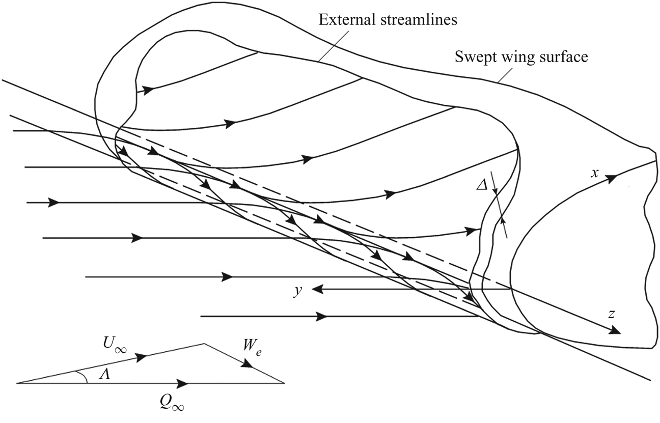
Figure 1. Flow scheme and notation.
Review of similar experiments at supersonic speeds is given by Lin & Malik (Reference Lin and Malik1995), see also Benard, Sidorenko & Raghunathan (Reference Benard, Sidorenko and Raghunathan2002). Analysing these data, Poll (Reference Poll1994) introduced the reduced Reynolds number  ${R_\ast } \equiv W_e^\ast {\varDelta ^\ast }({\nu ^\ast })/{\nu ^\ast }$, where the kinematic viscosity
  ${\nu ^\ast }$ is calculated at the reference temperature
 \begin{equation}T_\ast ^\ast = T_e^\ast + 0.1(T_w^\ast - T_e^\ast ) + 0.6(T_r^\ast - T_e^\ast ),\end{equation}
where  $T_r^\ast = T_e^\ast (1 + \sqrt {Pr} ((\gamma - 1)/2)M_e^2)\; $ is the recovery temperature,
  ${M_e} = W_e^\ast{/}a_e^\ast $ is the local Mach number and the subscript ‘w’ denotes quantities on the wall surface.
However, the low disturbance environment criterion  ${R_{{\ast} tr}} \approx 650$ poorly correlates with transition data obtained on smooth swept cylinders at large sweep Mach numbers. Namely, in the wind-tunnel experiments of Gaillard, Benard & Alziary de Roquefort (Reference Gaillard, Benard and Alziary de Roquefort1999) for
  ${M_e} > 4$, the transition onset Reynolds number decreases with
  ${M_e}$ and for
  ${M_e} > 6$, approaches the contamination level
  ${R_{{\ast} tr}} = 250$.
Xi, Ren & Fu (Reference Xi, Ren and Fu2021) recently performed a numerical study of the attachment-line instability for the conditions relevant to the experiments of Gaillard et al. (Reference Gaillard, Benard and Alziary de Roquefort1999). Using the Navier–Stokes (N-S) mean flow on a swept cylinder, they carried out stability analysis based on two-dimensional partial differential equations (2-D PDE). It was shown that, in the relatively low speed region  $({M_e} < 4)$, the attachment-line modes can be treated as an extension of Tollmien–Schlichting (TS) modes (Lin & Malik Reference Lin and Malik1995), while in the high speed region
  $({M_e} > 4)$, the attachment-line modes are closer to the Mack modes (Mack Reference Mack1975) of the inviscid nature. The behaviour of the Mack-like modes explains why the critical transition Reynolds number decreases as the sweep Mach number increases in the experiment of Gaillard et al. (Reference Gaillard, Benard and Alziary de Roquefort1999).
However, Xi et al. (Reference Xi, Ren and Fu2021) did not show detailed point-by-point comparisons with the transition data. It is not clear under what conditions the Mack-like modes compete with the TS-like modes and become dominant. Moreover, we found that the N-S mean flow solutions, which were used by Xi et al. (Reference Xi, Ren and Fu2021) in their stability analyses, do not agree with our N-S solutions and the compressible Hiemenz solution, which casts doubt on the correctness of the results reported.
To clarify this situation, we conduct a broadband parametric study, which is difficult to perform using the computationally expensive 2-D PDE approach of Xi et al. (Reference Xi, Ren and Fu2021). We put together and employed the following theoretical model: (1) the mean-flow parameters at the upper boundary-layer edge are calculated using the inviscid theory of Rechotko & Beckwith (Reference Rechotko and Beckwith1958); (2) the boundary-layer profiles are computed using the compressible Hiemenz solution (Pfenninger Reference Pfenninger1965, Gaster Reference Gaster1967); (3) the stability problem, which describes discrete modes propagating in the laminar attachment-line boundary layer, is solved using the theoretical model of Theofilis, Fedorov & Collis (Reference Theofilis, Fedorov and Collis2006), see also Semisynov et al. (Reference Semisynov, Fedorov, Novikov, Semionov and Kosinov2003). The model is based on successive approximation procedures of the type formulated independently by Gaster (Reference Gaster1974) and Bouthier (Reference Bouthier1972, Reference Bouthier1973).
This approach is based on the following findings. In the low-speed cases (incompressible flow), the Hiemenz solution agrees well with the mean flow measurements of Gaster (Reference Gaster1967) and Poll (Reference Poll1979). The temporal stability of the incompressible Hiemenz flow was analysed by Hall, Malik & Poll (Reference Hall, Malik and Poll1984) with the assumption that the unstable mode (hereafter, HMP mode) is symmetric and its chordwise velocity is a linear function of the  $x$-coordinate. Hall & Malik (Reference Hall and Malik1986) analysed weakly nonlinear effects associated with the HMP mode. They showed that, apart from a small interval near the (linear) critical Reynolds number, finite-amplitude solutions bifurcate subcritically from the upper branch of the neutral curve. Both the weakly nonlinear theory and the numerical calculations showed the existence of supercritical finite-amplitude (equilibrium) states near the lower branch, which explains why the observed flow exhibits a preference for the lower branch modes. The direct numerical simulation of Spalart (Reference Spalart1988) gave support to the use of the HMP ansatz. Balakumar & Trivedi (Reference Balakumar and Trivedi1998) obtained 2-D nonlinear equilibrium solutions by solving the full Navier–Stokes equations as a nonlinear eigenvalue problem. The behaviour of these solutions is consistent with the weakly nonlinear theory. Their secondary instability was investigated using the Floquet theory. The results showed that these 2-D finite amplitude neutral solutions are unstable to three-dimensional (3-D) disturbances.
Lin & Malik (Reference Lin and Malik1996) solved the 2-D PDE eigenvalue problem and found symmetric (Sj) and antisymmetric (Aj) discrete modes of the type  $f(x,y){\rm exp} (\textrm{i}\beta z - \textrm{i}\omega t)$, where
  $\omega (\beta ) = {\omega _r}(\beta ) + \textrm{i}{\omega _i}(\beta )$ is complex eigenvalue and
  $j = 1,\; 2, \ldots $ Computations showed that the HMP mode corresponds to the symmetric mode S 1 having the highest growth rate
  ${\omega _i}$.
Theofilis et al. (Reference Theofilis, Fedorov, Obrist and Dallman2003) found that eigenmodes of the 2-D-PDE stability problem have a polynomial structure versus x and the 2-D eigenvalue problem can be reduced to a system of one-dimensional (1-D) problems of the Orr–Sommerfeld class. Using the successive approximation procedure of Gaster (Reference Gaster1974), they derived a compact semi-analytical relationship providing quick computations of the eigenvalues  $\omega $ for modes Sj and Aj. Theofilis et al. (Reference Theofilis, Fedorov and Collis2006) demonstrated that a similar relationship is valid for compressible attachment-line flows, albeit restricted to certain ranges of Reynolds number owing to the error of the second-order asymptotic terms scaled as
  $O(M_e^2/{R^2})$. Considering the stability of the compressible Hiemenz flows at
  ${M_e} = 0.5$ and 0.9, Gennaro et al. (Reference Gennaro, Rodríguez, Medeiros and Theofilis2013) obtained perfect agreement between the temporal growth rates
  ${\omega _i}$ of mode S 1 predicted by solving the 2-D-PDE stability problem and using the 1-D theoretical analysis.
In addition to reconsidering the cases reported by Xi et al. (Reference Xi, Ren and Fu2021) and correcting their results, this paper suggests a theoretical model, which captures the attachment-line modes and allows us to determine regions of their dominance in the  ${M_e} - {T_f}$ space. This model helps to perform quick parametric studies of the compressible attachment-line instability, shed light on the mechanisms of instability and extrapolate the knowledge gained on the supersonic boundary layer stability to the attachment-line flow.
The rest of this paper is organised as follows. In § 2, we discuss the methodology and compare the theoretical growth rates of the most unstable mode with those resulting from the 2-D-PDE stability computations of Li & Choudhari (Reference Li and Choudhari2008) in the case of  ${M_e} = 1.69$. In § 3, parametric stability computations are performed to identify regions where one or another unstable mode is dominant. It will be shown that at sufficiently high
  ${M_e}$ and low wall-temperature ratio
  ${T_f} \equiv T_w^\mathrm{\ast }/T_r^\mathrm{\ast }$, the attachment-line flow can support discrete modes of acoustic nature. The most unstable among them is similar to the Mack second mode in the flat-plate boundary layer. In § 4, we analyse experimental data reported by Gaillard et al. (Reference Gaillard, Benard and Alziary de Roquefort1999) with emphasis on high local Mach numbers
  $({M_e} > 4)$ associated with large angles of the leading-edge sweep. The results are summarised in § 5.
2. Methodology
2.1. Mean flow
Consider the near-wall compressible laminar flow on a swept cylinder of radius  ${r^\mathrm{\ast }}$ and infinite length in the spanwise direction z (figure 1). In this case, the flow field does not depend on z. Gas is perfect with constant specific heat ratio
  $\gamma $ and Prandtl number Pr. The dimensionless viscosity
  $\mu = {\mu ^\mathrm{\ast }}/\mu _e^\mathrm{\ast }$ is approximated by the power law
  $\mu (T) = {T^m}$ or the Sutherland law
  $\mu = {T^{3/2}}(1 + S)/(T + S),\;S = 110.4K/T_e^\ast $.
In the attachment line vicinity, the near-wall flow can be described by the compressible Hiemenz solution (Theofilis et al. Reference Theofilis, Fedorov and Collis2006). For small values of  ${\varDelta ^\mathrm{\ast }}/{r^\mathrm{\ast }}$, the cylinder-surface curvature can be neglected. Then, the coordinate system
  $(x,y,z) = ({x^\mathrm{\ast }},{y^\mathrm{\ast }},{z^\mathrm{\ast }})/{\varDelta ^\mathrm{\ast }}$ is locally Cartesian. The velocity components
  $({u^\mathrm{\ast }},{v^\mathrm{\ast }},{w^\mathrm{\ast }})$, temperature
  ${T^\mathrm{\ast }}$ and pressure
  ${P^\mathrm{\ast }}$ are scaled using
  $W_e^\mathrm{\ast }$,
  $T_e^\mathrm{\ast }$ and
  $\rho _e^\mathrm{\ast }W_e^{\mathrm{\ast }2}$, where the flow parameters at the upper boundary-layer edge are calculated using the analytical relations derived by Rechotko & Beckwith (Reference Rechotko and Beckwith1958).
In the attachment line vicinity,
 \begin{equation}(u,v,w) = (\varepsilon xU(y),\varepsilon V(y),W(y)),\quad T = T(y),\quad P = {(\gamma M_e^2)^{ - 1}} - {\varepsilon ^2}{x^2}/2,\end{equation}
where  $\varepsilon = {R^{ - 1}}$ is assumed to be small. The mean-flow profiles
  $U(y),V(y),W(y),T(y)$ are governed by the ordinary differential equation (ODE) system
 \begin{equation}\left.
{\begin{gathered} {({U^2} + VU^{\prime})/T = 1 +
\mu^{\prime}T^{\prime}U^{\prime} + \mu U^{\prime\prime}}\\
{VW^{\prime}/T = \mu^{\prime}T^{\prime}W^{\prime} + \mu
W^{\prime\prime}}\\ {U - VT^{\prime}/T + V^{\prime} = 0}\\
{(\mu^{\prime}{{T^{\prime}}^2} + \mu T^{\prime\prime})/Pr -
T^{\prime}V/T + M_e^2(\gamma - 1)\mu {{W^{\prime}}^2} = 0}
\end{gathered}} \right\},\end{equation}
\begin{equation}\left.
{\begin{gathered} {({U^2} + VU^{\prime})/T = 1 +
\mu^{\prime}T^{\prime}U^{\prime} + \mu U^{\prime\prime}}\\
{VW^{\prime}/T = \mu^{\prime}T^{\prime}W^{\prime} + \mu
W^{\prime\prime}}\\ {U - VT^{\prime}/T + V^{\prime} = 0}\\
{(\mu^{\prime}{{T^{\prime}}^2} + \mu T^{\prime\prime})/Pr -
T^{\prime}V/T + M_e^2(\gamma - 1)\mu {{W^{\prime}}^2} = 0}
\end{gathered}} \right\},\end{equation}
with the boundary conditions
 \begin{equation}\left.
{\begin{gathered} {y = 0:\;U = V = W = 0}\\ {T =
{T_w}\;\textrm{for}\;\textrm{isothermal}\;\textrm{wall},\;\textrm{or}\;T^{\prime}
=
0\;\textrm{for}\;\textrm{thermally}\;\textrm{isolated}\;\textrm{wall}}\\
{y = \infty :\;U = W = T = 1} \end{gathered}}
\right\}.\end{equation}
\begin{equation}\left.
{\begin{gathered} {y = 0:\;U = V = W = 0}\\ {T =
{T_w}\;\textrm{for}\;\textrm{isothermal}\;\textrm{wall},\;\textrm{or}\;T^{\prime}
=
0\;\textrm{for}\;\textrm{thermally}\;\textrm{isolated}\;\textrm{wall}}\\
{y = \infty :\;U = W = T = 1} \end{gathered}}
\right\}.\end{equation}
Note that for incompressible flows, the Hiemenz solution is an exact Navier–Stokes solution. For compressible flows, this is not the case owing to the error of the order of  $O({\varepsilon ^2}M_e^2)$. The system (2.2) is integrated numerically using the fourth-order Runge–Kutta algorithm. More than 400 grid points equally spaced versus y are needed to compute the boundary-layer profiles with six significant digits.
In addition, the laminar flow past a swept cylinder is calculated using the in-house N-S solver. The 2-D computational domain is limited by: the detached bow shock with the Rankine–Hugoniot conditions; the body surface with no-slip and isothermal boundary conditions; the symmetry line; and the chordwise edge, which corresponds to the azimuthal angle  ${\rm \pi}/2$, with the soft boundary condition – the linear extrapolation of dependant variables.
The problem is solved numerically using the method of bow-shock isolation (Egorov Reference Egorov1992). For approximation of convective and diffusion components of the flow vector in semi-integer nodes on the elementary cell edges, the second-order central difference scheme on a nine-point “box” stencil is used. This scheme does not belong to the family of monotone difference schemes and, therefore, cannot be used for solving problems with discontinuities. However, in the case where dependant variables are smooth and the physical dissipation is present, central difference schemes allow us to obtain more accurate solutions compared with monotone schemes on the same computational grids. To solve the nonlinear difference equations approximating the differential equations, the modified Newton–Raphson method is used. The system of linear algebraic equations obtained at each iteration step, is solved using the direct method of LU-decomposition with preliminary renumbering of unknowns by the nested dissection method.
Computations are performed on a non-uniform computational grid containing 201 nodes along the cylinder surface and 301 nodes in the wall normal direction. Near the shock wave and the body surface there are thin layers, which contain, after clustering, approximately 10 % and 55 % of the total number of nodes, respectively.
Figure 2 compares the theoretical and N-S mean-flow solutions for the case C3373a specified in table 2 of Appendix A. The profiles  $U(y),W(y),T(y)$ and their derivatives agree very well. The discrepancy in
  $V(y)$ is not appreciable, because the vertical velocity
  $\varepsilon V(y)$ is not involved into the leading-order approximation of the eigenvalue problem for disturbances (see § 2.2).

Figure 2. The mean flow profiles in case C3373a: lines, compressible Hiemenz solution; symbols, our N-S solution.
This result disagrees with similar comparisons reported by Xi et al. (Reference Xi, Ren and Fu2021). Namely, the N-S mean-flow profiles differ significantly from the boundary layer approximation. As shown in Appendix B, the N-S mean-flow solutions of Xi et al. (Reference Xi, Ren and Fu2021) are not correct. This led to the wrong conclusion: “the traditional boundary layer model fails to take the influence of inviscid flow into consideration this influence sometimes may change the physics of flow instability significantly…”
2.2. Stability analysis
The disturbance vector is expressed as
 \begin{equation}\boldsymbol{q}(x,y,z,t) \equiv {\left( {u,\frac{{\partial u}}{{\partial y}},v,p,\theta ,\frac{{\partial \theta }}{{\partial y}},w,\frac{{\partial w}}{{\partial y}}} \right)^T} = \boldsymbol{F}(x,y)\textrm{exp[i}(\beta z - \omega t)\textrm{]},\end{equation}
where  $t = {t^\mathrm{\ast }}W_e^\mathrm{\ast }/{\varDelta ^\mathrm{\ast }}$ is time and
  $\theta $ is non-dimensional temperature. Because the attachment-line flow is convectively unstable, we consider the spatial stability problem, where
  $\omega $ is real and
  $\beta $ is a complex eigenvalue with
  $\sigma ={-} {\beta _i}$ representing the growth rate of a wave propagating along the attachment line.
For quasi-2-D disturbances, the vector-function  $\boldsymbol{F}$ is expanded as (Theofilis et al. Reference Theofilis, Fedorov and Collis2006)
 \begin{equation}\boldsymbol{F} = {\boldsymbol{Z}_0}(y;{x_1},{z_1}) + \varepsilon {\boldsymbol{Z}_1}(y;{x_1},{z_1}) + \cdots ,\end{equation}
where  ${x_1} = \varepsilon x$ and
  ${z_1} = \varepsilon z$ are slow variables. In accord with the Gaster (Reference Gaster1974) approach (see also Nayfeh Reference Nayfeh1980) the zero-order term is expressed as
  ${\boldsymbol{Z}_0} = C({x_1},{z_1})\boldsymbol{\xi }(y,{x_1})$, where
  $\boldsymbol{\xi }$ is solution of the problem
 \begin{equation}\left.
{\begin{gathered} {\dfrac{{\partial \boldsymbol{\xi
}}}{{\partial y}} = \boldsymbol{A\xi }}\\ {{\xi_1} =
{\xi_3} = {\xi_5} = {\xi_7} = 0,\quad y = 0}\\ {{\xi_1} =
{\xi_3} = {\xi_5} = {\xi_7} = 0,\quad y = \infty }
\end{gathered}} \right\},\end{equation}
\begin{equation}\left.
{\begin{gathered} {\dfrac{{\partial \boldsymbol{\xi
}}}{{\partial y}} = \boldsymbol{A\xi }}\\ {{\xi_1} =
{\xi_3} = {\xi_5} = {\xi_7} = 0,\quad y = 0}\\ {{\xi_1} =
{\xi_3} = {\xi_5} = {\xi_7} = 0,\quad y = \infty }
\end{gathered}} \right\},\end{equation}
which delivers the eigenvalue  $\beta = {\beta _0}(\omega ,R)$. Here
  $\boldsymbol{A}$ is an 8 × 8 matrix of the linear stability problem. Its explicit form can be found in Mack (Reference Mack1979), Nayfeh (Reference Nayfeh1980), Tumin (Reference Tumin2007) and other papers. Note that some elements of this matrix include
  $\varepsilon $ and therefore (2.5) is not a self-consistent asymptotic expansion. Nevertheless, Tumin (Reference Tumin2006) showed that this inconsistency does not lead to an erroneous asymptotic behaviour of Tollmien–Schlichting waves. Numerous papers demonstrated robustness of this approach to receptivity and stability problems for weakly non-parallel compressible boundary-layer flows (for example, see the survey of Tumin Reference Tumin2011).
For the compressible Hiemenz flow,  ${\beta _0}$ does not depend on
  ${x_1}$ while the eigenvector
  $\boldsymbol{\xi }$ can be expressed in the form
 \begin{equation}\boldsymbol{\xi }({x_1},y) = {({x_1}{\xi _{01}}(y),{x_1}{\xi _{02}}(y),{\xi _{03}}(y),{\xi _{04}}(y),{\xi _{05}}(y),{\xi _{06}}(y),{\xi _{07}}(y),{\xi _{08}}(y))^T}.\end{equation}
In the first-order approximation, we obtain the inhomogeneous problem
 \begin{equation}\left.
{\begin{gathered} {\dfrac{{\partial
{\boldsymbol{Z}_1}}}{{\partial y}} = \boldsymbol{A}{\boldsymbol{Z}_1} +
{\boldsymbol{G}_x}\dfrac{{\partial
{\boldsymbol{Z}_0}}}{{\partial {x_1}}} +
{\boldsymbol{G}_z}\dfrac{{\partial
{\boldsymbol{Z}_0}}}{{\partial {z_1}}} +
\boldsymbol{H}{\boldsymbol{Z}_0}}\\ {{Z_{11}} = {Z_{13}} =
{Z_{15}} = {Z_{17}} = 0,\quad y = 0}\\ {{Z_{11}} = {Z_{13}}
= {Z_{15}} = {Z_{17}} = 0,\quad y = \infty } \end{gathered}}
\right\},\end{equation}
\begin{equation}\left.
{\begin{gathered} {\dfrac{{\partial
{\boldsymbol{Z}_1}}}{{\partial y}} = \boldsymbol{A}{\boldsymbol{Z}_1} +
{\boldsymbol{G}_x}\dfrac{{\partial
{\boldsymbol{Z}_0}}}{{\partial {x_1}}} +
{\boldsymbol{G}_z}\dfrac{{\partial
{\boldsymbol{Z}_0}}}{{\partial {z_1}}} +
\boldsymbol{H}{\boldsymbol{Z}_0}}\\ {{Z_{11}} = {Z_{13}} =
{Z_{15}} = {Z_{17}} = 0,\quad y = 0}\\ {{Z_{11}} = {Z_{13}}
= {Z_{15}} = {Z_{17}} = 0,\quad y = \infty } \end{gathered}}
\right\},\end{equation}
where  ${\boldsymbol{G}_z} ={-} \textrm{i}\partial \boldsymbol{A}/\partial \beta $,
  ${\boldsymbol{G}_x} ={-} \textrm{i}\partial \boldsymbol{A}/\partial \alpha $ and the matrix
  $\boldsymbol{H}$ depends on the mean-flow profiles
  $U(y)$ and
  $V(y)$.
The problem (2.8) has a non-trivial solution if the inhomogeneous part is orthogonal to the solution  $\boldsymbol{\zeta }$ of the adjoint problem. This leads to the equation for the amplitude function
  $C({x_1},{z_1})$
 \begin{equation}\langle {\boldsymbol{G}_x}\boldsymbol{\xi },\boldsymbol{\zeta }\rangle \frac{{\partial C}}{{\partial {x_1}}} + \langle {\boldsymbol{G}_z}\boldsymbol{\xi },\boldsymbol{\zeta }\rangle \frac{{\partial C}}{{\partial {z_1}}} + C\left[ {\left\langle {{\boldsymbol{G}_x}\frac{{\partial \boldsymbol{\xi }}}{{\partial {x_1}}},\boldsymbol{\zeta }} \right\rangle + \langle \boldsymbol{H\xi },\boldsymbol{\zeta }\rangle } \right] = 0,\end{equation}
where the scalar product is defined as  $\langle \boldsymbol{\xi },\boldsymbol{\zeta }\rangle = \int_0^\infty {(\sum\nolimits_{j,k = 1}^8 {{\xi _k}{\zeta _j}} )\,\textrm{d}y} $. Equation (2.9) can be written in a form similar to the incompressible case (Theofilis et al. Reference Theofilis, Fedorov, Obrist and Dallman2003)
 \begin{equation}{D_1}{x_1}\frac{{\partial C}}{{\partial {x_1}}} + {D_2}\frac{{\partial C}}{{\partial {z_1}}} + C{D_3} = 0,\end{equation}
where  ${D_{1,2,3}}$ are constants. Equation (2.10) admits the family of solutions
 \begin{equation}{C_n} = Bx_1^n\textrm{exp(i}{\beta _{1n}}{z_1}\textrm{),}\quad {\beta _{1n}} = i({D_3} + n{D_1})/{D_2},\end{equation}
where  $n = 0,1,2, \ldots $ and B is constant.
Thus, quasi-2-D modes can be expressed as
 \begin{equation}\left.
{\begin{gathered} {{\boldsymbol{q}_n}(x,y,z,t) =
Bx_1^n\boldsymbol{\xi }({x_1},y)[1 + O(\varepsilon
)]\textrm{exp[}i({\beta_n}z - \omega t)\textrm{]}}\\
{{\beta_n} = {\beta_0} + \varepsilon {\beta_{1n}} +
O({\varepsilon^2})} \end{gathered}}
\right\}.\end{equation}
\begin{equation}\left.
{\begin{gathered} {{\boldsymbol{q}_n}(x,y,z,t) =
Bx_1^n\boldsymbol{\xi }({x_1},y)[1 + O(\varepsilon
)]\textrm{exp[}i({\beta_n}z - \omega t)\textrm{]}}\\
{{\beta_n} = {\beta_0} + \varepsilon {\beta_{1n}} +
O({\varepsilon^2})} \end{gathered}}
\right\}.\end{equation}
Here  $n = 0,2, \ldots $ correspond to symmetric modes S 1, S 2,… and
  $n = 1,3, \ldots $ to antisymmetric modes A 1, A 2, … These modes are calculated using the following algorithm: (1) solve the zero-order problem (2.6) at
  ${x_1} = 0$, which is a standard stability problem for 2-D waves in a 2-D boundary layer with the mean-flow profiles
  $W(y)$ and
  $T(y)$; (2) solve the corresponding adjoint problem; (3) calculate the eigenvalues
  ${\beta _n}$ and the vector-functions
  ${\boldsymbol{q}_n}$ using (2.11) and (2.12).
For 3-D disturbances of the type
 \begin{equation}\boldsymbol{F} = [{\boldsymbol{Z}_0}(y;{x_1},{z_1}) + \varepsilon {\boldsymbol{Z}_1}(y;{x_1},{z_1}) + \cdots ]\textrm{exp(i}\alpha x\textrm{)},\end{equation}
the zeroth-order vector function is expressed as  ${\boldsymbol{Z}_0} = C({z_1})\boldsymbol{\xi }({x_1},y)$, where
  $\boldsymbol{\xi }$ is a solution of the eigenvalue problem (2.6) with the complex eigenvalue
  $\beta = {\beta _0}(\omega ,\alpha )$. In the first-order approximation,
  ${\boldsymbol{Z}_1}$ is a solution of the problem (2.8), while the amplitude coefficient is governed by the equation
 \begin{equation}\langle {\boldsymbol{G}_z}\boldsymbol{\xi },\boldsymbol{\zeta }\rangle \frac{{\partial C}}{{\partial {z_1}}} + C\left[ {\left\langle {{\boldsymbol{G}_x}\frac{{\partial \boldsymbol{\xi }}}{{\partial {x_1}}},\boldsymbol{\zeta }} \right\rangle + \langle \boldsymbol{H\xi },\boldsymbol{\zeta }\rangle } \right] = 0.\end{equation}
Its solution is
 \begin{equation}C = B {\rm exp} \textrm{(i}{\beta _1}{z_1}\textrm{)},\quad {\beta _1} = {{i\left[ {\left\langle {{\boldsymbol{G}_x}\frac{{\partial \boldsymbol{\xi }}}{{\partial {x_1}}},\boldsymbol{\zeta }} \right\rangle + \langle \boldsymbol{H\xi },\boldsymbol{\zeta }\rangle } \right]} / {\langle {\boldsymbol{G}_z}\boldsymbol{\xi },\boldsymbol{\zeta }\rangle }}.\end{equation}
In summary, the 3-D mode is expressed as
 \begin{equation}\left.
{\begin{gathered} {\boldsymbol{q}(x,y,z,t) =
B\boldsymbol{\xi }({x_1},y)[1 + O(\varepsilon )]{\rm exp}
[\textrm{i}(\alpha x + \beta z - \omega t)]}\\ {\beta =
{\beta_0} + \varepsilon {\beta_1} + O({\varepsilon^2})}
\end{gathered}}
\right\},\end{equation}
\begin{equation}\left.
{\begin{gathered} {\boldsymbol{q}(x,y,z,t) =
B\boldsymbol{\xi }({x_1},y)[1 + O(\varepsilon )]{\rm exp}
[\textrm{i}(\alpha x + \beta z - \omega t)]}\\ {\beta =
{\beta_0} + \varepsilon {\beta_1} + O({\varepsilon^2})}
\end{gathered}}
\right\},\end{equation}
Computations of quasi-2-D modes (2.12) and 3-D mode (2.16) are performed using an in-house linear stability solver. The fundamental solutions of the direct and adjoint eigenvalue problems are obtained by numerical integration of the equations from the upper boundary toward the wall with the known analytical asymptotic solutions outside the boundary layer using the Gramm–Schmidt orthonormalisation procedure and the fourth-order Runge–Kutta algorithm. Eigenfunctions of the direct and adjoint problems are expressed as a linear combination of the fundamental solutions, with coefficients being determined from the boundary conditions on the wall. To satisfy these conditions, the eigenvalues  $\beta $ are determined using the Newton–Raphson iterations.
The asymptotic solution (2.12) is validated by comparison with solutions of the 2-D-PDE stability problem reported by Li & Choudhari (Reference Li and Choudhari2008) for the compressible Hiemenz flow at  ${M_e} = 1.69$,
  $T_e^\mathrm{\ast } = 300\;\textrm{K}$,
  ${T_w} = {T_{ad}}$ (thermally isolated wall). Figure 3 shows that the theoretical growth rates
  $\sigma ={-} {\beta _i}(\omega )$ agree well with those predicted by the 2-D-PDE stability analysis for the first symmetric mode S 1. Similar comparisons for subsonic attachment-line flows (
 ${M_e} = 0.5$ and 0.9) were reported by Gennaro et al. (Reference Gennaro, Rodríguez, Medeiros and Theofilis2013).

Figure 3. Distributions  $\sigma ={-} {\beta _i}(\omega )$ of mode S 1 for the compressible Hiemenz flow at
  ${M_e} = 1.69$,
  $T_e^\mathrm{\ast } = 300\;\textrm{K}$,
  ${T_w} = {T_{ad}}$ and
  ${x_1} = 0$: lines, asymptotic solution (2.12); symbols, 2-D-PDE solution of Li & Choudhari (Reference Li and Choudhari2008).
Because the compressible Hiemenz mean-flow profiles agree well with the corresponding N-S profiles (figure 2), it is expected that stability characteristics of these flows also agree well. This is confirmed by figure 4 showing the maximal growth rates  ${\sigma _{max}}(R) = {\rm max}_\omega [ - {\beta _i}(\omega ,R)]$ of mode S 1 predicted by the theory in the case C3373a. A slight downward shift of
  ${\sigma _{max}}$ in the case of N-S mean flow seems to arise from the curvature effect.

Figure 4. Distribution of maximum growth rate  ${\sigma _{max}}(R)$ for mode S 1 in case C3373a.
For small  $\alpha :\alpha = a\varepsilon ,\;a = O(1)$, the factor
  $\textrm{exp(i}\alpha x\textrm{)}$ in (2.16) can be expanded in the Taylor series:
  $\textrm{exp(i}\alpha x\textrm{)} = \sum\nolimits_{n = 0}^\infty {{{(\textrm{i}a)}^n}x_1^n/n!} $, where
  $0! = 1$. Then the solution can be treated as a sum of symmetric
  $(n = 0,2, \ldots )$ and antisymmetric
  $(n = 1,3, \ldots )$ modes of the form (2.12). The dominant term of this expansion corresponds to
  $n = 0$. Consequently, in the attachment-line vicinity
  ${x_1} \ll 1$, the 3-D mode of (2.16) tends to the symmetric quasi-2-D mode S 1 as
  $\alpha \to 0$. This trend is illustrated in figure 5 for a supersonic attachment-line flow at
  ${M_e} = 1.55$,
  $T_e^\mathrm{\ast } = 300\;\textrm{K}$,
  ${T_w} = {T_{ad}}$, and in figure 6 for a hypersonic attachment-line flow at
  ${M_e} = 5$,
  $T_e^\mathrm{\ast } = 300\;\textrm{K}$,
  ${T_w} = 0.7{T_e}$. In the first case, the most unstable are oblique waves having the wave-front angle
  $\psi = \textrm{ta}{\textrm{n}^{ - 1}}(\alpha /{\beta _r}) \approx 42^\circ $. In the second case, the most unstable are plane waves of
  $\alpha = 0$.

Figure 5. Growth rate  $\sigma (\alpha )$ at
  $R = 1000$,
  $\omega = 0.0568$ and
  ${x_1} = 0$. The compressible Hiemenz mean flow at
  ${M_e} = 1.55$,
  $T_e^\mathrm{\ast } = 300\;\textrm{K}$,
  ${T_w} = {T_{ad}}$: line, 3-D mode (2.16); symbols, quasi-2-D modes (2.12);
  $\psi = \textrm{ta}{\textrm{n}^{ - 1}}(\alpha /{\beta _r})$, wave front angle.


This situation is similar to the case of boundary layer flow on a flat plate. For moderate supersonic speeds, the dominant attachment-line instability behaves as the TS-like first mode. It is natural to assume that for sufficiently large  ${M_e}$, the dominant instability is associated with the Mack second mode of acoustic nature. Indeed, figure 7 shows that there are fast and slow modes of the discrete spectrum. Owing to their synchronisation in the frequency band between the two vertical dashed lines, the slow mode becomes more unstable while the fast mode becomes more stable. This behaviour is in full accordance with the flat-plate case (see, for example, Fedorov Reference Fedorov2011 and Fedorov & Tumin Reference Fedorov and Tumin2011). Therefore, in what follows, we use the terminology of Mack for the dominant attachment-line instabilities. Further analysis is focused on the close vicinity of the attachment line and all computations are performed at
  ${x_1} = 0$.

Figure 7. Phase speeds  ${c_r}(\omega ) = {(\omega /\beta )_r}$ and the spatial decrements
  ${\beta _i}(\omega )$ of fast and slow modes at
  $R = 4000$ and
  $\alpha = 0$ for the compressible Hiemenz mean flow at
  ${M_e} = 5$,
  $T_e^\mathrm{\ast } = 300\;\textrm{K}$,
  ${T_w} = 5.308{T_e} \approx {T_{ad}}$ and
  ${x_1} = 0$: horizontal dashed lines, phase speeds of 2-D fast and slow acoustic waves of zero angle of incidence
  $({c_r} = 1 \pm 1/{M_e})$ and vortical/entropy waves
  $({c_r} = 1)$.
It should also be noted that the foregoing results contradict the statement of Xi et al. (Reference Xi, Ren and Fu2021) that the attachment-line mode associated with the Mack second mode is absent if the basic flow is calculated with boundary layer assumptions.
3. Parametric studies
Assume that the laminar–turbulent transition is associated with the spatial growth of unstable waves propagating along the attachment line. If the location of an instability source,  $z = {z_0}$, is known and the initial amplitudes of unstable waves weakly depend on frequency, the transition onset point,
  ${z_{tr}}$, is estimated as (Lin & Malik Reference Lin and Malik1995)
 \begin{equation}{N_{tr}} = {\sigma _{max}}({R_{tr}})({z_{tr}} - {z_0}),\end{equation}
where  ${\sigma _{max}}(R) = ma{x_{\omega ,\alpha }}[ - {\beta _i}(\omega ,\alpha ,R)]$, and
  ${N_{tr}}$ is the empirically determined N-factor. Usually,
  ${R_{tr}}$ is plotted as a function of
  ${z_{tr}} - {z_0}$ at a fixed value of
  ${N_{tr}}$ (Lin & Malik Reference Lin and Malik1995).
If  ${z_0}$ is unknown or receptivity is distributed along the attachment line, one can use the following conservative approach. In the vicinity of critical Reynolds number
  ${R_{cr}}:{\sigma _{max}}({R_{cr}}) = 0$, the growth rate is approximated as
  ${\sigma _{max}}(R) \approx (\textrm{d}{\sigma _{max}}/\textrm{d}R)({R_{cr}})(R - {R_{cr}})$. Substitution of this approximation into (3.1) gives
 \begin{equation}{R_{tr}} \approx
{R_{cr}}(1 + \delta ),\quad \delta =
\frac{{{N_{tr}}}}{{R\displaystyle\frac{{\textrm{d}\sigma
_{max}^\mathrm{\ast
}}}{{\textrm{d}R}}({R_{cr}})L_z^\mathrm{\ast
}}},\end{equation}
\begin{equation}{R_{tr}} \approx
{R_{cr}}(1 + \delta ),\quad \delta =
\frac{{{N_{tr}}}}{{R\displaystyle\frac{{\textrm{d}\sigma
_{max}^\mathrm{\ast
}}}{{\textrm{d}R}}({R_{cr}})L_z^\mathrm{\ast
}}},\end{equation}
where  $\sigma _{max}^\mathrm{\ast }$ is the dimensional growth rate and
  $L_z^\mathrm{\ast }$ is the leading-edge spanwise scale. In the majority of practical cases,
  $\delta \ll 1$, and the transition onset Reynolds number is estimated as
  ${R_{tr}} = {R_{cr}}$. This criterion indicates that at
  $R > {R_{tr}}$, transition occurs somewhere on a sufficiently long attachment line.
Consider air flow of  $\gamma = 1.4$ and Pr = 0.72 using the power law for the viscosity coefficient:
  $\mu (T) = {T^m}$. With this choice of the temperature–viscosity dependency, the mean-flow profiles (2.1a–c) are functions of the two parameters only: the local Mach number
  ${M_e}$ and the wall-temperature ratio
  ${T_f} = T_w^\mathrm{\ast }/T_r^\mathrm{\ast }$. Therefore, the power law is widely used in parametric studies. Depending on flow temperature, the exponent varies from
  $m = 1$ for relatively small T to
  $m = 0.7$ for high temperatures. Hereafter, we use
  $m = 0.75$. In § 4, it is shown that the critical Reynolds numbers predicted at this value of m are close to those in the case of the Sutherland law. Because the dominant attachment-line instability is captured by the asymptotic solution (2.16), further stability computations are performed using this solution only.
Figure 8 shows distributions of the reduced critical Reynolds number  ${R_{\mathrm{\ast }cr}}({T_f})$ at various values of
  ${M_e}$. The solid lines are relevant to 3-D waves of the first mode and the dashed lines refer to 2-D waves of the second mode. As an example, consider the case of
  ${M_e} = 4$ marked by arrows. In the region of small
  ${T_f}$, where the second mode is dominant,
  ${R_{\mathrm{\ast }cr}}$ monotonically increases with
  ${T_f}$ and reaches a value shown by the black circle. Starting from this point, the first mode takes over and
  ${R_{\mathrm{\ast }cr}}$ decreases with
  ${T_f}$. The circles form a distribution of maximal
  ${R_{\mathrm{\ast }cr}}$. As
  ${T_f}$ decreases,
  ${R_{\mathrm{\ast }cr,max}}({T_f})$ quickly increases, and ultimately the attachment-line flow becomes stable for
  ${T_f} < 0.58$.

Figure 8. Distributions of the reduced critical Reynolds number  ${R_{\mathrm{\ast }cr}}({T_f})$ at various
  ${M_e}$: dashed lines, quasi-2-D waves of the second mode; solid lines, 3-D waves of the first mode.
Using the distributions in figure 8, we identify regions in the  ${M_e} - {T_f}$ space where different instabilities are dominant (figure 9). This diagram allows us to predict what mode could trigger transition under different experimental conditions shown by symbols. For example, in the experiments of Gaillard et al. (Reference Gaillard, Benard and Alziary de Roquefort1999) and Holden & Kolly (Reference Holden and Kolly1995), the second mode is dominant. In the experiments of Murakami, Stanewsky & Krogmann (Reference Murakami, Stanewsky and Krogmann1996), some points lie in the stable region, where transition is not relevant to the linearly unstable modes and the bypass scenario is most likely.

Figure 9. Boundaries in the  ${M_e} - {T_f}$ space between regions associated with instability of different modes (lines). Symbols show the conditions under which transition is observed in supersonic attachment-line flows on smooth swept cylinders (see tables 1 and 2 of Appendix A).
4. Comparison with experiments
Consider the transition data obtained on smooth swept-cylinder models tested in different wind tunnels. The local flow parameters are given in tables 1 and 2 of Appendix A. The transition onset Reynolds numbers  ${R_{\mathrm{\ast }tr}}$ are shown by circles in figure 10. The white (black) symbols are related to the cases where the first (second) mode is dominant. The corresponding theoretical predictions, which were performed using the distributions in figure 8 and the criterion
  $R{e_{\mathrm{\ast }tr}} = R{e_{\mathrm{\ast }cr}}$, are shown by the oblique and straight crosses.

Figure 10. Transition onset Reynolds numbers versus local Mach number. At the arrowed points, transition is not observed on the model.
Table 1. Flow parameters on smooth models.

Table 2. Flow parameters on smooth models of Gaillard et al. (Reference Gaillard, Benard and Alziary de Roquefort1999),  ${T_\infty } \approx 70\;\textrm{K}$.

At moderate sweep Mach numbers  $({M_e} < 3.5)$, where the first mode is dominant, a large scatter of the theoretical points arises from the high sensitivity of the first-mode growth rates to the wall temperature ratio
  ${T_f}$. For
  ${M_e} > 4$, where the second mode is dominant, the scatter is relatively small. In this region, both experimental and theoretical values of
  ${R_{\mathrm{\ast }tr}}$ decrease with
  ${M_e}$ in a similar way. However, the theoretical points lie significantly below the experimental ones. Stability computations using the Sutherland law for the viscosity coefficient and accounting for the leading-edge curvature effect led to a small reduction of this discrepancy (see the white triangles). Similar computations using the mean flow predicted by our N-S solver did not eliminate the discrepancy either. For example, in case C3373a, the relative increase of the critical Reynolds number is
  $({R_{\mathrm{\ast}cr,\textrm{N-S}}} - {R_{\mathrm{\ast }cr,Hiemenz}})/{R_{\mathrm{\ast }cr,Hiemenz}} \approx 2.2\,\textrm{%}$ only.
Because the second-mode instability has frequency approaching the MHz range (e.g.  ${f^\ast } \approx 700\;\textrm{kHz}$ in case C3379c), it is natural to assume that molecular relaxation processes can affect the instability growth. Dealing with air, which is predominantly diatomic gas, one should address the effects associated with rotational and vibrational relaxations. Bertolotti (Reference Bertolotti1998) showed that the vibrational relaxation becomes important when the flow temperature surpasses approximately 800 K. Because the experiments of Gaillard et al. (Reference Gaillard, Benard and Alziary de Roquefort1999) were performed at the total temperature
  ${T_t} \approx 700\;\textrm{K}$, this effect seems to be small. The rotational relaxation effect can be approximated using the bulk viscosity
  ${\mu _v}$. Bertolotti (Reference Bertolotti1998) showed that the ratio
  ${\bar{\mu }_v} = {\mu _v}/\mu $ varies from 0.57 to 1 within the temperature range of 200–1200 K. For first-cut estimates, we choose
  ${\bar{\mu }_v} = 0.8$ and calculated the critical Reynolds number
  ${R_{{\ast} cr}}$ in the case C3379c. It turned out that the relative difference
 \begin{equation}[{R_{\mathrm{\ast }cr}}({\bar{\mu }_v} = 0.8) - {R_{\mathrm{\ast }cr}}({\bar{\mu }_v} = 0)]/{R_{\mathrm{\ast }cr}}({\bar{\mu }_v} = 0) \approx 25\,\textrm{%,}\end{equation}
is not sufficient to compensate the discrepancy with Gayllard’s data shown in figure 10. Nevertheless, real gas effects on the second-mode instability of attachment-line flow deserve comprehensive studies.
Computations using the less conservative correlation (3.1) demonstrate a similar discrepancy. As shown in figure 11, even at  ${N_{tr}} = 15$, the experimental points are well above the theoretical line. Because the experimental values of
  ${R_{\mathrm{\ast }tr}}$ are practically independent of
  ${z_{tr}}/D$, the side boundary effect associated with the limited span of the model seems to be insignificant. At the experimentally observed transition onset
  ${z_{tr}}/D \approx 8$, the sensitivity of
  ${R_{\mathrm{\ast }tr}}$ to
  ${N_{tr}}$ is quite low:
  ${N_{tr}}\mathrm{\Delta }{R_{\mathrm{\ast }tr}}/({R_{\mathrm{\ast }tr}}\mathrm{\Delta }{N_{tr}}) \approx 0.2$. Therefore, the poor agreement between theory and experiment is not relevant to uncertainty in
  ${N_{tr}}$. Most likely, at high sweep Mach numbers
  $({M_e} > 4)$, we encounter an unknown effect that does not fit to the concept of transition owing to linear instability.

Figure 11. Transition onset Reynolds number versus  ${z_{tr}}$ measured from the upstream side boundary
  $({z_0} = 0)$ of the swept-cylinder model in case C3373a. Cylinder diameter is
  $D = 33\;\textrm{mm}$.
Nevertheless, for moderate supersonic cases  $({M_e} < 4)$, the linear stability theory predicts
  ${R_{\mathrm{\ast }tr}}$ satisfactorily (the white points in figure 10). In the experiment of Creel, Beckwith & Chen (Reference Creel, Beckwith and Chen1986, Reference Creel, Beckwith and Chen1987),
  ${M_\infty } = 3.5$,
  $\varLambda = 60^\circ $ and
  $T_w^\mathrm{\ast }/T_t^\mathrm{\ast } \approx 0.9$, where the first mode is dominant, the experimental point corresponds to
  ${N_{tr}} \approx 12$ that is reasonable for quiet free-stream conditions in the Mach 3.5 pilot low-disturbance wind tunnel (figure 12). Note that in this case, the model is not long enough to reach the infinite swept attachment-line limit:
  ${R_{tr}}(z) \to {R_{cr}}$.

Figure 12. Transition onset Reynolds number versus  ${z_{tr}}$ measured by Creel et al. (Reference Creel, Beckwith and Chen1986) from the upstream side boundary
  $({z_0} = 0)$ of the swept-cylinder model at
  ${M_\infty } = 3.5$ and
  $\varLambda = 60^\circ $.
5. Concluding remarks
The theoretical model, which is based on the compressible Hiemenz solution for the mean flow and the successive approximation procedures for small disturbances, has been employed to the linear stability analysis of high-speed attachment-line flows. It was shown that the dominant attachment-line instability is captured by the asymptotic solution (2.16) for 3-D waves. This solution tends to the most unstable quasi-2-D mode S 1 predicted by the solution (2.12). The latter agrees well with the 2-D-PDE stability analysis of Li & Choudhari (Reference Li and Choudhari2008) at  ${M_e} = 1.69$. In the limit
  $\alpha \to 0$, the 3-D mode is expressed as a sum of quasi-2-D symmetric Sj and antisymmetric Aj modes
  $(\kern0.06em j = 1,2, \ldots )$.
Qualitative behaviour of the attachment-line instability is similar to the boundary-layer instability on a flat plate. Namely, at moderate supersonic speeds  $({M_e} < 4)$, the most unstable are oblique waves, which are similar to the TS-like first mode. For
  ${M_e} > 4$, the most unstable are plane waves, which are similar to the Mack second mode. These results are in a qualitative agreement with those reported by Xi et al. (Reference Xi, Ren and Fu2021). However, we found that the N-S mean flow solutions, used by Xi et al. (Reference Xi, Ren and Fu2021) in stability analyses, are essentially different from the theoretical (compressible Hiemenz) solutions as well as our N-S solutions, while the latter two agree well. Detailed verification of the N-S solver of Xi et al. could help to resolve this mismatch.
It was shown that, similar to the Mack second mode, the attachment-line instability is associated with the synchronisation of slow and fast modes of acoustic nature. This similarity allows us to extrapolate the knowledge gained for Mack modes to the attachment-line instabilities. For example, methods developed for control of the Mack second mode should be applicable to the attachment-line instability at sufficiently large sweep Mach numbers.
The critical Reynolds numbers related to the first and second modes have been calculated in broad ranges of the wall temperature ratio  ${T_f}$ and the local Mach number
  ${M_e}$. Using these dependencies, we identified regions in the
  ${T_f} - {M_e}$ space, where one of these modes is dominant. This allows for quick predictions of what instability could trigger transition under different experimental conditions.
Using the transition onset criterion,  $R{e_{\mathrm{\ast }tr}} = R{e_{\mathrm{\ast }cr}}$, we have performed point-by-point comparisons of our theoretical predictions with available transition data obtained on smooth swept cylinders in supersonic and hypersonic wind tunnels. In the cases of
  ${M_e} < 4$, where the first mode is dominant, the linear stability theory predicts
  ${R_{\mathrm{\ast }tr}}$ satisfactorily.
In the cases of  ${M_e} > 4$, where the Mack second mode is dominant, the theory captures a significant decrease of
  ${R_{\mathrm{\ast }tr}}$ with
  ${M_e}$ reported by Gaillard et al. (Reference Gaillard, Benard and Alziary de Roquefort1999). However, the theoretical points lie well below the experimental ones. Stability computations using the N-S mean flow and accounting for the leading-edge curvature effect did not eliminate this discrepancy. First-cut estimates of real gas effects associated with the vibrational and rotational relaxations of diatomic molecules did not help either. For
  ${M_e} > 6$, the experimental values of transition onset Reynolds number approaches the contamination criterion of Poll,
  ${R_\ast } = 250$, and the corresponding theoretical values of
  $R{e_{\mathrm{\ast }cr}}$ are essentially below this level.
These results contradict the generally accepted assumption that, for  ${R_\ast } \le 250$, the attachment-line flow must be stable. Most likely, we encounter an unknown effect that does not fit to the concept of transition owing to the second-mode instability in the experiments of Gaillard et al. (Reference Gaillard, Benard and Alziary de Roquefort1999) at
  ${M_e} > 4$. To resolve the contradiction, it is planned to perform direct numerical simulations of disturbances propagating along the attachment line on a swept cylinder and compare the numerical results with the stability theory and available experimental data.
Funding
The reported study was funded by RFBR, project number 20-08-00296.
Declaration of interests
The authors report no conflict of interest.
Appendix A. Flow parameters in wind-tunnel experiments
Table 1 (taken from Gaillard et al. Reference Gaillard, Benard and Alziary de Roquefort1999) shows the flow parameters and the reduced Reynolds number  ${R_{\mathrm{\ast }tr}}$ at the transition onset on smooth swept cylinders tested in different wind tunnels. Table 2 shows the same parameters for the experiments of Gaillard et al. (Reference Gaillard, Benard and Alziary de Roquefort1999) carried out in a low-enthalpy hypersonic blowdown wind tunnel. Each case is identified by a four-digit number: the first two digits give the cylinder diameter in millimetres and the last two digits, the sweep angle in degrees. In these tables,
  ${M_\infty }$ is free-stream Mach number,
  ${T_w}/{T_t}$ is the ratio of wall temperature to stagnation temperature, and
  ${R_{D\infty ,tr}}$ is the transition onset Reynolds number based on the free-stream parameters and the cylinder diameter.
Appendix B. Verification of the mean-flow solutions
Verification of the N-S mean-flow solvers is performed for the case, which is identified by Xi et al. (Reference Xi, Ren and Fu2021) as C3376a,
 \begin{align}{M_\infty } = 7.14,\quad \varLambda = 76.5^\circ ,\quad T_\infty ^\mathrm{\ast } = 69.84,\quad T_w^\mathrm{\ast }/T_\infty ^\mathrm{\ast } = 3.95,\quad R{e_{r,\infty }} = 5.9755 \times {10^5},\end{align}
the length scale is  $\delta = 1.4937 \times {10^{ - 4}}\;\textrm{m}$ and the cylinder radius is
  ${r^\mathrm{\ast }} = 33\;\textrm{mm}$. Note that
  $R{e_{r,\infty }}$ differs from the case C3376a of Gaillard et al. (Reference Gaillard, Benard and Alziary de Roquefort1999) where the diameter (not radius) of the cylinder is 33 mm and the correct Reynolds number is
  $R{e_{r,\infty }} = 2.8 \times {10^5}$ that is half of the experimental value.
The upper edge parameters predicted by the inviscid flow theory of Rechotko & Beckwith (Reference Rechotko and Beckwith1958) are in perfect agreement with those resulted from our N-S solution:
 \begin{equation}\left.
{\begin{gathered} {{{(W_e^\ast{/}Q_\infty^\ast
)}_{theory}} = 0.97237,\quad {{(W_e^\ast{/}Q_\infty^\ast
)}_{\textrm{N-S}}} = 0.97237}\\ {{{(T_e^\mathrm{\ast
}/T_\infty^\mathrm{\ast })}_{theory}} = 1.5556,\quad
{{(T_e^\mathrm{\ast }/T_\infty^\mathrm{\ast })}_{\textrm{N-S}}} = 1.5555} \end{gathered}} \right\}.\end{equation}
\begin{equation}\left.
{\begin{gathered} {{{(W_e^\ast{/}Q_\infty^\ast
)}_{theory}} = 0.97237,\quad {{(W_e^\ast{/}Q_\infty^\ast
)}_{\textrm{N-S}}} = 0.97237}\\ {{{(T_e^\mathrm{\ast
}/T_\infty^\mathrm{\ast })}_{theory}} = 1.5556,\quad
{{(T_e^\mathrm{\ast }/T_\infty^\mathrm{\ast })}_{\textrm{N-S}}} = 1.5555} \end{gathered}} \right\}.\end{equation}
Figure 13 shows (a) the mean-flow profiles resulting from the compressible Hiemenz solution (our computations) agree well with the boundary-layer approximation reported by Xi et al. (Reference Xi, Ren and Fu2021); (b) the mean-flow profiles predicted by our N-S solver agree well with the theoretical profiles of item a); (c) the N-S mean-flow profiles calculated by Xi et al. (Reference Xi, Ren and Fu2021) disagree with both the theoretical profiles of item a) and the profiles predicted by our N-S solver.

Figure 13. Comparison of the mean-flow profiles in case (B1). Profiles shown by the solid and dashed lines were scanned from figure 29 of Xi et al. (Reference Xi, Ren and Fu2021).
Inviscid instability is associated with the generalised inflection points at which
 \begin{equation}F(h) \equiv \partial /\partial h(\rho (\partial W/\partial h)) = 0,\quad h = y/\delta .\end{equation}
Figure 14 compares the function  $F(h)$ scanned from figure 6 of Xi et al. (Reference Xi, Ren and Fu2021) with that predicted by our N-S solver. The latter (black crosses) agrees well with
  $F(h)$ of the compressible Hiemenz solution (the solid line), while
  $F(h)$ resulting from the N-S solution of Xi et al. (Reference Xi, Ren and Fu2021) (the dashed line) is essentially different. Because the N-S solution of Xi et al. (Reference Xi, Ren and Fu2021) has incorrect generalised inflection points, its stability characteristics are most likely erroneous.

Figure 14. The profiles of  $F(h)$ along the wall-normal distance
  $h = y/\delta $ scanned from figure 6 of Xi et al. (Reference Xi, Ren and Fu2021): solid line, compressible Hiemenz solution; dashed line, N-S solution; black crosses, our N-S solution.


