4.1 Schooling states

The cruising speed of the $i$ th plate is defined as the averaged forward speed at the equilibrium state, i.e.  $U_{c,i}=\int _{0}^{T}u_{i}(t)\,\text{d}t/T=\int _{0}^{T}|\unicode[STIX]{x2202}_{t}X_{i}(0,t)|\,\text{d}t/T$ , where $u_{i}(t)$ is the instantaneous speed of the $i$ th plate. At the equilibrium state, the cruising speed of the whole group is $U_{c}=U_{c,i}$ , $i=1,2,\ldots N$ .

Results of our simulations show that two distinct stable schooling states emerge spontaneously. According to  $U_{c}$ , they are classified as the fast and slow modes. Figures 1(b) and 1(c) show snapshots of the configurations for the two modes, respectively. It is seen that the two modes can also be identified according to the spatial configuration of the plates. The emergence of distinct orderly formations depends on  $G_{0}$ . In particular, the compact and sparse configurations appear when $G_{0}\leqslant 2.3$ and $2.5\leqslant G_{0}\leqslant 6$ , respectively. For the effect of the initial gap spacing  $G_{0}$ , we can imagine that if $G_{0}$ is large enough, the interactions between plates are negligible and the plates flap and move independently. Hence we do not intend to investigate cases with too large $G_{0}$ , and limit the present study to the range $G_{0}\leqslant 6$ .

For the fast mode, as the group size increases, the group may spontaneously split into several subgroups or individuals. Each subgroup in the compact mode consists of up to three members (see figure 1 b). For the slow mode with a sparse configuration, when $G_{0}\geqslant 5$ , at the equilibrium state the gap spacings between any two neighbouring plates are identical and subgroups are not observed, as shown in figure 1(c). For corresponding flow fields, please refer to the supplementary movies available at https://doi.org/10.1017/jfm.2018.634. Typical cases of the fast mode ‘C3+1’ and ‘C3+C2+1’ are shown in Movies 1 and 2, respectively. Typical cases of the slow mode ‘S4’, ‘S6’, ‘S6+S2’, and ‘S8’ are shown in Movies 3–6, respectively. The notations ‘C’ and ‘S’ represent compact and sparse configurations, respectively. The number just following the notation denotes the number of plates in the subgroup (if any) or the group.

Figure 3. Dynamics of the orderly formations. (a,b) The distances between the following plates and the leading plate, i.e., $D_{1,i}$ ( $i=2,\ldots ,N$ ) and (c,d) the schooling number as a function of time. (a,c) Case ‘C3+C3+1+1’. (b,d) Case ‘S8’. In both cases $N=8$ .

To quantitatively describe the evolution of the orderly formations, two typical cases with $N=8$ , $G_{0}=1$ and $N=8$ , $G_{0}=5$ are taken as examples. The locations of the following plates (i.e.  $i=2,\ldots ,N$ ) described by $D_{1i}$ as a function of time for the two cases are shown in figures 3(a,b). It is seen that when $t>15T$ , all distances $D_{1i}$ reach equilibrium states in both cases. The cases $G_{0}=1$ and $G_{0}=5$ evolve to two distinct equilibrium states: the compact (‘C3+C3+1+1’) and sparse (‘S8’) configurations, respectively.

The schooling number introduced by Becker et al. (Reference Becker, Masoud, Newbolt, Shelley and Ristroph2015) has been used to quantify collective patterns of the two-wing system (Becker et al. Reference Becker, Masoud, Newbolt, Shelley and Ristroph2015; Ramananarivo et al. Reference Ramananarivo, Fang, Oza, Zhang and Ristroph2016). Here it is defined as $\widetilde{G}_{i,i+1}=G_{i,i+1}/\unicode[STIX]{x1D706}$ , where $\unicode[STIX]{x1D706}=U_{c}/f$ is the wavelength. In the fast mode, the schooling numbers within the compact subgroups, such as $\widetilde{G}_{12}$ and $\widetilde{G}_{23}$ , approximately converge to zero, whereas the inter-subgroup schooling numbers, such as $\widetilde{G}_{34}$ and $\widetilde{G}_{67}$ , approximately approach unity (see figure 1 b ‘C3+C3+1+1’). In the slow mode illustrated in figure 1(c), the inter-individual schooling numbers are also close to unity.

Figures 3(c) and 3(d) show the schooling numbers of the fast and slow modes, respectively. In the fast mode, the inter-individual spacings within the compact subgroups, such as $\widetilde{G}_{12}$ and $\widetilde{G}_{23}$ in figure 3(a), approximately converge to zero, whereas the inter-subgroup schooling numbers, such as $\widetilde{G}_{34}$ and $\widetilde{G}_{67}$ , approximately approach unity. In the slow mode, the inter-individual schooling numbers within the group are identical, i.e.  $\widetilde{G}_{i,i+1}=1$ , $i=1,2,\ldots ,7$ .

For the fast mode, the maximum number of members in the compact subgroup, $n$ , does not always have to be three. It depends on the initial gap spacing. For the case $N=4$ with uniform gap spacing $G_{0}=1$ , ‘C3+1’ would appear (see figure 4 a). When the initial gap spacing is non-uniform (see the caption of figure 4), the fast mode with a leading subgroup consisting of four or five plates would also emerge. In figure 4(b,c), the instantaneous vorticity structures at equilibrium states for cases ‘C4+1’ and ‘C5+1’ are shown. The schooling number $\widetilde{G}=G/\unicode[STIX]{x1D706}$ is found to be unity for all three cases in figure 4, where $G$ is the gap distance between the additional plate ‘1’ and its front neighbour. It indicates that there is similar hydrodynamic mechanism in the fast mode with compact configurations, which is not dependent on  $n$ . The cruising speed of the leading compact subgroups is listed in table 1. It is seen that the larger $n$ is, the faster the whole group travels. A possible reason is that the compact plates in a subgroup act as a longer plate, which has a larger $U_{c}$ (Rosellini & Zhang Reference Rosellini and Zhang2007).

Figure 4. Formation of ‘C4’ and ‘C5’ in the compact configurations. Typical instantaneous vorticity structures of the compact configurations at $t/T=1/4$ : (a) case ‘C3+1’ with the uniform initial separation $G_{0}=1$ , (b) case ‘C4+1’ with $G_{i,i+1}(t=0)=1$ ( $i=1,2,3$ ) and $G_{45}(t=0)=0.5$ , and (c) case ‘C5+1’ with $G_{i,i+1}(t=0)=1$ ( $i=1,2,3,4$ ) and $G_{56}(t=0)=0.5$ .

Table 1. The cruising speed $U_{c}$ of groups with leading compact subgroups ‘ $\text{C}n$ ’,  $n=2$ , 3, 4 and 5. The results of the slow mode and the isolated plate are also presented.

It is worth noting that for the slow mode, the group may also split, which depends on the initial configuration. For example, when the initial gap distance $G_{0}=3$ , the stable formation consisting of two subgroups is observed. It is referred to as ‘S6+S2’ (see Movie 5). The front and rear subgroups contain six and two plates, respectively. The gap spacings within the subgroups are uniform, e.g.  $\widetilde{G}_{i,i+1}=1$ ( $i=1,2,\ldots ,5$ and 7), and the inter-subgroup spacing is $\widetilde{G}_{67}=2$ .

4.2 Schooling stability

These stable and orderly formations with spontaneously selected integer values of schooling numbers are a result of long-range wake–plate interactions. The vorticity contours at $t/T=1/4$ for the cases ‘C3’ and ‘S6’ are shown in figures 5(a) and 5(b), respectively. It is seen that the wakes of the ‘C3’ and ‘S6’ evolve from a chaotic and perturbed state to an orderly vortex street along the distance downstream through vorticity merging and dissipation. Suppose the case of ‘C3’ reaches a stable state as shown in figure 5(a); if an additional plate is inserted into the wake of ‘C3’, it would be ‘locked’ into several discrete equilibrium positions. Which equilibrium position it adopts depends on the initial gap spacing  $G_{34}$ . The circumstance of the case ‘S6’ is similar. The locations labelled by the up arrows approximately have integer schooling numbers, i.e.  $\widetilde{G}\approx 1,2,\ldots ,6$ . This observation is consistent with that of the two-body system (Zhu et al. Reference Zhu, He and Zhang2014; Ramananarivo et al. Reference Ramananarivo, Fang, Oza, Zhang and Ristroph2016), indicating that the additional plates are able to keep pace with oncoming wake of the leading subgroup even though the flow perturbation increases compared to the two-body system.

Figure 5. Instantaneous vorticity contours for the cases ‘C3’ (a) and ‘S6’ (b) at $t/T=1/4$ . If an additional plate (represented by the bold dashed line) is inserted into the wake, the six sequential equilibrium locations are marked with green up arrows near the $x$ -axis.  $G$ is the gap distance between the additional plate and its front neighbour. $\unicode[STIX]{x1D6FC}$ , $\unicode[STIX]{x1D6FC}^{\prime }$ are the orientation angles between the dipole-induced velocities $V_{\unicode[STIX]{x1D6E4}}$ , $V_{\unicode[STIX]{x1D6E4}}^{\prime }$ and the $x$ -axis.  $d$ and $d^{\prime }$ are distances between two vortex centres.

To further explore the mechanism for the emergence of the equilibrium positions, the hydrodynamic forces on the additional or the trailing plate in the cases of ‘C3’ and ‘S6’ (see figure 5) are calculated. For convenience, the simulations were performed in an inertial coordinate system moving with velocity $U_{c}$ in the negative $x$ -direction. It is noted that before the simulations, the equilibrium states for cases of ‘C3’ and ‘S6’ and their $U_{c}$ have been figured out. In the inertial frame, the oncoming flow has a uniform longitudinal velocity of $U_{c}$ and the longitudinal locations of the plates are fixed to be those at the equilibrium state. Figure 6(a) shows the net horizontal force $F_{x}$ acting on the trailing plate as a function of $\widetilde{G}$ for the cases ‘C3 $+1$ ’ and ‘S6 $+1$ ’. It is seen that for both the modes, there are several discrete points with $F_{x}=0$ , such as $\widetilde{G}\approx 1,1.4,2,2.5,3,\ldots .$ However, only the points with negative $\text{d}F_{x}/\text{d}\widetilde{G}$ are stable, at which $\widetilde{G}\approx 1,2,3\ldots .$ The hydrodynamic force near the stable equilibrium positions is a springlike restoring force with $F_{x}\approx -k(\widetilde{G}-\widetilde{G}^{eq})$ , where $\widetilde{G}^{eq}$ is the $i$ th stable equilibrium location and $k=-\text{d}F_{x}/\text{d}\widetilde{G}$ is analogous to the spring constant. In addition, the emergence of equilibrium positions may be illustrated in terms of a hydrodynamic potential, which is defined as the integral of force with respect to distance, i.e.  $\unicode[STIX]{x1D6F9}(\widetilde{G})=-\int F_{x}\,\text{d}\widetilde{G}$ . As shown in figure 6(b), there are stable wells in the potential energy landscape. The well bottoms correspond to the stable equilibrium states, at which $\widetilde{G}^{eq}\approx 1,2,3,4$ . The peak points are unstable equilibrium states which are not observed in the simulations.

Figure 6. Hydrodynamic forces $F_{x}$  (a) and potentials $\unicode[STIX]{x1D6F9}(\widetilde{G})=-\int F_{x}\,\text{d}\widetilde{G}$  (b) as a function of $\widetilde{G}$ , $\widetilde{G}=G/\unicode[STIX]{x1D706}$ . The valleys (well bottoms) and peaks of $\unicode[STIX]{x1D6F9}$ are marked with arrows and circles, showing the stable ( $\widetilde{G}^{eq}$ ) and unstable equilibrium locations, respectively. Well depth $\unicode[STIX]{x1D709}^{p}$ at $\widetilde{G}^{eq}=3$ for the case ‘C3+1’ is shown as an example. (c)  $\unicode[STIX]{x1D709}^{p}$ as a function of $\widetilde{G}^{eq}$ .

To evaluate the tolerance for flow perturbation at the stable positions, the well depths in the curve of $\unicode[STIX]{x1D6F9}(\widetilde{G})$ , which are denoted by  $\unicode[STIX]{x1D709}^{p}$ , are measured. Figure 6(c) shows $\unicode[STIX]{x1D709}^{p}$ as a function of stable position $\widetilde{G}^{eq}$ for the cases ‘C3+1’ and ‘S6+1’, as well as the slow mode for the two-plate system (‘S2’). It is seen that for the case ‘S2’, $\unicode[STIX]{x1D709}^{p}$ decreases with $\widetilde{G}^{eq}$ , which is consistent with the experimental result in the two-body system (Ramananarivo et al. Reference Ramananarivo, Fang, Oza, Zhang and Ristroph2016). In contrast, for the larger groups, such as ‘C3+1’ and ‘S6+1’, $\unicode[STIX]{x1D709}^{p}$ increases and then decreases with increasing $\widetilde{G}^{eq}$ . In other words, for all equilibrium cases of ‘C3+1’, the case with the trailing plate at $\widetilde{G}^{eq}=4$ is more stable than the cases of $\widetilde{G}^{eq}=1,2,3$ and $\widetilde{G}^{eq}=5,6$ . For the trailing plate in the wake of the leading subgroup, the stability around its equilibrium state is relevant to the vertical flow induced by the vortices. From figure 5(b), it is seen that $\unicode[STIX]{x1D6FC}^{\prime }$ is closer to $90^{\circ }$ than $\unicode[STIX]{x1D6FC}$ and $d^{\prime }$ is smaller than $d$ , where $\unicode[STIX]{x1D6FC}$ and $\unicode[STIX]{x1D6FC}^{\prime }$ are the orientation angles between the dipole-induced velocities $V_{\unicode[STIX]{x1D6E4}}$ , $V_{\unicode[STIX]{x1D6E4}}^{\prime }$ and the $x$ -axis, and $d$ and $d^{\prime }$ are distances between two vortex centres. Although the vortex circulation $\unicode[STIX]{x1D6E4}^{\prime }$ at $\widetilde{G}^{eq}\approx 4$ is slightly smaller than $\unicode[STIX]{x1D6E4}$ at $\widetilde{G}^{eq}\approx 2$ , the vertical component of the dipole-induced velocity $V_{\unicode[STIX]{x1D6E4}}^{\prime }\sin \unicode[STIX]{x1D6FC}^{\prime }$ at $\widetilde{G}^{eq}\approx 4$ is larger according to the vortex-dipole model $V_{\unicode[STIX]{x1D6E4}}^{\prime }\sin \unicode[STIX]{x1D6FC}^{\prime }=(\unicode[STIX]{x1D6E4}^{\prime }/2\unicode[STIX]{x03C0}d^{\prime })\sin \unicode[STIX]{x1D6FC}^{\prime }$ (Godoy-Diana et al. Reference Godoy-Diana, Marais, Aider and Wesfreid2009). It would result in an enhanced hydrodynamic restoring force at $\widetilde{G}^{eq}\approx 4$ (Wu & Chwang Reference Wu and Chwang1975; Ramananarivo et al. Reference Ramananarivo, Fang, Oza, Zhang and Ristroph2016) and therefore the value of $\unicode[STIX]{x1D709}^{p}$ at $\widetilde{G}^{eq}=4$ is enhanced compared to that at $\widetilde{G}^{eq}=2$ . On the other hand, when $\widetilde{G}^{eq}$ becomes larger, e.g.  $\widetilde{G}^{eq}\geqslant 7$ , $\unicode[STIX]{x1D709}^{p}$ would decrease because the wake–plate interaction is diminished for the trailing plate due to vortex dissipation.

For the two-plate system, using the ‘vortex locking’ mechanism, Zhu et al. (Reference Zhu, He and Zhang2014) explained the energy benefit of the rear plate. Meanwhile, they also mentioned that if the rear plate slaloms between the vortex cores, it is not able to obtain the energy benefit. However, the mechanism is not true for the multiple plate system. From supplementary Movie 2, it is seen that in the ‘C3+C2+1’ configuration, the last plate ( $i=6$ ) moves forward by slaloming between the vortex cores, instead of swimming through the vortex cores. This slaloming behaviour is also beneficial to enhancing propulsive performance because the last plate moves approximately 1.3 times faster than an isolated plate. Moreover, because the wakes of a multi-body group may become disorganized as the group grows, the ‘vortex locking’ mechanism is also not valid. Supplementary Movies 5 and 6 show that even encountering a disordered oncoming vortical structure, the last plate in case ‘S8’ is still able to hold its position in the stable configuration.

For the multiple plate system, the mechanism of ‘hydrodynamic force generation by effective flapping speed’ (Wu & Chwang Reference Wu and Chwang1975; Ramananarivo et al. Reference Ramananarivo, Fang, Oza, Zhang and Ristroph2016) seems more general and appropriate than ‘vortex locking’. The mechanism states ‘hydrodynamic force on the follower is due to the vorticity induced by the leader’, specifically the thrust is mainly induced by ‘effective wing flapping speed’ (i.e., the relative vertical velocity of the wing and the fluid) (Ramananarivo et al. Reference Ramananarivo, Fang, Oza, Zhang and Ristroph2016). In the above discussion the mechanism is adopted to explain why the hydrodynamic restoring force at $\widetilde{G}^{eq}=4$ is enhanced.

4.3 Schooling performance

To quantify the schooling performance of each plate, the swimming efficiency $\unicode[STIX]{x1D702}_{i}$ is defined as the ratio of the kinetic energy of the $i$ th plate and its input work, i.e. $\unicode[STIX]{x1D702}_{i}=(1/2)MU_{c,i}^{2}/W_{i}$ , where the input work $W_{i}$ is computed as a time integral of the input power $P_{i}$ required to produce the oscillation and the forward movement (Hua et al. Reference Hua, Zhu and Lu2013; Zhu et al. Reference Zhu, He and Zhang2014), i.e. $W_{i}=\int _{0}^{T}P_{i}(t)\,\text{d}t=-\int _{0}^{T}\int _{0}^{1}\boldsymbol{F}_{s,i}(s,t)\boldsymbol{\cdot }\unicode[STIX]{x2202}_{t}\boldsymbol{X}_{i}(s,t)\,\text{d}s\,\text{d}t$ . The swimming efficiency of the whole group is

(4.1) $$\begin{eqnarray}\unicode[STIX]{x1D702}=\left.\frac{1}{2}M\mathop{\sum }_{i=1}^{N}U_{c,i}^{2}\right/\mathop{\sum }_{i=1}^{N}W_{i}.\end{eqnarray}$$

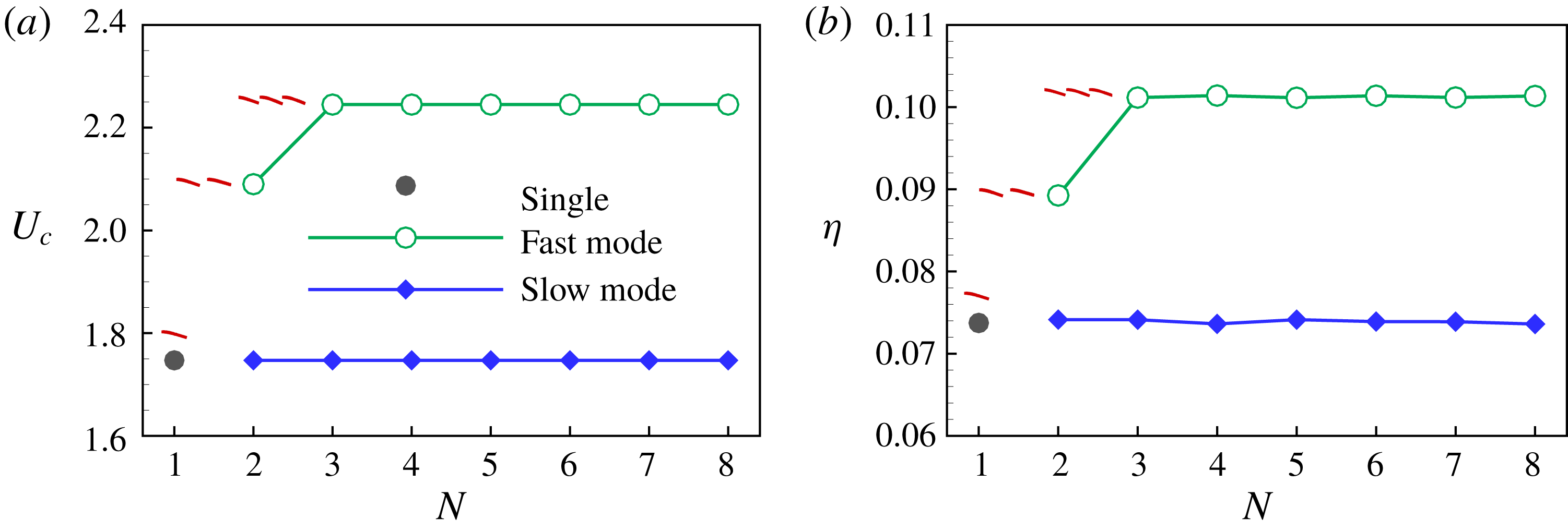
Figure 7. Schooling performance of the groups. (a) The cruising speed and (b) the swimming efficiency as a function of the group size  $N$ . Small snapshots of the leading subgroup or individual are shown in red.

Figure 7(a,b) show the cruising speed and the swimming efficiency of the group as a function of $N$ for the cases in figure 1(b,c). For the slow mode, the groups’ cruising speeds and their efficiencies are almost identical to those of the isolated swimmer. In contrast, for the fast mode, the groups have larger $U_{c}$ with higher $\unicode[STIX]{x1D702}$ compared to the isolated case. For the groups with $N>3$ , $U_{c}\approx 2.24$ and $\unicode[STIX]{x1D702}\approx 0.10$ , they are approximately 1.3 times those of the isolated plate, as shown in figure 7.

Moreover, it is interesting to see that the leading subgroup plays the role of ‘leading goose’; namely, the following subgroups or individuals would keep pace with the leading ones to achieve a uniform cruising speed, although they may have different speeds in isolated swimming. Taking case ‘C3+C2+1’ (see figure 1) as an example, we can see that if the subgroups ‘C3’, ‘C2’, and the individual ‘1’ swim independently, the cruising speeds are 2.24, 2.09 and 1.75 (see table 1), respectively. However, when swimming together as a group, they achieve a uniform cruising speed $U_{c}=2.24$ , as shown in figure 7(a). Meanwhile, the swimming efficiency of the group members ‘C2’ and ‘1’ is improved (see figure 7 b). In the fast mode, following the leading packed subgroup, the rear subgroups or individuals take advantage of the oncoming wake. These conclusions indicate the hydrodynamic force not only acts as an restoring force to maintain schooling cohesion but also provides a drafting force to rear subgroups so as to improve their schooling performance.