


1 Introduction
It is known that large-amplitude humps forming from an interfacial instability on the surface of a wall-bounded fluid film can spontaneously slide and break the symmetry of the solution. This has been observed for drops on a liquid film suspended from a ceiling (Glasner Reference Glasner2007), bubbles underneath a settling liquid droplet (Lister, Morrison & Rallison Reference Lister, Morrison and Rallison2006a ) and collars on mucus films within pulmonary capillaries (Dietze & Ruyer-Quil Reference Dietze and Ruyer-Quil2015). Lister et al. (Reference Lister, Morrison and Rallison2006a ) have conjectured that sliding results from an instability. This has prompted us to revisit the problem by investigating the stability of the symmetrical nonlinear base state (Hammond Reference Hammond1983) from which the sliding motion departs. We do this for the representative case of a liquid film suspended from a ceiling subject to the Rayleigh–Taylor instability (figure 1 a). Several new contributions have come out of our stability analysis: (i) we show that sliding results from a secondary instability of the nonlinear base state; (ii) through a frozen-time analysis, we identify a single unstable, unsymmetrical, exponentially growing eigenmode, that constitutes a concerted sliding motion of large-amplitude humps and the residual film that separates them; (iii) we explain the governing mechanism of the sliding instability, i.e. why there is a positive feedback amplifying the aforementioned eigenmode; (iv) through transient stability analysis, we show that the sliding eigenmode is most-effectively triggered by locally perturbing the very thin secondary troughs which form on the residual film; and (v) that the base state is unstable to such perturbations well before a quasi-steady state is reached but that sliding is effectively observed only within this regime.

Figure 1. Problem sketch and notations:
 $x$
,
$x$
,
 $y$
,
$y$
,
 $h$
,
$h$
,
 $D$
and
$D$
and
 $\unicode[STIX]{x1D6EC}$
have been non-dimensionalized with the average film thickness
$\unicode[STIX]{x1D6EC}$
have been non-dimensionalized with the average film thickness
 $h_{0}$
, so
$h_{0}$
, so
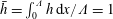 $\bar{h}=\int _{0}^{\unicode[STIX]{x1D6EC}}h\,\text{d}x/\unicode[STIX]{x1D6EC}=1$
. The film spans
$\bar{h}=\int _{0}^{\unicode[STIX]{x1D6EC}}h\,\text{d}x/\unicode[STIX]{x1D6EC}=1$
. The film spans
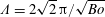
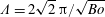 $\unicode[STIX]{x1D6EC}=2\sqrt{2}\,\unicode[STIX]{x03C0}/\sqrt{\mathit{Bo}}$
with
$\unicode[STIX]{x1D6EC}=2\sqrt{2}\,\unicode[STIX]{x03C0}/\sqrt{\mathit{Bo}}$
with
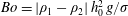 $\mathit{Bo}=|\unicode[STIX]{x1D70C}_{1}-\unicode[STIX]{x1D70C}_{2}|\,h_{0}^{2}\,g/\unicode[STIX]{x1D70E}$
, i.e. the most-amplified wavelength of the Rayleigh–Taylor instability for a passive atmosphere. A slip boundary at
$\mathit{Bo}=|\unicode[STIX]{x1D70C}_{1}-\unicode[STIX]{x1D70C}_{2}|\,h_{0}^{2}\,g/\unicode[STIX]{x1D70E}$
, i.e. the most-amplified wavelength of the Rayleigh–Taylor instability for a passive atmosphere. A slip boundary at
 $y=D$
, with
$y=D$
, with
 $1\ll D\ll \unicode[STIX]{x1D6EC}$
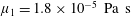
, mimics an unconfined outer phase. (a) Water film suspended from a ceiling:
$1\ll D\ll \unicode[STIX]{x1D6EC}$
, mimics an unconfined outer phase. (a) Water film suspended from a ceiling:
 $\mathit{Bo}=0.134$
(
$\mathit{Bo}=0.134$
(
 $h_{0}=1~\text{mm}$
,
$h_{0}=1~\text{mm}$
,
 $\unicode[STIX]{x1D70C}_{1}=998.2~\text{kg}~\text{m}^{-3}$
,
$\unicode[STIX]{x1D70C}_{1}=998.2~\text{kg}~\text{m}^{-3}$
,
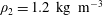 $\unicode[STIX]{x1D70C}_{2}=1.2~\text{kg}~\text{m}^{-3}$
,
$\unicode[STIX]{x1D70C}_{2}=1.2~\text{kg}~\text{m}^{-3}$
,
 $\unicode[STIX]{x1D707}_{1}=10^{-3}~\text{Pa}~\text{s}$
,
$\unicode[STIX]{x1D707}_{1}=10^{-3}~\text{Pa}~\text{s}$
,
 $\unicode[STIX]{x1D707}_{2}=1.8\times 10^{-5}~\text{Pa}~\text{s}$
,
$\unicode[STIX]{x1D707}_{2}=1.8\times 10^{-5}~\text{Pa}~\text{s}$
,
 $\unicode[STIX]{x1D70E}=0.073~\text{N}~\text{m}^{-1}$
,
$\unicode[STIX]{x1D70E}=0.073~\text{N}~\text{m}^{-1}$
,
 $D=4$
); (b) gas film underneath a liquid layer with properties according to experiments of Burton et al. (Reference Burton, Sharpe, van der Veen, Franco and Nagel2012):
$D=4$
); (b) gas film underneath a liquid layer with properties according to experiments of Burton et al. (Reference Burton, Sharpe, van der Veen, Franco and Nagel2012):
 $\mathit{Bo}=0.0016$
(
$\mathit{Bo}=0.0016$
(
 $h_{0}=100~\unicode[STIX]{x03BC}\text{m}$
,
$h_{0}=100~\unicode[STIX]{x03BC}\text{m}$
,
 $\unicode[STIX]{x1D70C}_{1}=0.47~\text{kg}~\text{m}^{-3}$
,
$\unicode[STIX]{x1D70C}_{1}=0.47~\text{kg}~\text{m}^{-3}$
,
 $\unicode[STIX]{x1D70C}_{2}=958.4~\text{kg}~\text{m}^{-3}$
,
$\unicode[STIX]{x1D70C}_{2}=958.4~\text{kg}~\text{m}^{-3}$
,
 $\unicode[STIX]{x1D707}_{1}=1.8\times 10^{-5}~\text{Pa}~\text{s}$
,
$\unicode[STIX]{x1D707}_{1}=1.8\times 10^{-5}~\text{Pa}~\text{s}$
,
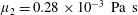 $\unicode[STIX]{x1D707}_{2}=0.28\times 10^{-3}~\text{Pa}~\text{s}$
,
$\unicode[STIX]{x1D707}_{2}=0.28\times 10^{-3}~\text{Pa}~\text{s}$
,
 $\unicode[STIX]{x1D70E}=0.059~\text{N}~\text{m}^{-1}$
,
$\unicode[STIX]{x1D70E}=0.059~\text{N}~\text{m}^{-1}$
,
 $D=10$
).
$D=10$
).
Basic features of the sliding instability are illustrated in figure 2, which depicts the key stages in the evolution of a suspended water film (the orientation of the graph is flipped vertically relative to figure 1 a). After the initial development of the Rayleigh–Taylor instability (figure 2 a–c), the thin residual film in between large drops flattens as it approaches the no-slip wall and then buckles, forming a central secondary hump out of which fluid drains symmetrically into the drops, via extremely thin secondary troughs (figure 2 d–f and supplementary movie 1 available at https://doi.org/10.1017/jfm.2018.724). This flow is maintained in the face of strong viscous stresses by capillary pressure gradients associated with curvature variations of the interface across the troughs. At this stage, the film’s evolution is quasi-steady and its symmetry is closely linked to the shapes of the two secondary troughs, which remain mutually symmetric for a very long time. Eventually, however, symmetry is lost and the film begins to slide (figure 2 g–i and supplementary movie 2). As will be shown later, the asymmetry initially appears as a flattening and thinning of one trough and simultaneous curving and thickening of the other. This creates a flow imbalance within the secondary hump, more fluid is drained through the thicker trough, which feeds back onto the shape of the film in a manner reinforcing the initial asymmetry.
From an energetic point of view, the primary instability guides the film from its initial state toward a lower-energy static equilibrium state consisting of sinusoidal drops separated by a zero-thickness film (Yiantsios & Higgins Reference Yiantsios and Higgins1989; Lister et al. Reference Lister, Rallison, King, Cummings and Jensen2006b ). To reach this state, the residual film in between drops needs to fully drain through the secondary troughs. We have found that the total drainage rate is larger when these troughs are unsymmetric, i.e. when one is thinner than the other. In the face of viscous drag, it is easier for the fluid to drain through one thick trough rather than two thin ones (figure 12). Thus, unsymmetric drainage is energetically favourable over symmetric drainage, i.e. the lower-energy droplet state can be reached faster. However, explaining the spontaneous emergence of this asymmetry and its evolution into a concerted sliding motion requires a stability analysis.
We first focus on the simple case of a single fluid phase and use a combination of numerical simulations and linear stability analyses to identify the essential ingredients necessary for sliding. This insight allows us to anticipate other, more complex, situations in which sliding should occur. At the same time, it also suggests ways to suppress sliding. We pursue both these avenues: (i) we demonstrate that all features of the sliding instability are retained in the case of a very thin gas film underneath a liquid layer (figure 1 b), assuming physical properties typically encountered underneath Leidenfrost drops (Burton et al. Reference Burton, Sharpe, van der Veen, Franco and Nagel2012) but without accounting for evaporation. Such drops are known to move autonomously even on flat surfaces (Ma, Liétor-Santos & Burton Reference Ma, Liétor-Santos and Burton2015); (ii) we show that sliding can be suppressed by thermal Marangoni stresses and we identify which ingredients of the instability mechanism this negates, explaining why sliding does not occur in the traditional Marangoni problem (Boos & Thess Reference Boos and Thess1999; Oron Reference Oron2000).

Figure 2. Evolution of the suspended water film (figure 1
a,
 $\mathit{Bo}=0.134$
) from an unstable flat surface perturbed symmetrically at the wavelength
$\mathit{Bo}=0.134$
) from an unstable flat surface perturbed symmetrically at the wavelength
 $\unicode[STIX]{x1D6EC}=2\sqrt{2}\,\unicode[STIX]{x03C0}/\sqrt{\mathit{Bo}}$
. The orientation of the graphs is flipped vertically with respect to figure 1(a). Plus signs mark the wall and the middle of the domain. Early on (a–c), growth of the Rayleigh–Taylor instability is progressive. Then, it slows under the increasing influence of the wall, causing the trough to flatten (d) and buckle (e). The resulting quasi-steady two-trough shape (f) spontaneously loses symmetry (g), causing the film to slide to the left (h,i). Two supplementary movies, movie 1 and movie 2, show these evolution stages in action.
$\unicode[STIX]{x1D6EC}=2\sqrt{2}\,\unicode[STIX]{x03C0}/\sqrt{\mathit{Bo}}$
. The orientation of the graphs is flipped vertically with respect to figure 1(a). Plus signs mark the wall and the middle of the domain. Early on (a–c), growth of the Rayleigh–Taylor instability is progressive. Then, it slows under the increasing influence of the wall, causing the trough to flatten (d) and buckle (e). The resulting quasi-steady two-trough shape (f) spontaneously loses symmetry (g), causing the film to slide to the left (h,i). Two supplementary movies, movie 1 and movie 2, show these evolution stages in action.
To set our study in the context of previous research, we discuss four works in particular. Yiantsios & Higgins (Reference Yiantsios and Higgins1989) considered a viscous fluid film underneath a heavier fluid in the limit of Stokes flow. When an asymmetric initial perturbation was applied to the flat-film base state, large differently sized humps produced by the primary Rayleigh–Taylor instability were observed to slide along the wall, whereas, when the initial perturbation was symmetrical, the film evolved toward a perfectly symmetrical quasi-steady state. Based on the results of our study, this quasi-steady state would ultimately have become unstable and slid if the simulation had been continued. We have verified this with our own calculation and this finding contradicts Yiantsios and Higgins, who believed that drops could not begin to slide from their symmetrical initial conditions.
Lister et al. (Reference Lister, Rallison, King, Cummings and Jensen2006b
) observed liquid collars sliding on an annular fluid film coating the outer surface of a cylinder of radius
 $R$
and subject to the Plateau–Rayleigh instability. A lubrication equation was obtained in the limit of a small film thickness to tube radius ratio, in which case the mathematical description collapses to that of a Rayleigh–Taylor problem. Simulations with this equation were performed on a domain representing one half of a symmetrically perturbed film of wavelength
$R$
and subject to the Plateau–Rayleigh instability. A lubrication equation was obtained in the limit of a small film thickness to tube radius ratio, in which case the mathematical description collapses to that of a Rayleigh–Taylor problem. Simulations with this equation were performed on a domain representing one half of a symmetrically perturbed film of wavelength
 $\unicode[STIX]{x1D6EC}$
. Symmetry conditions were imposed at the lateral boundaries of this domain. No sliding was observed on short domains, i.e. when the wavelength
$\unicode[STIX]{x1D6EC}$
. Symmetry conditions were imposed at the lateral boundaries of this domain. No sliding was observed on short domains, i.e. when the wavelength
 $\unicode[STIX]{x1D6EC}$
was lower or equal to twice the cutoff wavelength
$\unicode[STIX]{x1D6EC}$
was lower or equal to twice the cutoff wavelength
 $\unicode[STIX]{x1D6EC}_{c}=2\unicode[STIX]{x03C0}R$
of the primary instability. In that case, which is the one we consider here, there is a single possible final equilibrium state (Hammond Reference Hammond1983; Yiantsios & Higgins Reference Yiantsios and Higgins1989) and sliding can only occur due to a spontaneous loss of symmetry of the corresponding quasi-steady state. This was precluded in the simulations of Lister et al. (Reference Lister, Rallison, King, Cummings and Jensen2006b
) because they used symmetrical boundary conditions. On longer domains, i.e. when
$\unicode[STIX]{x1D6EC}_{c}=2\unicode[STIX]{x03C0}R$
of the primary instability. In that case, which is the one we consider here, there is a single possible final equilibrium state (Hammond Reference Hammond1983; Yiantsios & Higgins Reference Yiantsios and Higgins1989) and sliding can only occur due to a spontaneous loss of symmetry of the corresponding quasi-steady state. This was precluded in the simulations of Lister et al. (Reference Lister, Rallison, King, Cummings and Jensen2006b
) because they used symmetrical boundary conditions. On longer domains, i.e. when
 $\unicode[STIX]{x1D6EC}>2\unicode[STIX]{x1D6EC}_{c}$
, Lister et al. (Reference Lister, Rallison, King, Cummings and Jensen2006b
) did observe sliding. This resulted from an asymmetric distribution of differently sized humps emerging from the nonlinear evolution of the primary instability. These humps had the freedom to move, because, for
$\unicode[STIX]{x1D6EC}>2\unicode[STIX]{x1D6EC}_{c}$
, Lister et al. (Reference Lister, Rallison, King, Cummings and Jensen2006b
) did observe sliding. This resulted from an asymmetric distribution of differently sized humps emerging from the nonlinear evolution of the primary instability. These humps had the freedom to move, because, for
 $\unicode[STIX]{x1D6EC}>2\unicode[STIX]{x1D6EC}_{c}$
, there exist an infinite number of possible final states, which differ in terms of the number, volume and separation of sinusoidal equilibrium humps (Yiantsios & Higgins Reference Yiantsios and Higgins1989).
$\unicode[STIX]{x1D6EC}>2\unicode[STIX]{x1D6EC}_{c}$
, there exist an infinite number of possible final states, which differ in terms of the number, volume and separation of sinusoidal equilibrium humps (Yiantsios & Higgins Reference Yiantsios and Higgins1989).
For very long domains, Lister et al. (Reference Lister, Rallison, King, Cummings and Jensen2006b ) found that a sliding hump can repeatedly bounce back and forth between two neighbours pinned to the symmetric domain boundaries. As the hump slides, it peels off the thin film lying in front of it and re-deposits a thinner film at its trailing edge. It was shown that the film thickness there obeys the Landau–Levich equation (Landau & Levich Reference Landau and Levich1942), where only variations of longitudinal curvature and radial viscous diffusion intervene.
In a companion paper, Lister et al. (Reference Lister, Morrison and Rallison2006a ) applied their lubrication equation to describe the drainage of a fluid film underneath a droplet settling toward a wall. In particular, the authors report one simulation where a bubble forming underneath the droplet spontaneously slides, and they deduce that this must result from an instability.
The fourth study is that of Glasner (Reference Glasner2007), who used a lubrication equation to simulate two-dimensional drops sliding on a liquid film suspended from a permeable ceiling that continuously supplies additional fluid. In the case of multiple drops, collisions occur and the author showed that these are always repulsive, confirming the observations of Lister et al. (Reference Lister, Rallison, King, Cummings and Jensen2006b ). Most of Glasner’s simulations were started from a nonlinear asymmetrical initial condition which, according to the author, guaranteed the migration of droplets. However, in one simulation, the initial condition consisted of a weak (unspecified) asymmetrical perturbation of the uniform film. Interestingly, although slight asymmetry was present at the start, droplets slid only after a quasi-steady seemingly symmetrical state had been reached (the above-mentioned simulation of Lister et al. (Reference Lister, Morrison and Rallison2006a ) behaved the same way). This raises the question whether the transient evolution toward a quasi-steady state is stable with respect to sliding. We answer this question in the present manuscript by applying transient stability analysis (Schmid Reference Schmid2007; Balestra, Brun & Gallaire Reference Balestra, Brun and Gallaire2016).
Glasner (Reference Glasner2007) also introduced a reduced model to describe the dynamics of sliding drops. This model consists of a drop in static equilibrium situated between two thin films of uniform but different thickness, which are connected to the drop by so-called internal layers. Based on a thought experiment, the author demonstrated that it is energetically favourable for the drop to slide toward the thicker rather than toward the thinner film. However, it remained to be shown whether a sliding drop is energetically favourable over a purely symmetrical non-sliding evolution. Our current manuscript provides this missing information by showing that drops slide as the result of a secondary instability, drainage toward their final equilibrium state occurring quicker than in a symmetric evolution.
We point out that observing sliding in a particular numerical experiment is not the same as performing a linear stability analysis of the symmetrical base state from which the sliding motion departs. A stability analysis allows the identification of the most unstable among all possible perturbations. This perturbation maximizes destabilizing versus stabilizing contributions and thus allows the identification of the instability mechanism. Our frozen-time analysis has uncovered a single exponentially growing sliding eigenmode and our transient analysis has shown that this mode is most-effectively triggered by locally perturbing the secondary troughs.
We study the sliding instability with a long-wave model obtained in the framework of the weighted residual integral boundary layer (WRIBL) method (Ruyer-Quil & Manneville Reference Ruyer-Quil and Manneville2002). We use this model to simulate the evolution of an initially flat-film surface subjected to an unstable symmetrical perturbation of wavelength
 $\unicode[STIX]{x1D6EC}$
. We distinguish two types of simulations. The first type represents the entire wavelength
$\unicode[STIX]{x1D6EC}$
. We distinguish two types of simulations. The first type represents the entire wavelength
 $\unicode[STIX]{x1D6EC}$
and a periodicity condition is imposed at the lateral boundaries of the domain. The film is thus allowed to slide sideways as a whole, shifting its centre of gravity, but nothing in the initial arrangement orients toward such an event. Sliding, if it occurs, is triggered by numerical noise as the result of an instability. Such simulations allow us to identify when symmetry is lost. The second type of simulation represents
$\unicode[STIX]{x1D6EC}$
and a periodicity condition is imposed at the lateral boundaries of the domain. The film is thus allowed to slide sideways as a whole, shifting its centre of gravity, but nothing in the initial arrangement orients toward such an event. Sliding, if it occurs, is triggered by numerical noise as the result of an instability. Such simulations allow us to identify when symmetry is lost. The second type of simulation represents
 $\unicode[STIX]{x1D6EC}/2$
and symmetry conditions are imposed at the domain boundaries. This allows us to produce a perfectly symmetrical base state, upon which we then perform a stability analysis (after having mirrored the solution onto the full wavelength
$\unicode[STIX]{x1D6EC}/2$
and symmetry conditions are imposed at the domain boundaries. This allows us to produce a perfectly symmetrical base state, upon which we then perform a stability analysis (after having mirrored the solution onto the full wavelength
 $\unicode[STIX]{x1D6EC}$
).
$\unicode[STIX]{x1D6EC}$
).
Our WRIBL model in its full form accounts for inertia, longitudinal viscous diffusion, and the interaction with an outer phase. By comparing results in the limit of creeping flow with the full-model prediction, we show that inertia, although affecting the early dynamics of the film, does not trigger sliding before a quasi-steady state is reached and does not alter this state. The dominant physics of the sliding instability can thus be treated in the framework of lubrication theory and we use an appropriate simplified version of our model for most of the remaining manuscript. We then revert back to the full model to treat the related problem of a gas film underneath a much more viscous liquid layer (figure 1 b), which we consider in § 8. Throughout the manuscript, full model will be used to refer to the full form of the WRIBL model, notwithstanding that this still constitutes an approximation of the Navier–Stokes equations.
All our calculations concern films of either liquid water (figure 1
a) or water vapour (figure 1
b). In both cases, the observed minimal film thickness upon sliding is at least two orders of magnitude greater than the range of long-range van der Waals forces, which is of the order of
 ${\approx}10$
nm (Bonn Reference Bonn2009; Israelachvili Reference Israelachvili2011). Thus, sliding is expected to occur before spinodal film rupture and the sliding instability ought to be experimentally observable. Parameters for the studied cases, which are specified in the caption of figure 1 and will remain unchanged throughout, are chosen accordingly.
${\approx}10$
nm (Bonn Reference Bonn2009; Israelachvili Reference Israelachvili2011). Thus, sliding is expected to occur before spinodal film rupture and the sliding instability ought to be experimentally observable. Parameters for the studied cases, which are specified in the caption of figure 1 and will remain unchanged throughout, are chosen accordingly.
Our manuscript is structured as follows. In § 2, we present the employed mathematical models and introduce our scaling. We then focus on the problem of a water film suspended from a ceiling (figure 1 a). In § 3, we describe the kinematics of the film evolution, from the linear stage of the primary instability, through the nonlinear symmetrical quasi-steady state, up to the onset of sliding. In § 4, we discuss the draining mechanisms leading up to the quasi-steady state. In § 5, we perform a frozen-time linear stability analysis of this quasi-steady state and, in § 6, we deconstruct the mechanism of the sliding instability. In § 7, we investigate the stability of the evolving base state using transient stability analysis, and determine the sensitivity of the sliding onset to noise. In § 8, we show that the sliding instability also occurs in a gas film underneath a liquid (figure 1 b), assuming physical properties typically encountered underneath Leidenfrost drops (Burton et al. Reference Burton, Sharpe, van der Veen, Franco and Nagel2012). Conversely, we demonstrate in § 9 that adding thermal Marangoni stresses can suppress the sliding instability mechanism. Conclusions are drawn in § 10.
2 Mathematical models
We consider the two configurations in figures 1(a) and 1(b), where both phases consist of Newtonian fluids with constant density
 $\unicode[STIX]{x1D70C}_{i}$
and viscosity
$\unicode[STIX]{x1D70C}_{i}$
and viscosity
 $\unicode[STIX]{x1D707}_{i}$
(the subscript
$\unicode[STIX]{x1D707}_{i}$
(the subscript
 $i=1,2$
differentiates between the two phases), and where
$i=1,2$
differentiates between the two phases), and where
 $g$
designates gravitational acceleration. The surface tension
$g$
designates gravitational acceleration. The surface tension
 $\unicode[STIX]{x1D70E}$
will be assumed constant except in § 9, where we will study the additional effect of thermal Marangoni stresses. We assume that the (dimensionless) film thickness
$\unicode[STIX]{x1D70E}$
will be assumed constant except in § 9, where we will study the additional effect of thermal Marangoni stresses. We assume that the (dimensionless) film thickness
 $h$
is small compared to the (dimensionless) wavelength
$h$
is small compared to the (dimensionless) wavelength
 $\unicode[STIX]{x1D6EC}$
and use the weighted residual integral boundary layer (WRIBL) model of Dietze & Ruyer-Quil (Reference Dietze and Ruyer-Quil2013), which accounts for inertia, longitudinal viscous diffusion and inter-phase coupling. In dimensionless form, this reads:
$\unicode[STIX]{x1D6EC}$
and use the weighted residual integral boundary layer (WRIBL) model of Dietze & Ruyer-Quil (Reference Dietze and Ruyer-Quil2013), which accounts for inertia, longitudinal viscous diffusion and inter-phase coupling. In dimensionless form, this reads:
 $$\begin{eqnarray}\unicode[STIX]{x2202}_{t}h=-\unicode[STIX]{x2202}_{x}q_{1},\quad q_{tot}(t)=q_{1}+q_{2},\end{eqnarray}$$
 $$\begin{eqnarray}\displaystyle \mathit{Re}\{S_{i}\unicode[STIX]{x2202}_{t}q_{i}+F_{ij}q_{i}\unicode[STIX]{x2202}_{x}q_{j}+G_{ij}q_{i}q_{j}\unicode[STIX]{x2202}_{x}h\} & = & \displaystyle \pm (1-\unicode[STIX]{x1D6F1}_{\unicode[STIX]{x1D70C}})\unicode[STIX]{x2202}_{x}h-\mathit{Bo}^{-1}\unicode[STIX]{x2202}_{x}[\unicode[STIX]{x1D705}]+(C_{j1}-\unicode[STIX]{x1D6F1}_{\unicode[STIX]{x1D707}}C_{j2})q_{j}\nonumber\\ \displaystyle & & \displaystyle +\,J_{j}\,q_{j}(\unicode[STIX]{x2202}_{x}h)^{2}+K_{j}\unicode[STIX]{x2202}_{x}q_{j}\unicode[STIX]{x2202}_{x}h+L_{j}q_{j}\unicode[STIX]{x2202}_{xx}h+M_{j}\unicode[STIX]{x2202}_{xx}q_{j},\nonumber\\ \displaystyle & & \displaystyle\end{eqnarray}$$
 $i$
and
$i$
and
 $j$
are to be permuted through the phase indices 1 and 2 using Einstein summation. In (2.1),
$j$
are to be permuted through the phase indices 1 and 2 using Einstein summation. In (2.1),
 $h$
designates the film thickness,
$h$
designates the film thickness,
 $q_{i}$
the phase-specific flow rate per unit width and
$q_{i}$
the phase-specific flow rate per unit width and
 $\unicode[STIX]{x1D705}=\unicode[STIX]{x2202}_{xx}h$
the interfacial curvature (at second order in the long-wave expansion). Following Yiantsios & Higgins (Reference Yiantsios and Higgins1989), we have used for non-dimensionalization the length scale
$\unicode[STIX]{x1D705}=\unicode[STIX]{x2202}_{xx}h$
the interfacial curvature (at second order in the long-wave expansion). Following Yiantsios & Higgins (Reference Yiantsios and Higgins1989), we have used for non-dimensionalization the length scale
 ${\mathcal{L}}=h_{0}$
, corresponding to the average film thickness, the velocity scale
${\mathcal{L}}=h_{0}$
, corresponding to the average film thickness, the velocity scale
 ${\mathcal{U}}=|\unicode[STIX]{x0394}\unicode[STIX]{x1D70C}|gh_{0}^{2}/\unicode[STIX]{x1D707}_{1}$
with
${\mathcal{U}}=|\unicode[STIX]{x0394}\unicode[STIX]{x1D70C}|gh_{0}^{2}/\unicode[STIX]{x1D707}_{1}$
with
 $\unicode[STIX]{x0394}\unicode[STIX]{x1D70C}=\unicode[STIX]{x1D70C}_{1}-\unicode[STIX]{x1D70C}_{2}$
, obtained by balancing viscous drag and gravity, and the time scale
$\unicode[STIX]{x0394}\unicode[STIX]{x1D70C}=\unicode[STIX]{x1D70C}_{1}-\unicode[STIX]{x1D70C}_{2}$
, obtained by balancing viscous drag and gravity, and the time scale
 ${\mathcal{T}}={\mathcal{L}}/{\mathcal{U}}=\unicode[STIX]{x1D707}_{1}/|\unicode[STIX]{x0394}\unicode[STIX]{x1D70C}|/g/h_{0}$
. This choice yields the Reynolds number
${\mathcal{T}}={\mathcal{L}}/{\mathcal{U}}=\unicode[STIX]{x1D707}_{1}/|\unicode[STIX]{x0394}\unicode[STIX]{x1D70C}|/g/h_{0}$
. This choice yields the Reynolds number
 $\mathit{Re}={\mathcal{U}}h_{0}|\unicode[STIX]{x0394}\unicode[STIX]{x1D70C}|/\unicode[STIX]{x1D707}_{1}$
and the Bond number
$\mathit{Re}={\mathcal{U}}h_{0}|\unicode[STIX]{x0394}\unicode[STIX]{x1D70C}|/\unicode[STIX]{x1D707}_{1}$
and the Bond number
 $\mathit{Bo}=|\unicode[STIX]{x0394}\unicode[STIX]{x1D70C}|gh_{0}^{2}/\unicode[STIX]{x1D70E}$
, which are completed by the density and viscosity ratios
$\mathit{Bo}=|\unicode[STIX]{x0394}\unicode[STIX]{x1D70C}|gh_{0}^{2}/\unicode[STIX]{x1D70E}$
, which are completed by the density and viscosity ratios
 $\unicode[STIX]{x1D6F1}_{\unicode[STIX]{x1D70C}}=\unicode[STIX]{x1D70C}_{2}/\unicode[STIX]{x1D70C}_{1}$
and
$\unicode[STIX]{x1D6F1}_{\unicode[STIX]{x1D70C}}=\unicode[STIX]{x1D70C}_{2}/\unicode[STIX]{x1D70C}_{1}$
and
 $\unicode[STIX]{x1D6F1}_{\unicode[STIX]{x1D707}}=\unicode[STIX]{x1D707}_{2}/\unicode[STIX]{x1D707}_{1}$
. At places, we will also relate the dimensionless horizontal coordinate
$\unicode[STIX]{x1D6F1}_{\unicode[STIX]{x1D707}}=\unicode[STIX]{x1D707}_{2}/\unicode[STIX]{x1D707}_{1}$
. At places, we will also relate the dimensionless horizontal coordinate
 $x$
to the dimensionless wavelength
$x$
to the dimensionless wavelength
 $\unicode[STIX]{x1D6EC}$
.
$\unicode[STIX]{x1D6EC}$
. In (2.1c
), the sign of the gravity term (first term on the right-hand side) is positive for the suspended film (figure 1
a) and negative for the gas film (figure 1
b). The coefficients
 $F_{ij}$
,
$F_{ij}$
,
 $G_{ij}$
,
$G_{ij}$
,
 $C_{ij}$
,
$C_{ij}$
,
 $S_{j}$
,
$S_{j}$
,
 $J_{j}$
,
$J_{j}$
,
 $K_{j}$
and
$K_{j}$
and
 $M_{j}$
are known functions of
$M_{j}$
are known functions of
 $h$
and the domain height
$h$
and the domain height
 $D$
. Our coefficients are slightly different than in Dietze & Ruyer-Quil (Reference Dietze and Ruyer-Quil2013), as we impose a slip boundary at
$D$
. Our coefficients are slightly different than in Dietze & Ruyer-Quil (Reference Dietze and Ruyer-Quil2013), as we impose a slip boundary at
 $y=D$
(
$y=D$
(
 $\unicode[STIX]{x2202}_{y}u|_{D}=v|_{D}=0$
) instead of a wall (the coefficient definitions have been provided in a Mathematica® file in the supplementary material). The slip boundary is sufficiently far to prevent influencing the large humps produced by the primary instability, i.e.
$\unicode[STIX]{x2202}_{y}u|_{D}=v|_{D}=0$
) instead of a wall (the coefficient definitions have been provided in a Mathematica® file in the supplementary material). The slip boundary is sufficiently far to prevent influencing the large humps produced by the primary instability, i.e.
 $D\gg 1$
, and sufficiently close to satisfy the long-wave approximation in both layers, i.e.
$D\gg 1$
, and sufficiently close to satisfy the long-wave approximation in both layers, i.e.
 $D\ll \unicode[STIX]{x1D6EC}$
. We have verified for both the suspended film (figure 1
a,
$D\ll \unicode[STIX]{x1D6EC}$
. We have verified for both the suspended film (figure 1
a,
 $D=4=0.16\unicode[STIX]{x1D6EC}$
) and the gas film (figure 1
b,
$D=4=0.16\unicode[STIX]{x1D6EC}$
) and the gas film (figure 1
b,
 $D=10=0.04\unicode[STIX]{x1D6EC}$
) that the quasi-steady state reached prior to sliding is virtually insensitive to
$D=10=0.04\unicode[STIX]{x1D6EC}$
) that the quasi-steady state reached prior to sliding is virtually insensitive to
 $D$
. In this sense, our simulations mimic an unconfined outer phase.
$D$
. In this sense, our simulations mimic an unconfined outer phase.
We solve (2.1) numerically, using second-order central differences for spatial and the Crank–Nicolson method for time discretization, and linearizing nonlinear terms around the old time step. In terms of boundary conditions, we distinguish two cases: (i) periodic simulations on a domain of length
 $\unicode[STIX]{x1D6EC}$
, where
$\unicode[STIX]{x1D6EC}$
, where
 $\unicode[STIX]{x2202}_{x^{i}}h|_{x=0}=\unicode[STIX]{x2202}_{x^{i}}h|_{x=\unicode[STIX]{x1D6EC}}$
,
$\unicode[STIX]{x2202}_{x^{i}}h|_{x=0}=\unicode[STIX]{x2202}_{x^{i}}h|_{x=\unicode[STIX]{x1D6EC}}$
,
 $\unicode[STIX]{x2202}_{x^{i}}q|_{x=0}=\unicode[STIX]{x2202}_{x^{i}}q|_{x=\unicode[STIX]{x1D6EC}}$
and the film is free to slide, and (ii) symmetric simulations on a domain of length
$\unicode[STIX]{x2202}_{x^{i}}q|_{x=0}=\unicode[STIX]{x2202}_{x^{i}}q|_{x=\unicode[STIX]{x1D6EC}}$
and the film is free to slide, and (ii) symmetric simulations on a domain of length
 $\unicode[STIX]{x1D6EC}/2$
, where
$\unicode[STIX]{x1D6EC}/2$
, where
 $\unicode[STIX]{x2202}_{x}h=\unicode[STIX]{x2202}_{xxx}h=0$
(implying
$\unicode[STIX]{x2202}_{x}h=\unicode[STIX]{x2202}_{xxx}h=0$
(implying
 $q=0$
) at
$q=0$
) at
 $x=0$
and
$x=0$
and
 $\unicode[STIX]{x1D6EC}/2$
, in order to capture the non-sliding quasi-steady solution. The dimensionless wavelength
$\unicode[STIX]{x1D6EC}/2$
, in order to capture the non-sliding quasi-steady solution. The dimensionless wavelength
 $\unicode[STIX]{x1D6EC}$
is set to the most-amplified wavelength of the Rayleigh–Taylor instability for a passive outer phase
$\unicode[STIX]{x1D6EC}$
is set to the most-amplified wavelength of the Rayleigh–Taylor instability for a passive outer phase
 $\unicode[STIX]{x1D6EC}=\sqrt{2}\unicode[STIX]{x1D6EC}_{c}$
, where
$\unicode[STIX]{x1D6EC}=\sqrt{2}\unicode[STIX]{x1D6EC}_{c}$
, where
 $\unicode[STIX]{x1D6EC}_{c}=2\unicode[STIX]{x03C0}/\sqrt{\mathit{Bo}}$
is the corresponding cutoff wavelength. This quantity is convenient because it is known in closed form and, for all our simulations, it differs by less than 0.5 per cent from the actual most-amplified wavelength (i.e. for an active outer phase). We will loosely refer to
$\unicode[STIX]{x1D6EC}_{c}=2\unicode[STIX]{x03C0}/\sqrt{\mathit{Bo}}$
is the corresponding cutoff wavelength. This quantity is convenient because it is known in closed form and, for all our simulations, it differs by less than 0.5 per cent from the actual most-amplified wavelength (i.e. for an active outer phase). We will loosely refer to
 $\sqrt{2}\unicode[STIX]{x1D6EC}_{c}$
as the most-amplified wavelength of the Rayleigh–Taylor instability.
$\sqrt{2}\unicode[STIX]{x1D6EC}_{c}$
as the most-amplified wavelength of the Rayleigh–Taylor instability.
For the suspended water film, which we mainly focus on, we have used the full model (2.1) as a reference to identify those ingredients that are sufficient for the sliding instability, i.e. gravity, surface tension and cross-wise (
 $y$
-direction) viscous diffusion. Retaining only these ingredients in (2.1), we obtain the following simplified model:
$y$
-direction) viscous diffusion. Retaining only these ingredients in (2.1), we obtain the following simplified model:
 $$\begin{eqnarray}\displaystyle & \displaystyle \unicode[STIX]{x2202}_{t}h=-\unicode[STIX]{x2202}_{x}q, & \displaystyle\end{eqnarray}$$
 $$\begin{eqnarray}\displaystyle & \displaystyle q=\frac{1}{3}\left[h^{3}\unicode[STIX]{x2202}_{x}h+\frac{1}{\mathit{Bo}}h^{3}\unicode[STIX]{x2202}_{xxx}h\right], & \displaystyle\end{eqnarray}$$
 $\unicode[STIX]{x1D6F1}_{\unicode[STIX]{x1D70C}}=\unicode[STIX]{x1D6F1}_{\unicode[STIX]{x1D707}}=0$
) and thus the phase index has been dropped. The Bond number reduces to
$\unicode[STIX]{x1D6F1}_{\unicode[STIX]{x1D70C}}=\unicode[STIX]{x1D6F1}_{\unicode[STIX]{x1D707}}=0$
) and thus the phase index has been dropped. The Bond number reduces to
 $\mathit{Bo}=\unicode[STIX]{x1D70C}_{1}gh_{0}^{2}/\unicode[STIX]{x1D70E}$
and remains the sole dimensionless group. We will use (2.2) for our stability analysis and most of the discussions in §§ 3–7. We point out that it is the same as the lubrication equation in Lister et al. (Reference Lister, Rallison, King, Cummings and Jensen2006b
).
$\mathit{Bo}=\unicode[STIX]{x1D70C}_{1}gh_{0}^{2}/\unicode[STIX]{x1D70E}$
and remains the sole dimensionless group. We will use (2.2) for our stability analysis and most of the discussions in §§ 3–7. We point out that it is the same as the lubrication equation in Lister et al. (Reference Lister, Rallison, King, Cummings and Jensen2006b
). In § 9, we will study the effect of additional thermal Marangoni stresses due to heating the suspended film from the bounding wall, assuming
 $\unicode[STIX]{x2202}_{T}\unicode[STIX]{x1D70E}<0$
. To account for this, equation (2.2b
) needs to be extended:
$\unicode[STIX]{x2202}_{T}\unicode[STIX]{x1D70E}<0$
. To account for this, equation (2.2b
) needs to be extended:
 $$\begin{eqnarray}q=\frac{1}{3}\left[h^{3}\unicode[STIX]{x2202}_{x}h+\frac{1}{\mathit{Bo}}h^{3}\unicode[STIX]{x2202}_{xxx}h\right]+\frac{1}{2}\frac{\mathit{Ma}}{\mathit{Bo}}h^{2}\unicode[STIX]{x2202}_{x}\unicode[STIX]{x1D703}|_{h},\end{eqnarray}$$
where
 $\mathit{Ma}=\unicode[STIX]{x2202}_{T}\unicode[STIX]{x1D70E}(T_{w}-T_{\infty })/\unicode[STIX]{x1D70E}$
designates a modified Marangoni number,
$\mathit{Ma}=\unicode[STIX]{x2202}_{T}\unicode[STIX]{x1D70E}(T_{w}-T_{\infty })/\unicode[STIX]{x1D70E}$
designates a modified Marangoni number,
 $\unicode[STIX]{x1D703}|_{h}=(T|_{h}-T_{w})/(T_{w}-T_{\infty })=-\mathit{Bi}\,h/(1+\mathit{Bi}\,h)$
the dimensionless film surface temperature,
$\unicode[STIX]{x1D703}|_{h}=(T|_{h}-T_{w})/(T_{w}-T_{\infty })=-\mathit{Bi}\,h/(1+\mathit{Bi}\,h)$
the dimensionless film surface temperature,
 $\mathit{Bi}=\mathscr{H}h_{0}/k_{1}$
the Biot number and
$\mathit{Bi}=\mathscr{H}h_{0}/k_{1}$
the Biot number and
 $T_{w}$
and
$T_{w}$
and
 $T_{\infty }$
the wall and ambient temperature. The Biot number contains the interfacial heat transfer coefficient
$T_{\infty }$
the wall and ambient temperature. The Biot number contains the interfacial heat transfer coefficient
 $\mathscr{H}$
and the thermal conductivity
$\mathscr{H}$
and the thermal conductivity
 $k_{1}$
. We point out that (2.3) was previously used in Alexeev & Oron (Reference Alexeev and Oron2007), where the film was cooled from the wall, and thus Marangoni stresses were stabilizing (
$k_{1}$
. We point out that (2.3) was previously used in Alexeev & Oron (Reference Alexeev and Oron2007), where the film was cooled from the wall, and thus Marangoni stresses were stabilizing (
 $\mathit{Ma}>0$
) in terms of the primary instability, as opposed to our case (we will set
$\mathit{Ma}>0$
) in terms of the primary instability, as opposed to our case (we will set
 $\mathit{Ma}=-0.2$
).
$\mathit{Ma}=-0.2$
).
In § 8, we will show that a very thin gas film underneath a (much more viscous) liquid layer is also prone to the sliding instability. For this configuration, we will use the full model (2.1) in order to account for viscous coupling with the outer phase.
All our simulations were started from a symmetric initial condition:
 $$\begin{eqnarray}h|_{t=0}=1+\unicode[STIX]{x1D700}\cos (2\unicode[STIX]{x03C0}x/\unicode[STIX]{x1D6EC}),\end{eqnarray}$$
with a very small relative perturbation amplitude
 $\unicode[STIX]{x1D700}=0.0009$
. When using the full model (2.1), the initial flow rate
$\unicode[STIX]{x1D700}=0.0009$
. When using the full model (2.1), the initial flow rate
 $q|_{t=0}$
was computed from the inertialess limit (2.2b
) using (2.4). Our initial condition ensures that sliding, if it occurs, does so spontaneously.
$q|_{t=0}$
was computed from the inertialess limit (2.2b
) using (2.4). Our initial condition ensures that sliding, if it occurs, does so spontaneously.
3 Kinematics of the sliding instability
For the time being, we focus on the configuration of a suspended water film of average thickness
 $h_{0}=1~\text{mm}$
and
$h_{0}=1~\text{mm}$
and
 $\mathit{Bo}=0.134$
which is surrounded by air, as illustrated in figure 1(a) (see caption for other properties). We have simulated the evolution of this film with the full (2.1) and simplified (2.2) models, starting from the fully symmetrical initial condition (2.4) (perturbation amplitude
$\mathit{Bo}=0.134$
which is surrounded by air, as illustrated in figure 1(a) (see caption for other properties). We have simulated the evolution of this film with the full (2.1) and simplified (2.2) models, starting from the fully symmetrical initial condition (2.4) (perturbation amplitude
 $\unicode[STIX]{x1D700}=0.0009$
), using periodic boundary conditions on a domain spanning the wavelength
$\unicode[STIX]{x1D700}=0.0009$
), using periodic boundary conditions on a domain spanning the wavelength
 $\unicode[STIX]{x1D6EC}=2\sqrt{2}\unicode[STIX]{x03C0}/\sqrt{\mathit{Bo}}=24.2$
and discretized with 1001 grid points. Figure 3 shows how the film evolves from the symmetrical initial state to an asymmetrical sliding state through four characteristic stages, which are also discernible in figure 2. In contrast to figure 1(a), gravity points upward in figures 2 and 3.
$\unicode[STIX]{x1D6EC}=2\sqrt{2}\unicode[STIX]{x03C0}/\sqrt{\mathit{Bo}}=24.2$
and discretized with 1001 grid points. Figure 3 shows how the film evolves from the symmetrical initial state to an asymmetrical sliding state through four characteristic stages, which are also discernible in figure 2. In contrast to figure 1(a), gravity points upward in figures 2 and 3.

Figure 3. Kinematics of the sliding sequence for the suspended water film (see figure 1
a):
 $h_{0}=1~\text{mm}$
,
$h_{0}=1~\text{mm}$
,
 $\mathit{Bo}=0.134$
,
$\mathit{Bo}=0.134$
,
 $\unicode[STIX]{x1D6EC}=24.2$
. In (a,b), dashed lines correspond to the full model (2.1), solid lines to (2.2), and the red solid line in (b) to a simulation of the full Navier–Stokes equations (discussed at the end of § 3). Symbols refer to characteristic stages in (c–f), where profiles evolve from dashed to dot–dashed lines. The horizontal coordinate
$\unicode[STIX]{x1D6EC}=24.2$
. In (a,b), dashed lines correspond to the full model (2.1), solid lines to (2.2), and the red solid line in (b) to a simulation of the full Navier–Stokes equations (discussed at the end of § 3). Symbols refer to characteristic stages in (c–f), where profiles evolve from dashed to dot–dashed lines. The horizontal coordinate
 $x$
has been related to the (dimensionless) domain length
$x$
has been related to the (dimensionless) domain length
 $\unicode[STIX]{x1D6EC}$
. (a) Time trace of the trough position (left trough after buckling); (b) film thickness at trough position corresponding to (a); (c) surface profiles during first stage: progressive growth; (d) flattening and buckling of the film surface; (e) quasi-steady two-trough shape (see also supplementary movie 1); (f) loss of symmetry and sliding (see also supplementary movie 2).
$\unicode[STIX]{x1D6EC}$
. (a) Time trace of the trough position (left trough after buckling); (b) film thickness at trough position corresponding to (a); (c) surface profiles during first stage: progressive growth; (d) flattening and buckling of the film surface; (e) quasi-steady two-trough shape (see also supplementary movie 1); (f) loss of symmetry and sliding (see also supplementary movie 2).
Figures 3(a) and 3(b) represent time traces of the position
 $x_{min}$
and thickness
$x_{min}$
and thickness
 $h_{min}$
of the film surface minimum. Different symbols refer to different evolution stages, which are illustrated through surface profiles in figures 3(c)–3(f). Data were obtained with the inertialess model (2.2), except for the dashed lines in figures 3(a) and 3(b), which correspond to the full model (2.1), and the red line in figure 3(b), which was obtained from a simulation of the full Navier–Stokes equations (detailed at the end of § 3). For convenience, we have normalized
$h_{min}$
of the film surface minimum. Different symbols refer to different evolution stages, which are illustrated through surface profiles in figures 3(c)–3(f). Data were obtained with the inertialess model (2.2), except for the dashed lines in figures 3(a) and 3(b), which correspond to the full model (2.1), and the red line in figure 3(b), which was obtained from a simulation of the full Navier–Stokes equations (detailed at the end of § 3). For convenience, we have normalized
 $x$
with the domain length
$x$
with the domain length
 $\unicode[STIX]{x1D6EC}$
. The large values of
$\unicode[STIX]{x1D6EC}$
. The large values of
 $t$
in figures 3(a) and 3(b) occur because sliding sets in very late in terms of the typical time scales of viscous capillary–gravity flows (Yiantsios & Higgins Reference Yiantsios and Higgins1989; Lister et al.
Reference Lister, Rallison, King, Cummings and Jensen2006b
; Glasner Reference Glasner2007).
$t$
in figures 3(a) and 3(b) occur because sliding sets in very late in terms of the typical time scales of viscous capillary–gravity flows (Yiantsios & Higgins Reference Yiantsios and Higgins1989; Lister et al.
Reference Lister, Rallison, King, Cummings and Jensen2006b
; Glasner Reference Glasner2007).
The first three evolution stages in figure 3 have been discussed in detail by Yiantsios & Higgins (Reference Yiantsios and Higgins1989) and so we recap them only briefly. In the first stage (crosses in figures 3 a and 3 b), growth of the surface perturbation is progressive and the corresponding spatial profiles (figure 3 c) exhibit a single trough that increasingly thins while remaining in the middle of the domain. During the second stage (filled circles in figures 3 a and 3 b), the film surface around the trough flattens and then buckles upon further approaching the wall, forming two secondary troughs enclosing a secondary hump in the middle (figure 3 d, where the range of the abscissa has been reduced). In figures 3(a) and 3(b), it is the left secondary trough that is tracked from the buckling event onwards. This secondary trough (and its twin on the other side) moves outward and increasingly thins. At the same time, the secondary hump in the middle grows more pronounced. This evolution continues for some time but increasingly slows down, until the film reaches a quasi-steady state (diamonds in figures 3 a and 3 b), constituting the third evolution stage. Corresponding surface profiles in figure 3(e) change only very slightly over a considerable time interval. In particular, the locations of the secondary troughs remain virtually fixed. The supplementary movie 1 shows the first three evolution stages in action (the ordinate has been scaled logarithmically to highlight the secondary troughs).
In the fourth evolution stage (open circles in figures 3
a and 3
b), the quasi-steady buckled-film surface spontaneously loses its symmetry, causing the entire film to slide to the left (figure 3
f). The supplementary movie 2 shows these events in action (the ordinate has again been scaled logarithmically). The speed of the sliding motion, based on the displacement of the right trough in figure 3(f), is roughly
 $c=1.2\times 10^{-4}$
(corresponding to a dimensional value of
$c=1.2\times 10^{-4}$
(corresponding to a dimensional value of
 $1.2~\text{mm}~\text{s}^{-1}$
).
$1.2~\text{mm}~\text{s}^{-1}$
).
We now focus on the loss of symmetry with the help of figure 4 by comparing our periodic simulation (dashed and dot–dot–dashed lines in figures 4
a–4
c) with a symmetric simulation on a domain spanning
 $\unicode[STIX]{x1D6EC}/2$
(solid lines in figures 4
a–4
c). Although the symmetric simulation represents only one of the secondary troughs, we have produced the other by mirroring the simulation data to the other side. Comparing the two solutions in figure 4(a), we conclude that symmetry is lost at
$\unicode[STIX]{x1D6EC}/2$
(solid lines in figures 4
a–4
c). Although the symmetric simulation represents only one of the secondary troughs, we have produced the other by mirroring the simulation data to the other side. Comparing the two solutions in figure 4(a), we conclude that symmetry is lost at
 $t\approx 7\times 10^{4}$
, when the periodic simulation departs from the symmetric one in that both the left and right secondary troughs move to the left. At the same time, the film thickness at the left secondary trough starts to decrease, while it increases at the right trough (figure 4
b). During the leftward migration of the secondary troughs, the film is peeled off on their right and deposited on their left, in accordance with the motion described by Lister et al. (Reference Lister, Rallison, King, Cummings and Jensen2006b
). This is comparable to a track vehicle putting down its chains while moving forward.
$t\approx 7\times 10^{4}$
, when the periodic simulation departs from the symmetric one in that both the left and right secondary troughs move to the left. At the same time, the film thickness at the left secondary trough starts to decrease, while it increases at the right trough (figure 4
b). During the leftward migration of the secondary troughs, the film is peeled off on their right and deposited on their left, in accordance with the motion described by Lister et al. (Reference Lister, Rallison, King, Cummings and Jensen2006b
). This is comparable to a track vehicle putting down its chains while moving forward.
At the left trough, deposition occurs faster than peeling and thus the trough becomes increasingly flat, whereas the opposite occurs at the right trough, which becomes increasingly curved. Quantitative evidence of this is shown in figure 4(c), which plots time traces of the surface curvature
 $\unicode[STIX]{x2202}_{xx}h$
at the two troughs. Comparing the periodic with the symmetric data after the film surface has buckled (unshaded region), shows that, at the onset of sliding (
$\unicode[STIX]{x2202}_{xx}h$
at the two troughs. Comparing the periodic with the symmetric data after the film surface has buckled (unshaded region), shows that, at the onset of sliding (
 $t\approx 7\times 10^{4}$
), the curvature at the left secondary trough (dot–dot–dashed line) suddenly decreases, i.e. the trough flattens, while it increases at the right secondary trough (dashed line). By contrast,
$t\approx 7\times 10^{4}$
), the curvature at the left secondary trough (dot–dot–dashed line) suddenly decreases, i.e. the trough flattens, while it increases at the right secondary trough (dashed line). By contrast,
 $\unicode[STIX]{x2202}_{xx}h$
in the symmetric simulation (solid line) never ceases to increase, as the film converges to its final equilibrium state shown in figure 4(e).
$\unicode[STIX]{x2202}_{xx}h$
in the symmetric simulation (solid line) never ceases to increase, as the film converges to its final equilibrium state shown in figure 4(e).

Figure 4. Symmetry loss of the quasi-steady state in figure 3(e). Panels (a-c) compare the periodic simulation (discontinuous lines) to a symmetric simulation on a domain spanning
 $\unicode[STIX]{x1D6EC}/2$
(solid lines). Dashed lines correspond to the right secondary trough and dot–dot–dashed lines to the left secondary trough. Open circles mark time points highlighted in figure 3(a). (a) Trough positions; (b) film thickness at the troughs; (c) surface curvature
$\unicode[STIX]{x1D6EC}/2$
(solid lines). Dashed lines correspond to the right secondary trough and dot–dot–dashed lines to the left secondary trough. Open circles mark time points highlighted in figure 3(a). (a) Trough positions; (b) film thickness at the troughs; (c) surface curvature
 $\unicode[STIX]{x2202}_{xx}h$
at the troughs; (d) film surface in the two-trough region immediately after symmetry loss (
$\unicode[STIX]{x2202}_{xx}h$
at the troughs; (d) film surface in the two-trough region immediately after symmetry loss (
 $t=6.8\times 10^{4}$
until
$t=6.8\times 10^{4}$
until
 $t=10.5\times 10^{4}$
); (e) symmetric simulation showing evolution to final equilibrium state (4.1), represented as a dashed line. The supplementary movie 2 shows the loss of symmetry and sliding motion in action.
$t=10.5\times 10^{4}$
); (e) symmetric simulation showing evolution to final equilibrium state (4.1), represented as a dashed line. The supplementary movie 2 shows the loss of symmetry and sliding motion in action.
To verify that the simplified model (2.2) does not preclude any dominant physical effects, we return to figures 3(a) and 3(b), where we have also included results obtained with the full model (2.1), represented with dashed lines. We see that both calculations evolve exactly to the same quasi-steady state (diamonds on solid line). After that, sliding sets in slightly later for the full-model calculation, but the ensuing evolution is the same. However, before reaching the quasi-steady regime, the full model produces a number of oscillations that consist in the secondary troughs periodically moving toward and away from each other (see figure 5). These oscillations result from inertia, but they do not cause any loss of symmetry before the quasi-steady state has been reached.

Figure 5. Inertia-driven oscillations of the buckled film in figure 3. Solid lines represent data obtained from the periodic simulation of the full model (2.1) and diamonds represent a corresponding DNS of the Navier–Stokes equations using the code Gerris (Popinet Reference Popinet2009). (a) Time traces of the secondary trough positions (DNS data are only shown at two time points); (b) surface profiles at the two characteristic time points marked by diamonds in figure 5(a).
We have validated our full model (2.1) with a direct numerical simulation (DNS) based on the full Navier–Stokes equations (diamonds in figure 5 and red line in figure 3
b). The DNS was performed with the finite-volume code Gerris (Popinet Reference Popinet2009), using periodic boundary conditions and adaptive grid refinement. Grid refinement was limited to a minimum cell size of
 $\unicode[STIX]{x0394}x=\unicode[STIX]{x0394}y=0.004$
. As a result, the DNS data in figure 3(b) can be trusted as long as
$\unicode[STIX]{x0394}x=\unicode[STIX]{x0394}y=0.004$
. As a result, the DNS data in figure 3(b) can be trusted as long as
 $h_{min}\geqslant 0.016$
, when the thickness of the secondary troughs is resolved by at least 4 grid points. We have continued our DNS past this point and, although the accuracy of the ensuing data is open to discussion, they do exhibit the same sliding behaviour as the full model (dashed line in figure 3
b), albeit earlier.
$h_{min}\geqslant 0.016$
, when the thickness of the secondary troughs is resolved by at least 4 grid points. We have continued our DNS past this point and, although the accuracy of the ensuing data is open to discussion, they do exhibit the same sliding behaviour as the full model (dashed line in figure 3
b), albeit earlier.
In figures 2–4, sliding occurs in leftward direction, but the film is equally likely to slide to the right. The direction in a given computational run is decided by uncontrollable numerical noise, which perturbs the unstable film and sets off the sliding motion. We will see later, from our linear stability analysis, just what sort of perturbation in this noise is needed for the sliding to occur and how sensitive the sliding onset is with respect to the noise level.
4 Draining mechanisms
In the absence of noisy perturbations, the buckled film in figure 3(e) would evolve in a perfectly symmetrical manner until attaining its final equilibrium state. In our case, where
 $\unicode[STIX]{x1D6EC}<2\unicode[STIX]{x1D6EC}_{c}$
, this final state consists of two sinusoidal drop halves spanning the cutoff wavelength
$\unicode[STIX]{x1D6EC}<2\unicode[STIX]{x1D6EC}_{c}$
, this final state consists of two sinusoidal drop halves spanning the cutoff wavelength
 $\unicode[STIX]{x1D6EC}_{c}=2\unicode[STIX]{x03C0}/\sqrt{\mathit{Bo}}$
of the Rayleigh–Taylor instability and separated by a zero-thickness film segment (Hammond Reference Hammond1983). It is obtained by setting (2.2b
) to zero and the left half of this symmetric solution is given by:
$\unicode[STIX]{x1D6EC}_{c}=2\unicode[STIX]{x03C0}/\sqrt{\mathit{Bo}}$
of the Rayleigh–Taylor instability and separated by a zero-thickness film segment (Hammond Reference Hammond1983). It is obtained by setting (2.2b
) to zero and the left half of this symmetric solution is given by:
 $$\begin{eqnarray}\displaystyle & \displaystyle h=\frac{\unicode[STIX]{x1D6EC}}{\unicode[STIX]{x1D6EC}_{c}}[1+\cos (2\unicode[STIX]{x03C0}x/\unicode[STIX]{x1D6EC}_{c})]\quad \text{for}~0\leqslant x\leqslant \unicode[STIX]{x1D6EC}_{c}/2, & \displaystyle\end{eqnarray}$$
 $$\begin{eqnarray}\displaystyle & \displaystyle h=0\quad \text{for}~\unicode[STIX]{x1D6EC}_{c}/2\leqslant x\leqslant \unicode[STIX]{x1D6EC}/2. & \displaystyle\end{eqnarray}$$
The final state is represented with a blue line in figures 6(a), 6(b), 6(e) and 6(f). We use figure 6 to discuss the draining mechanisms driving evolution toward this state. It represents surface plots and profiles of the driving pressure gradient at four characteristic time points, as obtained from the symmetric simulation of (2.2) for the conditions in figure 3. In the surface plots 6(a), 6(b), 6(e) and 6(f), the red line represents the initial condition (2.4). In the corresponding pressure gradient plots (figure 6
c,d,g,h), solid lines represent the full pressure gradient
 $\unicode[STIX]{x2202}_{x}p$
, dot–dot–dashed lines the contribution of gravity
$\unicode[STIX]{x2202}_{x}p$
, dot–dot–dashed lines the contribution of gravity
 $\unicode[STIX]{x2202}_{x}p|_{g}$
, and dashed lines the capillary contribution
$\unicode[STIX]{x2202}_{x}p|_{g}$
, and dashed lines the capillary contribution
 $\unicode[STIX]{x2202}_{x}p|_{\unicode[STIX]{x1D70E}}$
according to:
$\unicode[STIX]{x2202}_{x}p|_{\unicode[STIX]{x1D70E}}$
according to:
 $$\begin{eqnarray}\unicode[STIX]{x2202}_{x}p=\underbrace{-\unicode[STIX]{x2202}_{x}h}_{\unicode[STIX]{x2202}_{x}p|_{g}}-\underbrace{\frac{1}{\mathit{Bo}}\unicode[STIX]{x2202}_{xxx}h}_{-\unicode[STIX]{x2202}_{x}p|_{\unicode[STIX]{x1D70E}}}.\end{eqnarray}$$
The driving pressure gradient
 $\unicode[STIX]{x2202}_{x}p$
is always counteracted by viscous drag, which moderates the action of
$\unicode[STIX]{x2202}_{x}p$
is always counteracted by viscous drag, which moderates the action of
 $\unicode[STIX]{x2202}_{x}p$
on the flow rate through the term
$\unicode[STIX]{x2202}_{x}p$
on the flow rate through the term
 $h^{3}/3$
:
$h^{3}/3$
:
 $$\begin{eqnarray}q=-\frac{h^{3}}{3}\unicode[STIX]{x2202}_{x}p=\underbrace{\frac{h^{3}}{3}\unicode[STIX]{x2202}_{x}h}_{q|_{g}}+\underbrace{\frac{h^{3}}{3}\frac{1}{\mathit{Bo}}\unicode[STIX]{x2202}_{xxx}h}_{q|_{\unicode[STIX]{x1D70E}}}.\end{eqnarray}$$

Figure 6. Symmetric simulation of the suspended water film (figure 1
a):
 $h_{0}=1~\text{mm}$
,
$h_{0}=1~\text{mm}$
,
 $\mathit{Bo}=0.134$
. Capillary and gravity-induced drainage driving the film from the initial condition to the final equilibrium state. (a,b,e,f) Surface profiles at four characteristic time points (
$\mathit{Bo}=0.134$
. Capillary and gravity-induced drainage driving the film from the initial condition to the final equilibrium state. (a,b,e,f) Surface profiles at four characteristic time points (
 $t=427$
, 641, 1068,
$t=427$
, 641, 1068,
 $6.4\times 10^{4}$
). Solid lines: solution of (2.2) using symmetry conditions on a domain of length
$6.4\times 10^{4}$
). Solid lines: solution of (2.2) using symmetry conditions on a domain of length
 $\unicode[STIX]{x1D6EC}/2$
(data were mirrored onto the full-wavelength domain); red and blue lines: initial condition (2.4) and final equilibrium state (4.1); (c,d,g,h) profiles of the pressure gradient. Solid line: full pressure gradient (4.2); dot–dot–dashed: gravity-induced contribution
$\unicode[STIX]{x1D6EC}/2$
(data were mirrored onto the full-wavelength domain); red and blue lines: initial condition (2.4) and final equilibrium state (4.1); (c,d,g,h) profiles of the pressure gradient. Solid line: full pressure gradient (4.2); dot–dot–dashed: gravity-induced contribution
 $\unicode[STIX]{x2202}_{x}p|_{g}$
; dashed: capillary contribution
$\unicode[STIX]{x2202}_{x}p|_{g}$
; dashed: capillary contribution
 $\unicode[STIX]{x2202}_{x}p|_{\unicode[STIX]{x1D70E}}$
. Open circles in (e–h) highlight loci of the secondary troughs.
$\unicode[STIX]{x2202}_{x}p|_{\unicode[STIX]{x1D70E}}$
. Open circles in (e–h) highlight loci of the secondary troughs.
In order for the weakly deformed film in figure 6(a) to reach its final equilibrium state, the liquid contained underneath the trough region needs to be fully drained to the main hump. During the first evolution stage (figure 6 a), the pressure gradient for this is provided by gravity, which symmetrically drives liquid outward from underneath the initial single trough (dot–dot–dashed line in figure 6 c), while capillarity counteracts this drainage (dashed line in figure 6 c).
When the trough becomes sufficiently thin (figure 6
b), viscous drag causes the film surface there to flatten (Yiantsios & Higgins Reference Yiantsios and Higgins1989), and this attenuates the gravity-induced flow rate contribution
 $q|_{g}=(h^{3}/3)\unicode[STIX]{x2202}_{x}h$
. Gravity alone can no longer drain sufficient liquid from underneath the trough to accommodate the growth of the main hump, where viscous drag is much weaker and the initial balance of power is maintained (figure 6
d). At the same time, flattening of the trough region increases
$q|_{g}=(h^{3}/3)\unicode[STIX]{x2202}_{x}h$
. Gravity alone can no longer drain sufficient liquid from underneath the trough to accommodate the growth of the main hump, where viscous drag is much weaker and the initial balance of power is maintained (figure 6
d). At the same time, flattening of the trough region increases
 $|\unicode[STIX]{x2202}_{xxx}h|$
such that the capillary flow rate contribution
$|\unicode[STIX]{x2202}_{xxx}h|$
such that the capillary flow rate contribution
 $q|_{\unicode[STIX]{x1D70E}}=(h^{3}/3/\mathit{Bo})\unicode[STIX]{x2202}_{xxx}h$
now helps and even dominates drainage there.
$q|_{\unicode[STIX]{x1D70E}}=(h^{3}/3/\mathit{Bo})\unicode[STIX]{x2202}_{xxx}h$
now helps and even dominates drainage there.
As the trough becomes even thinner (figure 6
e), capillary drainage needs to further increase, in order to continue draining sufficient liquid to the main hump, and this eventually requires the film surface to buckle (Yiantsios & Higgins Reference Yiantsios and Higgins1989). Drainage in the region between the newly formed secondary troughs is now entirely driven by capillarity, the sign of
 $\unicode[STIX]{x2202}_{x}p|_{g}=-\unicode[STIX]{x2202}_{x}h$
having changed due to the inversion of surface slope (figure 6
g).
$\unicode[STIX]{x2202}_{x}p|_{g}=-\unicode[STIX]{x2202}_{x}h$
having changed due to the inversion of surface slope (figure 6
g).
In figure 6(f), showing the quasi-steady state, the film has almost attained its final equilibrium state (blue line). In particular, the width of the main hump has reached the cutoff wavelength of the Rayleigh–Taylor instability
 $\unicode[STIX]{x1D6EC}_{c}=2\unicode[STIX]{x03C0}/\sqrt{\mathit{Bo}}$
and thus the position of the secondary troughs is fixed from now on. To fully reach the final state, all liquid remaining in the secondary hump needs to be drained into the main hump through the very thin secondary troughs. This drainage is entirely driven by capillarity, as
$\unicode[STIX]{x1D6EC}_{c}=2\unicode[STIX]{x03C0}/\sqrt{\mathit{Bo}}$
and thus the position of the secondary troughs is fixed from now on. To fully reach the final state, all liquid remaining in the secondary hump needs to be drained into the main hump through the very thin secondary troughs. This drainage is entirely driven by capillarity, as
 $\unicode[STIX]{x2202}_{x}p$
and
$\unicode[STIX]{x2202}_{x}p$
and
 $\unicode[STIX]{x2202}_{x}p|_{\unicode[STIX]{x1D70E}}$
are virtually identical around the troughs (dashed and solid lines in figure 6
h).
$\unicode[STIX]{x2202}_{x}p|_{\unicode[STIX]{x1D70E}}$
are virtually identical around the troughs (dashed and solid lines in figure 6
h).
Moreover, the pressure gradient is considerable only around the secondary troughs, where it exhibits large-magnitude pulses (figure 6
h). By contrast,
 $\unicode[STIX]{x2202}_{x}p$
is almost exactly zero within the main hump and thus the latter is virtually in static equilibrium. This results from the slowness of the drag-limited draining process in the trough region, allowing the main hump to always relax toward equilibrium (Hammond Reference Hammond1983). In fact, the main hump closely follows the sinusoidal profile given by (4.1a
) (blue line in figure 6
f), which is the neutral mode of the Rayleigh–Taylor instability at the cutoff wavelength
$\unicode[STIX]{x2202}_{x}p$
is almost exactly zero within the main hump and thus the latter is virtually in static equilibrium. This results from the slowness of the drag-limited draining process in the trough region, allowing the main hump to always relax toward equilibrium (Hammond Reference Hammond1983). In fact, the main hump closely follows the sinusoidal profile given by (4.1a
) (blue line in figure 6
f), which is the neutral mode of the Rayleigh–Taylor instability at the cutoff wavelength
 $\unicode[STIX]{x1D6EC}_{c}$
. It is thus neutrally stable toward a pure translation and stable toward any other volume-preserving perturbation and can be displaced with minimal energy input.
$\unicode[STIX]{x1D6EC}_{c}$
. It is thus neutrally stable toward a pure translation and stable toward any other volume-preserving perturbation and can be displaced with minimal energy input.
Within the secondary hump,
 $\unicode[STIX]{x2202}_{x}p$
is also very small but its magnitude increases noticeably toward the secondary troughs (figure 6
h). According to Hammond (Reference Hammond1983), the secondary hump continually adjusts to the short sinusoidal equilibrium shape known as a lobe (Lister et al.
Reference Lister, Morrison and Rallison2006a
). However, such a lobe exhibits a finite slope at its extremities and thus cannot connect smoothly to the secondary troughs, as opposed to the equilibrium solution of the main hump (4.1a
), the slope of which decreases to zero at the troughs. Also, the pressure within the lobe is higher than that within the main hump (Lister et al.
Reference Lister, Rallison, King, Cummings and Jensen2006b
). Therefore, lobes eventually drain out completely and the final state of the film cannot include lobes (Yiantsios & Higgins Reference Yiantsios and Higgins1989).
$\unicode[STIX]{x2202}_{x}p$
is also very small but its magnitude increases noticeably toward the secondary troughs (figure 6
h). According to Hammond (Reference Hammond1983), the secondary hump continually adjusts to the short sinusoidal equilibrium shape known as a lobe (Lister et al.
Reference Lister, Morrison and Rallison2006a
). However, such a lobe exhibits a finite slope at its extremities and thus cannot connect smoothly to the secondary troughs, as opposed to the equilibrium solution of the main hump (4.1a
), the slope of which decreases to zero at the troughs. Also, the pressure within the lobe is higher than that within the main hump (Lister et al.
Reference Lister, Rallison, King, Cummings and Jensen2006b
). Therefore, lobes eventually drain out completely and the final state of the film cannot include lobes (Yiantsios & Higgins Reference Yiantsios and Higgins1989).
Further change of the quasi-steady state in figure 6(f) is driven by capillary pressure gradients
 $\unicode[STIX]{x2202}_{x}p|_{\unicode[STIX]{x1D70E}}=-(1/\mathit{Bo})\unicode[STIX]{x2202}_{xxx}h$
, which are governed by surface curvature variations. When symmetry is imposed, they drive the film toward its final equilibrium state by symmetrically draining the remaining liquid from underneath the secondary hump, otherwise they drive the sliding motion of the film (Lister et al.
Reference Lister, Morrison and Rallison2006a
).
$\unicode[STIX]{x2202}_{x}p|_{\unicode[STIX]{x1D70E}}=-(1/\mathit{Bo})\unicode[STIX]{x2202}_{xxx}h$
, which are governed by surface curvature variations. When symmetry is imposed, they drive the film toward its final equilibrium state by symmetrically draining the remaining liquid from underneath the secondary hump, otherwise they drive the sliding motion of the film (Lister et al.
Reference Lister, Morrison and Rallison2006a
).
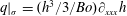
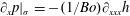
5 Frozen-time linear stability analysis
We have shown in figures 4(a)–4(c) that the quasi-steady buckled-film surface obtained from our periodic simulation loses symmetry roughly at
 $t=7\times 10^{4}$
, when the left secondary trough starts to thin and flatten and the right trough starts to thicken and curve with respect to a fully symmetric simulation. Figure 7(a) represents surface profiles corresponding to this time, as obtained from the periodic (crosses) and symmetric (solid line) simulation, respectively (symmetric data were mirrored onto the full length of the periodic domain). We have checked that both simulations have fully converged in terms of grid resolution (1001 grid points per wavelength
$t=7\times 10^{4}$
, when the left secondary trough starts to thin and flatten and the right trough starts to thicken and curve with respect to a fully symmetric simulation. Figure 7(a) represents surface profiles corresponding to this time, as obtained from the periodic (crosses) and symmetric (solid line) simulation, respectively (symmetric data were mirrored onto the full length of the periodic domain). We have checked that both simulations have fully converged in terms of grid resolution (1001 grid points per wavelength
 $\unicode[STIX]{x1D6EC}$
).
$\unicode[STIX]{x1D6EC}$
).
We now perform a linear stability analysis upon the perfectly symmetric surface profile in figure 7(a) (solid line). We designate this profile as base profile and denote it
 $H(x)$
, neglecting its temporal evolution, which is extremely slow. This amounts to a so-called frozen-time approach. Next, we perturb the base profile infinitesimally, introducing the linear film thickness perturbation
$H(x)$
, neglecting its temporal evolution, which is extremely slow. This amounts to a so-called frozen-time approach. Next, we perturb the base profile infinitesimally, introducing the linear film thickness perturbation
 $h^{\ast }(x,t)$
, which is assumed to grow exponentially:
$h^{\ast }(x,t)$
, which is assumed to grow exponentially:
 $$\begin{eqnarray}h(x,t)=H(x)+h^{\ast }(x,t)=H(x)+{\hat{h}}(x)\exp (\unicode[STIX]{x1D702}t).\end{eqnarray}$$

Figure 7. Frozen-time linear stability analysis of the suspended water film (
 $h_{0}=1~\text{mm}$
,
$h_{0}=1~\text{mm}$
,
 $\mathit{Bo}=0.134$
) at the time of symmetry loss in figure 4(a):
$\mathit{Bo}=0.134$
) at the time of symmetry loss in figure 4(a):
 $t=7\times 10^{4}$
. Open circles mark loci of secondary troughs. (a) Solid line: base state
$t=7\times 10^{4}$
. Open circles mark loci of secondary troughs. (a) Solid line: base state
 $H(x)$
obtained from symmetric simulation on domain of length
$H(x)$
obtained from symmetric simulation on domain of length
 $\unicode[STIX]{x1D6EC}/2$
(501 grid points) and mirrored onto full-wavelength domain; crosses: profile from periodic simulation on domain of length
$\unicode[STIX]{x1D6EC}/2$
(501 grid points) and mirrored onto full-wavelength domain; crosses: profile from periodic simulation on domain of length
 $\unicode[STIX]{x1D6EC}$
(1001 grid points) after loss of symmetry; (b) linear stability results. Solid lines: most-unstable asymmetric (
$\unicode[STIX]{x1D6EC}$
(1001 grid points) after loss of symmetry; (b) linear stability results. Solid lines: most-unstable asymmetric (
 $A_{j}=0$
) and symmetric (
$A_{j}=0$
) and symmetric (
 $B_{j}=0$
) eigenfunctions
$B_{j}=0$
) eigenfunctions
 ${\hat{h}}(x)$
(5.3) obtained from linear stability analysis of the perfectly symmetric profile in (a) (solid line there); asterisks: actual perturbation associated with symmetry loss, i.e. difference between periodic and symmetric profiles in (a); red-dashed line: perturbation resulting from pure translation of base profile
${\hat{h}}(x)$
(5.3) obtained from linear stability analysis of the perfectly symmetric profile in (a) (solid line there); asterisks: actual perturbation associated with symmetry loss, i.e. difference between periodic and symmetric profiles in (a); red-dashed line: perturbation resulting from pure translation of base profile
 $H(x)$
with speed
$H(x)$
with speed
 $c$
, i.e.
$c$
, i.e.
 $\unicode[STIX]{x2202}_{t}h=-c\unicode[STIX]{x2202}_{x}H$
; (c) perturbation profiles from (b) normalized with local film thickness
$\unicode[STIX]{x2202}_{t}h=-c\unicode[STIX]{x2202}_{x}H$
; (c) perturbation profiles from (b) normalized with local film thickness
 $H(x)$
; (d) time derivative of surface curvature
$H(x)$
; (d) time derivative of surface curvature
 $\unicode[STIX]{x2202}_{t}(\unicode[STIX]{x2202}_{xx}h)=\unicode[STIX]{x1D702}\unicode[STIX]{x2202}_{xx}{\hat{h}}$
associated with most-unstable eigenfunctions in (b).
$\unicode[STIX]{x2202}_{t}(\unicode[STIX]{x2202}_{xx}h)=\unicode[STIX]{x1D702}\unicode[STIX]{x2202}_{xx}{\hat{h}}$
associated with most-unstable eigenfunctions in (b).
Upon inserting (5.1) into (2.2) and linearizing in terms of
 ${\hat{h}}$
, an eigenvalue problem with eigenvalue
${\hat{h}}$
, an eigenvalue problem with eigenvalue
 $\unicode[STIX]{x1D702}$
and eigenfunction
$\unicode[STIX]{x1D702}$
and eigenfunction
 ${\hat{h}}$
is obtained:
${\hat{h}}$
is obtained:
 $$\begin{eqnarray}\unicode[STIX]{x1D702}{\hat{h}}=-\unicode[STIX]{x2202}_{x}\left[\frac{H^{3}}{3}\left(\unicode[STIX]{x2202}_{x}{\hat{h}}+\frac{1}{\mathit{Bo}}\unicode[STIX]{x2202}_{xxx}{\hat{h}}\right)+H^{2}\left(\unicode[STIX]{x2202}_{x}H+\frac{1}{\mathit{Bo}}\unicode[STIX]{x2202}_{xxx}H\right){\hat{h}}\right].\end{eqnarray}$$
We choose a Fourier series ansatz with
 $N=100$
for the eigenfunction
$N=100$
for the eigenfunction
 ${\hat{h}}$
:
${\hat{h}}$
:
 $$\begin{eqnarray}{\hat{h}}(x)=\mathop{\sum }_{j=1}^{N}A_{j}\cos (j2\unicode[STIX]{x03C0}x/\unicode[STIX]{x1D6EC})+B_{j}\sin (j2\unicode[STIX]{x03C0}x/\unicode[STIX]{x1D6EC}),\end{eqnarray}$$
and solve the eigenvalue problem with the Galerkin approach (Boyd Reference Boyd1989). We then identify the most-unstable (greatest
 $\unicode[STIX]{x1D702}$
) eigenfunctions for two perturbation types: (i) asymmetric perturbations, when
$\unicode[STIX]{x1D702}$
) eigenfunctions for two perturbation types: (i) asymmetric perturbations, when
 $A_{j}=0$
; and (ii) symmetric perturbations, when
$A_{j}=0$
; and (ii) symmetric perturbations, when
 $B_{j}=0$
.
$B_{j}=0$
.
Figure 7(b) represents the thus obtained eigenfunctions (solid black lines). The asymmetric eigenfunction is associated with a positive eigenvalue
 $\unicode[STIX]{x1D702}=1.8\times 10^{-4}$
. This proves that the film is subject to a symmetry-breaking secondary instability, secondary in the sense that it occurs after the primary Rayleigh–Taylor instability has developed. We call this instability sliding instability. It is associated with a very particular eigenfunction. In fact, the unsymmetric eigenfunction in figure 7(b) is the sole unstable unsymmetric eigenmode. Moreover, it is the sole unstable eigenmode altogether, as all symmetric eigenfunctions are stable, the greatest symmetric eigenvalue being negative
$\unicode[STIX]{x1D702}=1.8\times 10^{-4}$
. This proves that the film is subject to a symmetry-breaking secondary instability, secondary in the sense that it occurs after the primary Rayleigh–Taylor instability has developed. We call this instability sliding instability. It is associated with a very particular eigenfunction. In fact, the unsymmetric eigenfunction in figure 7(b) is the sole unstable unsymmetric eigenmode. Moreover, it is the sole unstable eigenmode altogether, as all symmetric eigenfunctions are stable, the greatest symmetric eigenvalue being negative
 $\unicode[STIX]{x1D702}=-1.9\times 10^{-5}$
(figure 7
b).
$\unicode[STIX]{x1D702}=-1.9\times 10^{-5}$
(figure 7
b).
Crosses in figure 7(b) represent the actual perturbation associated with the loss of symmetry of the periodic simulation. This is easily obtained by taking the difference between the periodic and symmetric surface profiles in figure 7(a). Good agreement in figure 7(b) between the actual perturbation (crosses) and the asymmetric eigenfunction (solid black line) validates both our frozen-time decomposition (5.1) and our Fourier series ansatz (5.3). Validity of the frozen-time approach is further confirmed by the fact that our greatest eigenvalue
 $\unicode[STIX]{x1D702}=1.8\times 10^{-4}$
is an order of magnitude greater than the actual growth rate of the base state at the secondary troughs. We also point out that our stability results have been checked for convergence in terms of
$\unicode[STIX]{x1D702}=1.8\times 10^{-4}$
is an order of magnitude greater than the actual growth rate of the base state at the secondary troughs. We also point out that our stability results have been checked for convergence in terms of
 $N$
in (5.3). Moreover, the same results were obtained independently by the first two authors and were additionally cross-checked by the second author with a pseudo-spectral solver.
$N$
in (5.3). Moreover, the same results were obtained independently by the first two authors and were additionally cross-checked by the second author with a pseudo-spectral solver.
To better understand how the asymmetric eigenfunction
 ${\hat{h}}(x)$
in figure 7(b) affects the base profile
${\hat{h}}(x)$
in figure 7(b) affects the base profile
 $H(x)$
in figure 7(a), we have included an additional curve in figure 7(b). The red-dashed line there represents a pure translation of
$H(x)$
in figure 7(a), we have included an additional curve in figure 7(b). The red-dashed line there represents a pure translation of
 $H(x)$
at constant speed
$H(x)$
at constant speed
 $c$
, in which case the perturbed film thickness would satisfy
$c$
, in which case the perturbed film thickness would satisfy
 $\unicode[STIX]{x2202}_{t}h=-c\unicode[STIX]{x2202}_{x}H$
. It turns out that
$\unicode[STIX]{x2202}_{t}h=-c\unicode[STIX]{x2202}_{x}H$
. It turns out that
 ${\hat{h}}(x)$
corresponds exactly to such a translation within the main hump, as the solid black and red-dashed lines in figure 7(b) collapse there. Differences between the two curves are more apparent when normalizing with the base profile
${\hat{h}}(x)$
corresponds exactly to such a translation within the main hump, as the solid black and red-dashed lines in figure 7(b) collapse there. Differences between the two curves are more apparent when normalizing with the base profile
 $H(x)$
, and this is represented in figure 7(c). We see that the red-dashed and black solid lines almost perfectly coincide within the main hump. This is because the main hump has virtually attained its sinusoidal equilibrium shape of width
$H(x)$
, and this is represented in figure 7(c). We see that the red-dashed and black solid lines almost perfectly coincide within the main hump. This is because the main hump has virtually attained its sinusoidal equilibrium shape of width
 $\unicode[STIX]{x1D6EC}_{c}$
, corresponding to the neutral mode of the Rayleigh–Taylor instability (see § 4). This mode is neutrally stable toward a pure translation and stable toward all other volume-preserving perturbations. Pure translation is thus the only symmetry-breaking option for the main hump and it requires a minimal energy input. It also means that the main hump does not actively contribute to the sliding instability mechanism.
$\unicode[STIX]{x1D6EC}_{c}$
, corresponding to the neutral mode of the Rayleigh–Taylor instability (see § 4). This mode is neutrally stable toward a pure translation and stable toward all other volume-preserving perturbations. Pure translation is thus the only symmetry-breaking option for the main hump and it requires a minimal energy input. It also means that the main hump does not actively contribute to the sliding instability mechanism.
By contrast, at the secondary troughs,
 ${\hat{h}}/H$
, which through (5.1) sets the linear growth rate
${\hat{h}}/H$
, which through (5.1) sets the linear growth rate
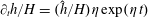 $\unicode[STIX]{x2202}_{t}h/H=({\hat{h}}/H)\unicode[STIX]{x1D702}\exp (\unicode[STIX]{x1D702}\,t)$
, cannot be represented by a pure translation. Such a translation would impose
$\unicode[STIX]{x2202}_{t}h/H=({\hat{h}}/H)\unicode[STIX]{x1D702}\exp (\unicode[STIX]{x1D702}\,t)$
, cannot be represented by a pure translation. Such a translation would impose
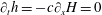 $\unicode[STIX]{x2202}_{t}h=-c\unicode[STIX]{x2202}_{x}H=0$
at the troughs, but our eigenfunction
$\unicode[STIX]{x2202}_{t}h=-c\unicode[STIX]{x2202}_{x}H=0$
at the troughs, but our eigenfunction
 ${\hat{h}}/H$
is clearly non-zero there (open circles in figure 7
c). At the left trough,
${\hat{h}}/H$
is clearly non-zero there (open circles in figure 7
c). At the left trough,
 ${\hat{h}}/H<0$
implying
${\hat{h}}/H<0$
implying
 $\unicode[STIX]{x2202}_{t}h/H<0$
, thus the trough is pushed down and further thins, whereas, at the right trough,
$\unicode[STIX]{x2202}_{t}h/H<0$
, thus the trough is pushed down and further thins, whereas, at the right trough,
 ${\hat{h}}/H>0$
implying
${\hat{h}}/H>0$
implying
 $\unicode[STIX]{x2202}_{t}h/H>0$
, thus the trough is pulled up and further thickens.
$\unicode[STIX]{x2202}_{t}h/H>0$
, thus the trough is pulled up and further thickens.
Closer investigation of the
 ${\hat{h}}/H$
profile in figure 7(c) shows that the film at the trough locus itself is less affected than the immediate surroundings. Indeed, the film is more strongly pushed down to the left of the left trough and more strongly pulled up to the right of the right trough. This tends to move the trough loci leftward, constituting a sliding motion. It also produces a localized surface curvature decrease/increase at the left/right secondary trough. In figure 7(d), we have plotted
${\hat{h}}/H$
profile in figure 7(c) shows that the film at the trough locus itself is less affected than the immediate surroundings. Indeed, the film is more strongly pushed down to the left of the left trough and more strongly pulled up to the right of the right trough. This tends to move the trough loci leftward, constituting a sliding motion. It also produces a localized surface curvature decrease/increase at the left/right secondary trough. In figure 7(d), we have plotted
 $\unicode[STIX]{x1D702}\unicode[STIX]{x2202}_{xx}{\hat{h}}$
, which according to (5.1) is proportional to the time derivative of the perturbed surface curvature
$\unicode[STIX]{x1D702}\unicode[STIX]{x2202}_{xx}{\hat{h}}$
, which according to (5.1) is proportional to the time derivative of the perturbed surface curvature
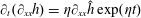 $\unicode[STIX]{x2202}_{t}(\unicode[STIX]{x2202}_{xx}h)=\unicode[STIX]{x1D702}\unicode[STIX]{x2202}_{xx}{\hat{h}}\exp (\unicode[STIX]{x1D702}t)$
. This quantity displays highly localized pulses at the secondary troughs, evidencing a flattening of the left and a curving of the right trough.
$\unicode[STIX]{x2202}_{t}(\unicode[STIX]{x2202}_{xx}h)=\unicode[STIX]{x1D702}\unicode[STIX]{x2202}_{xx}{\hat{h}}\exp (\unicode[STIX]{x1D702}t)$
. This quantity displays highly localized pulses at the secondary troughs, evidencing a flattening of the left and a curving of the right trough.
6 Mechanism of the sliding instability
We seek to identify the positive feedback mechanism causing amplification of the unstable perturbation
 ${\hat{h}}/H$
in figure 7(c) and we focus on the secondary troughs, as the main hump does not actively participate in the instability mechanism (see § 5). Additional evidence for the dynamical importance of the secondary troughs is provided by the transient stability analysis in § 7.
${\hat{h}}/H$
in figure 7(c) and we focus on the secondary troughs, as the main hump does not actively participate in the instability mechanism (see § 5). Additional evidence for the dynamical importance of the secondary troughs is provided by the transient stability analysis in § 7.

Figure 8. Feedback mechanism amplifying the action of the unstable eigenfunction
 ${\hat{h}}$
in figure 7(c). (a) Zoomed view of the base profile
${\hat{h}}$
in figure 7(c). (a) Zoomed view of the base profile
 $H(x)$
(figure 7
a). Open circles mark loci of secondary troughs, asterisks loci of growth rate extrema (e), and the thick red line represents the final equilibrium state (4.1); (b) surface curvature profiles
$H(x)$
(figure 7
a). Open circles mark loci of secondary troughs, asterisks loci of growth rate extrema (e), and the thick red line represents the final equilibrium state (4.1); (b) surface curvature profiles
 $\unicode[STIX]{x2202}_{xx}H$
corresponding to (a). Dashed lines indicate evolution toward equilibrium state; (c) pressure gradient perturbation amplitude according to (6.1a,b
). Solid line: total amplitude
$\unicode[STIX]{x2202}_{xx}H$
corresponding to (a). Dashed lines indicate evolution toward equilibrium state; (c) pressure gradient perturbation amplitude according to (6.1a,b
). Solid line: total amplitude
 $\unicode[STIX]{x2202}_{x}\hat{p}$
; dots: capillary contribution
$\unicode[STIX]{x2202}_{x}\hat{p}$
; dots: capillary contribution
 $\unicode[STIX]{x2202}_{x}\hat{p}|_{\unicode[STIX]{x1D70E}}$
; dot–dashed: gravity-induced contribution
$\unicode[STIX]{x2202}_{x}\hat{p}|_{\unicode[STIX]{x1D70E}}$
; dot–dashed: gravity-induced contribution
 $\unicode[STIX]{x2202}_{x}\hat{p}|_{g}$
; (d) flow rate perturbation amplitude. Solid line: total amplitude
$\unicode[STIX]{x2202}_{x}\hat{p}|_{g}$
; (d) flow rate perturbation amplitude. Solid line: total amplitude
 $\hat{q}$
; dashes: pressure gradient contribution
$\hat{q}$
; dashes: pressure gradient contribution
 $\hat{q}|_{p}=-(1/3)\unicode[STIX]{x2202}_{x}\hat{p}H^{3}$
; dot–dot–dashed: viscous drag contribution
$\hat{q}|_{p}=-(1/3)\unicode[STIX]{x2202}_{x}\hat{p}H^{3}$
; dot–dot–dashed: viscous drag contribution
 $\hat{q}|_{h}=-\unicode[STIX]{x2202}_{x}pH^{2}{\hat{h}}$
; (e) initial growth rate of the perturbation
$\hat{q}|_{h}=-\unicode[STIX]{x2202}_{x}pH^{2}{\hat{h}}$
; (e) initial growth rate of the perturbation
 $\unicode[STIX]{x1D702}{\hat{h}}/H=-\unicode[STIX]{x2202}_{x}\hat{q}$
.
$\unicode[STIX]{x1D702}{\hat{h}}/H=-\unicode[STIX]{x2202}_{x}\hat{q}$
.
Figure 8(a) represents an enlarged view of the buckled portion of the surface profile
 $H(x)$
used for the stability analysis (black line). The thick red line corresponds to the final equilibrium state (4.1) toward which the film evolves by draining the remaining liquid from the secondary hump through the troughs. Drainage is governed by a balance between the driving capillary pressure gradient
$H(x)$
used for the stability analysis (black line). The thick red line corresponds to the final equilibrium state (4.1) toward which the film evolves by draining the remaining liquid from the secondary hump through the troughs. Drainage is governed by a balance between the driving capillary pressure gradient
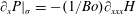 $\unicode[STIX]{x2202}_{x}P|_{\unicode[STIX]{x1D70E}}=-(1/\mathit{Bo})\unicode[STIX]{x2202}_{xxx}H$
, generated through variations in surface curvature
$\unicode[STIX]{x2202}_{x}P|_{\unicode[STIX]{x1D70E}}=-(1/\mathit{Bo})\unicode[STIX]{x2202}_{xxx}H$
, generated through variations in surface curvature
 $\unicode[STIX]{x2202}_{xx}H$
, and viscous drag, which scales with
$\unicode[STIX]{x2202}_{xx}H$
, and viscous drag, which scales with
 $1/H^{3}$
. Because the secondary troughs are so thin, and viscous drag there is so strong, a very steep
$1/H^{3}$
. Because the secondary troughs are so thin, and viscous drag there is so strong, a very steep
 $\unicode[STIX]{x2202}_{xx}H$
profile is established to drive liquid through them. This is plotted with a solid black line in figure 8(b), whereas the thick red line corresponds to the final equilibrium state, with a
$\unicode[STIX]{x2202}_{xx}H$
profile is established to drive liquid through them. This is plotted with a solid black line in figure 8(b), whereas the thick red line corresponds to the final equilibrium state, with a
 $\unicode[STIX]{x2202}_{xx}H$
discontinuity at the juncture of the sinusoidal and zero-thickness film segments (Yiantsios & Higgins Reference Yiantsios and Higgins1989). Dashed lines indicate the evolution toward this state.
$\unicode[STIX]{x2202}_{xx}H$
discontinuity at the juncture of the sinusoidal and zero-thickness film segments (Yiantsios & Higgins Reference Yiantsios and Higgins1989). Dashed lines indicate the evolution toward this state.
Due to the steepness of the base state curvature profile (solid black line in figure 8
b), the localized
 $\unicode[STIX]{x2202}_{xx}{\hat{h}}$
pulses caused by the unstable eigenfunction (figure 7
d) produce large opposite-sign perturbations of the third derivative
$\unicode[STIX]{x2202}_{xx}{\hat{h}}$
pulses caused by the unstable eigenfunction (figure 7
d) produce large opposite-sign perturbations of the third derivative
 $\unicode[STIX]{x2202}_{xxx}{\hat{h}}$
either side of the secondary troughs. These translate into perturbation extrema of the capillary pressure gradient
$\unicode[STIX]{x2202}_{xxx}{\hat{h}}$
either side of the secondary troughs. These translate into perturbation extrema of the capillary pressure gradient
 $\unicode[STIX]{x2202}_{x}\hat{p}|_{\unicode[STIX]{x1D70E}}\propto \unicode[STIX]{x2202}_{xxx}{\hat{h}}$
that destabilize the film, as shown in figure 8(c).
$\unicode[STIX]{x2202}_{x}\hat{p}|_{\unicode[STIX]{x1D70E}}\propto \unicode[STIX]{x2202}_{xxx}{\hat{h}}$
that destabilize the film, as shown in figure 8(c).
In this panel, we have represented the linear response of the driving pressure gradient (4.2) to the perturbed film thickness
 $h$
(5.1):
$h$
(5.1):
 $$\begin{eqnarray}\unicode[STIX]{x2202}_{x}p=\unicode[STIX]{x2202}_{x}P+\unicode[STIX]{x2202}_{x}\hat{p}\exp (\unicode[STIX]{x1D702}t),\quad \unicode[STIX]{x2202}_{x}\hat{p}=\underbrace{-\unicode[STIX]{x2202}_{x}{\hat{h}}}_{\unicode[STIX]{x2202}_{x}\hat{p}|_{g}}-\underbrace{\frac{1}{\mathit{Bo}}\unicode[STIX]{x2202}_{xxx}{\hat{h}}}_{-\unicode[STIX]{x2202}_{x}\hat{p}|_{\unicode[STIX]{x1D70E}}},\end{eqnarray}$$
where, as in (5.1),
 $\unicode[STIX]{x2202}_{x}p$
corresponds to the perturbed quantity,
$\unicode[STIX]{x2202}_{x}p$
corresponds to the perturbed quantity,
 $\unicode[STIX]{x2202}_{x}\hat{p}$
to the perturbation amplitude, and
$\unicode[STIX]{x2202}_{x}\hat{p}$
to the perturbation amplitude, and
 $\unicode[STIX]{x2202}_{x}P$
to the quasi-steady base state. The total perturbation amplitude
$\unicode[STIX]{x2202}_{x}P$
to the quasi-steady base state. The total perturbation amplitude
 $\unicode[STIX]{x2202}_{x}\hat{p}$
is plotted with a solid black line in figure 8(c), whereas the dot–dashed line represents the gravity-induced constituent
$\unicode[STIX]{x2202}_{x}\hat{p}$
is plotted with a solid black line in figure 8(c), whereas the dot–dashed line represents the gravity-induced constituent
 $\unicode[STIX]{x2202}_{x}\hat{p}|_{g}$
, and filled circles the capillary constituent
$\unicode[STIX]{x2202}_{x}\hat{p}|_{g}$
, and filled circles the capillary constituent
 $\unicode[STIX]{x2202}_{x}\hat{p}|_{\unicode[STIX]{x1D70E}}$
. We see that the pressure perturbation is dominated by its capillary contribution
$\unicode[STIX]{x2202}_{x}\hat{p}|_{\unicode[STIX]{x1D70E}}$
. We see that the pressure perturbation is dominated by its capillary contribution
 $\unicode[STIX]{x2202}_{x}\hat{p}|_{\unicode[STIX]{x1D70E}}$
.
$\unicode[STIX]{x2202}_{x}\hat{p}|_{\unicode[STIX]{x1D70E}}$
.
The sign difference of the
 $\unicode[STIX]{x2202}_{x}\hat{p}$
extrema either side of the secondary troughs acts to produce a disparity of flow rate disturbances there. We show this in figure 8(d), which represents the linear response of the flow rate
$\unicode[STIX]{x2202}_{x}\hat{p}$
extrema either side of the secondary troughs acts to produce a disparity of flow rate disturbances there. We show this in figure 8(d), which represents the linear response of the flow rate
 $q=-(h^{3}/3)\unicode[STIX]{x2202}_{x}p$
(4.3) to the perturbed film thickness
$q=-(h^{3}/3)\unicode[STIX]{x2202}_{x}p$
(4.3) to the perturbed film thickness
 $h$
(5.1). The solid line corresponds to the total flow rate perturbation amplitude
$h$
(5.1). The solid line corresponds to the total flow rate perturbation amplitude
 $\hat{q}$
, the dashed line to the contribution of the pressure perturbation
$\hat{q}$
, the dashed line to the contribution of the pressure perturbation
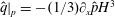 $\hat{q}|_{p}=-(1/3)\unicode[STIX]{x2202}_{x}\hat{p}H^{3}$
and the dot–dot–dashed line to the contribution of the viscous drag perturbation
$\hat{q}|_{p}=-(1/3)\unicode[STIX]{x2202}_{x}\hat{p}H^{3}$
and the dot–dot–dashed line to the contribution of the viscous drag perturbation
 $\hat{q}|_{h}=-\unicode[STIX]{x2202}_{x}pH^{2}{\hat{h}}$
. The effect of the pressure perturbation alone (
$\hat{q}|_{h}=-\unicode[STIX]{x2202}_{x}pH^{2}{\hat{h}}$
. The effect of the pressure perturbation alone (
 $\hat{q}|_{p}$
, dashed line) is to reduce the flow toward the left trough and to increase the flow away from it (note that the base flow rate around the left trough is negative, i.e. to the left), which tends to drive the left trough to thin (and vice versa for the right trough), amplifying the action of the unstable eigenfunction
$\hat{q}|_{p}$
, dashed line) is to reduce the flow toward the left trough and to increase the flow away from it (note that the base flow rate around the left trough is negative, i.e. to the left), which tends to drive the left trough to thin (and vice versa for the right trough), amplifying the action of the unstable eigenfunction
 ${\hat{h}}/H$
. At the same time,
${\hat{h}}/H$
. At the same time,
 ${\hat{h}}/H$
alters the viscous drag around the secondary troughs and this has the opposite effect on the flow rate disturbances (
${\hat{h}}/H$
alters the viscous drag around the secondary troughs and this has the opposite effect on the flow rate disturbances (
 $\hat{q}|_{h}$
, dot–dashed line). Indeed, around the left trough, viscous drag is increased to a greater extent on its left than on its right, and thus the flow away from the trough is reduced more than the flow toward it (the opposite holds at the right trough). However, the net result of the two opposing effects on the total flow rate perturbation
$\hat{q}|_{h}$
, dot–dashed line). Indeed, around the left trough, viscous drag is increased to a greater extent on its left than on its right, and thus the flow away from the trough is reduced more than the flow toward it (the opposite holds at the right trough). However, the net result of the two opposing effects on the total flow rate perturbation
 $\hat{q}$
(solid line) is to increase the flow rate difference across the left trough and to reduce it across the right one.
$\hat{q}$
(solid line) is to increase the flow rate difference across the left trough and to reduce it across the right one.
The spatial variation of
 $\hat{q}$
(solid line in figure 8
d) governs growth and decay of the film thickness through the continuity equation (2.2a
), yielding the growth rate
$\hat{q}$
(solid line in figure 8
d) governs growth and decay of the film thickness through the continuity equation (2.2a
), yielding the growth rate
 $\unicode[STIX]{x1D702}{\hat{h}}/H=-\unicode[STIX]{x2202}_{x}\hat{q}$
, which we have plotted in figure 8(e). Concentrating on the left secondary trough (opposite arguments apply to the right trough), we see that the growth rate minimum is not situated at the trough locus itself but slightly to the left, while there is a smaller local maximum slightly to the right. This has two consequences. First, it causes the trough to move even further to the left, amplifying the action of the
$\unicode[STIX]{x1D702}{\hat{h}}/H=-\unicode[STIX]{x2202}_{x}\hat{q}$
, which we have plotted in figure 8(e). Concentrating on the left secondary trough (opposite arguments apply to the right trough), we see that the growth rate minimum is not situated at the trough locus itself but slightly to the left, while there is a smaller local maximum slightly to the right. This has two consequences. First, it causes the trough to move even further to the left, amplifying the action of the
 ${\hat{h}}/H$
perturbation in figure 7(c). Second, the film is deposited more rapidly on the left of the trough than it is peeled off on the right and this further reduces the local surface curvature, amplifying the action of the
${\hat{h}}/H$
perturbation in figure 7(c). Second, the film is deposited more rapidly on the left of the trough than it is peeled off on the right and this further reduces the local surface curvature, amplifying the action of the
 $\unicode[STIX]{x2202}_{xx}{\hat{h}}$
perturbation in figure 7(d).
$\unicode[STIX]{x2202}_{xx}{\hat{h}}$
perturbation in figure 7(d).
These two positive feedbacks are caused by the way in which the flow rate perturbations in figure 8(d) behave around the trough. The pressure-related perturbation
 $\hat{q}|_{p}$
alone (dashed line) tends to produce a growth rate minimum at the trough locus itself, where
$\hat{q}|_{p}$
alone (dashed line) tends to produce a growth rate minimum at the trough locus itself, where
 $\unicode[STIX]{x2202}_{x}\hat{q}|_{p}$
is strongest. However, the drag-related flow rate perturbation
$\unicode[STIX]{x2202}_{x}\hat{q}|_{p}$
is strongest. However, the drag-related flow rate perturbation
 $\hat{q}|_{h}$
(dot–dot–dashed line) strongly counteracts this effect in the immediate vicinity of the trough, as its slope is opposed. Outside of this region, the relevance of the drag-related perturbation rapidly decays with increasing film thickness (and decreasing magnitude of
$\hat{q}|_{h}$
(dot–dot–dashed line) strongly counteracts this effect in the immediate vicinity of the trough, as its slope is opposed. Outside of this region, the relevance of the drag-related perturbation rapidly decays with increasing film thickness (and decreasing magnitude of
 ${\hat{h}}/H$
). Indeed, while the magnitude of
${\hat{h}}/H$
). Indeed, while the magnitude of
 $\hat{q}|_{p}$
keeps increasing to the left of the left trough, that of
$\hat{q}|_{p}$
keeps increasing to the left of the left trough, that of
 $\hat{q}|_{h}$
slowly decreases after having reached a maximum. This shifts the total growth rate minimum to the left of the trough locus (left-most star in figure 8
e).
$\hat{q}|_{h}$
slowly decreases after having reached a maximum. This shifts the total growth rate minimum to the left of the trough locus (left-most star in figure 8
e).
The growth rate maximum to the right of the left trough (also marked by a star in figure 8
e) occurs for the same reasons. However, it is smaller in magnitude because of the asymmetric shape of the trough region, which connects the steep front of the main hump to the weakly sloped flank of the secondary hump. The thickness of the base state increases more rapidly to the left of the trough than to the right and so the double-pulsed pressure perturbation
 $\unicode[STIX]{x2202}_{x}\hat{p}$
(figure 8
c) unfolds its effect on the flow rate differently on either side (see
$\unicode[STIX]{x2202}_{x}\hat{p}$
(figure 8
c) unfolds its effect on the flow rate differently on either side (see
 $\hat{q}|_{p}$
marked by dashed line in figure 8
d).
$\hat{q}|_{p}$
marked by dashed line in figure 8
d).
Although the engine of the sliding instability is the capillary-induced migration of the secondary troughs, its most-visible consequence is the translation of the main hump, which contains most of the liquid. At first sight, it is surprising that the inconspicuous secondary troughs drive the main hump and not vice versa. However, the main hump has virtually attained a static equilibrium shape (i.e. the cutoff mode of the primary instability) that is neutrally stable toward a pure translation and stable toward all other volume-preserving perturbations. On the one hand, this means that only a minimal driving force is required to move the main hump and thus the latter follows the motion dictated by the secondary troughs. The actual driving force moving the hump results from a capillary pressure difference built up around it by the curvature perturbations in figure 7(d). These induce a greater pressure in the trailing edge of the main hump (left flank in figure 7 a) and a lower one in the leading edge (right flank in figure 7 a). On the other hand, by resisting all other volume-preserving perturbations, the main hump selects the possible sliding instability modes. In particular, the hump’s width is fixed and thus it resists compression/expansion. The two secondary troughs, which in our periodic setting enclose the main hump, are thus required to move in concert in the same direction. They are coupled in that the left one must be perturbed in the exact opposite manner than the right one. This requires the corresponding eigenfunction to be point symmetric about the main hump, a condition satisfied by the unstable mode uncovered in figure 7(c).
7 Transient stability analysis and the onset of sliding
The frozen-time analysis has demonstrated that the film is susceptible to a secondary sliding instability and shed light on the mechanisms involved. However, this method cannot be applied at earlier times when the film evolves more rapidly. Therefore, to investigate the onset of sliding, we relax the assumption of a frozen base state and instead linearize (2.2) around the time-evolving base state
 $H(x,t)$
:
$H(x,t)$
:
 $$\begin{eqnarray}\left.\begin{array}{@{}c@{}}\unicode[STIX]{x2202}_{t}h^{\ast }+\unicode[STIX]{x2202}_{x}q^{\ast }=0,\\ \displaystyle q^{\ast }=\frac{1}{3}H^{3}\left[\unicode[STIX]{x2202}_{x}h^{\ast }+\frac{1}{\mathit{Bo}}\unicode[STIX]{x2202}_{xxx}h^{\ast }\right]+h^{\ast }H^{2}\left[\unicode[STIX]{x2202}_{x}H+\frac{1}{\mathit{Bo}}\unicode[STIX]{x2202}_{xxx}H\right],\end{array}\right\}\end{eqnarray}$$
where
 $h^{\ast }$
and
$h^{\ast }$
and
 $q^{\ast }$
denote the linear perturbations of film thickness and flow rate. We begin by computing the linear noise response of the perfectly symmetrical base state, starting from three representative time points
$q^{\ast }$
denote the linear perturbations of film thickness and flow rate. We begin by computing the linear noise response of the perfectly symmetrical base state, starting from three representative time points
 $t_{i}=1922$
, 20 000 and 70 000 (see figure 3
a to situate
$t_{i}=1922$
, 20 000 and 70 000 (see figure 3
a to situate
 $t_{i}$
in the evolution of the sliding film), for which the profiles
$t_{i}$
in the evolution of the sliding film), for which the profiles
 $H(x,t_{i})$
are plotted in figure 9(a) (a logarithmic ordinate is chosen for better distinction).
$H(x,t_{i})$
are plotted in figure 9(a) (a logarithmic ordinate is chosen for better distinction).

Figure 9. Transient instability and the onset of sliding. (a) Surface profiles
 $H(x,t_{i})$
of the perfectly symmetrical base state at three representative time points (see figure 3
a):
$H(x,t_{i})$
of the perfectly symmetrical base state at three representative time points (see figure 3
a):
 $t_{i}=1922$
(red), 20 000 (green) and 70 000 (blue). A logarithmic ordinate is used for better distinction; (b) long-term linear responses
$t_{i}=1922$
(red), 20 000 (green) and 70 000 (blue). A logarithmic ordinate is used for better distinction; (b) long-term linear responses
 $h^{\ast }(x,t_{i}+T)$
to a noisy perturbation (black line) of the
$h^{\ast }(x,t_{i}+T)$
to a noisy perturbation (black line) of the
 $H(x,t_{i})$
profiles over time horizons
$H(x,t_{i})$
profiles over time horizons
 $T=2000$
(red), 6000 (green) and 10 000 (blue). Solutions to (7.1) while advancing the base state
$T=2000$
(red), 6000 (green) and 10 000 (blue). Solutions to (7.1) while advancing the base state
 $H(x,t)$
from
$H(x,t)$
from
 $t_{i}$
to
$t_{i}$
to
 $t_{i}+T$
; (c) most-unstable perturbations (solid lines) from transient stability analysis (Balestra et al.
Reference Balestra, Brun and Gallaire2016) applied to the
$t_{i}+T$
; (c) most-unstable perturbations (solid lines) from transient stability analysis (Balestra et al.
Reference Balestra, Brun and Gallaire2016) applied to the
 $H(x,t_{i})$
profiles over relatively short time horizons
$H(x,t_{i})$
profiles over relatively short time horizons
 $T=200$
(red) and 1000 (green/blue). Dashed lines represents corresponding responses
$T=200$
(red) and 1000 (green/blue). Dashed lines represents corresponding responses
 $h^{\ast }(x,t_{i}+T)$
, rescaled for a clear comparison; (d) nonlinear response of the periodic simulation in figure 3(a) to an injection of noise
$h^{\ast }(x,t_{i}+T)$
, rescaled for a clear comparison; (d) nonlinear response of the periodic simulation in figure 3(a) to an injection of noise
 $h_{noise}$
(7.6) at
$h_{noise}$
(7.6) at
 $t=683$
. Time traces of the centre of mass
$t=683$
. Time traces of the centre of mass
 $x_{C}$
are represented for different noise levels
$x_{C}$
are represented for different noise levels
 $\unicode[STIX]{x1D700}=\max (h_{noise})-\min (h_{noise})=0$
(solid),
$\unicode[STIX]{x1D700}=\max (h_{noise})-\min (h_{noise})=0$
(solid),
 $1.3\times 10^{-4}$
(dashed),
$1.3\times 10^{-4}$
(dashed),
 $1.3\times 10^{-3}$
(dotted),
$1.3\times 10^{-3}$
(dotted),
 $1.3\times 10^{-2}$
(dot–dashed) and 0.04 (dot–dot–dashed). These correspond to the typical surface roughness of different materials, ranging from glass to steel.
$1.3\times 10^{-2}$
(dot–dashed) and 0.04 (dot–dot–dashed). These correspond to the typical surface roughness of different materials, ranging from glass to steel.
We solve (7.1) for
 $h^{\ast }(x,t)$
, starting from a noisy initial condition
$h^{\ast }(x,t)$
, starting from a noisy initial condition
 $h^{\ast }(x,t_{i})=h_{noise}$
(defined in (7.6) and represented by a black line in figure 9
b), while advancing
$h^{\ast }(x,t_{i})=h_{noise}$
(defined in (7.6) and represented by a black line in figure 9
b), while advancing
 $H(x,t)$
from
$H(x,t)$
from
 $t=t_{i}$
to
$t=t_{i}$
to
 $t=t_{i}+T$
over a relatively long time horizon
$t=t_{i}+T$
over a relatively long time horizon
 $T$
(see caption of figure 11). Coloured lines in figure 9(b) represent the obtained linear responses
$T$
(see caption of figure 11). Coloured lines in figure 9(b) represent the obtained linear responses
 $h^{\ast }(x,t_{i}+T)$
. For all three cases, the noisy initial perturbation evolves into a sliding mode similar to the eigenfunction obtained with the frozen-time approach (see figure 7
b). The growth rate is largest for the earliest (red line,
$h^{\ast }(x,t_{i}+T)$
. For all three cases, the noisy initial perturbation evolves into a sliding mode similar to the eigenfunction obtained with the frozen-time approach (see figure 7
b). The growth rate is largest for the earliest (red line,
 $t_{i}=1922$
) and lowest for the latest (blue line,
$t_{i}=1922$
) and lowest for the latest (blue line,
 $t_{i}=70\,000$
) base state profile
$t_{i}=70\,000$
) base state profile
 $H(x,t_{i})$
.
$H(x,t_{i})$
.
Next, we follow the transient stability analysis outlined in Balestra et al. (Reference Balestra, Brun and Gallaire2016) (see also Schmid Reference Schmid2007) to identify the most-unstable perturbations associated with the base state profiles
 $H(x,t_{i})$
. We repeatedly solve the direct problem (7.1) from an iteratively improved initial condition:
$H(x,t_{i})$
. We repeatedly solve the direct problem (7.1) from an iteratively improved initial condition:
 $$\begin{eqnarray}h^{\ast }(x,t_{i})=\frac{1}{2}h^{\dagger }(x,t_{i})G(T)\int _{0}^{L}h_{old}^{\ast }(x,t_{i})^{2}\,\text{d}x,\end{eqnarray}$$
obtained by solving the adjoint problem:
 $$\begin{eqnarray}\left.\begin{array}{@{}c@{}}\displaystyle \unicode[STIX]{x2202}_{t}h^{\dagger }-\frac{1}{3}\left[\unicode[STIX]{x2202}_{x}(qH^{3})+\frac{1}{\mathit{Bo}}\unicode[STIX]{x2202}_{xxx}(qH^{3})\right]+qH^{2}\left[\unicode[STIX]{x2202}_{x}H+\frac{1}{\mathit{Bo}}\unicode[STIX]{x2202}_{xxx}H\right]=0,\\ \displaystyle q=\unicode[STIX]{x2202}_{x}h^{\dagger },\end{array}\right\}\end{eqnarray}$$
starting from the end condition:
 $$\begin{eqnarray}h^{\dagger }(x,t_{i}+T)=2\frac{h^{\ast }(x,t_{i}+T)}{\displaystyle \int _{0}^{L}h^{\ast }(x,t_{i})^{2}\,\text{d}x},\end{eqnarray}$$
and stepping backwards in time from
 $t_{i}+T$
to
$t_{i}+T$
to
 $t_{i}$
. The procedure converges to a maximal value of the gain
$t_{i}$
. The procedure converges to a maximal value of the gain
 $G(T)$
:
$G(T)$
:
 $$\begin{eqnarray}G(T)=\frac{\displaystyle \int _{0}^{L}h^{\ast }(x,t_{i})^{2}\,\text{d}x}{\displaystyle \int _{0}^{L}h^{\ast }(x,t_{i}+T)^{2}\,\text{d}x},\end{eqnarray}$$
which quantifies growth over the time horizon
 $T$
. Figure 9(c) represents the thus-obtained most-unstable perturbations
$T$
. Figure 9(c) represents the thus-obtained most-unstable perturbations
 $h^{\ast }(x,t_{i})$
for the three base state profiles
$h^{\ast }(x,t_{i})$
for the three base state profiles
 $H(x,t_{i})$
in figure 9(a) over relatively short time horizons
$H(x,t_{i})$
in figure 9(a) over relatively short time horizons
 $T$
(see caption).
$T$
(see caption).
All
 $h^{\ast }(x,t_{i})$
profiles display localized pulses that respectively thin and thicken the two secondary troughs. Over the time horizon
$h^{\ast }(x,t_{i})$
profiles display localized pulses that respectively thin and thicken the two secondary troughs. Over the time horizon
 $T$
, they all evolve toward the sliding eigenmode obtained with our frozen-time analysis (5.1), as shown by the dashed lines in figure 11(c), which represent the linear responses
$T$
, they all evolve toward the sliding eigenmode obtained with our frozen-time analysis (5.1), as shown by the dashed lines in figure 11(c), which represent the linear responses
 $h^{\ast }(x,t_{i}+T)$
. Thus, the most-unstable scenario identified through our transient analysis exhibits the same long-time asymptotic behaviour, i.e. a concerted sliding motion of the entire film. This sliding eigenmode, which grows in a shape-preserving form, is most-effectively triggered by localized asymmetric disturbances at the secondary troughs, highlighting the importance of these regions for the onset of sliding.
$h^{\ast }(x,t_{i}+T)$
. Thus, the most-unstable scenario identified through our transient analysis exhibits the same long-time asymptotic behaviour, i.e. a concerted sliding motion of the entire film. This sliding eigenmode, which grows in a shape-preserving form, is most-effectively triggered by localized asymmetric disturbances at the secondary troughs, highlighting the importance of these regions for the onset of sliding.
Applying the transient analysis at earlier times, we have observed a qualitative change in the behaviour of the film near the time of buckling. In the pre-buckling regime, the most-unstable disturbance corresponds to a pure translation that merely produces a phase shift in the evolving film. It is only after buckling has occurred that the most-unstable disturbance mode takes on the non-trivial, localized form shown in figure 9(c). Thereafter, it remains virtually unchanged in form, with a gain
 $G(T)$
that is always greater than unity. In fact, we find that
$G(T)$
that is always greater than unity. In fact, we find that
 $G(T)$
is lower for later
$G(T)$
is lower for later
 $t_{i}$
, which is probably due to the increase in viscous stresses. Thus, there is no intrinsic/inherent fixed time for the onset of sliding. Rather, the onset of a macroscopically visible sliding motion is controlled by the level of ambient noise, e.g. due to surface roughness or pressure fluctuations. To demonstrate this, we have solved our nonlinear model (2.2), subject to periodic boundary conditions and starting from the initial condition (2.4), while injecting synthetic noise at a specific time
$t_{i}$
, which is probably due to the increase in viscous stresses. Thus, there is no intrinsic/inherent fixed time for the onset of sliding. Rather, the onset of a macroscopically visible sliding motion is controlled by the level of ambient noise, e.g. due to surface roughness or pressure fluctuations. To demonstrate this, we have solved our nonlinear model (2.2), subject to periodic boundary conditions and starting from the initial condition (2.4), while injecting synthetic noise at a specific time
 $t_{noise}=683$
, i.e. just after the film surface has buckled (see figure 3
a). This is done through the random film thickness perturbation
$t_{noise}=683$
, i.e. just after the film surface has buckled (see figure 3
a). This is done through the random film thickness perturbation
 $h_{noise}$
(Chang, Demekhin & Kalaidin Reference Chang, Demekhin and Kalaidin1996):
$h_{noise}$
(Chang, Demekhin & Kalaidin Reference Chang, Demekhin and Kalaidin1996):
 $$\begin{eqnarray}h_{noise}=\unicode[STIX]{x1D716}\mathop{\sum }_{j=1}^{N}\cos (j\unicode[STIX]{x0394}kx-\unicode[STIX]{x1D711}_{rand}),\quad \unicode[STIX]{x0394}k=100k_{c}/N,\,k_{c}=\sqrt{\mathit{Bo}},\end{eqnarray}$$
which consists of sinusoidal modes of random phase shift
 $\unicode[STIX]{x1D711}_{rand}$
that cover 100 times the unstable range of the primary instability. By changing the coefficient
$\unicode[STIX]{x1D711}_{rand}$
that cover 100 times the unstable range of the primary instability. By changing the coefficient
 $\unicode[STIX]{x1D716}$
, the noise level
$\unicode[STIX]{x1D716}$
, the noise level
 $\unicode[STIX]{x1D700}=\max (h_{noise})-\min (h_{noise})$
was varied in five simulation runs:
$\unicode[STIX]{x1D700}=\max (h_{noise})-\min (h_{noise})$
was varied in five simulation runs:
 $\unicode[STIX]{x1D700}=0$
,
$\unicode[STIX]{x1D700}=0$
,
 $1.3\times 10^{-4}$
,
$1.3\times 10^{-4}$
,
 $1.3\times 10^{-3}$
,
$1.3\times 10^{-3}$
,
 $1.3\times 10^{-2}$
and 0.04. These values correspond to the typical surface roughness of different materials, ranging from glass to steel. Figure 9(d) represents time traces of the position
$1.3\times 10^{-2}$
and 0.04. These values correspond to the typical surface roughness of different materials, ranging from glass to steel. Figure 9(d) represents time traces of the position
 $x_{C}$
of the film’s centre of mass (initially in the middle of the domain, i.e.
$x_{C}$
of the film’s centre of mass (initially in the middle of the domain, i.e.
 $x_{C}/L=0.5$
), as obtained from the five runs. The onset of sliding is considerably precipitated with increasing noise level but, in the range studied, always occurs in the quasi-steady regime of the base state (
$x_{C}/L=0.5$
), as obtained from the five runs. The onset of sliding is considerably precipitated with increasing noise level but, in the range studied, always occurs in the quasi-steady regime of the base state (
 $t\geqslant 2\times 10^{-4}$
, see figure 3
a). Thus, although linear theory suggests that the film is susceptible to sliding at any time after buckling, nonlinearly, we find that the sliding eigenmode is only able to emerge after the film has slowed down to a quasi-steady state with quasi-equilibrium humps and sharp secondary troughs.
$t\geqslant 2\times 10^{-4}$
, see figure 3
a). Thus, although linear theory suggests that the film is susceptible to sliding at any time after buckling, nonlinearly, we find that the sliding eigenmode is only able to emerge after the film has slowed down to a quasi-steady state with quasi-equilibrium humps and sharp secondary troughs.
8 Gas film underneath a liquid layer
The ingredients of the sliding instability, identified for a suspended liquid film in § 6, are quite general and can be found in other systems as well, albeit in the presence of additional effects that may call for more complex models. One such scenario, which involves two active fluid phases, is related to the spontaneous motion of Leidenfrost drops on a heated surface. Liquid in contact with the hot surface evaporates to form a thin vapour film that supports the drop. Burton et al. (Reference Burton, Sharpe, van der Veen, Franco and Nagel2012) measured the vapour film underneath a Leidenfrost drop made of water and showed that the vapour–liquid interface is buckled, similar to what we have observed in figure 3(d) for the suspended water film. In a follow-up paper, Ma et al. (Reference Ma, Liétor-Santos and Burton2015) mention that the smooth aluminium substrate heating their Leidenfrost drop was curved ‘in order to keep drops stationary and suppress the buoyancy-driven Rayleigh–Taylor instability in the vapor layer’. They also contend that the dynamical traits of Leidenfrost drops, such as self-propulsion (Linke et al.
Reference Linke, Alemán, Melling, Taormina, Francis, Dow-Hygelund, Narayanan, Taylor and Stout2006; Quéré Reference Quéré2013), depend ‘on a sensitive coupling between deformations of the liquid/vapor interface and lubrication flow in the thin (
 ${\approx}100~\unicode[STIX]{x03BC}\text{m}$
) vapor layer’. Most recently, experiments of Ma, Liétor-Santos & Burton (Reference Ma, Liétor-Santos and Burton2017) have shown that the oscillatory dynamics of Leidenfrost drops, which is linked to the drainage of vapour below the drop, depends only on the capillary length of the liquid, ‘indicating a purely hydrodynamic (non-thermal) origin for the oscillations’.
${\approx}100~\unicode[STIX]{x03BC}\text{m}$
) vapor layer’. Most recently, experiments of Ma, Liétor-Santos & Burton (Reference Ma, Liétor-Santos and Burton2017) have shown that the oscillatory dynamics of Leidenfrost drops, which is linked to the drainage of vapour below the drop, depends only on the capillary length of the liquid, ‘indicating a purely hydrodynamic (non-thermal) origin for the oscillations’.

Figure 10. Spontaneous sliding of a very thin gas film underneath a liquid layer (see sketch in figure 1
b), as simulated with the full model (2.1). Fluid properties (see caption of figure 1
b for values) correspond to a water vapour film underneath a water drop, according to the experiments of Burton et al. (Reference Burton, Sharpe, van der Veen, Franco and Nagel2012). The mean film thickness is
 $h_{0}=100~\unicode[STIX]{x03BC}\text{m}$
and the Bond number
$h_{0}=100~\unicode[STIX]{x03BC}\text{m}$
and the Bond number
 $\mathit{Bo}=0.0016$
. The domain length corresponds to the most-amplified wavelength of the Rayleigh–Taylor instability
$\mathit{Bo}=0.0016$
. The domain length corresponds to the most-amplified wavelength of the Rayleigh–Taylor instability
 $\unicode[STIX]{x1D6EC}=2\sqrt{2}\unicode[STIX]{x03C0}/\sqrt{\mathit{Bo}}$
. (a) Logarithmic profiles of the film surface. Solid lines: profiles just before and after the onset of sliding; circles: suspended water film from figure 3; (b) film thickness time traces at the left and right secondary troughs. Solid: full model (2.1), dashed: full model in the limit
$\unicode[STIX]{x1D6EC}=2\sqrt{2}\unicode[STIX]{x03C0}/\sqrt{\mathit{Bo}}$
. (a) Logarithmic profiles of the film surface. Solid lines: profiles just before and after the onset of sliding; circles: suspended water film from figure 3; (b) film thickness time traces at the left and right secondary troughs. Solid: full model (2.1), dashed: full model in the limit
 $\unicode[STIX]{x1D6F1}_{\unicode[STIX]{x1D707}}\rightarrow 0$
, dot–dot–dashed: simplified model (2.2).
$\unicode[STIX]{x1D6F1}_{\unicode[STIX]{x1D707}}\rightarrow 0$
, dot–dot–dashed: simplified model (2.2).
These experimental observations have prompted us to check whether a vapour film underneath a liquid layer, such as illustrated in figure 1(b), is prone to the sliding instability in a purely hydrodynamical sense, i.e. without accounting for evaporation. We consider the parameters quantified in the caption of figure 1(b), which are based on the experiments of Burton et al. (Reference Burton, Sharpe, van der Veen, Franco and Nagel2012), i.e. the gas layer consists of water vapour and the liquid layer of liquid water. The physical properties of the liquid (
 $\unicode[STIX]{x1D707}_{2}$
,
$\unicode[STIX]{x1D707}_{2}$
,
 $\unicode[STIX]{x1D70C}_{2}$
) and the surface tension
$\unicode[STIX]{x1D70C}_{2}$
) and the surface tension
 $\unicode[STIX]{x1D70E}$
were evaluated at the experimental saturation temperature
$\unicode[STIX]{x1D70E}$
were evaluated at the experimental saturation temperature
 $T=100\,^{\circ }\text{C}$
, whereas the vapour properties (
$T=100\,^{\circ }\text{C}$
, whereas the vapour properties (
 $\unicode[STIX]{x1D707}_{1}$
,
$\unicode[STIX]{x1D707}_{1}$
,
 $\unicode[STIX]{x1D70C}_{1}$
) were evaluated at
$\unicode[STIX]{x1D70C}_{1}$
) were evaluated at
 $T=235\,^{\circ }\text{C}$
, corresponding to the average between the experimental wall and saturation temperatures. The mean vapour thickness was set to
$T=235\,^{\circ }\text{C}$
, corresponding to the average between the experimental wall and saturation temperatures. The mean vapour thickness was set to
 $h_{0}=100~\unicode[STIX]{x03BC}\text{m}$
, yielding a Bond number of
$h_{0}=100~\unicode[STIX]{x03BC}\text{m}$
, yielding a Bond number of
 $\mathit{Bo}=0.0016$
comparable to the experiments.
$\mathit{Bo}=0.0016$
comparable to the experiments.
We have performed a periodic simulation of this configuration with our full model (2.1), which accounts for coupling between the thin gas film and the much more viscous liquid phase, the viscosity ratio being
 $\unicode[STIX]{x1D6F1}_{\unicode[STIX]{x1D707}}=2\times 10^{3}$
. The domain length was set to
$\unicode[STIX]{x1D6F1}_{\unicode[STIX]{x1D707}}=2\times 10^{3}$
. The domain length was set to
 $\unicode[STIX]{x1D6EC}=2\sqrt{2}\unicode[STIX]{x03C0}/\sqrt{\mathit{Bo}}$
(the most-amplified wavelength of the Rayleigh–Taylor instability) and its height
$\unicode[STIX]{x1D6EC}=2\sqrt{2}\unicode[STIX]{x03C0}/\sqrt{\mathit{Bo}}$
(the most-amplified wavelength of the Rayleigh–Taylor instability) and its height
 $D=10$
was chosen so large that the liquid phase is quasi-unconfined.
$D=10$
was chosen so large that the liquid phase is quasi-unconfined.
Our simulation has shown that the vapour film indeed slides spontaneously, displaying all the characteristic features of the sliding instability identified in § 6. Figure 10(a) represents the vapour film surface at two characteristic time points, just before and somewhat after the onset of sliding. We have additionally included a profile of the suspended water film from § 3 just before it slides (symbols in figure 10
a). We have chosen logarithmic scaling on the ordinate to accentuate any differences between the vapour film and the suspended water film. At the sliding onset, the surface profiles for the two cases, which have been scaled horizontally with the domain length
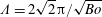 $\unicode[STIX]{x1D6EC}=2\sqrt{2}\unicode[STIX]{x03C0}/\sqrt{\mathit{Bo}}$
, are virtually identical. This follows from capillary pressure gradients dominating the long-time evolution of the film, in which case (2.2) reduces to
$\unicode[STIX]{x1D6EC}=2\sqrt{2}\unicode[STIX]{x03C0}/\sqrt{\mathit{Bo}}$
, are virtually identical. This follows from capillary pressure gradients dominating the long-time evolution of the film, in which case (2.2) reduces to
 $\unicode[STIX]{x2202}_{t}h\propto \unicode[STIX]{x2202}_{x}(h^{3}\unicode[STIX]{x2202}_{xxx}h)$
after rescaling the horizontal coordinate
$\unicode[STIX]{x2202}_{t}h\propto \unicode[STIX]{x2202}_{x}(h^{3}\unicode[STIX]{x2202}_{xxx}h)$
after rescaling the horizontal coordinate
 $x$
with
$x$
with
 $\unicode[STIX]{x1D6EC}$
and adjusting the time scale accordingly.
$\unicode[STIX]{x1D6EC}$
and adjusting the time scale accordingly.
The sliding onset for the vapour film is discernible in figure 10(b), showing time traces of the film thickness at the two secondary troughs. The role of viscous coupling is evidenced by comparing the full-model prediction (2.1) (solid line) with the limit
 $\unicode[STIX]{x1D6F1}_{\unicode[STIX]{x1D707}}\rightarrow 0$
(dashed line). Viscous stresses in the outer phase, through their action at the gas–liquid interface, modify the velocity profile and the associated viscous drag within the gas film. As a result, the onset of sliding is significantly delayed. These stresses also suppress the inertia-induced oscillation of the secondary troughs which had been observed for the suspended water film in figure 3(b) and figure 5. However, they do not qualitatively alter the loss of symmetry and sliding. In figure 10(b), we have also included the prediction of the simplified model (2.2) for completeness (see dot–dot–dashed line).
$\unicode[STIX]{x1D6F1}_{\unicode[STIX]{x1D707}}\rightarrow 0$
(dashed line). Viscous stresses in the outer phase, through their action at the gas–liquid interface, modify the velocity profile and the associated viscous drag within the gas film. As a result, the onset of sliding is significantly delayed. These stresses also suppress the inertia-induced oscillation of the secondary troughs which had been observed for the suspended water film in figure 3(b) and figure 5. However, they do not qualitatively alter the loss of symmetry and sliding. In figure 10(b), we have also included the prediction of the simplified model (2.2) for completeness (see dot–dot–dashed line).
Our simplified analysis is far from proving that the sliding instability is linked to the spontaneous motion of Leidenfrost drops. Nonetheless, it has identified a possible mechanism. To verify whether this mechanism holds underneath a Leidenfrost drop, further analysis needs to include evaporation. The effect of evaporation may be stabilizing in that it tends to thicken a trough that has been thinned by a perturbation. On the other hand, it creates additional fluid within the secondary hump that needs to be drained through the troughs and this should be destabilizing. Evaporation maintains the interface at uniform temperature. This precludes the development of Marangoni stresses, which normally play a key role in the evolution of heated films. This is the subject of the next section, in which we show that such stresses can suppress the sliding instability.
9 Suppression of sliding by Marangoni stresses
Let us revisit the suspended liquid film in figure 1(a), but with the wall at a higher temperature than the ambient passive gas. Then modulations of the film thickness will result in temperature variations along the interface, which will in turn produce thermal Marangoni stresses. Since they act along the interface, the effect of these stresses on fluid drainage will be very different from that of capillary pressure gradients, which act within the bulk of the fluid. In fact, as we will show, these stresses can completely suppress sliding provided the wall is sufficiently hot.
In this analysis, we assume that surface tension decreases with temperature,
 $\unicode[STIX]{x2202}_{T}\unicode[STIX]{x1D70E}<0$
, in which case the problem is governed by (2.3), where the modified Marangoni number
$\unicode[STIX]{x2202}_{T}\unicode[STIX]{x1D70E}<0$
, in which case the problem is governed by (2.3), where the modified Marangoni number
 $\mathit{Ma}=\unicode[STIX]{x2202}_{T}\unicode[STIX]{x1D70E}(T_{w}-T_{\infty })/\unicode[STIX]{x1D70E}$
is negative. The Marangoni effect is thus destabilizing in terms of the primary instability. We have performed periodic simulations of (2.3) using the same parameter values as in § 3 (see caption of figure 1
a), additionally setting the Biot number to
$\mathit{Ma}=\unicode[STIX]{x2202}_{T}\unicode[STIX]{x1D70E}(T_{w}-T_{\infty })/\unicode[STIX]{x1D70E}$
is negative. The Marangoni effect is thus destabilizing in terms of the primary instability. We have performed periodic simulations of (2.3) using the same parameter values as in § 3 (see caption of figure 1
a), additionally setting the Biot number to
 $\mathit{Bi}=1$
and increasing the magnitude of
$\mathit{Bi}=1$
and increasing the magnitude of
 $\mathit{Ma}<0$
step by step from zero.
$\mathit{Ma}<0$
step by step from zero.
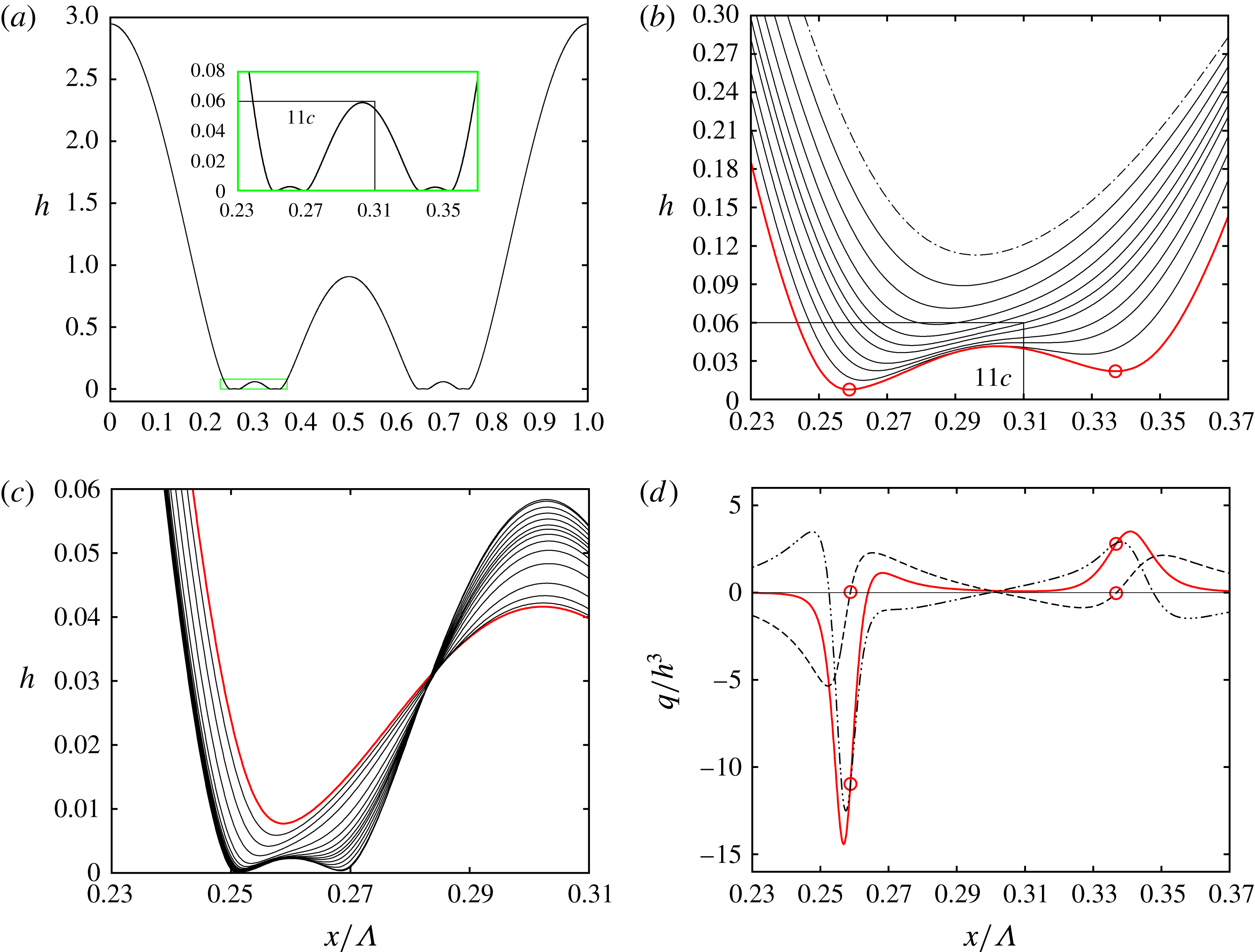
Figure 11. Suppression of sliding by thermal Marangoni stresses. Heating the suspended water film from the wall suppresses the sliding instability and instead causes a cascade of buckling events (see also supplementary movie 3) similar to the traditional Marangoni problem (Boos & Thess Reference Boos and Thess1999; Oron Reference Oron2000). Numerical simulation of (2.3) using
 $\mathit{Ma}=-0.2$
,
$\mathit{Ma}=-0.2$
,
 $\mathit{Bi}=1.0$
and
$\mathit{Bi}=1.0$
and
 $\mathit{Bo}=0.134$
(see caption of figure 1
a for other quantities). (a) Surface profile after three buckling events (
$\mathit{Bo}=0.134$
(see caption of figure 1
a for other quantities). (a) Surface profile after three buckling events (
 $t=2\times 10^{4}$
). Inset shows enlarged view of boxed region around left tertiary hump; (b) formation of left tertiary hump from second buckling event; (c) formation of left-most quaternary hump (boxed region in inset of (a)) from third buckling event; (d) flow rate contributions (9.1) (normalized with
$t=2\times 10^{4}$
). Inset shows enlarged view of boxed region around left tertiary hump; (b) formation of left tertiary hump from second buckling event; (c) formation of left-most quaternary hump (boxed region in inset of (a)) from third buckling event; (d) flow rate contributions (9.1) (normalized with
 $h^{3}$
) corresponding to the thick red profile in (b). Open circles mark loci of tertiary troughs. Thick red solid line: total flow rate
$h^{3}$
) corresponding to the thick red profile in (b). Open circles mark loci of tertiary troughs. Thick red solid line: total flow rate
 $q$
; dashed: thermocapillary contribution
$q$
; dashed: thermocapillary contribution
 $q|_{\mathit{Ma}}$
; dot–dot–dashed: capillary contribution
$q|_{\mathit{Ma}}$
; dot–dot–dashed: capillary contribution
 $q|_{\unicode[STIX]{x1D70E}}$
. Thick red profiles all correspond to same time.
$q|_{\unicode[STIX]{x1D70E}}$
. Thick red profiles all correspond to same time.
Our simulations have shown that sliding is suppressed above a certain threshold value for
 $|\mathit{Ma}|$
. Instead of sliding, the film undergoes a cascade of buckling events that constantly produce new generations of humps and associated troughs, as has been observed in the traditional Marangoni problem (Boos & Thess Reference Boos and Thess1999; Oron Reference Oron2000). We focus our remaining discussion on a representative simulation for
$|\mathit{Ma}|$
. Instead of sliding, the film undergoes a cascade of buckling events that constantly produce new generations of humps and associated troughs, as has been observed in the traditional Marangoni problem (Boos & Thess Reference Boos and Thess1999; Oron Reference Oron2000). We focus our remaining discussion on a representative simulation for
 $\mathit{Ma}=-0.2$
, results of which are plotted in figure 11. We have also provided a supplementary movie, movie 3, which shows the buckling cascade in action (therein, the ordinate has been scaled logarithmically to highlight the evolution of the troughs).
$\mathit{Ma}=-0.2$
, results of which are plotted in figure 11. We have also provided a supplementary movie, movie 3, which shows the buckling cascade in action (therein, the ordinate has been scaled logarithmically to highlight the evolution of the troughs).
Figure 11(a) represents the film surface after three buckling events. The inset shows an enlarged view of the boxed region surrounding the left tertiary hump, which results from the second buckling event. Figure 11(b) displays the time evolution of this second buckling event, from the dot–dashed unbuckled profile to the thick red profile, where the tertiary hump and associated troughs have already formed. Subsequently, the tertiary troughs (marked by open circles in figure 11 b) undergo a third buckling event, forming quaternary humps and troughs. This is shown in figure 11(c) for the left-most tertiary trough.
We now focus on the thick red profile in figure 11(b), which results from the second buckling event, and evaluate the different flow rate contributions:
 $$\begin{eqnarray}q=q|_{g}+q|_{\unicode[STIX]{x1D70E}}-\underbrace{\frac{1}{2}\frac{\mathit{Ma}}{\mathit{Bo}}h^{2}\unicode[STIX]{x2202}_{x}h\frac{\mathit{Bi}}{(1+\mathit{Bi}\,h)^{2}}}_{-q|_{\mathit{Ma}}},\end{eqnarray}$$
where
 $q|_{\mathit{Ma}}$
denotes the contribution due to Marangoni stresses and
$q|_{\mathit{Ma}}$
denotes the contribution due to Marangoni stresses and
 $q|_{g}$
and
$q|_{g}$
and
 $q|_{\unicode[STIX]{x1D70E}}$
are defined according to (4.3). These contributions are plotted in figure 11(d), where we have normalized
$q|_{\unicode[STIX]{x1D70E}}$
are defined according to (4.3). These contributions are plotted in figure 11(d), where we have normalized
 $q$
with
$q$
with
 $h^{3}$
. The thick red line corresponds to the total flow rate
$h^{3}$
. The thick red line corresponds to the total flow rate
 $q$
, the dot–dot–dashed line to the capillary contribution
$q$
, the dot–dot–dashed line to the capillary contribution
 $q|_{\unicode[STIX]{x1D70E}}$
, and the dashed line to the thermocapillary contribution
$q|_{\unicode[STIX]{x1D70E}}$
, and the dashed line to the thermocapillary contribution
 $q|_{\mathit{Ma}}$
, while
$q|_{\mathit{Ma}}$
, while
 $q|_{g}$
is negligible and thus not plotted.
$q|_{g}$
is negligible and thus not plotted.
Considering the region around the left tertiary trough (left-most open circles in figures 11
b and 11
d), we see that the thermocapillary contribution
 $q|_{\mathit{Ma}}$
(dashed line in figure 11
d) is significant compared to the capillary one (dot–dot–dashed line). In contrast to the isothermal case in figure 6(h), drainage is thus not dominated by variations in surface curvature
$q|_{\mathit{Ma}}$
(dashed line in figure 11
d) is significant compared to the capillary one (dot–dot–dashed line). In contrast to the isothermal case in figure 6(h), drainage is thus not dominated by variations in surface curvature
 $\unicode[STIX]{x2202}_{xx}h$
. Instead, the surface slope
$\unicode[STIX]{x2202}_{xx}h$
. Instead, the surface slope
 $\unicode[STIX]{x2202}_{x}h$
, which determines
$\unicode[STIX]{x2202}_{x}h$
, which determines
 $q|_{\mathit{Ma}}$
in (9.1), also plays an important role. We have verified that this holds for subsequent buckling events.
$q|_{\mathit{Ma}}$
in (9.1), also plays an important role. We have verified that this holds for subsequent buckling events.
The reason
 $q|_{\mathit{Ma}}$
remains relevant even when the film is very thin, in contrast to
$q|_{\mathit{Ma}}$
remains relevant even when the film is very thin, in contrast to
 $q|_{g}$
(4.3) which is also proportional to
$q|_{g}$
(4.3) which is also proportional to
 $\unicode[STIX]{x2202}_{x}h$
but subsides after producing the first buckling event (see figure 6), is that it scales with
$\unicode[STIX]{x2202}_{x}h$
but subsides after producing the first buckling event (see figure 6), is that it scales with
 $h^{2}$
instead of
$h^{2}$
instead of
 $h^{3}$
. The Marangoni effect, which acts at the film surface, is less hindered by viscous drag.
$h^{3}$
. The Marangoni effect, which acts at the film surface, is less hindered by viscous drag.
Thermocapillary drainage
 $q|_{\mathit{Ma}}\propto \unicode[STIX]{x2202}_{x}h$
is fundamentally different from capillary drainage in that it is symmetric about the troughs (where
$q|_{\mathit{Ma}}\propto \unicode[STIX]{x2202}_{x}h$
is fundamentally different from capillary drainage in that it is symmetric about the troughs (where
 $\unicode[STIX]{x2202}_{x}h=0$
). That is, liquid underneath a trough is driven away to both sides, as evidenced by the profile of
$\unicode[STIX]{x2202}_{x}h=0$
). That is, liquid underneath a trough is driven away to both sides, as evidenced by the profile of
 $q|_{\mathit{Ma}}$
(dashed line) around the left-most tertiary trough in figure 11(d). Marangoni stresses thus help capillary drainage on one side of a trough and counteract it on the other and this is responsible for both the buckling cascade and the suppression of sliding.
$q|_{\mathit{Ma}}$
(dashed line) around the left-most tertiary trough in figure 11(d). Marangoni stresses thus help capillary drainage on one side of a trough and counteract it on the other and this is responsible for both the buckling cascade and the suppression of sliding.
Closer investigation of figures 11(b) and 11(c) shows that the buckling events from the second one onward differ from the first buckling event (figure 3
d) in that the buckling trough does not split into two new identical daughter troughs on either side. Instead, a new trough forms always on the inside of the original trough, which itself moves outward. This follows from the competition between thermocapillary
 $q|_{\mathit{Ma}}$
and capillary
$q|_{\mathit{Ma}}$
and capillary
 $q|_{\unicode[STIX]{x1D70E}}$
drainage, which produces a divergence point (
$q|_{\unicode[STIX]{x1D70E}}$
drainage, which produces a divergence point (
 $q=0$
) to the right of the left-most tertiary trough in figure 11(d) (see thick red line). From this divergence point, liquid is drained to either side, ultimately producing a quaternary trough there, when the slope of the secondary hump
$q=0$
) to the right of the left-most tertiary trough in figure 11(d) (see thick red line). From this divergence point, liquid is drained to either side, ultimately producing a quaternary trough there, when the slope of the secondary hump
 $\unicode[STIX]{x2202}_{x}h$
, which scales
$\unicode[STIX]{x2202}_{x}h$
, which scales
 $q|_{\mathit{Ma}}$
in (9.1), has sufficiently grown.
$q|_{\mathit{Ma}}$
in (9.1), has sufficiently grown.
Marangoni stresses, which in the present case are sufficiently strong to compete with capillary drainage, are also directly responsible for suppressing the sliding instability. First, they prevent the film from attaining a quasi-steady state. In fact, equation (2.3) possesses no steady solution for
 $\mathit{Ma}<0$
, in contrast to the final equilibrium state for the isothermal case (4.1). Instead, the film repeatedly buckles, producing ever thinner troughs, which would eventually disjoin due to long-range van der Waals forces between the wall and the film surface. Thereby, the fact that the width of the main hump is no longer constrained by an equilibrium state allows it to be increasingly compressed by the two adjacent troughs, which increasingly approach one another following each buckling event.
$\mathit{Ma}<0$
, in contrast to the final equilibrium state for the isothermal case (4.1). Instead, the film repeatedly buckles, producing ever thinner troughs, which would eventually disjoin due to long-range van der Waals forces between the wall and the film surface. Thereby, the fact that the width of the main hump is no longer constrained by an equilibrium state allows it to be increasingly compressed by the two adjacent troughs, which increasingly approach one another following each buckling event.
Second, Marangoni stresses counteract the way in which the film surface around a secondary trough would be modified by a sliding motion. Such a motion would peel off the film on the inside of an outward sliding secondary trough, whereas thermocapillary buckling would pull it down in the process of forming a new tertiary trough (see figure 11
b). Third, the growth rate contribution of Marangoni stresses (in the small
 $h$
limit):
$h$
limit):
 $$\begin{eqnarray}\unicode[STIX]{x2202}_{t}h/h|_{\mathit{Ma}}\approx \frac{\mathit{Ma}\,\mathit{Bi}}{\mathit{Bo}}(\unicode[STIX]{x2202}_{x}h)^{2}+\frac{1}{2}\frac{\mathit{Ma}\,\mathit{Bi}}{\mathit{Bo}}\,h\unicode[STIX]{x2202}_{xx}h,\end{eqnarray}$$
reduces to a single term proportional to the surface curvature
 $\unicode[STIX]{x2202}_{xx}h$
(second term above) when evaluated at a trough (where
$\unicode[STIX]{x2202}_{xx}h$
(second term above) when evaluated at a trough (where
 $\unicode[STIX]{x2202}_{x}h=0$
). For
$\unicode[STIX]{x2202}_{x}h=0$
). For
 $\mathit{Ma}<0$
, this term tends to increase the thickness of a flattened secondary trough and reduce it at a curved trough, thereby opposing the positive feedback mechanism of the sliding instability discussed in § 6.
$\mathit{Ma}<0$
, this term tends to increase the thickness of a flattened secondary trough and reduce it at a curved trough, thereby opposing the positive feedback mechanism of the sliding instability discussed in § 6.
10 Conclusion
We have identified a secondary instability that causes the spontaneous sliding motion of large drops forming on the surface of a wall-bounded fluid film draining due to an interfacial instability. The sliding instability is observed when the thin residual film in between two drops has buckled due to viscous drag and fluid is forced to drain through the thus formed extremely thin secondary troughs. It requires the following ingredients: (i) the dominance of capillary pressure gradients in draining fluid through the secondary troughs; and (ii) a large gradient of the surface curvature across the secondary troughs. The onset of the sliding motion is observed after the draining film has reached a quasi-steady state, where the very slow growth of the sliding instability can make a difference and where the large drops have virtually attained a static equilibrium that is neutrally stable toward translation and stable toward all other volume-preserving perturbations.
We have performed a frozen-time stability analysis of the quasi-steady base state and uncovered a single unstable eigenmode, which constitutes a concerted sliding motion of the large drops and secondary troughs. Instability emanates from the secondary troughs, which are extremely sensitive to perturbations of the surface curvature
 $\unicode[STIX]{x2202}_{xx}h$
. The sliding eigenmode flattens one of the secondary troughs (i.e. reduces
$\unicode[STIX]{x2202}_{xx}h$
. The sliding eigenmode flattens one of the secondary troughs (i.e. reduces
 $\unicode[STIX]{x2202}_{xx}h$
there) and curves the other (i.e. increases
$\unicode[STIX]{x2202}_{xx}h$
there) and curves the other (i.e. increases
 $\unicode[STIX]{x2202}_{xx}h$
there). At the flattened trough, the flow toward it is reduced to a greater extent than the flow away from it, due to changes in the curvature-controlled capillary pressure gradient either side of the trough. As a result, the trough thins. However, the thinning rate is not maximal at the trough itself but at a slightly outward position due to the asymmetric nature of the trough region, which connects the steep front of the main hump to the weakly sloped flank of the buckled-film portion. This causes the locus of the trough to move outward. The trough is deformed in a way that amplifies the unstable perturbation, i.e. it is further flattened, and we have explained the underlying positive feedback mechanism (§ 6). The opposite happens at the other secondary trough. As a result, the two secondary troughs slide in concert, displacing the large drops, which in a periodic setting are situated in between them. Because these large drops have virtually attained the neutral mode of the primary instability, they offer no resistance to the translation, but they do impose a fixed distance between the troughs as their width is constrained to the cutoff wavelength of the primary instability.
$\unicode[STIX]{x2202}_{xx}h$
there). At the flattened trough, the flow toward it is reduced to a greater extent than the flow away from it, due to changes in the curvature-controlled capillary pressure gradient either side of the trough. As a result, the trough thins. However, the thinning rate is not maximal at the trough itself but at a slightly outward position due to the asymmetric nature of the trough region, which connects the steep front of the main hump to the weakly sloped flank of the buckled-film portion. This causes the locus of the trough to move outward. The trough is deformed in a way that amplifies the unstable perturbation, i.e. it is further flattened, and we have explained the underlying positive feedback mechanism (§ 6). The opposite happens at the other secondary trough. As a result, the two secondary troughs slide in concert, displacing the large drops, which in a periodic setting are situated in between them. Because these large drops have virtually attained the neutral mode of the primary instability, they offer no resistance to the translation, but they do impose a fixed distance between the troughs as their width is constrained to the cutoff wavelength of the primary instability.
Using transient stability analysis, we have also investigated the stability of the base state prior to the quasi-steady regime, finding that it is always unstable after the film has buckled. The thus-identified most-unstable perturbations show that the above-discussed sliding eigenmode can be triggered most effectively by pulse-shaped perturbations that are localized at the secondary troughs. In the absence of a distinct stable/unstable transition, the onset of sliding is controlled by ambient noise. However, for noise levels studied here, which are based on the surface roughness of typical materials, sliding is always observed in the quasi-steady regime.
From an energetic point of view, the primary instability guides the film from its initial state toward a lower-energy static equilibrium state consisting of sinusoidal drops separated by a zero-thickness film. To reach this state, the residual film in between drops needs to fully drain through the secondary troughs. The total drainage rate is larger when these troughs are unsymmetric, i.e. when one is thinner than the other. Indeed, in the face of viscous drag, it is easier for the fluid to drain through one thick trough rather than two thin ones. This is shown for the suspended water film in figure 12(a), representing time traces of the liquid volume contained in this region, which we have highlighted as
 $V_{neck}$
in figure 12(b). The solid line in figure 12(a) corresponds to a sliding solution and the dashed line to a non-sliding symmetric solution. We see that sliding significantly accelerates drainage and, thus, it is the energetically favourable route toward the lower-energy final state.
$V_{neck}$
in figure 12(b). The solid line in figure 12(a) corresponds to a sliding solution and the dashed line to a non-sliding symmetric solution. We see that sliding significantly accelerates drainage and, thus, it is the energetically favourable route toward the lower-energy final state.
Our analysis has been mostly focused on the case of a water film suspended from a ceiling, but also applies to other configurations. We have shown this for a very thin gas layer underneath a much more viscous liquid layer, assuming physical properties typically encountered underneath Leidenfrost drops (Burton et al. Reference Burton, Sharpe, van der Veen, Franco and Nagel2012).

Figure 12. How sliding accelerates the drainage of liquid from the trough region of the suspended water film (figure 1
a):
 $h_{0}=1~\text{mm}$
;
$h_{0}=1~\text{mm}$
;
 $\mathit{Bo}=0.134$
. (a) Time traces of the liquid volume
$\mathit{Bo}=0.134$
. (a) Time traces of the liquid volume
 $V_{neck}$
within the trough region (greyed region in (b)) for a non-sliding (dashed) and a sliding (solid) solution; (b) corresponding logarithmic surface profiles at
$V_{neck}$
within the trough region (greyed region in (b)) for a non-sliding (dashed) and a sliding (solid) solution; (b) corresponding logarithmic surface profiles at
 $t=10^{5}$
.
$t=10^{5}$
.
Marangoni stresses can entirely suppress the sliding instability by fundamentally modifying the draining mechanism at the troughs. In that case, the film undergoes a cascade of buckling events instead of sliding, similar to the traditional Marangoni problem (Boos & Thess Reference Boos and Thess1999; Oron Reference Oron2000).
Finally, we note that the stability characteristics of nonlinear interfacial states can be affected by the size of the periodic computation domain. For example, Duruk & Oron (Reference Duruk and Oron2016) and Frumkin & Oron (Reference Frumkin and Oron2016) obtain steady-state patterns that are unstable on infinite domains, but stable on sufficiently small periodic domains. This is not the case for the sliding instability studied here, which reveals its basic features in a periodic domain containing a single wavelength, provided it is not smaller than the cutoff wavelength
 $\unicode[STIX]{x1D6EC}_{c}$
of the primary instability.
$\unicode[STIX]{x1D6EC}_{c}$
of the primary instability.
Acknowledgements
J.R.P. is thankful for the Fulbright-Nehru fellowship which supported his work at the University of Florida. R.N. is grateful for the support from NSF through grant no. 0968313. G.F.D. is grateful for support from the European Community through the Marie Curie IRSES Fellowship number 269207 ‘Patterns and Surfaces’, which funded his stay at the University of Florida. He also acknowledges fruitful discussions with P. Ern, I. Ueno and C. Ruyer-Quil.
Supplementary movies and material
Supplementary movies and material are available at https://doi.org/10.1017/jfm.2018.724.


