1. INTRODUCTION
A low cost continuous and accurate navigation solution is imperative for a variety of applications (e.g. emergency services, intelligent transportation systems, and services or military applications). Therefore, in-vehicle navigation solutions for real-time accurate location of vehicles have been receiving increasing attention, with a rapid commercial market growth. Typically, to meet the requirements of low-cost continuous and accurate navigation, Inertial Navigation Systems (INSs) are fused with other sensors (Groves, Reference Groves2008). Such systems contain Inertial Measurement Units (IMUs) which measure the platform’s acceleration and angular velocities, thus making the INS a self-contained system which is not affected by jamming or blockage. While INSs are characterized by high bandwidth rates and insensitivity to the working environment (urban, underground, underwater, and indoor), their accuracy degrades with time due to measurement noise, which permeates into the navigation equations and drifts the navigation solution.
To circumvent the drift, INS measurements are regularly fused with other sensors or data, e.g. GPS (Groves, Reference Groves2008), odometers (Stephen and Lachapelle, Reference Stephen and Lachapelle2001), magnetic sensors (Godha et al., Reference Godha, Petovello and Lachapelle2005) or vehicle constraints (Klein et al., Reference Klein, Filin and Toledo2010). Fusion is carried out largely by comparing one or more of the INS outputs against measured quantities derived from the aiding sensor during the Kalman filter estimation process. The performance of such fusion (between INS and other sensors) is evaluated during the early stages of design and system specification, aiming to examine and verify the ability of the navigation system to meet its accuracy level. Such evolution is carried out using such methods as the Monte-Carlo simulation (Lin, Reference Lin1991) and covariance analysis (Zarchan et al., Reference Zarchan and Musoff2005). Nonetheless, due to the INS error-state-model dependency on time and vehicle dynamics, no closed-form solution exists to evaluate the aided INS navigation performance.
The aim of our research is to find means for gaining analytical insight into the parameters involved in a typical land vehicle aided INS scenario. To that end, we derive two simplified time-invariant INS error models. For those models, we solve analytically the corresponding Algebraic Riccati Equations (ARE) to obtain closed form solutions to the continuous steady-state error covariance matrix.
In that manner, the number of parameters involved in an aided INS scenario was reduced to contain only two (for position aiding) or three (for position and velocity aiding) parameters enabling direct and immediate insight to the fusion scenario.
We evaluate the proposed approach in small fraction of the Schuler period (up to 8 minutes [Jekeli, 2005]), in which the Schuler feedback has relatively little effect on the growth of the navigation errors. We verify the driven analytic solution against data collected in field experiments, and show that the analytical solution of the ARE of the simplified time-invariant error models are equivalent to those obtained solving numerically the classical time-variant 15 error state model (Farrel, Reference Farrell2008).
The rest of the paper is organized as follows: Section 2 introduces the fundamental principles of INS error model and Kalman filtering; Section 3 presents the derivation of the simplified aided INS error models; Section 4 demonstrates the application of the proposed models with analysis; and Section 5 presents conclusions of this research.
2. PROBLEM FORMULATION
The INS motion equations can be expressed in any reference frame. We employ here the navigation frame (n-frame) which has its origin fixed at the Earth’s surface at the initial latitude/longitude position of the vehicle, x-axis points towards the geodetic north, z-axis is on the local vertical pointing down and y-axis completes a right-handed orthogonal frame. Thus the motion equations (Titterton et al., 2004) are given by:
![$$\left[ {\matrix{ {\dot r^{\hskip 1pt n }} \cr {\dot v^{\hskip 1pt n} } \cr {\hskip 2pt }{\dot T^{b \to n} } \cr } } \right] = \left[ {\matrix{ {D^{ - 1} v^n } \cr {T^{b \to n} f^b + g_1^n - \left( {2\omega _{ie}^n + \omega _{en}^n } \right) \times v^n } \cr {T^{b \to n} \Omega _{nb}^b } \cr } } \right]$$](https://static.cambridge.org/binary/version/id/urn:cambridge.org:id:binary:20151022042206496-0160:S0373463311000609_eqn1.gif?pub-status=live)
![$$ {\hskip 15pt }D^{ - 1} = \left[ {\matrix{ {\displaystyle{1 \over {\left( {M + h} \right)}}} & 0 & 0 \cr 0 & {\displaystyle{1 \over {\left( {N + h} \right)\cos \left( \phi \right)}}} & 0 \cr 0 & 0 & { - 1} \cr}} \right]$$](https://static.cambridge.org/binary/version/id/urn:cambridge.org:id:binary:20151022042206496-0160:S0373463311000609_eqn2.gif?pub-status=live)
where:
rn=[ϕ λ h]T is the vehicle position, ϕ is the latitude.
λ is the longitude and h is the height above the Earth’s surface.
vn=[v Nv Ev D]T is the vehicle velocity.
Tb→n and Tn→b are the transformation matrices from the b-frame to the n-frame and vice-versa, respectively.
fb is the measured specific force vector.
ω ien is the Earth turn rate vector expressed in the n-frame.
ω enn is the turn rate vector of the n-frame with respect to the Earth.
g 1n is the local gravity vector, M and N are the radii of curvature in the meridian and prime vertical respectively.
Ωnbb is the skew-symmetric form of the body rate vector with respect to the n-frame given by:
The motion Equation (1), aka the INS mechanization equations, does not provide a direct connection to the errors in the system states caused by the noisy IMU measurements. Therefore, solving them directly with noisy measurements leads to an erroneous solution. Several models (e.g. Titterton et al., 2004; Jekeli, Reference Jekeli2000) were developed to link the error-states and the measurements noise. Among them is the classical perturbation analysis, in which navigation parameters are perturbed with respect to their actual values. Perturbation is implemented via a first-order Taylor series expansion of the states in Equation (1). A complete derivation of this model can be found in Britting, (Reference Britting1971).
The error state vector δx=[δrn δvn εn δb aδb g]T, δx∈R 15 consists of position error, velocity and attitude errors, and accelerometer and gyro bias/drift. A detailed description of the parameters of the corresponding state-space model can be found in Farrel (Reference Farrell2008). The error model is used in the navigation filter for the fusion process between the INS and the aiding sensor. To demonstrate the proposed approach we use here the continuous Kalman filter (detailed in Annex A). Of particular relevance in our study is the steady-state solution of the covariance, ![]() , which is the solution for the ARE by:
, which is the solution for the ARE by:
where:
F is the system dynamics matrix defined by the type of error model employed.
Γ is the noise coefficient matrix.
Q is the process noise covariance matrix.
H is the measurement matrix.
R is the measurement covariance matrix.
3. SIMPLIFIED AIDED INS MODELS
We derive two simplified time-invariant aided INS error-models, which are based on the full time-variant 15 state-space error model. For each model, we derive closed form expressions of the steady state estimation error covariance enabling the evaluation of the aided INS performance. Two types of aidings are considered:
(i) position measurement aiding.
(ii) position and velocity measurements aiding.
As the ARE solution exists only when the system-dynamics-matrix is time-invariant, both simplified error-models consist of a constant dynamics matrix. The first error-model considers a single accelerometer in each axis and can be regarded as the simplest model with a constant dynamics matrix. The second error-model relates to a single channel, consisting of a single accelerometer and gyro in each axis, and corresponds to the most comprehensive model with a constant dynamics matrix.
As the ARE solution of the Single Channel (SC) model is cumbersome, no insight into the core structure of solution is gained. Therefore, we derive a link between the SC and Single Accelerometer (SA) models.
3.1. Aided Single Accelerometer Error Model
We derive closed form expressions for the covariance and gain of the SA error model for the position and position-and-velocity aiding types. Prior to that, the actual SA error-model equations are derived.
3.1.1. Error Model Equations
Motion equations which are based on the acceleration of the system have the following form:
where p(t), v(t), and a(t) are the actual position, velocity, and acceleration, respectively.
Considering a biased accelerometer, the acceleration measurement becomes:
where b(t) is a random walk process, described by the following differential equation:
where w b, is a white Gaussian noise with a known spectral density Q=σ ω b2 [(m/sec3)2/Hz].
The navigation equations are:
where the hat symbol stands for the estimated value of a variable (e.g., ![]() for x) and the tilde for its measured value (e.g.,
for x) and the tilde for its measured value (e.g., ![]() for x).
for x).
The dynamics equations for the error states, ![]() and
and ![]() , can be written as:
, can be written as:
where:
![$$\delta \dot x = \left[ {\matrix{ {\delta p} \cr {\delta v} \cr {\delta b} \cr}} \right],F_{SA} = \left[ {\matrix{ 0 & 1 & 0 \cr 0 & 0 & 1 \cr 0 & 0 & 0 \cr}} \right],\Gamma _{SA} = \left[ {\matrix{ 0 \cr 0 \cr 1 \cr}} \right]$$](https://static.cambridge.org/binary/version/id/urn:cambridge.org:id:binary:20151022042206496-0160:S0373463311000609_eqn10.gif?pub-status=live)
and:
δp is the position error [m].
δv is velocity error [m/sec].
δb is the accelerometer bias [m/sec2].
w SA represents the accelerometer measurement error [m/sec3].
The state space model in Equation (9) can be described by the block-diagram (Figure 1), where δp o, δvo and δb o are the initial position, velocity, and accelerometer measurement errors, respectively. Notice that the SA INS error model matrices (Equation 10) are identical to the Constant Acceleration (CA) three-state target-tracking problem model (Singer, Reference Singer1970) where position, velocity, and acceleration of the tracked target were used as the state vector, and the target acceleration was modeled as a random walk process (Fitzgerald, Reference Fitzgerald1981).
Figure 1. Three state single axis accelerometer flow chart.
3.1.2. Position Aiding
The SA error-model (Equation 9) with position aiding is given by:
where H p=[1 0 0], and v p is the position measurement noise [m].
The measurement and process noise-covariances are given by:
where q is the spectral density of the acceleration's random walk [(m/sec3)2/Hz] and r 0, is the spectral density of the position measurement noise [m2/Hz].
As the model in Equation (11) is similar to that of (Fitzgerald, Reference Fitzgerald1981) for target tracking purposes (only with different state vectors), the corresponding ARE solution is identical, thus:
![$$\overline P_{_{SA - PM}} = r_0 \left[ {\matrix{ {2\omega _0} & {2\omega _0^2} & {\omega _0^3} \cr {2\omega _0^2} & {3\omega _0^3} & {2\omega _0^4} \cr {\omega _0^3} & {2\omega _0^4} & {2\omega _0^5} \cr}} \right];\omega _0 = \root 6 \of {\displaystyle{q \over {r_0}}} \left[ {\displaystyle{{rad} \over {sec}}} \right]$$](https://static.cambridge.org/binary/version/id/urn:cambridge.org:id:binary:20151022042206496-0160:S0373463311000609_eqn13.gif?pub-status=live)
and the corresponding gains are:
Notice that the covariance and gain depend on two parameters only: the IMU quality (q) and the position aiding variance (r 0). Thus, the problem of aiding the full 15 state error-model with position measurement, which inherently involves many parameters, has been reduced into a two parameter problem that can be evaluated analytically (Equations 13 and 14).
3.1.3. Position and Velocity Aiding
The SA error-model (Equation 11) with position and velocity aiding is given by:
where:
![$$H_{PV} = \left[ {\matrix{ 1 & 0 & 0 \cr 0 & 1 & 0 \cr}} \right],v_{PV} = \left[ {\matrix{ {v_P} & 0 \cr 0 & {v_V} \cr}} \right]$$](https://static.cambridge.org/binary/version/id/urn:cambridge.org:id:binary:20151022042206496-0160:S0373463311000609_eqn16.gif?pub-status=live)
and:
v P and v V are the position [m] and velocity [m/sec] measurement noise, respectively.
The measurement noise covariance is given by:
where:
r 0 is the spectral density of the position measurement noise [m2/Hz].
r d, is the spectral density of the velocity measurement noise [(m/sec)2/Hz].
We directly solve the ARE (Equation 4) by substituting the appropriate matrices in Equation (15) to obtain six nonlinear equations whose parameters are that of the covariance matrix, ![]() . The solution for the set of six nonlinear algebraic equations is derived in Klein et al. (Reference Klein, Filin and Toledo2010) and given, in terms of the normalized covariance elements, by:
. The solution for the set of six nonlinear algebraic equations is derived in Klein et al. (Reference Klein, Filin and Toledo2010) and given, in terms of the normalized covariance elements, by:
![$$\openup 3pt\matrix{ {\Pi _{13} = \displaystyle{1 \over {w + 1}}} & {\Pi _{33} = \Pi _{13} \Pi _{12} + \displaystyle{{\Pi _{23} \Pi _{22}} \over {3r}}} \cr {\Pi _{11} = \displaystyle{1 \over 2}\left[ {r\left( {1 - \Pi _{13}^2} \right)} \right]^{1/2}} & {\Pi _{12} = \displaystyle{1 \over 2}r\left( {1 - \Pi _{13}} \right)} \cr {\Pi _{23} = \Pi _{11}} & {\Pi _{22} = \displaystyle{1 \over 3}\displaystyle{{r\left( {\Pi _{13} - 4\Pi _{11} \Pi _{12}} \right)} \over {2\Pi _{12} - r}}} \cr} $$](https://static.cambridge.org/binary/version/id/urn:cambridge.org:id:binary:20151022042206496-0160:S0373463311000609_eqn18.gif?pub-status=live)
where:
![$$w = \displaystyle{1 \over r}\left[ {\sqrt \beta + \left[ {\displaystyle{1 \over r} - \beta + \displaystyle{2 \over {\sqrt \beta}}} \right]^{1/2}} \right]$$](https://static.cambridge.org/binary/version/id/urn:cambridge.org:id:binary:20151022042206496-0160:S0373463311000609_eqn19.gif?pub-status=live)
![$$\alpha = 4\left[ {2 + \left( {3r} \right)^3 + \sqrt {\left[ {4 + \left( {3r} \right)^3} \right]\left( {3r} \right)^3}} \right],\;r = \displaystyle{{r_d} \over {\root 3 \of {qr_0^2}}} $$](https://static.cambridge.org/binary/version/id/urn:cambridge.org:id:binary:20151022042206496-0160:S0373463311000609_eqn21.gif?pub-status=live)
Their relation to the un-normalized elements is given in Annex B.
The normalized steady-state gain matrix may be easily obtained by substituting Equation (18) into Equation (A.4), leading to:
The covariance and gain depend only on three parameters representing the IMU quality (q) and the position and velocity aiding noise (r 0, r d). Thus, the full 15 state error-model aided by position and velocity measurements has been reduced into a three parameter problem that can be evaluated analytically using Equations (18) and (22).
3.2. Aided Single Channel Error Model
The aided SC is the second error model addressed here. Following the derivation of the error model equations, the solution to the aided SC model is derived by linking it to the aided SA model.
3.2.1. Error Model Equations
A simplified SC INS error dynamics is given by (Farrell, Reference Farrell2008):
![$$\left[ {\matrix{ {\delta \dot p} \cr {\delta \dot v} \cr {\delta \dot \varepsilon} \cr}} \right] = \left[ {\matrix{ 0 & 1 & 0 \cr 0 & 0 & g \cr 0 & { - 1/R_e} & 0 \cr}} \right]\left[ {\matrix{ {\delta p} \cr {\delta v} \cr {\delta \varepsilon} \cr}} \right] + \left[ {\matrix{ 0 \cr 0 \cr 1 \cr}} \right]w_g $$](https://static.cambridge.org/binary/version/id/urn:cambridge.org:id:binary:20151022042206496-0160:S0373463311000609_eqn23.gif?pub-status=live)
where:
δp is the position error [m].
δv is velocity error [m/sec].
δε is the attitude error [rad].
w g the gyro measurement error [rad/sec].
We use a first-order Gauss-Markov (GM) process (as in the full 15 state error model) to model the INS error propagation due to accelerometer and gyro noise:
where:
b(t) is the random process.
τ c is the correlation time.
w(t) is the process white noise.
The SC model is obtained by augmenting the accelerometer and gyro biases in their GM process representation (Equation 24) with the INS error model (Equation 23):
![$$\left[ {\matrix{ {\delta \dot p} \cr {\delta \dot v} \cr {\delta \dot \varepsilon} \cr {\delta \dot b_a} \cr {\delta \dot b_g} \cr}} \right] = \left[ {\matrix{ 0 & 1 & 0 & 0 & 0 \cr 0 & 0 & g & 1 & 0 \cr 0 & { - 1/R_e} & 0 & 0 & 1 \cr 0 & 0 & 0 & { - 1/\tau _a} & 0 \cr 0 & 0 & 0 & 0 & { - 1/\tau _g} \cr}} \right]\left[ {\matrix{ {\delta p} \cr {\delta v} \cr {\delta \varepsilon} \cr {\delta b_a} \cr {\delta b_g} \cr}} \right] + \left[ {\matrix{ 0 & 0 \cr 0 & 0 \cr 0 & 0 \cr 1 & 0 \cr 0 & 1 \cr}} \right]\left[ {\matrix{ {w_a} \cr {w_g} \cr}} \right]$$](https://static.cambridge.org/binary/version/id/urn:cambridge.org:id:binary:20151022042206496-0160:S0373463311000609_eqn25.gif?pub-status=live)
where:
τ a is the accelerometer correlation time [sec].
τ g is the gyro correlation time [sec].
w a is the driving noise for the accelerometer bias [m/sec3] with spectral density of W A=σ Wa2 [(m/sec3)2/Hz].
w g is the driving noise for the gyro bias [rad/sec] with spectral density of W G=σ Wg2 [(rad/sec)2/Hz].
3.2.2. A Semi-Analytical Solution for The Aided Error Model
The explicit closed form solution of the aided SC INS error model either with position-and-velocity measurements or with position measurements only is cumbersome and does not enable gaining an insight into the heart of the solution.
As the system matrix for both models is time invariant (Equations 9 and 25), we can adopt the following approach, to use the aided SA INS error-model covariance solution, denoted P SA, as a core solution and present the aided SC INS error model solution, denoted P SC, in the following layout:
where [P]ik is the covariance matrix (Equation 34) and κ ij2 are correction factors.
The correction factors of Equation (18), linking between the SA and SC models, are a function of the error state covariances. Thus, they depend on the IMU quality, aiding type (position or position-and-velocity) and their measurement noise level only. Consequently, the correction factors should be evaluated only once for a certain IMU.
4. ANALYSIS AND RESULTS
The closed form analytical solution of the simplified INS error models are evaluated here using data collected from three field experiments. We elaborate on the analysis of one trajectory, and then apply it to the other two. The actual covariances for the collected data of the full 15 error-state model have been numerically calculated and are compared to the analytically derived SA and SC covariances. Data were collected with MEMS INS/GPS while driving in an urban environment. The vehicle was equipped with a Microbotics MIDG II [15] INS/GPS system.
In the examined trajectory (Figure 2), the stationary vehicle accelerated to v=60[km/h], and then kept the velocity in the range between 60 and 80 [km/h]. In the examined experiment the height variations were about ∼15 [m] along the trajectory.

Figure 2. Examined Trajectory 1.
4.1. Aided Single Accelerometer Error Model
The SA INS error model with position and velocity aiding is addressed first. The evaluation results are presented in Figure 3, comparing the analytical and computed square-root of the error covariances. Computed values are derived numerically from the error covariances of the full 15-state model while the analytical values are obtained from Equation (18). As Figure 3 shows, the analytical position components match the numerical ones. The analytical expression also manages to predict the altitude velocity component but not the actual north and east velocity components. This behavior can be explained by the coupling of the north and east channels in the full 15 state model, which is not compensated for in the SA model. The altitude channel covariance is evaluated correctly by the closed form expressions as it is weakly affected by the other two channels and acts similarly to the SA in the full 15 state model.

Figure 3. Position (LLH) and velocity (NED) components of the SA error model with position and velocity aiding. Red (straight lines) and blue lines represents the analytical and computed square root of the error covariance, respectively.
Compared to the position and velocity aiding, the covariance values for the position aiding only (Figure 4) matches the approximation of the vertical channel covariances of the complete model, while the north and east channel covariances are not predicted correctly due to the coupling between the channels.
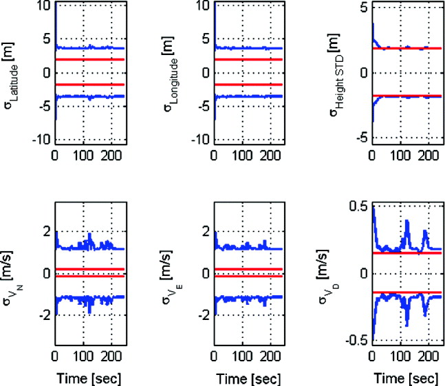
Figure 4. Position (LLH) and velocity (NED) components of the SA error model with position aiding. Red (straight lines) and blue lines represents the analytical and computed square root of the error covariance, respectively.
Evaluating the two aidings (position and position-and-velocity) for the SA model, it is can be seen that the addition of a velocity measurement enables an exact analytical prediction of the position components of the full 15 state model by only three parameters. Additionally, with both aiding types the analytical evaluation of the position and velocity components' height channel was similar to the full 15 state error model. This result is attributed to the fact that in the complete 15 state model the altitude channel performs like the SA model and that even use of the position aiding is sufficient for observing the altitude position and velocity states.
4.2. Aided Single Channel Error Model
We then evaluate the SC error model covariances. Covariance values are obtained by multiplying the SA analytical expressions for the square-root error covariance (Equation 18) by the correction factors which link the SA and SC models (Equation 26).
The correction factors are a function of the IMU, the aiding type (position or position-and-velocity), and the corresponding measurement noise level. As the IMU and aiding type can be assumed constant per a given system/scenario, we calculate the correction factors required for the specific IMU used in our field experiments as a function of the measurement noise level of the aiding sensor only.
We use the analytical SA (Equation 18) and the numerical aided SC (Equation 25) error model expressions and insert them into Equation (26) in order to obtain the correction factors. Figure 5 presents the correction factors for the SA error model with position-and-velocity aiding. They are plotted against the position-measurement-noise-level and for various velocity noise-level magnitudes. κ pos, which is equivalent to κ 11 in Equation (26), is the correction factor for the position error state and κ vel, which is equivalent to κ 22 in Equation (26), is the correction factor for the velocity error state.

Figure 5. SA error model correction factors for position and velocity measurements aiding
When the velocity aiding measurement noise is smaller than 0·1[m/s], the correction factors for both velocity and position are constant regardless of the amount of the position measurement noise. For higher velocity-measurement-noise values, both correction factors (position and velocity) converge to a constant value. That is, the correction factors can be considered constants regardless of the measurement noise and used incessantly with the SA error-model. This result was expected, as the filter gives lower weight to the measurement due to the amount of high measurement noise.
Figure 6 presents the position aiding correction factors as a function of the position measurement noise (computed in a similar fashion as for Figure 5). The velocity correction factors increase as the amount of measurement noise increases, while the position-correction-factor convergences to a constant value.

Figure 6. SA error model correction factors for position measurement aiding.
Following the computation of the correction factors, results for position and velocity aiding are presented in Figure 7. There, the position and velocity components of the square-root of the error covariance of the full 15-state model (which was calculated numerically) match exactly the SC analytical expressions for the square-root of the error covariance (Equation 26). This result was achieved, although the SC model has constant time dynamics and no coupling between its three orthogonal axes, in contrast to the full error model. Thus, we evaluate the results of the 15 error state aided INS model covariances by the semi-analytical expressions, making the numerical evaluation unnecessary.

Figure 7. Position (LLH) and velocity (NED) components of the SC error model with position and velocity aiding. Red (straight lines) and blue lines represents the analytical and computed square root of the error covariance, respectively.
The covariance values for the position aiding are presented in Figure 8. The position and velocity components of the square root of the error covariance of the full aided INS 15 error state model, which was calculated numerically, match exactly the SC semi-analytical expressions for the square-root of the error covariance. Thus, in the aided SC model, position measurement is sufficient to predict the position and velocity states despite of the fact that it has constant time dynamics and no coupling between its three orthogonal axes. Consequently, using only four variables of the INS quality, aiding value, and position and velocity correction factors, the covariances are evaluated.

Figure 8. Position (LLH) and velocity (NED) components of the SC error model with position aiding. Red (straight lines) and blue lines represents the analytical and computed square root of the error covariance, respectively.
Comparing the SC and SA aided models performance, shows that the SC model outperforms the SA model in predicting the full aided INS 15 error state model. This result was anticipated as the SC model is more accurate (because of the gyro and GM error-states) relative to the full-model rather than the SA model.
4.3. Application to Additional Trajectories
Application of the model to two additional trajectories with different characteristics shows the same prediction ability as with the analyzed trajectory. In this trajectory, the stationary vehicle accelerated to v=60[km/h], and then kept a velocity in the range of 60–80 [km/h]. The vehicle climbed along this trajectory ∼100 [m] in elevation. In the second trajectory, the stationary vehicle accelerated to 40[km/h], and then kept a velocity in the range of 40–60 [km/h].
In order to evaluate the proposed approach in different noise levels, we used for the second trajectory a noise-measurement-covariance which was five times bigger than the one used in trajectory 1, for both aidings and aided INS simplified error models. However, only the results for position and velocity aiding are presented here. As can be observed in Figures 9 and 10, for both SA and SC error models and both aiding types, a similar behavior to the first trajectory was obtained even with the different measurement noise level. That is, with the SA model and for both aiding types, the analytical evaluation of the height channel's position and velocity components was similar to the full 15 state error model, while the addition of velocity measurement enabled the complete position vector to be evaluated analytically. With the SC model, the position aiding was sufficient to predict the position and velocity states of the full 15 state model.

Figure 9. Position (LLH) and velocity (NED) components of the SA error model with position and velocity aiding. Red (straight lines) and blue lines represents the analytical and computed square root of the error covariance, respectively.

Figure 10. Position (LLH) and velocity (NED) components of the SC error model with position and velocity aiding. Red (straight lines) and blue lines represent the analytical and computed square root of the error covariance, respectively.
In order to evaluate the proposed approach in different noise levels, we used a one hundred times bigger process noise covariance for the GM states for the third trajectory. This was conducted for both aidings and both aided INS simplified error models. However only the results for position and velocity aiding are presented here, in Figures 11 and 12. As can be observed, the same performance as with the previous trajectories was obtained even with the different measurement noise level. With the SA model and for both aiding types the analytical evaluation of the height channel's position and velocity components was similar to the full error model, while the addition of velocity measurement enabled the whole position vector to be evaluated analytically. With the SC model, both aidings enabled prediction of the position and velocity states of the full 15 state model.

Figure 11. Position (LLH) and velocity (NED) components of the SA error model with position and velocity aiding. Red (straight lines) and blue lines represent the analytical and computed square root of the error covariance, respectively.

Figure 12. Position (LLH) and velocity (NED) components of the SC error model with position and velocity aiding. Red (straight lines) and blue lines represents the analytical and computed square root of the error covariance, respectively.
5. CONCLUSIONS
Land navigation with aided-INS is needed for a variety of applications. Evaluation of the navigation system in early stages of design and system implementation enables the navigation system performance to be examined relative to desired navigation accuracy. In this paper, an analytical insight into the parameters involved in the fusion between INS and an aiding sensor was gained. To that end, two simplified time-invariant aided-INS error models were employed. Using both models, closed form solutions in terms of the continuous steady-state estimation error covariance matrix were derived for evaluating the fusion performance. The closed form expressions of the simplified error models were compared to numerical results obtained from data collected in a field experiment, using the full 15 state error model. Results show that the derived closed form expressions managed to predict the error covariance behavior of the full error model. Even though these closed-from expressions are valid only for small fractions of the Schuler period, they bring insight into the effect of the various parameters involved in the fusion between the INS and an aiding sensor. They may help the navigation system designer to better evaluate and understand the connection of the parameters concerned in the fusion process. Future work will examine the effect of a Schuler feedback loop when evaluating the closed form expressions in medium and long term time periods. Additionally, since GPS is the main aiding sensor for the INS derivation of closed form expressions, the non-linear tightly coupled approach is another potential expansion of the presented models.
ANNEX A.THE CONTINUOUS KALMAN FILTER
We consider here the linear stochastic system:
where:
δx(t) is the error state vector.
δz(t) is the measurement residual.
w(t) and v(t) are the white Gaussian stochastic processes representing the system driving noise and the measurement noise, respectively.
δx(t 0) is a Gaussian random vector.
and:
![$$\eqalign{ & E[x_o ] = \overline x_o, E[w(t)] = 0,E[v(t)] = 0, \cr & E[w(t)w(t')^T ] = {\rm} Q\delta (t - t'),E[v(t)v(t')^T ] = R\delta (t - t'), \cr & E[w(t)v(t')^T ] = 0,E[w(t)x_o ^T ] = 0,E[v(t)x_o ^T ] = 0, \cr & E[(x_o - E(x_o ))(x_o - E(x_o )^T ] = P_o.} $$](https://static.cambridge.org/binary/version/id/urn:cambridge.org:id:binary:20151022042206496-0160:S0373463311000609_eqnA2.gif?pub-status=live)
All vectors and matrices are of appropriate dimensions. The Kalman filter (Zarchan et al., Reference Zarchan and Musoff2005) is:
The steady-state solution of the covariance, ![]() , is the solution of the ARE:
, is the solution of the ARE:
With the steady-state solution obtained from Equation (9), we have the explicit solution (Rusnak, Reference Rusnak1998):
![$$\eqalign{P(t) = & \ \overline P + \Phi (t,t_0 )\left( {\overline P_0 - \overline P} \right)\left[ {I + \int\limits_{t_0} ^t {\Phi ^T (\tau, t_0 )H^T R^{ - 1} H\Phi (\tau, t_0 )\left( {P_0 - \overline P} \right)d\tau}} \right]^{ - 1} \Phi ^T (t,t_0 ) \cr & {\rm \dot \Phi }(t,t_0 ) = \left[ {F - \overline PH^T R^{ - 1} H} \right]\Phi (t,t_0 )} $$](https://static.cambridge.org/binary/version/id/urn:cambridge.org:id:binary:20151022042206496-0160:S0373463311000609_eqnA7.gif?pub-status=live)
ANNEX B. RELATIONSHIP OF NONLINEAR ALGEBRAIC EQUATIONS IN TERMS OF THE NORMALIZED AND NON-NORMALIZED COVARIANCES ELEMENTS
The connection between the normalized and non-normalized steady-state error covariance terms is given by:
The connection between the normalized and non-normalized steady-state gain terms is given by: