3.2.1. The paddling dynamics

Here we examine the detailed swimming behaviour of A. aurita (h ₀/d ₀ = 0.3). For this, the active contraction of the subumbrellar jellyfish bell is initiated by applying a transient nodal force ${\boldsymbol{F}_b}$ (see (B9) and figure 1b) at the bell margin for non-dimensional time 0 < t ≤ t_c; while the subsequent passive expansion phase continues (see supplementary movie 2 available at https://doi.org/10.1017/jfm.2020.1069) following withdrawal of ${\boldsymbol{F}_b}$ during T − t_c and in which the stored elastic strain energy drives the bell expansion. A propulsion cycle herein is fixed at T = 2.0, and the chosen material elastic parameters are c_st = 18.5 and c_be = 0.03. The bell is thus driven forward for five cycles (t = 5T) using 50 ≤ Re ≤ 150 and $3 \le {\boldsymbol{F}_b} \le 27$. Moreover, the prey capture by a free swimming jellyfish is known to be better predictable for lower Re. While presenting the computed results, for non-dimensionalization, the fluid density ${\rho _0}$ is used as the characteristic density, bell diameter d ₀ as the characteristic length, and ${t_c}$ as the characteristic time. The other parameters are determined using following characteristic scales: $U = {d_0}/{t_c}$ for velocity, ${\rho _0}U/{d_0}$ for Eulerian momentum, ${\rho _0}{U^2}$ for Lagrangian momentum, ${\rho _0}{U^2}{d_0}$ for elastic stiffness coefficient and ${\rho _0}{U^2}d_0^3$ for bending coefficient (Park et al. Reference Park, Chang, Huang and Sung2014). The non-dimensional power P_m that is derived from the force ${\boldsymbol{F}_b}$ applied to the bell margin is therefore expressed as

(3.1)\begin{equation}{P_m} = \frac{{{F_b}(d - {d_{min}})/{t_c}}}{{\rho {d^5}/{T^3}}}.\end{equation}

Figure 3(a) shows the time history of distance ($y/{d_0}$) that is travelled by the jellyfish in five swimming cycles (0 ≤ t ≤ 10 = 5T) for the indicated three different magnitudes of the paddling body force ${\boldsymbol{F}_b}$. Moreover, figure 3(b–d) displays the periodic change of the subumbrellar bell volume $(V/{V_0})$, the non-dimensional power (P_m) and forward velocity $(v/U)$ of the bell centroid during the third to fifth cycles. The noted initial rapid decrease of the bell volume $(V/{V_0})$ in figure 3(b) in a cycle corresponds to fast forward swimming speed (figure 3d) that is generated during the contraction phase; while for higher ${\boldsymbol{F}_b}$ the bell volume is reduced at a faster rate that strengthens the forward body motion (figure 3a). Figure 3(c) reveals that power P_m increases quickly as active force ${\boldsymbol{F}_b}$ (see (B9)) is applied (for t ≤ t_c) to the bell. The subsequent rapid decrease of P_m is noteworthy, while ${\boldsymbol{F}_b}$ withdraws during relaxation. The power becomes briefly negative at the beginning of a recovery phase (figure 3c), as a jellyfish bell starts to expand freely by spending stored elastic energy in a contracted state (Tytell et al. Reference Tytell, Hsu, Williams, Cohen and Fauci2010). Additionally, power displays rapid/increased variation for higher ${\boldsymbol{F}_b}$.

Figure 3. Plotted for applied different body-force magnitudes (F_b) are: (a) the displacement (y/d ₀) of the bell during five cycles, (b) the periodic change of the bell volume (V/V ₀) during the third to fifth propulsive cycles, (c) dimensionless power (P_m) associated with the body force (F_b) at the bell edge, and (d) forward swimming velocity (v/U) during the third and fifth swimming cycles. Here Re = 100 and h ₀/d ₀ = 0.3.

Figure 4(a) shows that the periodic contraction and expansion of the jellyfish bell in power $({\boldsymbol{F}_b} \gt 0)$ and recovery $({\boldsymbol{F}_b} = 0)$ strokes generate distinct 3-D vortex rings of opposite rotational sense at the bell margin. These vortex rings act to entrain upstream fluid from above the bell into the subumbrellar cavity. The results are shown here for the fifth propulsive cycle (8 < t ≤ 10). A near-edge 3-D vortex ring 5*St.V. that is created by the forced power stroke (8 < t ≤ 9; figure 4a1–a8) is conventionally termed as the starting vortex (where 5* denotes the cycle number and St.V. is the abbreviation for starting vortex). Figure 4(a5–a8) shows that, as the bell expands freely in recovery stroke (9 < t ≤ 10), the stopping vortex ring 5*Sp.V. (figure 4a5–a8) is produced, which spins in the reverse direction. During growth, the stopping vortex partly intrudes into the bell cavity along with the sucked fluid at the bell margin. Note that the diameter of the starting vortex ring (5*St.V.) steadily decreases in a power stroke and that of a stopping vortex (5*Sp.V.) increases through a relaxation phase, while physical processes are controlled by ${\boldsymbol{F}_b}$ and material elasticity. Importantly, these vortex-rings-induced fluid motion keep supporting the forward motion (figure 3a) in a propulsive cycle. The appended velocity field (figure 4a1–a8) on the symmetry (xy) plane clearly exhibits dominance of the upward flow at the bell edge, in both power and recovery strokes. The dropped off starting (4*St.V.) and stopping (4*Sp.V.) vortex rings that temporarily dominate in the wake are created during the fourth propulsive cycle.

Figure 4. (a) Three-dimensional evolution of starting (5*St.V) and stopping (5*Sp.V) vortex rings at different times during the fifth propulsive cycle, for applied body force F_b = 12. Also shown here are the resulting velocity field on the streamwise symmetry plane, and temporarily dominating stopping (4*Sp.V) and starting (4*St.V) vortex rings in the near wake that are generated in the previous cycle. (b) The transient evolution of starting (5*St.V) and stopping (5*Sp.V) vortex rings in the fifth cycle, for the reduced body force F_b = 7. (c) Plots of out-of-plane vorticity (${\omega _z}$) contours at various times during the first, second, third and fifth swimming cycles (F_b = 7). In these vorticity (${\omega _z}$) plots, in the wake region of forward swimming jellyfish one can see progression of shedding of starting and stopping vortices. Here Re = 100 and h ₀/d ₀ = 0.3.

Figure 4(b) shows that, for a lower magnitude ${\boldsymbol{F}_b} = 7$ of the applied paddling force, the resultant weaker starting/stopping vortex rings evolve considerably closer to the bell edge, while the swimming speed (figure 3d) is greatly reduced. Notably, figures 4(b1) and 4(b5) display how exactly side-by-side evolving opposite-natured vortex ring pairs 4*Sp.V. and 4*St.V. or 5*Sp.V. and 5*St.V. actively entrain the outer fluid towards the bell edge. Figure 4(c) shows the out-of-plane vorticity $({\omega _z})$ at various times during the first, second, third and fifth cycles, exhibiting the near-field dominance of the respective starting and stopping vortices. The pressure contours presented in figure 5 show that lateral body motion helps the growth of significant low-pressure areas in the fluid surrounding the paddling bell. The animal uses this dominant low pressure to pull itself up through the surrounding water via suction-based propulsion, and it technically helps to drag floating nearby prey or copepods (see supplementary movie 1) to the bell margin via the stroke-by-stroke generated feeding current (see supplementary movie 2). The regions of high pressure, however, do form (Hoover et al. Reference Hoover, Griffith and Miller2017), especially in opposition to motion at the apex area (figure 5a1,a2) and during transient periods of lateral body motion, but these are clearly compensated (figure 3a) by virtue of suction-based upward momentum (figure 4a) that is produced by neighbouring fluid (Gemmell et al. Reference Gemmell, Colin, Costello and Dabiri2015).

Figure 5. (a1–a8) Isocontours of non-dimensional pressure at different instants during the fifth propulsive cycle. Near-surface transient pressure variations: during power stroke at (a1) t = 8.16, (a2) t = 8.4, (a3) t = 8.64 and (a4) t = 9; and during the recovery stroke at (a5) t = 9.28, (a6) t = 9.6, (a7) t = 8.88 and (a8) t = 10 ( = 5T). (b1) The marked horizontal lines are below the contracted bell, at the end of the fifth power stroke (t = 9). At these locations the variations of non-dimensional (b2) pressure, (b3) vertical velocity (v/U) and (b4) transverse velocity (u/U) are presented with respect to the (x) distance from the vertical axis. (c1) The marked horizontal lines below the expanded bell at the end of the fifth recovery stroke (t = 10), where variations of non-dimensional (b2) pressure, (b3) vertical velocity (v/U) and (b4) transverse velocity (u/U) are revealed with respect to the distance from the vertical axis. Here Re = 100 and h ₀/d ₀ = 0.3.

Variations of the non-dimensional pressure and vertical and transverse velocity along several horizontal slices that spread through the bell region as well as the near wake are revealed in figure 5(b1–c4) at the end of the fifth power and recovery strokes. Figure 5(b2) shows the formation of negative pressure in the bell, at the end of the contraction stroke. In contrast, at the end of the expansion stroke (figure 5c2), an elevated positive pressure develops at the cavity centre and relatively low-pressure areas are formed at the sides, suggesting the development of a pressure minimum at the core of vortex rings that dominate near the bell edge (figure 4). Moreover, the distribution of the vertical velocity (v/U) in figure 5(b3) reveals the existence of strong downward flow at different vertical locations, at the end of the power stroke; while positive velocity mostly persists near the bell boundary. These are in fact facilitated due to the ejection of the core fluid (like a jet) through the central part, and the entrainment of the surrounding fluid (see figure 4a3,a4) from the apex to the bell edge. At the end of the expansion phase, as evident from figure 5(c3), a strong positive vertical flow develops in the centre region owing to continued fluid entrainment (figure 4a5–a8) by the stopping vortex ring. Such velocity (v/U) gradually reduces at the edges and its direction is reversed at downstream locations. Figures 5(b4) and 5(c4) show that the transverse velocity (u/U) at each y station is reduced following pulsating motion as the vertical axis of symmetry is approached, while clear changes of sign occur at the two sides.

Figure 6(a1–a4) shows isocontours of non-dimensional vertical velocity (v/U) around the jellyfish during the fifth propulsive cycle, at t = 8.16, 9.0, 9.6 and 10.0; and figure 6(b1–b4) exhibits the corresponding radial velocity (u/U) contours. In the contraction phase, as a jellyfish moves forwards with larger speed, the stronger positive vertical and radial velocities (figures 6a1,a2 and 6b1,b2) develop at the top and around the bell (see figure 4a1–a4). The formation of negative and positive radial velocity regions (figure 6b1) at the bell edge or near wake are the results of mutual interaction of starting (5*St.V.) and stopping (4*Sp.V.) vortices in the propulsive power stroke, as evident from figure 4(a1). In the expansion phase, the presence of similar vertical and radial velocities (figure 6a3,a4,6b3,b4) in the vicinity of the bell are due to continued upward bell motion plus fluid entrainment into the bell cavity via the dynamics of the stopping vortex ring 5*Sp.V., as noted in figure 4(a6–a8). The observed negative vertical velocity areas in figure 6(a1–a4) around the bell margin are formed because of transfer plus rotation (figure 4a3,a4,a6–a8) of the surrounding outer fluid towards the bell edge; whereas the ejection of the inner fluid in the form of a jet and the interaction of the starting and stopping vortices continue to yield continuous columns of vertical flows away from the bell. The presence of positive/negative radial velocity regions at the bell edge or near wake, in figure 6(b3,b4), during the recovery phase are contributed by the interaction of 5*Sp.V. with the bell boundary (figure 4a6–a8).

Figure 6. Isocontour plots of non-dimensional (a1–a4) vertical velocity (v/U) and (b1–b4) radial velocity (u/U) around the paddling bell, at different instants during the fifth propulsive cycle. Here Re = 100 and h ₀/d ₀ = 0.3.

3.2.2. Variation of cost of transport (COT) and Strouhal frequency (St)

The COT is a convenient measure for determining energetic swimming performance. For a jellyfish the COT is defined as

(3.2)\begin{equation}COT = {E_i}/{d^{apex}},\end{equation}

where ${E_i} = \int_{{t_0}}^{{t_o} + T} {({F_b}(\textrm{d}r/\textrm{d}t))\,\textrm{d}t}$ is the required energy, ${d^{apex}}$ is the non-dimensional displacement of the bell apex in one propulsive cycle, $\textrm{d}r/\textrm{d}t$ is the rate of change in bell diameter and ${\boldsymbol{F}_b}$ is the applied paddling body force. The non-dimensional Strouhal number St is expressed as

(3.3)\begin{equation}St = d_{max}^{rad}/(Tv_{avg}^{apex}),\end{equation}

where $d_{max}^{rad}$ is the maximum radial displacement, T is the pulsating period and $v_{avg}^{apex}$ is the average apex velocity in a cycle.

Figures 7(a) and 7(b) show variations of COT and St ⁻¹ for two different bell fineness ratios 0.3 and 0.5, as functions of maximum paddling force ${\boldsymbol{F}_b}$, which helps to better comprehend morphological dependence. Moreover, the impact of resonant swimming on the variation of COT is revealed therein (its effect on prey capture is elaborated later). Figure 7(a) shows that COT increases rapidly for small ${\boldsymbol{F}_b}\,( \lt 4)$ that resemble cases of very low (see figure 3a,b) swimming speed (Gemmell et al. Reference Gemmell, Costello, Colin, Stewart, Dabiri, Tafti and Priya2013). Notably, for h ₀/d ₀ = 0.5 the optimum (minimum) COT occurs at a threshold ${\boldsymbol{F}_b} = 4$, and for h ₀/d ₀ = 0.3 such an optimum is reached at ${\boldsymbol{F}_b} = 7$; then COT slowly increases as ${\boldsymbol{F}_b}$ is increased. However, for applied higher ${\boldsymbol{F}_b}$ the increased drag (as drag is ~ v ²) due to the enhanced steady swimming speed plays a key role in increasing COT. The COT is found to be higher for the higher fineness ratio 0.5 (for ${\boldsymbol{F}_b} \ge 6$), signifying that an oblate-type body can be more economical. The larger stopping vortex that an oblate jellyfish creates (in a relaxation phase) and efficiently places under the enlarged bell plays an important role in reducing its COT, by virtue of passive energy recapture (Gemmell et al. Reference Gemmell, Costello, Colin, Stewart, Dabiri, Tafti and Priya2013). Additionally, figure 7(a) shows that COT is lowered via resonant swimming. Figure 7(b) shows that, despite fineness-ratio-dependent variation, St ⁻¹ increases rapidly at lower ${\boldsymbol{F}_b}\,( \le 12)$ and then slowly approaches the respective asymptotic limit for ${\boldsymbol{F}_b} \ge 25$, as peak propulsive efficiency is attained (Taylor, Nudds & Thomas Reference Taylor, Nudds and Thomas2003; Floryan, Buren & Smits Reference Floryan, Buren and Smits2018). Since the flapping frequency (1/T) of the bell is kept fixed here, St (equation (3.3)) varies as the ratio of flapping amplitude $(d_{max}^{rad})$ to forward distance that is travelled in a pulsing period. For higher ${\boldsymbol{F}_b}\,( \ge 25)$, St ⁻¹ approaches asymptotic limits, as noted in figure 7(b), which seems to imply that at this stage the distance that is travelled by a jellyfish varies nearly at the same rate as the flapping amplitude.

Figure 7. Plotted here are: (a) normalized cost of transport (COT/COT_ref) for non-resonant plus resonant swimming, and (b) the inverse Strouhal number (St ⁻¹), as functions of the magnitude of the applied paddling force (F_b). To reveal the morphological dependence of COT, the data for another fineness ratio (h ₀/d ₀ = 0.5) but with fixed body elasticity (i.e. c_st = 18.5 and c_be = 0.03) are added in panel (a), and the same reference COT_ref (i.e. for F_b = 12 and h ₀/d ₀ = 0.3) is used for normalization. Here Re = 100.

3.2.3 Circulation analysis

The circulation is an important issue (Colin et al. Reference Colin, Costello, Dabiri, Villanueva, Blottman, Gemmell and Priya2012) that plays a key role in medusan locomotion. Here we analyse the non-dimensional circulation $\varGamma$ , which is defined as the integral of vorticity over the area of a vortex ring on the symmetry plane, as follows:

(3.4)\begin{equation}\varGamma = \frac{T}{{d_0^2}}\int {{\omega _z}(x,y,0,t)\,\textrm{d}\kern0.7pt x\,\textrm{d}y} .\end{equation}

Figure 8 presents the computed variation of $\varGamma$ over five swimming cycles of A. aurita (h ₀/d ₀ = 0.3), for different magnitudes of the applied paddling force $7 \le {F_{\boldsymbol{b}}} \le 12$. It is noted that the circulations of starting (figure 8a) and stopping (figure 8b) vortex rings increase with the passing of time, as vortices gradually grow under time-varying ${\boldsymbol{F}_b}$ (figure 1c). Remarkably, despite a jellyfish producing (figure 3) greater acceleration during the power stroke, the resultant peak circulation by stopping vortex is about twofold higher than the peak circulation of the starting vortex, illustrating the important role of the stopping vortex in pulsating locomotion. Physically, during the relaxation phase, the outer fluid is continuously sucked into the expanding cavity (figure 4), whereas fluid from the top is being pushed down to the bell margin. This leads to increased circulation by the developed stopping vortex via passive energy recapture (Gemmell et al. Reference Gemmell, Costello, Colin, Stewart, Dabiri, Tafti and Priya2013). Moreover, as figure 8(a,b) shows, for increased paddling force ${\boldsymbol{F}_b}$, larger circulations are generated.

Figure 8. The non-dimensional circulation ($\varGamma$) of: (a) starting vortex ring, and (b) stopping vortex ring, in five swimming cycles, for the adopted different magnitude of the paddling force (F_b). Here Re = 100 and h ₀/d ₀ = 0.3.

3.3.1. The influence of prey inertia on predator–prey interaction

We now thoroughly examine prey interception and capture mechanisms based on the computed paddled swimming current, as a large taxonomy of zooplankton survives in this mode of hunting, and feeding-current-based nourishing is most effective (Humphries Reference Humphries2009) for various prey species. To start with, first the ideal case of infinitesimal prey is considered. The motion of plankton (of tiny mass) in this case coincides with that of ideal Lagrangian tracer particles. To demonstrate the prey interception mechanism, the essential forward-time and backward-time FTLE fields (Shadden et al. Reference Shadden, Dabiri and Marsden2006; Franco et al. Reference Franco, Pekarek, Peng and Dabiri2007; Green, Rowley & Haller Reference Green, Rowley and Haller2007) for a suspended layer of 4.9 × 10⁶ infinitesimal Lagrangian prey particles are computed using (3.7)–(3.10) and the flow field that is created (see figure 4a and supplementary movie 2) by paddling A. aurita (h ₀/d ₀ = 0.3, ${\boldsymbol{F}_b} = 12$).

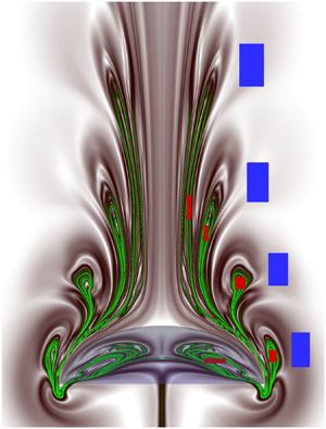
Figures 9(a) and 9(b) show contours of the forward-time and backward-time FTLE fields (at Re = 100) that are generated over a duration of five cycles (t = 5T). The related Eulerian velocity, vorticity and pressure fields are revealed in figures 4–6. Note in figure 9(a) the presence of four pairs of symmetrical FTLE lobes that are clearly detectable, as each pulsing cycle creates one such pair, while lobes formed in the fifth cycle appear weaker in this case. The corresponding high ridges (figure 9a), i.e. repelling pLCS are denoted by green contour lines. In figure 9(b), the ridges of the backward-time FTLE field (black contours) represent a sequence of attracting pLCS, and their outer boundary, which surrounds the developed five cavity-shaped multi-deck belly region (formed in five pulsing cycles) plus the area inside the bell, is defined here as the ‘capture boundary’. At a glance, figure 9 displays significantly distinct and physically/mathematically sound structures of prey interception loops and capture boundary (pLCS) compared with those reported earlier (Peng & Dabiri Reference Peng and Dabiri2009). These pLCS complement each other to transport floating prey from the frontal region into a jellyfish bell or suitable place in the near wake, or, alternatively, to preserve the recirculating prey that are already inside the capture surface (see supplementary movie 3).

Figure 9. Plotted here are the contours of FTLE fields and infinitesimal Lagrangian particles displaced by the paddling jellyfish (h ₀/d ₀ = 0.3). (a) The forward-time FTLE field, wherein the green-coloured high ridges reveal the Lagrangian coherent structures (LCS). Red and blue particles are placed inside and outside the upstream LCS lobes so as to track the fluid transport phenomenon and particle positions swept by the jellyfish motion. A greyscale colour map is also added for the reader's convenience. (b) The backward-time FTLE field and appended position of the displaced infinitesimal particles at t = 5T; the high ridges (LCS boundary), defined as the capture boundary, are denoted in dark black colour (as well as dashed green line, for clarity). Here Re = 100 and h ₀/d ₀ = 0.3.

To characterize which portions of the ambient fluid and locally present prey are targeted by a medusa/predator and which portion pass by without interacting, the red coloured Lagrangian tracer particles are placed inside pLCS lobes in figure 9(a) and blue-coloured particles outside. With such spatially distributed tracer particles, the simulation is re-run, as the paddling jellyfish swims across for five cycles (t = 5T), and the transient dynamics and positions of differently dragged particles are tracked. For clear distinction, in figure 9(b) we have appended the simulated final positions (at t = 5T) of coloured prey particles along with backward-time pLCS curves, confirming that the backward-time pLCS indeed form a capture boundary or capture surface. Figure 9(b) clearly shows that, through the paddled motion, all red particles are entrained within the pLCS boundary whereas clustered blue particles pass by without interacting. This shows that an infinitesimal plankton/copepod that is spotted inside mapped pLCS loops (figure 9a) can be captured for feeding, and those that remain outside have a good chance to escape. The supplementary movie 3 reveals the detailed stroke-by-stroke prey entrainment behaviour. However, although pLCS form a 3-D surface, the results are presented here on the streamwise symmetry plane, as conducting 3-D analysis often becomes costly and requires quite large CPU time plus RAM to track an enormous number of prey. However, the presented pLCS for ideal infinitesimal prey serves as a baseline to further examine the effects of prey inertia or escape force on a jellyfish's feeding performance, which are elaborated below.

We now study the effect of prey inertia, while momentarily ignoring the effect of escape force $({\boldsymbol{a}_E} = 0)$ in the modified Maxey–Riley equation (3.5). Notably, the term $- (R/2){\boldsymbol{a}_E}$ that appears in our (3.5) is missing in (2.1) of Peng & Dabiri (Reference Peng and Dabiri2009), where R (equation (3.6)) represents the combined influence of the mass of a prey and that of the displaced fluid, and the term can be obtained via a correct non-dimensionalization of the Maxey–Riley equation. To reveal a jellyfish's feeding on inertial copepods, first, using the flow field that is generated by paddled body motion and the dynamical system of equations (3.5)–(3.10), we compute the precise displacement pattern for the considered inertial prey particles with R = 2/3.

Figure 10 shows the resultant forward-time and backward-time FTLE fields, pLCS (dark coloured ridges) and positions of entrained (inner and outer) inertial prey particles of R = 2/3 (i.e. ${\rho _p} = {\rho _f}$; density of buoyant prey particles taken equal to the fluid density) due to the created feeding current by A. aurita (h ₀/d ₀ = 0.3) over five cycles. Note that the forward-time FTLE in figure 10(a) identifies four consistently formed (as in figure 9a) symmetrical pairs of fluid lobes or regions upstream; while lobes for the fifth cycle appear relatively weaker. To show that the extracted pLCS represent a realistic separation boundary for R = 2/3, the suspended red inertial particles are placed inside and blue particles outside the fluid lobes, as shown in figure 10(a), and then the simulation is re-run for five cycles, as the predator jellyfish swims across. Accordingly, the motion of differently dragged inertial prey particles is tracked, and for clarity their final positions (at t = 5T) are superimposed in figure 10(b) along with the backward-time pLCS. It reveals that the prey particles that stayed inside the FTLE lobes (in figure 10a) are mostly entrained within the multi-deck pLCS (figure 10b) boundary that surrounds five belly-shaped cavities formed in five pulsing cycles plus a part of the bell area; whereas those prey particles originated outside clearly escape. This demonstrates that the backward pLCS in figure 10(b) constitute the capture (or separation) boundary for inertial prey. Note that, for considered inertial preys (R = 2/3), the high ridges of backward FTLE (i.e. pLCS in figure 10b) appear relatively compressed at the top. Moreover, the positions of the dragged red particles in figure 10(b) suggest that some prey may have a small chance to escape by virtue of their inertia, particularly those stationed near the boundary of a forward-time FTLE/interception loop or the pLCS (figure 10a). Nevertheless, as figure 10(b) shows, the majority clearly fall inside the capture boundary.

Figure 10. Plotted for suspended inertial (R = 2/3) Lagrangian particles, the contours of FTLE fields and Lagrangian prey particles displaced by the paddling jellyfish at the end of the fifth pulsing cycle (t = 5T). (a) The forward-time FTLE field, wherein the green-coloured high ridges reveal the corresponding pLCS. Red and blue inertial particles are placed inside and outside the upstream pLCS lobes so as to track their swept positions by jellyfish motion. (b) The backward-time FTLE field plus appended position of the displaced inertial particles at t = 5T; the high ridges (pLCS) are denoted in dark black colour. Here Re = 100 and h ₀/d ₀ = 0.3.

To verify that the escape behaviour of some of the near-boundary inertial (figure 10b) prey is real or physical, we performed several simulations with varied prey density in a lattice (and escape force), and they exhibit the same repeat phenomenon. Note also that, for the infinitesimal case, each and every targeted red prey is dragged (figure 9a,b) inside the capture surface. This implies that capturing an infinitesimal prey can be easier for a medusa than capturing a finite-size prey (figure 10), i.e. that its inertia can help a prey to escape (Kiørboe Reference Kiørboe2011). The relative variations of the encounter loop, the capture surface and the success in prey capture for different cases are subsequently analysed. Prey capture for ${\rho _p} \gt {\rho _f}$ is not considered here, as that involves complex situations wherein prey swim along a deeper fluid layer than the predator.

3.3.2. Influence of prey escape force

The success in prey capture also depends on the evasive nature of a prey/copepod, as prey species often instantly accelerate to escape predation. The available experimental results (Kiørboe Reference Kiørboe2011) reveal that prey usually swim along a well-defined rather than a convoluted path, and the impulse of flow generated by a predator can be a warning signal for prey. We assume that the prey escape force ${\boldsymbol{a}_E}$ (3.5) has one of the following two different natures: (i) ${\boldsymbol{a}_E} = - {a_E}\boldsymbol{u}/|\boldsymbol{u}|$ or (ii) ${\boldsymbol{a}_E} = - {a_E}\boldsymbol{n} \times \boldsymbol{u}/|\boldsymbol{u}|$, where n is the unit normal vector to the plane of motion (Peng & Dabiri Reference Peng and Dabiri2009). In case (i), the escape force acts in the direction opposite to the local flow; while for case (ii), the escape force has direction normal to the local velocity and is directed away from a predator. Herein two different non-dimensional ${a_E} = 0.5$ and 0.25 are explored for the above two escape models, which fall within the reported (Strickler Reference Strickler1975) momentary escape acceleration limit up to 12 m s⁻² of a tiny prey.

For evasive prey (R = 2/3, ${a_E} = 0.5$) that attempt to escape opposite to local flow (i.e. case (i) above), figure 11 shows the forward-time (figure 11a1) and backward-time (figure 11a2) FTLE fields and their high ridges (pLCS), computed over five cycles. Among the five detected pairs of upstream prey interception zones (i.e. dark green FTLE lobes) in figure 11(a1), note in this case that, for opposite escaping prey, the lobes that are formed in the third and fourth cycles are decisively larger/longer than those for non-escaping inertial prey (figure 10a). The noted development of larger loops in figure 11(a1) at later cycles particularly reverses several reported conclusions in Peng & Dabiri (Reference Peng and Dabiri2009) based on the results in their figures 1 and 2 and table 1, which are obtained for nearly two swimming cycles, when the effects of swimming current and the considered opposite escape acceleration/response of prey are yet to become effective. Accordingly, the initial lobe sizes became smaller. Note also the natural open shape of forward-time pLCS in figure 11(a1), at the front side of a predator. Figure 11(a2) shows that the topmost boundary of the backward-time pLCS or capture boundary in this case has moved considerably inside the jellyfish bell with respect to infinitesimal (figure 9b) and non-escaping inertial (figure 10b) prey, signifying its local shrinkage for opposite escaping prey. The precise variation of the prey capture region for the investigated cases is summarized later.

Figure 11. Plotted for oppositely escaping prey with two different escape accelerations, ${a_E}$ = 0.5 and ${a_E}$ = 0.25, the contours of FTLE fields (pLCS) and displaced prey particles via the paddling jellyfish motion. (a1) The forward-time FTLE field, where green-coloured high ridges reveal pLCS computed at t = 5T, for ${a_E}$ = 0.5. The red and blue coloured opposite escaping prey particles are initially located inside and outside the upstream pLCS lobes, and their swept positions are tracked as the jellyfish paddles forwards. (a2) The backward-time FTLE field plus appended position of displaced opposite escaping (${a_E}$ = 0.5) prey at t = 5T; the pLCS boundaries are denoted in dark black colour. (b1, b2) Displayed results that are computed for a reduced prey escape acceleration, ${a_E}$ = 0.25. Here Re = 100 and h ₀/d ₀ = 0.3.

To demonstrate the capture of such evasive prey in a consistent manner, the red prey particles are placed inside pLCS lobes in figure 11(a1) and blue prey particles outside; all prey try to escape oppositely. With such spatial prey positions, the simulation is re-run, as the paddling jellyfish moves forwards for five cycles (t = 5T), and the swept/transient prey (via feeding current) locations are tracked. For clarity, the final position of swept prey particles (due to created feeding current) are superimposed in figure 11(a2) along with backward-time pLCS. This displays that the majority of the targeted red prey that originated within forward-time FTLE loops (in figure 11a1) are in fact contained within the capture area (high ridges of backward-time pLCS), while some apparently escape using the executed instantaneous acceleration. Figure 11(a2) also shows that all blue-coloured prey (which originated outside the loops) effectively move out of the capture boundary. Additionally, at a reduced prey escape acceleration ${a_E} = 0.25$, the presented Lagrangian analysis in figure 11(b1,b2) shows a consistent capture behaviour for the oppositely escaping preys (i.e. for case (i)).

For prey that attempts to escape normal to the local flow (${\boldsymbol{a}_E} = - {a_E}\boldsymbol{n} \times \boldsymbol{u}/|\boldsymbol{u}|$, i.e. case (ii) above), figures 12(a1) and 12(a2) show forward-time and backward-time FTLE fields plus pLCS at ${a_E} = 0.5$, along with the appended swept prey position (at t = 5T). Figures 12(b1) and 12(b2) exhibit the corresponding results at a lower ${a_E} = 0.25$. Note that, at a fixed ${a_E} = 0.5$, for normally escaping prey, the interception zones shift significantly closer to the predator body and loop sizes became relatively larger in the first two cycles but decisively smaller in the third and fourth cycles, compared to oppositely escaping preys. The clear distinction of such results with Peng & Dabiri (Reference Peng and Dabiri2009) is noteworthy, as those are obtained using data from small-time swimming (when the surrounding flow has not adequately developed). Moreover, a close look at figures 12(a1,b1) and 13(a3) reveals, for the reduced normal escape acceleration ${a_E} = 0.25$, that the resultant loop sizes become larger. The shrinking of the loop sizes at a higher normal escape force is in fact expected in a natural predator–prey environment.

Figure 12. For normally escaping prey with two different escape accelerations, ${a_E}$ = 0.5 and ${a_E}$ = 0.25, shown here are contours of FTLE fields (pLCS) and (escaping) prey particles displaced by the paddled jellyfish motion. (a1) The forward-time FTLE field, where green-coloured high ridges reveal corresponding pLCS computed at t = 5T; ${a_E}$ = 0.5. The red and blue coloured normally escaping preys are initially located inside and outside the upstream pLCS lobes, and their swept positions are tracked as the jellyfish swims forwards. (a2) Backward-time FTLE field plus appended position of normally escaping (${a_E}$ = 0.5) prey at t = 5T; the pLCS boundaries are denoted in dark black colour. (b1, b2) Displayed results that are computed for a reduced normal escape acceleration, ${a_E}$ = 0.25. Here Re = 100 and h ₀/d ₀ = 0.3.

Figure 13. The variation of forward-time pLCS (encounter loops) for different types of prey. (a1) Curves are: solid red lines with circles, ideal infinitesimal (Inf.) prey; solid black lines, inertial prey with no escape force (R = 2/3, NESCF, ${a_E}$ = 0); dashed blue lines, inertial prey with opposite escape force (OESCF, ${a_E}$ = 0.25); dotted green lines, inertial preys with normal escape force (NRESCF, ${a_E}$ = 0.25). Panel (a2) shows the influence of increased opposite escape force. Curves are: solid black lines, inertial prey with no escape force (R = 2/3, NESCF, ${a_E}$ = 0); dashed blue lines, inertial prey with opposite escape force ${a_E}$ = 0.25 (OESCF, ${a_E}$ = 0.25); dotted green lines, inertial prey with a higher opposite escape force ${a_E}$ = 0.5 (OESCF, ${a_E}$ = 0.5). Panel (a3) shows the influence of increased normal escape force (NRESCF). The notation is the same as above. Here Re = 100 and F_b = 12. Panel (a4) shows the influences of increased paddling force (F_b) and Reynolds number (Re). Panels (b1–b4) show the 3-D structure of prey encounter loops (forward-time pLCS) for: (b1) ideal infinitesimal prey; (b2) inertial prey with no escape force (R = 2/3, NESCF,${a_E}$ = 0); (b3) inertial prey with opposite escape force (R = 2/3, OESCF, ${a_E}$ = 0.5); and (b4) inertial prey with normal escape force (R = 2/3, NRESCF, ${a_E}$ = 0.5). Here h ₀/d ₀ = 0.3.

Figures 13(a1)–13(a4) present a detailed comparison of prey interception loops on the streamwise swimming plane for the above examined different cases of varied prey inertia and escape acceleration, whereas their 3-D structures are revealed in figures 13(b1)–13(b4). Supplementary movie 4 displays transient transformation of the forward-time pLCS into backward-time pLCS as the direction of time integration is reversed, while supplementary movie 3 clearly exhibits that prey that originates within forward-time pLCS lobes is basically captured by a jellyfish (either brought to the bell cavity or preserved within the multi-deck capture boundary that is demarcated by the backward-time pLCS). Importantly, the capture boundary that is defined in this study using the backward-time pLCS remains consistent all along, and the supplied movies provide a realistic view for stroke-by-stroke prey capture. On the other hand, the previously postulated capture area (Peng & Dabiri Reference Peng and Dabiri2009) was defined without computing the required backward-time pLCS. Moreover, it is clear from figure 13(a1–a3) that the FTLE loops that formed in later cycles predict decisively opposite (enhanced/weakened) capture performance (as the feeding current of a predator amply spreads) with respect to loops that formed in the first or second cycles. This suggests that any analysis based on short-time data can lead to factually erroneous estimation of inertia/escape-force-dependent prey capture performance. Notably, from the physical point of view, the forward-time FTLE loops (prey interception loops) for the initial two swimming cycles are formed mostly along the (left/right) sides of a predator, where local flow remains downward-directed. Accordingly, the loop sizes (in two cycles) exhibit a decreasing trend for inertial (non-escaping) and escaping prey with respect to an ideal infinitesimal prey. As figure 13(a1–a3) displays, this is in contrast to the FTLE loops (pLCS) for subsequent cycles formed at an adjacent frontal/downstream region of a forward-swimming jellyfish where local velocity is reversed/upward-directed. Therefore, opposite escaping prey $({\boldsymbol{a}_E} = - {a_E}\boldsymbol{u}/|\boldsymbol{u}|)$ that swim at the frontal region of the bell apex mistakenly move close to the predator/jellyfish instead of actually evading. This, in fact, helps predation plus capture. Consequently, for opposite escaping prey, the interception/target loops/fingers that are formed in the third and fourth cycles (and stretch along the front side) become longer/larger (see figure 13a1–a3) compared to those for stationary (non-escaping) prey; whereas the loops created by the first and second cycles often reveal the opposite trend. The decisively important longer loops for the third and fourth cycles are absent in Peng & Dabiri (Reference Peng and Dabiri2009), which, when taken into account, actually reverses the analysis in their tables 1 and 2, as evidenced below herein (figures 20 and 21, and table 3). In addition, figure 13(a4) shows that increased Re results in growth of larger-sized FTLE loops or prey encounter loops.

Note that for intercepted normally escaping prey at a higher a_E = 0.5, as figure 13(a3) presents, in the fourth and third swimming cycles the smaller-sized FTLE loops are generated compared to those at a_E = 0.25, while loops that formed in the first cycle reveal the visibly reverse trend. Figure 13(a4) shows that the interception loop areas significantly increase at a higher F_b. This signifies that, for self-propelled zooplankton, the magnitude of the propulsive force can have a profound effect on the feeding performance (Kiørboe et al. Reference Kiørboe, Jiang, Goncalves, Hielsen and Wadhwa2014).

3.3.3. Fluid-signal-based escape strategy and performance

For above considered cases, the prey escape response is initiated as soon as the disturbance that is created by a predator reaches a prey. However, in reality, the startle response for a copepod/prey attempting to escape predation is often initiated once an appreciable fluid signal/deformation that is generated by the predator becomes a threat. Motile prey often distinguish such fluid disturbances (Kiørboe et al. Reference Kiørboe, Saiz and Visser1999) and intend to escape a feeding current. In general, the escape signal can be a disturbance in velocity or acceleration, but the most recognized signal is the local shear rate. Accordingly, we assume here that a prey starts escaping as the local shear rate reaches a threshold value, which is then continued even if the shear rate drops later.

Figure 14(a) shows the threshold $({\tau _{th}} = 1)$ shear-dependent variations of prey interception loops (pLCS) for opposite escaping $({\boldsymbol{a}_E} = - {a_E}\boldsymbol{u}/|\boldsymbol{u}|)$ prey, relative to those that escape naturally $({\tau _{th}} = 0)$. The pLCS are computed over five swimming cycles of the predator. Note that, for the initial two cycles, the loop sizes decrease as the threshold value for perception decreases, a trend that is consistent with the measurements reported by Peng & Dabiri (Reference Peng and Dabiri2009) in their figure 3. In contrast, as figure 14(a) displays, the loops that are created in the third and fourth cycles appear significantly larger than the loops formed in the first and second cycles, and these later loops in fact play a decisively important role in interception/capture of the oppositely escaping prey. Furthermore, the characteristic variation of loops that formed in the third and fourth cycles is very much reversed for prey that escape naturally $({\tau _{th}} = 0)$, with respect to those escape at threshold shear $({\tau _{th}} = 1)$. This is because an oppositely escaping prey that stayed in the adjacent frontal region mistakenly moves towards the predator jellyfish (due to prevailing locally upward flow) instead of actually evading. The previously reported results (table 2 in Peng & Dabiri Reference Peng and Dabiri2009) lack contributions from such decisively larger loops (formed in the third and fourth cycles), plus the influence of the missing term $- (R/2){\boldsymbol{a}_E}$. However, the interception loops in the fifth cycle appear relatively unclear (due to weaker local flow) as they formed far from the swimming body, and those loops are thus omitted. Figure 14(b) shows the threshold shear-dependent variations of FTLE loops for normally escaping $({\boldsymbol{a}_E} = - {a_E}\boldsymbol{n} \times \boldsymbol{u}/|\boldsymbol{u}|)$ prey. In this case, except for the first cycle, the loop sizes increase as the threshold value for perception is increased. Furthermore, as figure 14(b) shows, despite a consistent open shape at the front side, for normally escaping prey, the FTLE loops or pLCS converge noticeably close to the vertical symmetry line, and their sizes decrease with respect to opposite escaping preys (figure 14a).

Figure 14. Threshold shear-dependent variation of pLCS for oppositely and normally escaping prey in five swimming cycles. Forward-time pLCS/FTLE loop areas and their locations reveal the relative variation of the prey interception regions with respect to the jellyfish. The dotted lines are ${\tau _{th}} = 0$ (constant escape response); and the dashed lines are ${\tau _{th}} = 1$ (escape response applied at a threshold shear). (a) Opposite escaping prey; and (b) normally escaping prey. Abbreviations used here are: OESCF, opposite escape force; OESCF-Th, opposite escape force applied at threshold ${\tau _{th}} = 1$; NRESCF, normal escape force; NRESCF-Th, normal escape force applied at threshold ${\tau _{th}} = 1$. Here Re = 100 and h ₀/d ₀ = 0.3.

3.3.4. Influence of paddling force

We now examine the paddled force-dependent, ${\boldsymbol{F}_b}$, variations (Nielsen et al. Reference Nielsen, Asadzadeh, Dolger, Walther, Kiørboe and Andersen2017) of prey interception and capture, and infinitesimal prey are considered for the analysis. Figures 15(a1) and 15(a2) show forward-time and backward-time FTLE fields, pLCS and appended final prey positions, for ${\boldsymbol{F}_b} = 7$; and figure 15(b1,b2) reveals such results for ${\boldsymbol{F}_b} = 17$. First, the appended final positions (at t = 5T) of the displaced prey particles in figures 15(a2) and 15(b2) that originated both within the forward-time FTLE lobes (denoted in red in figure 15a1,b1) and outside (marked in blue) following five cycles of the created feeding current (by A. aurita, h ₀/d ₀ = 0.3) exhibit that the red prey are contained in a capture zone (pLCS boundary) whereas blue particles stay out/escape. Second, a comparison of figure 9(a,b) with figures 15(a1,a2) and 15(b1,b2) clearly reveals that the target loops and prey capture zones become bigger/more elongated as the magnitude of the paddling force (${\boldsymbol{F}_b}$, (B9)) is increased, signifying the prospect of an improved feeding efficiency (figure 20). Notably, despite ${\boldsymbol{F}_b}$-sensitive variations, all infinitesimal red prey that originated within forward-time FLTE loops (e.g. figures 15a1,b1 and 9a) are entrained into the respective capture boundary (backward-time pLCS; figures 15a2,b2 and 9b) while those that stayed outside clearly escape. Therefore, the observations from figure 10(b) strongly suggest that their inertia can help some prey to escape.

Figure 15. The impact of varied paddling force (F_b) on prey capture. Plotted for infinitesimal prey and applied to two different paddling forces, F_b = 7 and F_b = 17, the contours of FTLE fields (pLCS) and displacement of prey particles due to the paddling jellyfish motion. (a1) The forward-time FTLE field, where green-coloured high ridges reveal Lagrangian coherent structures (pLCS) computed at t = 5T, for F_b = 7. The red- and blue-coloured prey are initially located inside and outside the upstream pLCS lobes, and their swept positions are tracked, as the jellyfish moves forwards. (a2) The corresponding backward-time FTLE field plus appended position of prey at t = 5T; the pLCS boundaries are denoted in dark black colour. (b1, b2) Displayed results that are computed for increased paddling force F_b = 17. Here Re = 100 and h ₀/d ₀ = 0.3.

3.3.5. Effect of Reynolds number

Figure 16 presents the Lagrangian analyses for varied Re. For Re = 50, figure 16(a1) shows the forward-time FTLE plus pLCS (dark green high ridges), and figure 16(a2) reveals the backward-time FTLE/pLCS (black high ridges) that are computed for five swimming cycles. Figures 16(b1) and 16(b2) display such simulated results at Re = 150. Figures 16(a1) and 16(b1) show that the sizes of FTLE lobes (target zones) increase for increased Re, signifying the possibility of improved prey encounter and capture (e.g. figures 13a4, 17 and 20). For essential details, the pink-coloured individual infinitesimal prey particles are placed within the forward-time FTLE lobes (figure 16a1,b1) and blue prey particles are placed nearby/outside. Computations are thus performed for five cycles, as the predator/jellyfish swims forwards. In figures 16(a2) and 16(b2) the appended swept positions of the prey particles (at t = 5T) confirm that prey that originated inside the forward-time FTLE lobe (figure 16a1,b1) are entrained within the respective pLCS boundary (figure 16a2,b2), while those stayed outside visibly escape. It is noteworthy that the prey that stayed inside FTLE loops (figure 16a1,b1) created in the third and fourth cycles are also effectively entrained within the bell region (see figure 16a2,b2), and the capture area is clearly increased at a higher Re.

Figure 16. The impact of increased Reynolds number (Re). Plotted for infinitesimal prey and for two different Reynolds numbers, Re = 50 and Re = 150, the contours of FTLE fields (pLCS) and displaced prey particles due to the jellyfish motion. (a1) The forward-time FTLE field, where green-coloured high ridges reveal Lagrangian coherent structures (pLCS) computed for t = 5T, using Re = 50. The pink- and blue-coloured prey particles are initially located inside and outside the upstream pLCS lobes, and their swept positions are tracked as the jellyfish paddles forwards. (a2) The corresponding backward-time FTLE field plus appended position of prey at t = 5T; the pLCS boundaries are denoted in dark black colour. (b1, b2) Displayed results that are computed for the increased Re = 150. Here h ₀/d ₀ = 0.3.

Figure 17. Plotted here are the prey capture areas (defined by outer high ridges of backward-time pLCS) on the streamwise (z = 0) swimming plane, for floating: (a1) infinitesimal prey, Re = 100 and F_b = 12; (a2) infinitesimal prey, at Re = 50, F_b = 12; (a3) infinitesimal prey, at F_b = 17, Re = 100; (a4) infinitesimal prey, at F_b = 7, Re = 100; (a5) inertial prey with no escape force (R = 2/3, NESCF, ${a_E}$ = 0), Re = 100 and F_b = 12; (a6) inertial prey with opposite escape force (R = 2/3, OESCF, ${a_E}$ = 0.5), Re = 100 and F_b = 12; and (a7) inertial prey with normal escape force (R = 2/3, NRESCF, ${a_E}$ = 0.5), Re = 100 and F_b = 12. (b1–b7) The exhibited 3-D structures of corresponding prey capture surfaces. Here h ₀/d ₀ = 0.3.

To exhibit the relative variation of capture area/volume for infinitesimal, inertial, opposite and normally escaping prey, and for varied paddled force (F_b) and Re, these results are first summarized in figure 17(a1–a7) for the streamwise swimming plane. Figures 17(a1), 17(a5) and 17(a6) show that the capture area is reduced for inertial and oppositely escaping prey, with respect to infinitesimal prey, whereas the capture area (see figure 17a1–a4) increases as paddled body force (F_b) or Reynolds number (Re) increases. Moreover, for improved clarity, in figure 17(b1–b7), the multi-decked 3-D structures of the prey capture surfaces for the various cases examined are presented for five paddled cycles.

3.3.6. Prey capture at resonant frequency

Past findings (Alexander & Bennet-Clark Reference Alexander and Bennet-Clark1977; Tytell et al. Reference Tytell, Hsu, Williams, Cohen and Fauci2010) suggest that, for faster motion, an aquatic swimmer often tunes muscle contraction appropriately with respect to surrounding fluid forces, which results in optimized body dynamics and maximization of peak acceleration. Accordingly, the resonant driving of the elastic bell is detected (Hoover et al. Reference Hoover, Porras and Miller2019) to maximize the forward swimming speed of a jellyfish relative to lower frequencies. To the authors’ knowledge, there exists virtually no study that examines or quantifies the impact of resonant swimming by a jellyfish on its prey capturing capability. To address this point, the present 3-D MRT-LB-IB model is utilized to explore the effect of resonant driving on prey encounter and capture.

To detect the natural frequency, for a selected paddling force (F_b), the bell diameter (d/d ₀) is initially allowed to contract to 90 % of its original length and then F_b is released indefinitely. This allows the body to oscillate freely in the fluid. As figure 18(a) shows, the periods of free vibration for the two different bells (of diameter d/d ₀) examined are $T_o^\ast = 3.07{t_c}$ at h ₀/d ₀ = 0.3 and $T_p^\ast = 3.79{t_c}$ at h ₀/d ₀ = 0.5, which correspond to the period of time beginning from the point after a bell has freely expanded from the starting contracted state to its next subsequent expansion state. The computed displacement of the apex of a jellyfish (h ₀/d ₀ = 0.3) bell as a function of $t/T_o^\ast $ is presented in figure 18(b) for three different normalized periods $T^{\prime} = T/T_o^\ast $, and it reveals that a bell with a shorter $T^{\prime}$ accelerates more quickly than one with a longer $T^{\prime}$. Note that, among all (smaller/larger) swimming periods $T^{\prime}$, the bell moves farthest (even after 15 cycles have elapsed) when it is driven at resonance $(T^{\prime} = 1)$. On the other hand, figure 7(a) shows that, when a jellyfish (h ₀/d ₀ = 0.3) swims at resonant frequency, its COT is clearly reduced over a range of applied paddling force (F_b). Now we focus on the issue of prey capture or hunting, as a jellyfish drives at resonant frequency.

Figure 18. (a) The oscillations of two bell diameters (d/d ₀) with h ₀/d ₀ = 0.3 and h ₀/d ₀ = 0.5 during free vibration study as functions of time (t/t_c). The paddling force F_b is applied until the bell diameter is reduced to 90 % and then released, allowing the bell to oscillate at its natural frequency of free vibration. Here Re = 100. (b) The plot reveals the displacement of a bell apex (h ₀/d ₀ = 0.3) as a function of time $t^{\prime}$ ( = $t/T_o^\ast $, where $T_o^\ast $ is the period of free vibration of the oblate-shaped bell) for three different normalized periods $T^{\prime}$ ( = T/$T_o^\ast $) = 0.65, 1.0 and 1.5.

Accordingly, figure 19 presents simulated prey interception loops (forward-time pLCS in five cycles) for three different selected driving periods of a jellyfish bell (h ₀/d ₀ = 0.3), which are: below the resonant driving $(T^{\prime} = 0.65)$, coincident with the resonant driving $(T^{\prime} = 1)$, and exceeding the resonant driving $(T^{\prime} = 1.5)$. As figure 19 shows, for all $T^{\prime}$, the distance of developed pLCS lobes from a bell increases in successive cycles, while the impact of the resonant driving (dotted loops) is clearly effective beyond the first swimming cycle. Notably, figure 19 also shows that, for increased period $(T^{\prime})$ of propulsive driving, the sizes of the interception loops increase with each passing cycle. Similarly, the size of the backward-time pLCS also become longer and larger with increased driving period $(T^{\prime} \gt 1)$ beyond the resonant driving; however, those results are omitted here for the sake of brevity. The issue of resonant-driving-affected prey clearance is analysed next.

Figure 19. This shows the effect of the resonant swimming on the formation of prey encounter loops (forward-time pLCS), for an oblate jellyfish (h ₀/d ₀ = 0.3) that intercepts floating infinitesimal prey. The three different selected driving periods are subresonant driving ($T^{\prime}$ = 0.65), resonant driving ($T^{\prime}$ = 1) and above-resonant driving ($T^{\prime}$ = 1.5). Here Re = 100 and F_b = 12.

3.3.7. Encounter rate

As elaborated above, medusae inhabiting the oceanic environment create a sequence of vortex rings via their repeatedly pulsed bell (Kiørboe et al. Reference Kiørboe, Saiz and Visser1999; Dabiri et al. Reference Dabiri, Colin, Costello and Gharib2005; Gemmell et al. Reference Gemmell, Colin, Costello and Dabiri2015), which in turn generates the necessary feeding current that transports/entrains (supplementary movies 1 and 5) nearby tiny copepods/prey into the belly or suitably pushes prey through the tentacles for filtering/ingestion. Many metazoans use filter feeding to catch bacteria-sized prey (Acuna, Lopez-Urrutia & Colin Reference Acuna, Lopez-Urrutia and Colin2011; Nielsen et al. Reference Nielsen, Asadzadeh, Dolger, Walther, Kiørboe and Andersen2017). However, the body shapes of prey and predator, the feeding current velocity and the ability of prey to escape can significantly impact prey filtering and capture (Kiørboe et al. Reference Kiørboe, Saiz and Visser1999). While computation of the prey encounter rate (E = Av, with A the area of filter and v the plankton velocity) is quite difficult due to the dynamic nature of the trailing tentacles plus the complexity of fluid/plankton velocity in the near wake, nevertheless, here we estimate the clearance rate CR (Nielsen et al. Reference Nielsen, Asadzadeh, Dolger, Walther, Kiørboe and Andersen2017) as the net volume flow of plankton/prey per swimming cycle per unit downstream distance d ₀ that extends below the bell margin, i.e.

(3.11)\begin{equation}CR = \tfrac{1}{3}\int_{3{d_0}} {\boldsymbol{v}\boldsymbol{\cdot}\boldsymbol{n}\,\textrm{d}l} .\end{equation}

Figure 20(a) shows the variation of the normalized clearance rate, CR/CR_ref, as a function of F_b, for ideal infinitesimal prey in the fifth cycle, which is examined for two jellyfish bell shapes of fineness ratio 0.3 and 0.5 and for resonant swimming. These relate to thrust production by jellyfish that drives the feeding current. It should be noted that, for an infinitesimal plankton, its velocity v is the same as the local fluid velocity (e.g. Nielsen et al. Reference Nielsen, Asadzadeh, Dolger, Walther, Kiørboe and Andersen2017), whereas v varies for inertial/escaping plankton. Figure 20(a) shows that, at a fixed Re = 100, the clearance rates CR/CR_ref for the said two jellyfish species increase significantly faster over 1 < F_b ≤ 11 and then gradually approach respective saturating states. However, for F_b ≥ 6, the CR/CR_ref value for the oblate species (h ₀/d ₀ = 0.3) far exceeds that of a prolate-type (h ₀/d ₀ = 0.5) predator, revealing a higher prey clearance capability for the former. This justifies why an oblate medusa is called a filter feeder, whereas a prolate one is a typical ambush predator (Kiørboe Reference Kiørboe2011). Significantly, for the created symmetric flow (figures 4 and 5) that surrounds a jellyfish, the presented normalized CR/CR_ref helps quantification of the required optimal propulsive force.

Figure 20. Plotted here are normalized: (a) clearance rate (CR/CR_ref), and (b) cost of preying (COP/COP_ref; (3.12)) in the fifth cycle, as a function of the magnitude of the applied paddling force (F_b). To reveal morphological dependence, data for another fineness ratio (h ₀/d ₀ = 0.5) are added to these two plots, and the same reference conditions (F_b = 12 and h ₀/d ₀ = 0.3) are used for normalization. The results for resonant (Res.) driving are also supplied that reveal the effects of the resonant swimming. For A. aurita (h ₀/d ₀ = 0.3) computed variations of: (c) clearance rate (CR/CR_ref) and (d) cost of preying (COP/COP_ref) in the fifth cycle while encountering the ideal infinitesimal (Inf.), inertial (R = 2/3, NESCF, ${a_E}$ = 0), opposite escaping (R = 2/3, OESCF, ${a_E}$ = 0.5), opposite escaping at threshold shear (R = 2/3, OESCF-Th, ${a_E}$ = 0.5), normally escaping (R = 2/3, NRESCF, ${a_E}$ = 0.5), and normally escaping prey at threshold shear (R = 2/3, NRESCF-Th, ${a_E}$ = 0.5). Here Re = 100.

Moreover, the results presented in figure 20(a) imply that the resonant swimming by a jellyfish/predator is inappropriate for the purpose of feeding, as CR/CR_ref is clearly reduced for both fineness ratios 0.3 and 0.5. However, the increased Re effectively increases CR/CR_ref for A. aurita (h ₀/d ₀ = 0.3). For an explicit quantitative measure, table 2 shows that for A. aurita (h ₀/d ₀ = 0.3) the average clearance rate $\overline {CR/C{R_{ref}}} $ over a range of applied paddling force 2 ≤ F_b ≤ 24 is reduced to 59 % when the jellyfish drives at natural frequency, whereas increased Re from 100 to 150 improved $\overline {CR/C{R_{ref}}} $ to 123 % of the corresponding non-resonant driving. On the other hand, as the fineness ratio is increased to 0.5 (i.e. for a prolate-type species, and at fixed Re = 100), the $\overline {CR/C{R_{ref}}} $ value reduced to 49 % of that at h ₀/d ₀ = 0.3. Additionally, when the prolate-type body drives at resonance, its clearance rate is further reduced to 86 % of the corresponding non-resonant case.

Table 2. In the fifth swimming cycle, the average clearance rate $\overline {CR/C{R_{ref}}} $ of ideal infinitesimal (Inf.) prey, over a range of applied paddling forces, 2 ≤ F_b ≤ 24. Here Res. denotes respective cases of resonant driving.

To determine an optimal feeding strategy, depending on the required input energy ${E_i}$ (equation (3.2)), the cost of preying for a feeding-current-generating predator is defined herein as

(3.12)\begin{equation}COP = \frac{{{E_i}}}{{CR}}.\end{equation}

Figure 20(b) shows the variation of the normalized COP/COP_ref for two different jellyfish shapes, over a range of applied paddling force (F_b). It reveals that the CR-scaled input energy requirement for A. aurita (h ₀/d ₀ = 0.3) attains an optimum value at F_b = 7, whereas such an optimum for a prolate-type jellyfish (h ₀/d ₀ = 0.5) occurs at F_b = 4, and for that the bell volumes shrink merely by 15 %. Moreover, as evident from figure 20(b), resonant swimming increases COP/COP_ref for both examined bell shapes. Conversely, the increased Re for A. aurita is observed to lower its cost of preying (COP/COP_ref).

To understand prey-specific capture behaviour, first, figure 20(c) shows the F_b-dependent variation of the clearance rate (by A. aurita; h ₀/d ₀ = 0.3) in the fifth cycle, for intercepted infinitesimal (Inf.), inertial (NESCF), constantly opposite escaping (OESCF), opposite escaping at the threshold shear (OESCF-Th), constantly normally escaping (NRESCF) and normally escaping at the threshold shear (NRESCF-Th) prey. It shows that CR/CR_ref is largest for opposite escaping prey, and it increases as F_b is increased, signifying the inappropriateness of the constantly opposite escape behaviour. Note that, as figures 13(a1) and 13(a2) show, for constantly opposite escaping prey, the interception loops that formed in the third and fourth cycles (and stretch along the front side) are the largest among the various inertial and evasive prey, which in turn helps to increase the clearance rate (figure 20c). This happens despite loops that are created in the first and second cycles often revealing a slightly reverse/shrinking trend (Peng & Dabiri Reference Peng and Dabiri2009). However, the attempt to opposite escape when made at threshold shear is clearly useful, as it reduces CR/CR_ref relative to that for constantly opposite escaping prey. This is supported by our observation made from figure 14(a) that exhibits relative decrease of prey interception loops particularly at later cycles, as prey escapes at threshold shear $({\tau _{th}} = 1)$.

The results presented above for OESCF and OESCF-Th prey, which display contradictory feeding performances with an existing measurement (e.g. tables 1 and 2; Peng & Dabiri Reference Peng and Dabiri2009), suggest the clear shortcoming of any prey capture analysis that is derived from short-time swimming data. Interestingly as figure 20(c) reveals, for evasive prey the normal escape attempt is the most practical way to escape predation, which drastically lowers the clearance rate of a predator. Note also that, for normally escaping prey (figure 20c) a waiting strategy until the growth of threshold shear (NRESCF-Th) is clearly counterproductive; it simply enhances predation (CR/CR_ref). Figure 20(d) shows that COP/COP_ref is lowest for opposite escaping prey (as the prey themselves approach or fall into a trap/loop) and largest for normal escaping prey (NRESCF); nevertheless, they reveal an increasing trend at a higher F_b.

For an in-depth exploration/understanding, the cycle-to-cycle variation of the prey clearance rate is shown in figure 21 over a range of applied paddling force (F_b). Such results include various examined cases of infinitesimal (figure 21a), inertial (figure 21b), constantly opposite escaping (figure 21c), oppositely escaping prey at threshold shear (figure 21e), constantly normal escaping (figure 21d) and normally escaping prey at threshold shear (figure 21f). It should be noted that, for all classes of evasive prey considered, the CR/CR_ref in the first and second cycles remain significantly low compared to that in fifth cycle. However, as figure 21 exhibits, the computed CR/CR_ref differences are drastically reduced between the fourth and fifth cycles, and these differences appeared negligible beyond the fifth cycle.

Figure 21. Plotted here are variations of normalized clearance rate (CR/CR_ref) in the first, second, fourth and fifth swimming cycles of A. aurita (h ₀/d ₀ = 0.3), as a function of the magnitude of the applied paddling force (F_b). Here Re = 100. The encountered cases: (a) ideal infinitesimal (Inf.) prey, (b) inertial prey (R = 2/3, NESCF, ${a_E}$ = 0), (c) constantly opposite escaping prey (R = 2/3, OESCF, ${a_E}$ = 0.5), (d) constantly normally escaping prey (R = 2/3, NRESCF, ${a_E}$ = 0.5), (e) opposite escaping prey at threshold shear ${\tau _{th}} = 1$ (R = 2/3, OESCF-Th, ${a_E}$ = 0.5), and (f) normally escaping prey at threshold shear ${\tau _{th}} = 1$ (R = 2/3, NRESCF-Th, ${a_E}$ = 0.5).

For additional clarity, table 3 displays the prey-specific cycle-to-cycle variation of average clearance rate $\overline {CR/C{R_{ref}}} $ over a range of applied propulsive force 2 ≤ F_b ≤ 24, and such results are presented for two different jellyfish morphologies. Note that the $\overline {CR/C{R_{ref}}} $ in the fifth cycle is reduced by about 49 %, for both infinitesimal (Inf.) as well as inertial (NESCF) prey, as the fineness ratio is increased from 0.3 to 0.5. Table 3 also shows that for the opposite escaping prey (OESCF) the quantitative clearance rate ($\overline {CR/C{R_{ref}}} $) in the fifth cycle (for A. aurita; h ₀/d ₀ = 0.3) is increased to 132 % compared to that of inertial (NESCF) prey, whereas it is reduced to 50 % and 60 %, respectively, in the first and second cycles, highlighting the need for such computations over sufficiently long swimming cycles (and using the correct dynamical system). Note that, in the fifth cycle the $\overline {CR/C{R_{ref}}} $ for the normally escaping prey at threshold shear (NRESCF-Th) is also increased with respect to inertial (NESCF) prey (i.e. 103 % of NESCF).

Table 3. Prey-specific cycle-to-cycle variation of the average clearance rate $\overline {CR/C{R_{ref}}} $ over a range of applied paddling force, 2 ≤ F_b ≤ 24; ideal infinitesimal (Inf.), inertial (NESCF; with no escape force), opposite escape force (OESCF), opposite escape force at threshold shear (OESCF-Th), normal escape force (NRESCF), and normal escape force at threshold shear (NRESCF-Th). Here Re = 100 and ${a_E} = 0.5$.