Introduction
Hydrilla is an invasive, non-native, aquatic plant that is becoming more concerning for many government agencies and private industries in the United States, because it affects the drinking-water supply, irrigation, power generation, and recreational activities. Hydrilla often outcompetes native plants by growing rapidly and forming a dense surface canopy that blocks light passing through the water column (Langeland Reference Langeland1996). It intensifies stratification, creates anoxic conditions in deeper areas, and changes the amount of many other important nutrients (Langeland Reference Langeland1996). Hydrilla also affects the food chain, because aquatic wildlife can die after consuming this invasive plant, which is associated with toxic epiphytic cyanobacteria (Wilde et al. Reference Wilde, Murphy, Hope, Habrun, Kempton, Birrenkott, Wiley, Bowerman and Lewitus2005). Hydrilla is on the federal noxious weed list and has been nicknamed “the perfect aquatic weed,” because of its aggressive growth and adaptive morphological characteristics (Langeland Reference Langeland1996). Adaptation to a wide range of environmental conditions facilitated the spread of hydrilla around the world, and it is now found on every continent except Antarctica (Jain and Kalamdhad Reference Jain and Kalamdhad2018; Sousa et al. Reference Sousa, Thomaz, Murphy, Silveira and Mormul2009).
Hydrilla was brought to the United States in 1950 as an aquarium plant but was introduced accidentally into freshwater ecosystems. It became established and spread throughout the United States (McCann et al. Reference McCann, Arkin and Williams1996). According to the recent U.S. Geological Survey (USGS) database, hydrilla appears to span the southern United States, up the east coast into New England, and west into California and Washington (Figure 1) (US Geological Survey 2018a). Primarily two biotypes of hydrilla exist within United States: The northern part is dominated by a monoecious form, whereas southern regions are dominated by a dioecious form, and both can grow under wide range of water-chemistry conditions (Cook and Lüönd Reference Cook and Lüönd1982). They can tolerate a broad pH range (optimal growth occurs at pH 7) and can grow in the water with a salinity level of 7% or even higher (Haller et al. Reference Haller, Sutton and Barlowe1974; Steward Reference Steward1991; Steward and Van Reference Steward and Van1987). Throughout this article, the “hydrilla” will be used for both biotypes for simplicity.
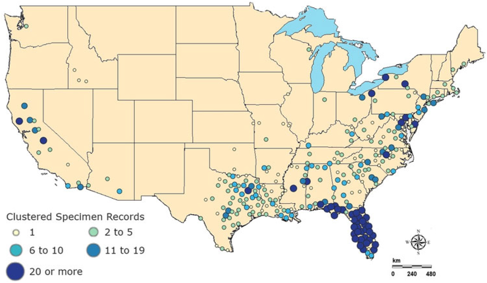
Figure 1. Specimen observation data for 2018 for Hydrilla verticillata (L. f.) Royle from US Geological Survey nonindigenous aquatic species database (US Geological Survey 2018a).
Addressing and understanding the magnitude of the spread of hydrilla is currently a major challenge. To efficiently assess the effects of hydrilla on water quality and overall lake function, the spatial and temporal coverage of this invasive species must be determined. Several different methods, including rake sampling, hydroacoustic survey, mathematical models, and remote sensing, have been applied in an attempt to track and monitor this aquatic invasive plant (Madsen and Wersal Reference Madsen and Wersal2017). The traditional rake-sampling method is reasonably accurate in species differentiation, but it is laborious, time consuming, and cannot display the full extent of hydrilla distribution. Hydroacoustic surveys are expensive and cannot be used to differentiate plant species (Madsen and Wersal Reference Madsen and Wersal2017). Mathematical models are useful for predicting and estimating the current and future invasion of emergent and submerged aquatic invasive plants but are limited in the spatial domain. Therefore, to overcome the aforementioned limitations, researchers have used satellite-based remote-sensing data in studies, which enable relatively less expensive, rapid, frequent, and large-scale monitoring of emergent and submerged aquatic vegetation (SAV) (Ackleson and Klemas Reference Ackleson and Klemas1987; Cho et al. Reference Cho, Mishra, Kirui, Wood and Escalante-Ramirez2012; Cho et al. Reference Cho, Ogashawara, Mishra, White, Kamerosky, Morris, Clarke, Simpson and Banisakher2014; Luo et al. Reference Luo, Li, Ma, Li, Duan, Hu, Qin and Huang2016; Malthus Reference Malthus, Mishra, Ogashawara and Gitelson2017; Rotta et al. Reference Rotta, Mishra, Alcântara and Imai2016; Rotta et al. Reference Rotta, Mishra, Watanabe, Rodrigues, Alcântara and Imai2018). In addition, airborne images were also used for mapping SAV in waterbodies (Hamabata and Kobayashi Reference Hamabata and Kobayashi2002; Hestir et al. Reference Hestir, Khanna, Andrew, Santos, Viers, Greenberg, Rajapakse and Ustin2008). However, compared with data from airborne images, satellite data are widely used for mapping SAV, owing to a relatively large swath that can be imaged, cost-effectiveness, and ease of data acquisition and processing (Yadav et al. Reference Yadav, Yoneda, Susaki, Tamura, Ishikawa and Yamashiki2017).
The earlier application of satellite remote sensing for SAV mapping used commercial satellite products such as images from IKONOS and Quickbird (Jakubauskas et al. Reference Jakubauskas, Peterson, Campbell, Noyelles, Campbell, Penny, Morain and Budge2002; Sawaya et al. Reference Sawaya, Olmanson, Heinert, Brezonik and Bauer2003; Wolter et al. Reference Wolter, Johnston and Niemi2007). For example, Sawya et al. (Reference Sawaya, Olmanson, Heinert, Brezonik and Bauer2003) used IKONOS and QuickBird data to map SAV in lakes of Minnesota. In another study, Wolter et al. (Reference Wolter, Johnston and Niemi2007) used QuickBird data for SAV mapping in the Great Lakes. Though these commercial satellites had higher spatial resolution, such as the 3.2-m multispectral resolution of IKONOS and the 2.4-m multispectral resolution of QuickBird, the data obtained from such satellites may be impractical for frequent monitoring purposes, because of the high cost associated with their small swath coverage. The trend started shifting from commercial satellites to open-source satellite products, especially because Landsat products became freely available in 2008. Since then, several studies used Landsat series sensors, including Thematic Mapper, Enhanced Thematic Mapper, and Operational Land Imager (OLI) for SAV assessment (Brooks et al. Reference Brooks, Grimm, Shuchman, Sayers and Jessee2015; Shuchman et al. Reference Shuchman, Sayers and Brooks2013; Yadav et al. Reference Yadav, Yoneda, Susaki, Tamura, Ishikawa and Yamashiki2017). Not only the cost but the large swath, improved calibration, and higher signal-to-noise ratio of Landsat 8 OLI sensor make it suitable for SAV assessment. There are also some limitations associated with OLI, such as a longer revisit period (16 d) and availability of only few spectral bands, which limits its application in differentiating SAV species. However, there is always a trade-off when selecting a sensor for remote sensing study and, because the scope of this research was limited (e.g., limited funding, lack of Sentinel-2 satellite scene availability corresponding to field sampling period), contemporary images from OLI sensor were the best available option.
Previous satellite-based studies used vegetation indices such as the Normalized Difference Vegetation Index and Floating Algal Index for emergent vegetation mapping (Hu Reference Hu2009; Sawaya et al. Reference Sawaya, Olmanson, Heinert, Brezonik and Bauer2003).These indices are suitable for terrestrial, emergent, and floating vegetation; however, SAV are difficult to detect, because of the optical complexity of the water column (Silva et al. Reference Silva, Costa, Melack and Novo2008), especially in case of hydrilla, which can survive in the water column up to 10 m deep (Dennison et al. Reference Dennison, Orth, Moore, Stevenson, Carter, Kollar, Bergstrom and Batiuk1993; Rotta et al. Reference Rotta, Mishra, Alcântara and Imai2016). One of the major factors that affects detection of SAV when using remote sensing is water clarity (Nelson et al. Reference Nelson, Cheruvelil and Soranno2006). Therefore, past studies used satellite data to estimate water transparency before SAV mapping (Ma et al. Reference Ma, Duan, Gu and Zhang2008; Shuchman et al. Reference Shuchman, Sayers and Brooks2013). However, hydrilla can survive in low-light condition (Bowes et al. Reference Bowes, Van, Garrard and Haller1977; Langeland Reference Langeland1996), and thus requires additional parameters for its accurate detection. Therefore, in addition to water clarity, several studies included depth of SAV colonization and percentage of light at maximum depth of colonization for accurate assessment of SAV species (Canfield et al. Reference Canfield, Langeland, Linda and Haller1985; Chambers and Kalff Reference Chambers and Kalff1985; Dennison Reference Dennison1987; Duarte Reference Duarte1991; Duarte and Kalff Reference Duarte and Kalff1987; Middleboe and Markager Reference Middleboe and Markager1997; Vant et al. Reference Vant, Davies-Colley, Clayton and Coffey1986). However, these studies were based on in situ data only, were limited in time and spatial domain, and were not primarily focused on hydrilla. In the current study, we aimed to integrate in situ and freely available satellite data to develop a model that can aid frequent, rapid, accurate, and synoptic monitoring of hydrilla.
Our overall objective for this study was to develop a model to map the current extent of hydrilla and identify potential areas of growth, using Landsat 8 OLI data and in situ data. A sequential model incorporating in situ water transparency, depth, and light available through the water column was integrated with satellite data to determine the potential locations for submerged hydrilla, following a previous in situ–based study by Kemp et al. (Reference Kemp, Batleson, Bergstrom, Carter, Gallegos and Hunley2004). In the current study, we hypothesized that potential hydrilla location would be low in turbidity and hence, possess sufficient light through water column. We also present seasonal trends in hydrilla extent, using OLI time-series spatial maps. The variability in hydrilla distribution was further analyzed by incorporating physical and meteorological data sets, including water temperature (WT), precipitation, surface runoff, and net inflow data.
The products from this study can be used to assess current hydrilla invasion and facilitate adaptive management by measuring the efficacy of control efforts. To our knowledge, this study is the first to use a comprehensive modeling approach by combining in situ, physical, meteorological, and satellite data to map the extent of submerged hydrilla in the southeastern United States.
Materials and Methods
Study site
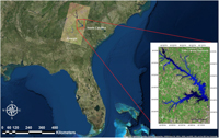
Lake J. Strom Thurmond (hereafter, Lake Thurmond) is a large reservoir (288 km2) that was created by the US Army Corps of Engineers (USACE) in 1951 on the border of Georgia and South Carolina (82°10’ W to 82°39’ W; 33°34’ N to 34°01’ N; Figure 2). The lake is monomictic and has a mean depth of 11 m and a hydraulic retention time of approximately 144 d (USACE 1990). The surface WT ranges from 8 to 30 °C, and thermal and chemical stratification generally occurs in this lake from April to September (Betsill and Van den Avyle Reference Betsill and Van Den Avyle1994). The environmental conditions of this lake (e.g., temperate climate; long, hot summer; substrate type) make it susceptible to proliferation of hydrilla. In 2013, natural resources managers with the USACE and the Georgia and South Carolina Departments of Natural Resources (DNRs) estimated hydrilla distribution spans approximately 11,000 acres of Lake Thurmond, which is about 15% of Lake Thurmond’s total 71,000 acres of water (USACE 2014). Most importantly, a disease called avian vacuolar myelinopathy, which kills local bird species, has been positively identified in hydrilla of Lake Thurmond, making it a high priority in terms of management (Wilde et al. Reference Wilde, Johansen, Wilde, Jiang, Bartelme and Haynie2014). The USACE struggles to produce rapid and accurate estimates of hydrilla density and coverage in Lake Thurmond. Therefore, this study was designed to develop accurate estimations that will allow the USACE to cut costs associated with time-intensive manual surveying. Results of this work will also aid assessing the effectiveness of management and control efforts at Lake Thurmond and other inland water bodies.

Figure 2. Study area map showing satellite imagery of Lake Thurmond derived from Landsat 8 Operational Land Imager (OLI) (band 6: SWIR 1; band 5: NIR; band 4: Red).
The overall process and data involved in different stages of this study are shown in Figure 3. The major components in the process included collecting in situ data, downloading satellite data, preprocessing for data extraction, model calibration and validation, and implementing the model to predict hydrilla extent and the seasonal variability through a time-series analysis. Each component is described concisely in the following sections.
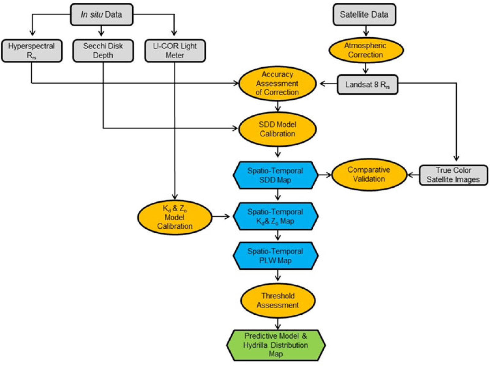
Figure 3. Overall methodology showing various processes involved in integrating in situ and satellite data to develop the hydrilla distribution predictive model. Kd, light-attenuation coefficient; PLW, percentage of light available through the water column; Rrs, remote sensing reflectance; SDD, Secchi disk depth; Zc, maximum depth of hydrilla colonization.
Data acquisition
The following in situ data were collected from Lake Thurmond on June 21, 2016: remote sensing reflectance (Rrs) was measured with an HR-1024i spectroradiometer (wavelength range: 340 to 2500 nm with 1.5-nm spectral resolution; Spectra Vista Corp., Poughkeepsie, NY, USA), light transparency was measured in meters as Secchi disk depth (SDD), and light available was measured through the water column (µmol s−1 m−2) with an underwater quantum sensor LI-192 (LI-COR Inc., Lincoln, NE, USA). The maximum depth of colonization (Zc) of submerged hydrilla was measured using the frame on which the underwater quantum sensor was mounted. Data from 15 different sampling locations were included in the in situ data set, and coordinates were acquired for each location using a Garmin eTrex® ×20 handheld global positioning system. The spectroradiometer collected radiance measurements for wavelengths between 350 and 2,500 nm. The standard procedure was followed to collect SDD (Green et al. Reference Green, Herron and Gold2010). The underwater quantum sensor was used to measure downwelling, photosynthetically active radiation (PAR) (µmol s−1 m−2) at depth intervals of 0.5 m. Parallel to in situ data, satellite data from the Landsat 8 OLI were acquired from the USGS Earth Explorer website on the same date corresponding to the study area and in situ data measurements. Atmospheric and lake conditions were assumed to be the same for in situ and satellite remote-sensing data because the two data sets were collected within 4 h and the atmospheric condition was stable throughout the day (i.e., there were no thunderstorms or scattered clouds). Table 1 includes the description of the satellite and meteorological data used in this study. Landsat 8 OLI scenes from October 2015 to June 2016 were downloaded to examine the seasonal variability and hydrilla extent. The seasonal variability in hydrilla extent was further analyzed by incorporating physical and meteorological data from the North American Land Data Assimilation System (NLDAS), including monthly surface runoff (NLDAS_NOAH0125_M v002) (kg m−2) and precipitation (NLDAS_FORA0125_M v002) (kg m−2) between June 2015 and July 2016, acquired from NASA’s Giovanni website (NASA Giovanni 2017). The spatial resolution of both products is 0.125 ×0.125°. Monthly mean WT data were collected near Plum Branch in Lake Thurmond for 2011 to 2017 from the USGS website (US Geological Survey 2018b). In addition, 16 years of net inflow data for Lake Thurmond were downloaded from the USACE Savannah Water District Management website for assessing the impact of net inflow on seasonal variability of hydrilla extent (USACE 2018).
Table 1. Summary of the satellite, physical, and meteorological data used in this study.
a Abbreviations: –, no data; NLDAS, North American Land Data Assimilation System; OLI, Operational Land Imager.
Model calibration
Atmospheric Correction of Landsat 8 OLI Imagery. Preprocessing of satellite data was required before comparing them with in situ data to correct for any atmospheric interference caused in the signal received by the sensor. Therefore, Landsat 8 OLI imagery was corrected for Rayleigh, Fresnel, and aerosol noise contributions following the logic outlined by Mishra et al. (Reference Mishra, Narumalani, Rundquist and Lawson2005) and Dash et al. (Reference Dash, Walker, Mishra, D’Sa and Ladner2012), modified for the OLI sensor. This algorithm systematically converts the 16-bit top-of-atmosphere brightness values into Rrs and outputs atmospherically corrected data of water pixels.
Data Extraction and Correlation Analysis. The atmospherically corrected image was imported to NASA’s SeaDAS software (https://seadas.gsfc.nasa.gov/), which extracted Rrs values from pixels containing the 15 in situ data locations. To validate the accuracy of atmospheric correction, Landsat 8 OLI Rrs values from band 1 (440 nm) through band 5 (865 nm) were compared with in situ Rrs values at equal wavelengths. After accuracy assessment, Rrs data from OLI were correlated with in situ SDD measurements corresponding to all 15 sampling locations to reparameterize an SDD model by Fuller et al. (Reference Fuller, Aichele and Minnerick2004). Fuller et al. (Reference Fuller, Aichele and Minnerick2004) tested various band combinations of Landsat 5 Thematic Mapper and Landsat 7 Enhanced Thematic Mapper+ data to develop the SDD model. Therefore, similar spectral bands from the OLI sensor (bands 2, 3, and 4) were used in this study to reparameterize the SDD model.
The SDD model was also useful to determine the other two parameters, Kd and Zc, of submerged vegetation in several previous studies (Chambers and Kalff Reference Chambers and Kalff1985; Dennison Reference Dennison1987; Duarte Reference Duarte1991; Duarte and Kalff Reference Duarte and Kalff1987; Middleboe and Markager Reference Middleboe and Markager1997; Rotta et al. Reference Rotta, Mishra, Alcântara and Imai2016; Vant et al. Reference Vant, Davies-Colley, Clayton and Coffey1986). These two parameters (Kd and Zc) were necessary for developing the hydrilla distribution model. Therefore, we examined the relationship between SDD and these two parameters.
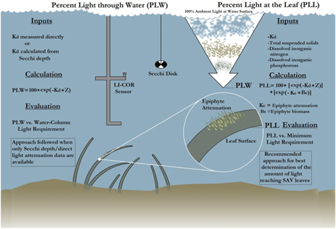
First, the Kd derived from PAR measurements [Kd (PAR)], derived from the LI-COR sensor, was correlated with SDD. Similarly, the Zc of hydrilla was correlated with SDD at 15 sampling sites. The goal for establishing a relationship among these three parameters was to determine the PLW following the methodology described by Kemp et al. (Reference Kemp, Batleson, Bergstrom, Carter, Gallegos and Hunley2004) (Figure 4). Kemp et al. (Reference Kemp, Batleson, Bergstrom, Carter, Gallegos and Hunley2004) presented two approaches for calculating the PLW and percentage of light at leaf level (PLL) (Figure 4; Equations 1 and 2). However, epiphyte data were not available for this study; therefore, only the PLW approach was used for creating the hydrilla distribution model, as follows:
 $${\rm{PLW }} = {\rm{ 1}}00{\rm{ }} \times {\rm{ exp }}\left[ {\left( { - {{\rm{K}}_{\rm{d}}} \times {\rm{ Z}}} \right)} \right]$$
([1])
$${\rm{PLW }} = {\rm{ 1}}00{\rm{ }} \times {\rm{ exp }}\left[ {\left( { - {{\rm{K}}_{\rm{d}}} \times {\rm{ Z}}} \right)} \right]$$
([1])
 $${\rm{PLL }} = {\rm{ 1}}00 \times {\rm{ exp}}\left[ {\left( { - {{\rm{K}}_{\rm{d}}} \times {\rm{ Z}}} \right)} \right]{\rm{ }} \times {\rm{ exp }}\left[ {\left( { - {{\rm{K}}_{\rm{e}}} \times {\rm{ }}{{\rm{B}}_{\rm{e}}}} \right)} \right]$$
([2])
$${\rm{PLL }} = {\rm{ 1}}00 \times {\rm{ exp}}\left[ {\left( { - {{\rm{K}}_{\rm{d}}} \times {\rm{ Z}}} \right)} \right]{\rm{ }} \times {\rm{ exp }}\left[ {\left( { - {{\rm{K}}_{\rm{e}}} \times {\rm{ }}{{\rm{B}}_{\rm{e}}}} \right)} \right]$$
([2])
where Ke is epiphyte attenuation, Be is epiphyte biomass, and Z is depth. Equations 1 and 2 were developed on the basis of SAV species other than hydrilla. But because hydrilla can grow longer in lower-light environments, several threshold values were experimented for PLW during the model development to capture the full extent of submerged hydrilla in Lake Thurmond.
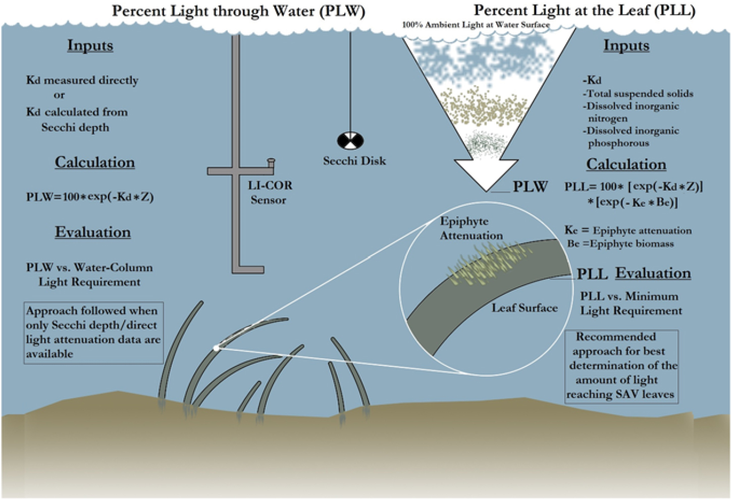
Figure 4. The process involved in calculating percentage of light through water (PLW) and percentage of light at leaf (PLL) [re-created from the study by Kemp et al. (Reference Kemp, Batleson, Bergstrom, Carter, Gallegos and Hunley2004)]. Kd, light-attenuation coefficient; SAV, submerged aquatic vegetation; Z, depth.
Qualitative validation and seasonal variability in hydrilla extent
The USACE carried out time and labor-intensive field surveys over multiple days during September and October 2015 to create a map showing known locations of hydrilla distribution in Lake Thurmond. This field survey was accomplished with the help of two environmental agencies (i.e., Georgia Department of Natural Resources and South Carolina Department of Natural Resources) and University of Georgia’s Warnell School of Forestry and Natural Resources (USACE 2016). During this survey, the entire lake was divided into nine separate survey routes and sample points were established along the lake’s shoreline. These sampling points were surveyed for the presence or absence of hydrilla, using a two-sided metal garden rake with a rope.
After the field survey, the hydrilla locations were mapped in ArcView software (Esri, Redlands, CA). This map produced by the USACE was used as a reference to qualitatively validate the satellite-based hydrilla distribution map produced using the predictive model that used same-month Landsat 8 OLI data from 2015. After the qualitative validation was completed, additional Landsat imagery from different months was used to observe spatiotemporal distribution of hydrilla and its seasonal trend. In addition, spatial maps with four input parameters (i.e., SDD, Kd, Zc, and PLW) were analyzed in parallel and used to create final hydrilla presence and absence maps. Furthermore, data on seasonal variability in meteorological and physical factors corresponding to Lake Thurmond were analyzed to determine the factors’ possible impact on hydrilla distribution.
Results and Discussion
Model calibration
Landsat 8 OLI–derived Rrs spectra corresponding to 15 sampling locations are shown in Figure 5a. Variability in Rrs spectra was attributed to differences in water transparency level at different sampling locations and was used in reparameterizing the SDD model developed by Fuller et al. (Reference Fuller, Aichele and Minnerick2004). The reparameterized SDD model (Equation 3) showed significant correlation (r = 0.78; P < 0.01) between OLI visible bands (i.e., bands 2, 3, and 4) and in situ SDD measurements:
 $${\rm{ln}}\left( {{\rm{SDD}}} \right){\rm{ }} = {\rm{ }}\left( { - {\rm{95}}.{\rm{534 }} \times {\rm{ band 2}}} \right){\rm{ }} + {\rm{ }}\left( {{\rm{171}}.{\rm{4}}0{\rm{69 }} \times {\rm{ band 3}}} \right){\rm{ }} - {\rm{ }}\left( {{\rm{212}}.{\rm{118 }} \times {\rm{ band 4}}} \right){\rm{ }} + {\rm{ }}0.{\rm{841359}}$$
([3])
$${\rm{ln}}\left( {{\rm{SDD}}} \right){\rm{ }} = {\rm{ }}\left( { - {\rm{95}}.{\rm{534 }} \times {\rm{ band 2}}} \right){\rm{ }} + {\rm{ }}\left( {{\rm{171}}.{\rm{4}}0{\rm{69 }} \times {\rm{ band 3}}} \right){\rm{ }} - {\rm{ }}\left( {{\rm{212}}.{\rm{118 }} \times {\rm{ band 4}}} \right){\rm{ }} + {\rm{ }}0.{\rm{841359}}$$
([3])
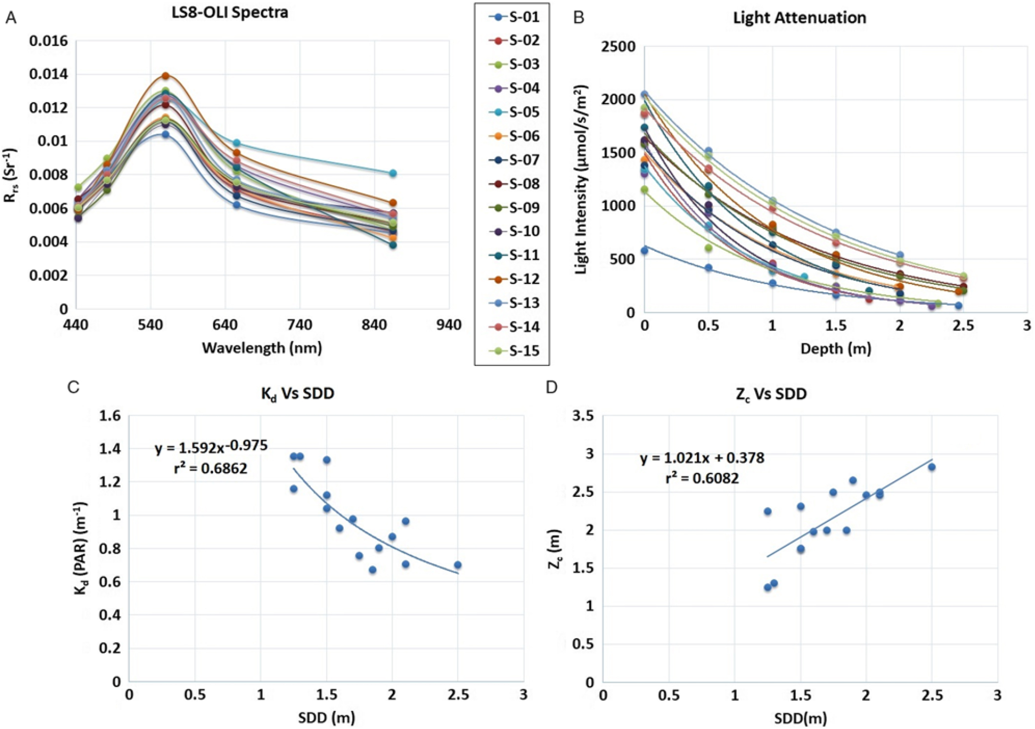
Figure 5. (a) Landsat 8 (LS8) Operational Land Imager (OLI) derived remote sensing reflectance (Rrs) spectra corresponding to various sampling locations. (b) LI-COR meter–derived light attenuation with respect to water column depth. (c) Correlation between light-attenuation coefficient (Kd) derived from photosynthetically active radiation (PAR) measurements [Kd (PAR)] derived from LI-COR data and in situ Secchi disk depth (SDD). (d) Correlation between maximum depth of hydrilla colonization (Zc) and SDD.
LI-COR–derived light attenuation in water column is shown in Figure 5b. The light-attenuation equations for each sampling location (S-01 to S-15) are presented in Table 2 and were used for deriving Kd (PAR) for each location. A significant difference in light level at the surface for sampling location S-01 was observed as a result of cloud cover during measurement (Figure 5b; Table 2). A significant inverse correlation (r = 0.82; P < 0.001) was observed between Kd (PAR) derived from LI-COR measurements and in situ SDD (Figure 5c; Equation 4):
 $${{\rm{K}}_{\rm{d}}}\left( {{\rm{PAR}}} \right){\rm{ }} = {\rm{ 1}}.{\rm{592 }} \times {\rm{ }}{\left( {{\rm{SDD}}} \right)^{ - 0.{\rm{975}}}}$$
([4])
$${{\rm{K}}_{\rm{d}}}\left( {{\rm{PAR}}} \right){\rm{ }} = {\rm{ 1}}.{\rm{592 }} \times {\rm{ }}{\left( {{\rm{SDD}}} \right)^{ - 0.{\rm{975}}}}$$
([4])
Table 2. Summary of LI-COR meter reading, Kd (PAR), derived from the light-attenuation equation, Zc, and SDD measurement recorded at each sampling location.
a Abbreviations: Kd (PAR), light-attenuation coefficient derived from photosynthetically active radiation measurements; I0, light measured at water surface; PAR, photosynthetically active radiation; SDD, Secchi disk depth; Zc, maximum depth of hydrilla colonization.
The inverse correlation between Kd and SDD confirmed that light attenuation was higher for the sampling locations with lower water transparency. Previous studies also showed an inverse relationship between Kd and SDD (Table 3).
Table 3. Previous studies that found a relationship among Kd, SDD, and Zc, using in situ data.
a Abbreviation: Kd, light-attenuation coefficient; SDD, Secchi disk depth; Zc, maximum depth of hydrilla colonization.
The next stage in the hydrilla predictive model was to establish a relationship between SDD and Zc. A significant positive correlation (r = 0.78; P < 0.001) was observed between SDD and Zc (Figure 5d; Equation 5), which suggested that hydrilla can colonize deeper if the transparency level in water column remains high.
 $${{\rm{Z}}_{\rm{c}}} = {\rm{ 1}}.0{\rm{21 }} \times {\rm{ }}\left( {{\rm{SDD}}} \right){\rm{ }} + {\rm{ }}0.{\rm{378}}$$
([5])
$${{\rm{Z}}_{\rm{c}}} = {\rm{ 1}}.0{\rm{21 }} \times {\rm{ }}\left( {{\rm{SDD}}} \right){\rm{ }} + {\rm{ }}0.{\rm{378}}$$
([5])
Similar positive correlations between SDD and Zc were reported in previous studies (Table 3).
With Kd (PAR) and Zc values available, the next step was to estimate PLW following the logic of Kemp et al. (Reference Kemp, Batleson, Bergstrom, Carter, Gallegos and Hunley2004) (Equation 1). However, PLW estimates alone were not enough to capture the full extent of submerged hydrilla accurately. Therefore, a minimum threshold limit of 10 m for both PLW and depth was implemented to mask out the hydrilla location. A 10-m threshold was chosen because hydrilla typically is not found beyond that depth in Lake Thurmond, according to the USACE. Past studies reported different threshold values of minimum light requirement for SAV species, depending on the types of body of water, such as tidal fresh, oligohaline, mesohaline, and polyhaline (Batiuk et al. Reference Batiuk, Orth, Moore, Stevenson, Dennison, Staver, Carter, Rybicki, Hickman, Kollar and Bieber1992; Dennison et al. Reference Dennison, Orth, Moore, Stevenson, Carter, Kollar, Bergstrom and Batiuk1993; Kemp et al. Reference Kemp, Batleson, Bergstrom, Carter, Gallegos and Hunley2004) (Table 4). In this study, after experimenting with various threshold values, 13% PLW was used as the minimum light-requirement threshold to predict hydrilla location. The 13% PLW threshold was also found suitable in another study for SAV species in tidal freshwater with a growing season phenology from April to October (Kemp et al. Reference Kemp, Batleson, Bergstrom, Carter, Gallegos and Hunley2004) (Table 4). Lake Thurmond also falls under the freshwater category and has a similar growing season for hydrilla; hence, the predictive model using a similar threshold developed in this study captured the full extent of hydrilla distribution and its seasonal variability.
Table 4. The growing season of SAV and recommended water-column light requirements for different types of water.a
b Abbreviation: SAV, submerged aquatic vegetation.
Qualitative validation and seasonal variability in hydrilla extent
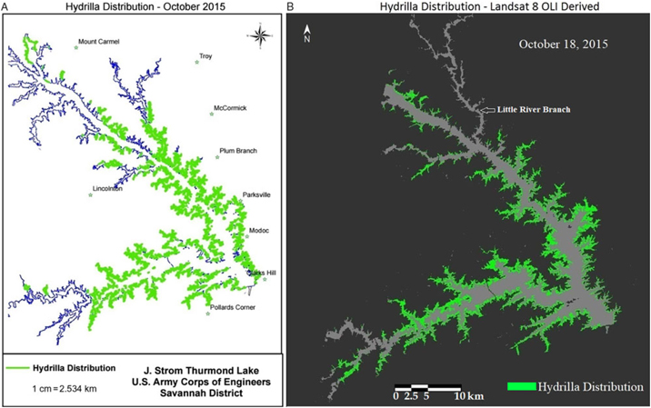
Qualitative comparison between the hydrilla distribution map created by the USACE and the Landsat 8–derived predictive map revealed a similar distribution extent for October 2015, which is the peak growing season for hydrilla in Lake Thurmond (Figure 6). One exception was the highly turbid region of the Little River branch, highlighted in Figure 6b, where the PLW model showed minimum hydrilla presence. This could be because the model result was derived from one particular date (i.e., October 18, 2015, whereas the USACE hydrilla distribution map corresponds to the extensive field survey conducted in September and October 2015. The one-time hydrilla map produced by the USACE involved significant manpower [people from three agencies were involved in the field survey (USACE 2016)], time, and money. In contrast, the model developed in this study is a one-time investment (the entire project cost was approximately $10,000) that can produce hydrilla distribution maps frequently and within hours once the satellite data become available—without any additional cost.
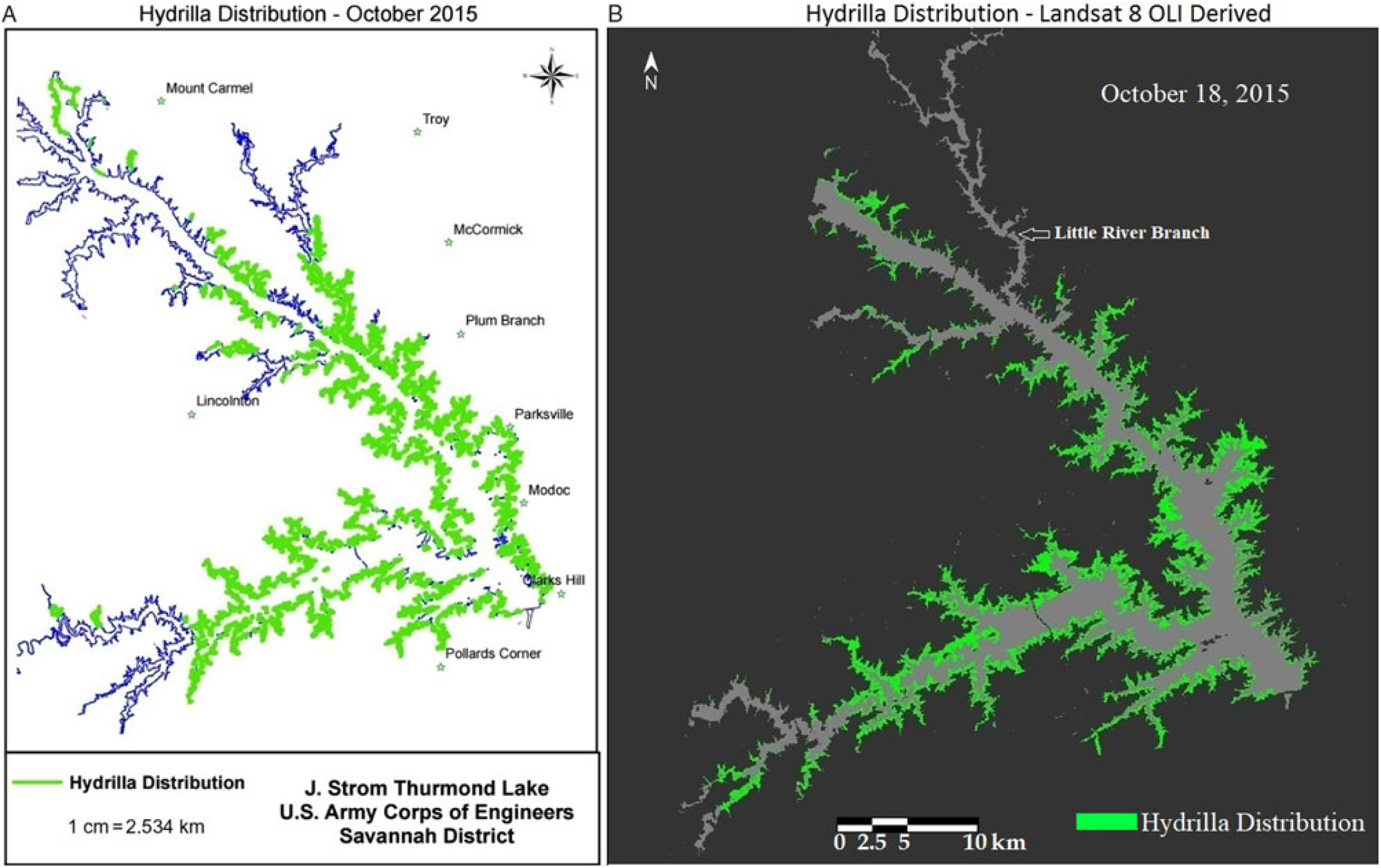
Figure 6. (a) Map of Lake Thurmond created by the US Army Corps of Engineers showing known locations of hydrilla along the shoreline. (b) Landsat 8 Operational Land Imager (OLI)-derived map showing predicted hydrilla locations.
After qualitative validation for the month of October, Landsat 8 OLI data from subsequent months were analyzed to determine hydrilla extent. The qualitative analysis of results corresponding to SDD and respective true-color Landsat images suggested that areas with high turbidity (indicated by a brownish color in true-color images) have low SDD and areas with clear water (dark blue in true-color images) have high SDD values (Figure 7). These results validated the SDD model.
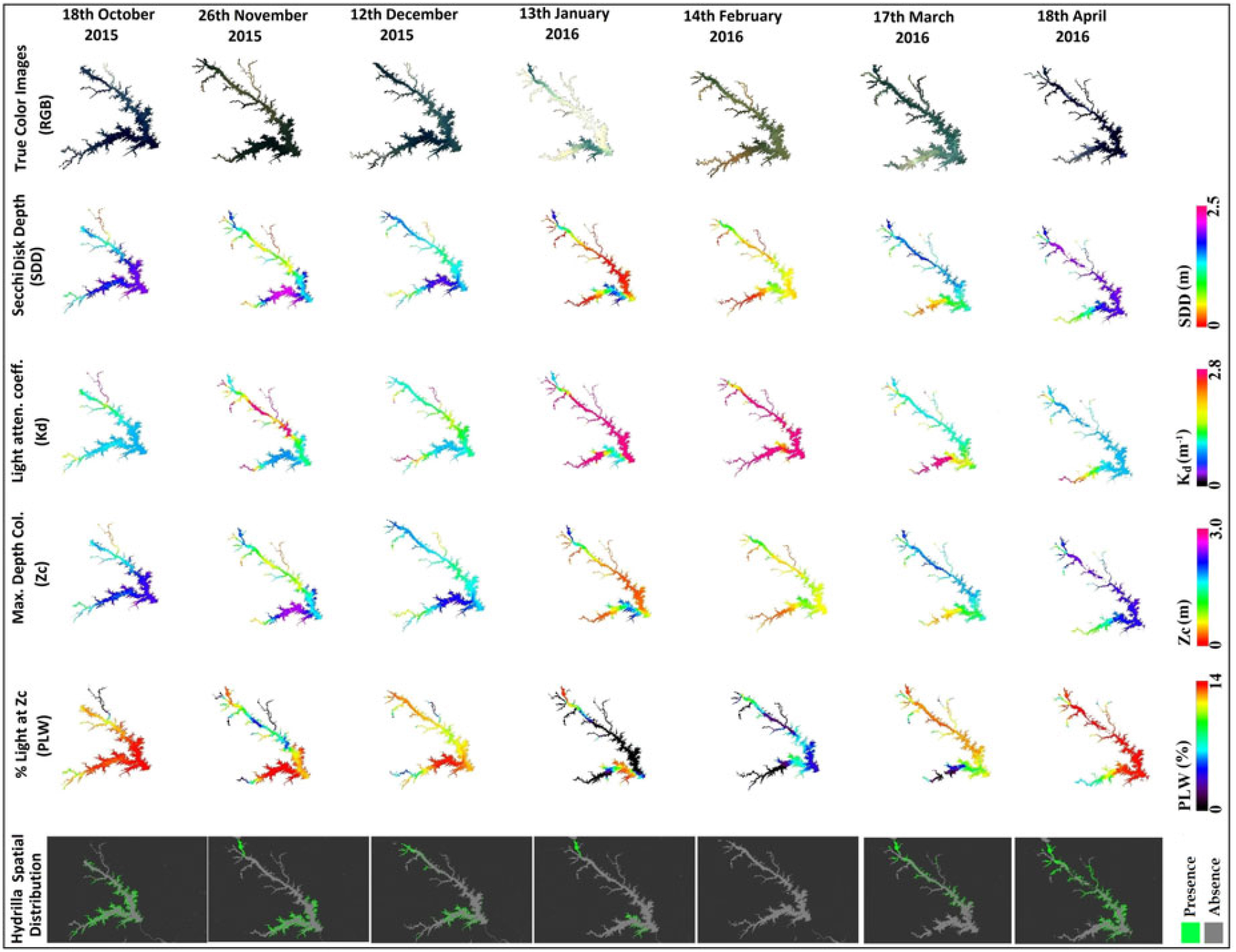
Figure 7. Spatiotemporal variability in Landsat 8 Operational Land Imager–derived true-color images, Secchi disk depth (SDD), light-attenuation coefficient (Kd) derived from photosynthetically active radiation, maximum depth of hydrilla colonization (Zc), percentage of light through water (PLW) at Zc, and hydrilla distribution (presence/absence) maps. RGB, red, green, blue.
The second parameter in the hydrilla predictive model, Kd (PAR), had an inverse relationship with SDD; hence, the turbid areas had higher Kd (PAR) values compared with clear water, for which Kd (PAR) values were lower. Spatiotemporal Zc maps showed a similar pattern to SDD, validating the linear calibration result found between SDD and Zc (Figures 5d and 7).
The SDD and Zc spatiotemporal maps captured the dominant locations of hydrilla (Figure 7, pink represents water with high SDD and Zc values) but not the full extent of hydrilla distribution. However, the PLW spatiotemporal maps [which take into account Kd (PAR) and Zc, derived from SDD values] were more suitable to show the full extent of hydrilla distribution. The spatiotemporal PLW maps at Zc showed higher values for transparent regions and lower values for turbid parts of the lake. In this process, deeper parts of the lake also had high PLW values because of high transparency. This caused the model to predict hydrilla in deeper waters than it can inhabit. Therefore, a 10-m depth mask was applied after the 13% threshold value of PLW at Zc to produce final hydrilla distribution maps. The final maps displayed the spatiotemporal distribution of hydrilla at full extent (Figure 7).
From analysis of the final hydrilla distribution maps, it was observed that hydrilla typically starts growing during April in the northernmost waters of the lake, then spreads southward in May and June. Hydrilla reached peak distribution during October, began retreating in the following months, and disappeared completely in February. These results suggested that turbidity could be a limiting factor for hydrilla survival, because the lowest light levels were observed during February, due to high turbidity. Therefore, physical and meteorological factors, including surface runoff, precipitation, and net water-inflow data were included in additional analysis; these factors are known to affect turbidity level of the lake and subsequently light availability in the water column. WT data were also included in additional analysis because it could be another major factor controlling the seasonality of hydrilla.
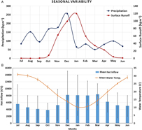
Seasonal analysis of precipitation and surface runoff for Lake Thurmond between July 2015 and June 2016 revealed that December 2015 was associated with the highest level of precipitation (257.51 kg m−2), which brought heavy surface runoff during this month (99.46 kg m−2) and January (surface runoff, 120.01 kg m−2) (Figure 8a). The surface runoff was negligible during summer months (June to September), because of the dry surface coupled with low precipitation; hence, the turbidity level in Lake Thurmond was observed to be lowest in the following month, October 2015 (Figure 7), allowing sufficient light to be available in the water column for proliferation of hydrilla. However, surface runoff started increasing in November 2015, after the precipitation; thus, the turbidity level also started increasing and reached its highest level during January and February 2016. With limited light conditions in the water column for turbid regions of the lake, and the extent of hydrilla began diminishing after October and reached its lowest level in February 2016 (Figure 7).
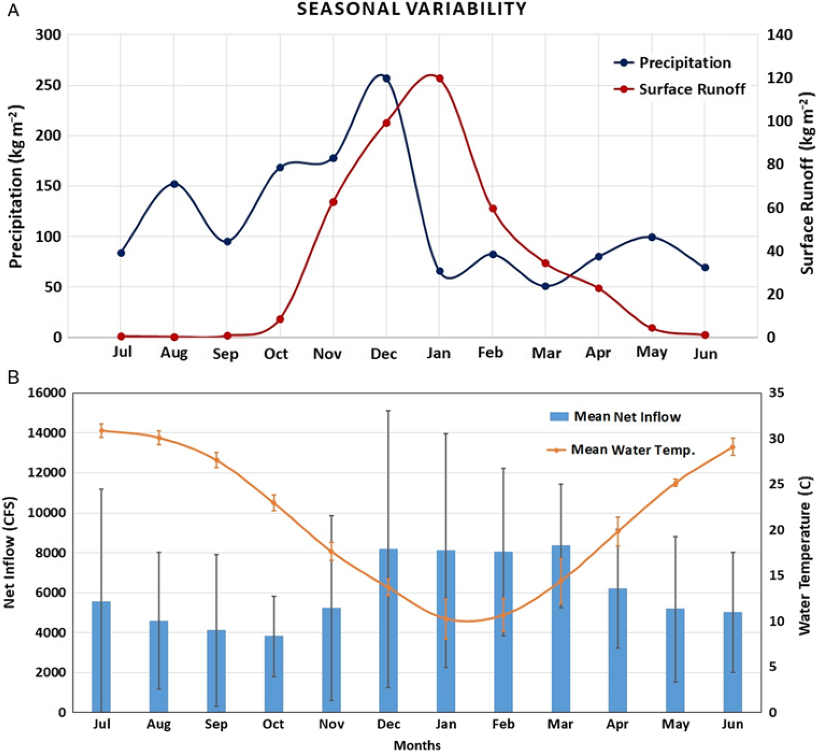
Figure 8. (a). Monthly variability in precipitation and surface runoff between July 2015 and June 2016 for Lake Thurmond. (b) Monthly net inflow data presented for 2001 to 2016. The mean net inflow value for each month was presented with standard deviation as error bars (net inflow data were downloaded from the US Army Corps of Engineers Savannah Water District Management website [USACE 2018]). Monthly mean water temperature data are presented for Lake Thurmond corresponding to a site near Plum Branch, SC, for 2011 to 2017 (US Geological Survey 2018b).
Another parameter corresponding to the Lake Thurmond, monthly net inflow (2001 to 2016), was analyzed (Figure 8). Again, the lowest mean net inflow (3,821.29 CFS) occurred in October, compared to other months (Figure 8b). In addition, a seasonal trend in mean monthly net inflow increased from November through March and then decreased from April to October (Figure 8b). This was in contrast to the seasonal trend found for hydrilla distribution in Lake Thurmond, where hydrilla extent started decreasing from November through March and then started to grow again in April and reached peak level in October. Therefore, apart from light availability in the water column, net inflow can also affect the proliferation of hydrilla in Lake Thurmond. Furthermore, analysis of WT data revealed July as the warmest month (mean WT, 30.91 C) and January as the coldest (mean WT, 10.29 C) (Figure 8b). It has been suggested in previous studies that WT range should be between 20 and 27 C for optimum growth of hydrilla, and the maximum temperature hydrilla can withstand is 30 C (Jain and Kalamdhad Reference Jain and Kalamdhad2018; Steward and Van Reference Steward and Van1987). Optimum growth of hydrilla in Lake Thurmond was observed during October, when temperature range was within the 20–27 C range (mean WT, 22.99 C). The WT dropped sharply after October resulting in significant reduction in hydrilla spatial extent. These results show WT is a major controlling factor associated with seasonality of hydrilla distribution in Lake Thurmond.
Overall, the methodology developed in this study was successful in accurately mapping hydrilla, projecting its seasonal extent, and, therefore, predicting potential areas of growth. The model predicts ideal habitat for hydrilla in waters featuring high SDD, low values of Kd (PAR), and, consequently, both high Zc and PLW. However, due to limited spectral bands, Landsat 8 OLI is unable to isolate hydrilla from other species of aquatic vegetation. Therefore, the models developed in this study will be most useful in bodies of water where hydrilla is known to be the most prevalent species of aquatic vegetation. Future work could use hyperspectral satellites to measure hydrilla at the wavelengths where it is most easily identified: 725 and 818 nm (Blanco et al. Reference Blanco, Qu and Roper2012). The use of a hyperspectral sensor could potentially differentiate hydrilla from other submerged vegetation, which would be useful in lakes where hydrilla is not the dominant aquatic vegetation species. Another limitation with Landsat 8 OLI data is the satellite’s poor revisit time of 16 days. The European Space Agency’s Sentinel 2-MSI satellite sensor has similar band characteristics as Landsat 8 OLI but with higher temporal (5-day revisit period) and spatial (up to 10 m) resolution (Page et al. Reference Page, Kumar and Mishra2018). In future studies, Sentinel-2 data could be used to further validate the results observed in this research until space-borne hyperspectral data become available. Although the predictive model developed in this study can be used to accurately map and predict hydrilla distribution, it could be refined further by incorporating more data. For example, nutrient and epiphyte biomass data for the study area could be used to derive PLL, which would provide a more accurate estimation of hydrilla distribution, because this species can grow in low-light conditions (Kemp et al. Reference Kemp, Batleson, Bergstrom, Carter, Gallegos and Hunley2004). Additional improvements could be made by incorporating benthic substrate and soil-type data.
Mapping of hydrilla spatial extent at regular intervals could be highly useful for lake management. The annual maintenance cost for invasive aquatic weeds within the United States has been estimated to be approximately $110 million (Pimentel et al. Reference Pimentel, Zuniga and Morrison2005). For hydrilla management alone, Florida state agencies have spent approximately $250 million over the past 30 years in Florida waters (Madsen and Wersal Reference Madsen and Wersal2017). A significant proportion of the money can be saved by implementing effective monitoring techniques such as the one developed in this study, which can help identify the potential locations of hydrilla as early as possible and be used to evaluate the success or failure of past biological control projects. The model developed in this study was a one-time investment of approximately $10,000 that can save time and money in routine monitoring of hydrilla as soon as satellite imagery becomes available. In the past, it took more than a month to produce a one-time hydrilla distribution map for Lake Thurmond with the help of multiple environmental agencies performing labor intensive and expensive field work. Freely available satellite data now can be processed in hours with open-access image-processing tools to prepare such maps. Currently, the USACE has the geographic information system expertise to run the hydrilla model developed in this study with simple instruction, and this has already been communicated personally with the USACE at the Lake Thurmond office. The model can be integrated into an open-access, cloud-based interface (i.e., Google Earth Engine tool) so anyone can use and share it with others. Although the results presented in this study were specific to Lake Thurmond, the methodology can be replicated to other inland water bodies. For smaller waterbodies, Sentinel 2-MSI (10 m), RapidEye (5 m), PlanetScope (3 m), or WorldView-3 (1.24 m) data can also be used. Management agencies can use the satellite-derived products not only to plan future removal efforts of hydrilla but also to evaluate and adaptively change their current mitigation efforts.
Author ORCIDs
Abhishek Kumar 0000-0002-0956-1766
Acknowledgements
The authors would like to thank the NASA DEVELOP National Program and the Geography Department at the University of Georgia for funding and supporting this project. No conflicts of interest have been declared. The authors are very thankful to the US Army Corps of Engineers for their tremendous help during field work. We thank NASA DEVELOP team members at the University of Georgia, including Pradeep Kumar Ragu Chanthar, Brandon Hays, Linli Zhu, Wuyang Cai, Elizabeth Dyer, and Peter Hawman, for their contribution. The authors also acknowledge Dr. Kenton Ross and Amanda Clayton from the NASA DEVELOP National Program Office for their help editing this manuscript. Special thanks to Roger Bledsoe for his help in re-creating the Kemp et al. (Reference Kemp, Batleson, Bergstrom, Carter, Gallegos and Hunley2004) figure included in this study. This material is based on work supported by NASA through contract NNL11AA00B and cooperative agreement NNX14AB60A.