


1 Introduction
1.1 Internal flows in soft-walled channels/tubes
The effect of soft walls on the transition to turbulence in an internal flow at small dimensions and Reynolds numbers was first studied by Lahav, Eliezer & Silberberg (Reference Lahav, Eliezer and Silberberg1973) and Krindel & Silberberg (Reference Krindel and Silberberg1979). They found that the transition Reynolds number for the laminar–turbulent transition is lower than the value of 2100 for the rigid tube and that the transition Reynolds number decreases as the elasticity modulus of the wall of the tube decreases. This motivated a series of theoretical linear stability analyses and experiments on the stability of internal flows in soft tubes and channels, of interest in physiological and microfluidic applications (Kumaran Reference Kumaran2000, Reference Kumaran, Carpenter and Pedley2003, Reference Kumaran2015; Shankar Reference Shankar2015). The transition Reynolds number is a function of the dimensionless parameter
 $\unicode[STIX]{x1D6F4}=(\unicode[STIX]{x1D70C}GR^{2}/\unicode[STIX]{x1D702}^{2})$
, which is the ratio of the elastic stresses in the solid and the viscous stresses in the fluid, and which is independent of the flow velocity. Here,
$\unicode[STIX]{x1D6F4}=(\unicode[STIX]{x1D70C}GR^{2}/\unicode[STIX]{x1D702}^{2})$
, which is the ratio of the elastic stresses in the solid and the viscous stresses in the fluid, and which is independent of the flow velocity. Here,
 $R$
is the characteristic conduit dimension,
$R$
is the characteristic conduit dimension,
 $G$
is the shear modulus of wall material,
$G$
is the shear modulus of wall material,
 $\unicode[STIX]{x1D702}$
and
$\unicode[STIX]{x1D702}$
and
 $\unicode[STIX]{x1D70C}$
are the fluid viscosity and density respectively.
$\unicode[STIX]{x1D70C}$
are the fluid viscosity and density respectively.
1.1.1 Stability analyses
The flow past a viscoelastic surface could become unstable even in the limit of zero Reynolds number if the elasticity of the walls was made sufficiently small (Kumaran, Fredrickson & Pincus Reference Kumaran, Fredrickson and Pincus1994; Kumaran Reference Kumaran1995; Gkanis & Kumar Reference Gkanis and Kumar2003, Reference Gkanis and Kumar2005; Shankar & Kumar Reference Shankar and Kumar2004; Chokshi & Kumaran Reference Chokshi and Kumaran2008) when the dimensionless velocity
 $(V\unicode[STIX]{x1D702}/GR)$
exceeds a threshold value. Here,
$(V\unicode[STIX]{x1D702}/GR)$
exceeds a threshold value. Here,
 $V$
is the average flow velocity. At high Reynolds number, different types of instability have been predicted. In the high Reynolds number ‘inviscid’ instability (Kumaran Reference Kumaran1996; Shankar & Kumaran Reference Shankar and Kumaran1999, Reference Shankar and Kumaran2000; Gaurav & Shankar Reference Shankar2009, Reference Shankar2010), viscous effects are important in an internal critical layer of thickness
$V$
is the average flow velocity. At high Reynolds number, different types of instability have been predicted. In the high Reynolds number ‘inviscid’ instability (Kumaran Reference Kumaran1996; Shankar & Kumaran Reference Shankar and Kumaran1999, Reference Shankar and Kumaran2000; Gaurav & Shankar Reference Shankar2009, Reference Shankar2010), viscous effects are important in an internal critical layer of thickness
 $Re^{-1/3}$
within the flow, and the transition Reynolds number increases proportional to
$Re^{-1/3}$
within the flow, and the transition Reynolds number increases proportional to
 $\unicode[STIX]{x1D6F4}^{1/2}$
. In the wall mode instability at high Reynolds number, viscous forces are comparable to inertial forces in a layer of thickness
$\unicode[STIX]{x1D6F4}^{1/2}$
. In the wall mode instability at high Reynolds number, viscous forces are comparable to inertial forces in a layer of thickness
 $Re^{-1/3}$
at the wall (Kumaran Reference Kumaran1998; Shankar & Kumaran Reference Shankar and Kumaran2001, Reference Shankar and Kumaran2002; Chokshi & Kumaran Reference Chokshi and Kumaran2009). The transition Reynolds number scales as
$Re^{-1/3}$
at the wall (Kumaran Reference Kumaran1998; Shankar & Kumaran Reference Shankar and Kumaran2001, Reference Shankar and Kumaran2002; Chokshi & Kumaran Reference Chokshi and Kumaran2009). The transition Reynolds number scales as
 $\unicode[STIX]{x1D6F4}^{3/4}$
, and the mechanism of destabilisation is the shear work done at the surface due to the coupling between the mean strain rate and the surface displacement in the tangential velocity boundary condition at the interface.
$\unicode[STIX]{x1D6F4}^{3/4}$
, and the mechanism of destabilisation is the shear work done at the surface due to the coupling between the mean strain rate and the surface displacement in the tangential velocity boundary condition at the interface.
1.1.2 Transition in experiments
This low Reynolds number instability has been observed in experiments (Kumaran & Muralikrishnan Reference Kumaran and Muralikrishnan2000; Muralikrishnan & Kumaran Reference Muralikrishnan and Kumaran2002; Eggert & Kumar Reference Eggert and Kumar2004; Shrivastava, Cussler & Kumar Reference Shrivastava, Cussler and Kumar2008), and experimental results for the threshold value of
 $(V\unicode[STIX]{x1D702}/GR)$
are in agreement with theoretical predictions. At high Reynolds number, it has been observed in the experiments of Verma & Kumaran (Reference Verma and Kumaran2012, Reference Verma and Kumaran2013) that the transition Reynolds number could be lower than that for a rigid/channel tube if the walls of the conduit are made sufficiently soft. In Verma & Kumaran (Reference Verma and Kumaran2012), the transition Reynolds number for the fluid flow in a soft tube of diameter approximately 1 mm is as low as 500 if the wall is made sufficiently soft, in contrast to the value of 2100 for the flow in a rigid tube. Verma & Kumaran (Reference Verma and Kumaran2013) conducted experiments in a micro-channel of height
$(V\unicode[STIX]{x1D702}/GR)$
are in agreement with theoretical predictions. At high Reynolds number, it has been observed in the experiments of Verma & Kumaran (Reference Verma and Kumaran2012, Reference Verma and Kumaran2013) that the transition Reynolds number could be lower than that for a rigid/channel tube if the walls of the conduit are made sufficiently soft. In Verma & Kumaran (Reference Verma and Kumaran2012), the transition Reynolds number for the fluid flow in a soft tube of diameter approximately 1 mm is as low as 500 if the wall is made sufficiently soft, in contrast to the value of 2100 for the flow in a rigid tube. Verma & Kumaran (Reference Verma and Kumaran2013) conducted experiments in a micro-channel of height
 $100~\unicode[STIX]{x03BC}\text{m}$
with one soft wall, and observed a transition at a Reynolds number as low as 200.
$100~\unicode[STIX]{x03BC}\text{m}$
with one soft wall, and observed a transition at a Reynolds number as low as 200.
These observations were initially puzzling, because the transition Reynolds number was an order of magnitude lower than that predicted by the linear stability analysis for the fully developed parabolic flow in a channel with flat walls or a tube with cylindrical walls. Subsequently, it was realised (Verma & Kumaran Reference Verma and Kumaran2013, Reference Verma and Kumaran2015) that the discrepancy is because of the channel/tube deformation due to the applied pressure gradient. If the deformation of the channel/tube, and the consequent modification of the velocity profile and pressure gradient, is incorporated in the analysis, the transition Reynolds number is quantitatively predicted.
1.1.3 Turbulence
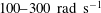
The flow after transition in a micro-channel of height approximately
 $200{-}300~\unicode[STIX]{x03BC}\text{m}$
with one soft wall (Srinivas & Kumaran Reference Srinivas and Kumaran2015) exhibits similarities and differences when compared with the turbulence in a rigid channel. The transition Reynolds number was found to be as low as 250. There is a sharp transition from a parabolic mean velocity profile to a more plug-like profile at the transition Reynolds number. The streamwise root mean square of the fluctuating velocity shows a sharp near-wall maximum, but the maximum near the soft wall is at least two times as large as that near the hard wall, suggesting that the soft wall does play a role in generating turbulence. The Reynolds stress appeared to be non-zero at the soft wall, indicating that there are velocity fluctuations in the wall material coupled to the fluid velocity fluctuations. The energy production rate was found to be a maximum at the wall itself, in contrast to the near-wall maximum due to turbulent bursting observed in a rigid channel. There was no evidence of a viscous sublayer at the soft wall to within the experimental resolution of
$200{-}300~\unicode[STIX]{x03BC}\text{m}$
with one soft wall (Srinivas & Kumaran Reference Srinivas and Kumaran2015) exhibits similarities and differences when compared with the turbulence in a rigid channel. The transition Reynolds number was found to be as low as 250. There is a sharp transition from a parabolic mean velocity profile to a more plug-like profile at the transition Reynolds number. The streamwise root mean square of the fluctuating velocity shows a sharp near-wall maximum, but the maximum near the soft wall is at least two times as large as that near the hard wall, suggesting that the soft wall does play a role in generating turbulence. The Reynolds stress appeared to be non-zero at the soft wall, indicating that there are velocity fluctuations in the wall material coupled to the fluid velocity fluctuations. The energy production rate was found to be a maximum at the wall itself, in contrast to the near-wall maximum due to turbulent bursting observed in a rigid channel. There was no evidence of a viscous sublayer at the soft wall to within the experimental resolution of
 $(yv_{\ast }/\unicode[STIX]{x1D708})\approx 2$
, where
$(yv_{\ast }/\unicode[STIX]{x1D708})\approx 2$
, where
 $y$
is the distance from the wall,
$y$
is the distance from the wall,
 $v_{\ast }$
is the friction velocity and
$v_{\ast }$
is the friction velocity and
 $\unicode[STIX]{x1D708}$
is the kinematic viscosity. A logarithmic layer was observed for
$\unicode[STIX]{x1D708}$
is the kinematic viscosity. A logarithmic layer was observed for
 $2\leqslant (yv_{\ast }/\unicode[STIX]{x1D708})\leqslant 30$
, but the von Kármán constants in the logarithmic law were found to be very different from those for the flow past a rigid surface. Wall motion was also detected by embedding beads in the wall (Verma & Kumaran Reference Verma and Kumaran2013) or by marking a spot on the wall using dye (Srinivas & Kumaran Reference Srinivas and Kumaran2015), although the frequency of the wall motion could not be determined because the Nyquist frequency for the imaging procedure used was too low.
$2\leqslant (yv_{\ast }/\unicode[STIX]{x1D708})\leqslant 30$
, but the von Kármán constants in the logarithmic law were found to be very different from those for the flow past a rigid surface. Wall motion was also detected by embedding beads in the wall (Verma & Kumaran Reference Verma and Kumaran2013) or by marking a spot on the wall using dye (Srinivas & Kumaran Reference Srinivas and Kumaran2015), although the frequency of the wall motion could not be determined because the Nyquist frequency for the imaging procedure used was too low.
The magnitudes of the velocity moments in soft-wall turbulence in the Reynolds number range of 250–400, when scaled by suitable powers of the mean velocity, were found to be comparable to those in a rigid channel at much higher Reynolds numbers, in the range 3000–20 000. Thus, the flow after transition in a soft-walled micro-channel can be characterised as turbulence, but of a different kind than that in a rigid channel, one in which wall motion plays a significant role in generating turbulent fluctuations.
1.2 Comparison with external flows
The pioneering experiments of Hansen & Hunston (Reference Hansen and Hunston1974), Hansen & Hunston (Reference Hansen and Hunston1983) and Gad-el Hak, Blackwelder & Riley (Reference Gad-el Hak, Blackwelder and Riley1985) on external flows past soft surfaces have reported the ‘static divergence’ instability, a hydroelastic instability due to the coupling between the fluid flow and a compliant surface in different experimental geometries. Hansen & Hunston (Reference Hansen and Hunston1974) considered a rotating disk geometry, where a disk coated with a compliant surface was rotated in a tank, while Hansen & Hunston (Reference Hansen and Hunston1983) examined the boundary-layer flow over a flat plate coated with a compliant material. In the case of Gad-el Hak et al. (Reference Gad-el Hak, Blackwelder and Riley1985), a flat plate partially coated with a compliant surface was towed in a tank of water. Many of the important observations in these experiments are similar, although there are some differences. All studies report the appearance of waves on the compliant surface, when the dimensionless parameter
 $V(\unicode[STIX]{x1D70C}/G)^{1/2}$
exceeds a critical value, where
$V(\unicode[STIX]{x1D70C}/G)^{1/2}$
exceeds a critical value, where
 $V$
is the free stream velocity relative to the solid surface,
$V$
is the free stream velocity relative to the solid surface,
 $G$
is the shear modulus of the compliant surface,
$G$
is the shear modulus of the compliant surface,
 $\unicode[STIX]{x1D70C}$
is the density and
$\unicode[STIX]{x1D70C}$
is the density and
 $(G/\unicode[STIX]{x1D70C})^{1/2}$
is the propagation velocity of shear waves in the solid. Hansen & Hunston (Reference Hansen and Hunston1983) reported the onset of waves on the surface both for turbulent and laminar flows. Gad-el Hak et al. (Reference Gad-el Hak, Blackwelder and Riley1985) observed an instability only for turbulent boundary-layer flows; the instability was not observed for laminar flows even when the free stream velocity was twice the shear wave velocity.
$(G/\unicode[STIX]{x1D70C})^{1/2}$
is the propagation velocity of shear waves in the solid. Hansen & Hunston (Reference Hansen and Hunston1983) reported the onset of waves on the surface both for turbulent and laminar flows. Gad-el Hak et al. (Reference Gad-el Hak, Blackwelder and Riley1985) observed an instability only for turbulent boundary-layer flows; the instability was not observed for laminar flows even when the free stream velocity was twice the shear wave velocity.
Linear stability studies of the external flows past model flexible surfaces, usually considered as spring-backed plates, have found different modes of instability. Benjamin (Reference Benjamin1960, Reference Benjamin1963), Landahl (Reference Landahl1962) classified these into three types – the class A modes which are the rigid-wall Tollmien–Schlichting instabilities modified by surface flexibility, the class B modes which have wave speed close to the surface waves on the medium and the class C or travelling wave flutter which is similar to the Kelvin–Helmholtz instability. Subsequently, Carpenter & Garrad (Reference Carpenter and Garrad1985) and Carpenter & Garrad (Reference Carpenter and Garrad1986) modified the classification to include the class B and class C modes into a category called flow-induced surface instabilities, which are qualitatively different from the Tollmien–Schlichting modes.
The characteristic features of the soft-wall instability (internal flows) and the hydroelastic instability (external flows) appear to be very different. The wall motion is primarily tangential to the surface in the internal flows and the destabilisation of the flow is due to the coupling between the mean flow and fluctuations through the tangential velocity boundary conditions at the interface. In contrast, there is the formation of surface waves and measurable normal motion in the hydroelastic instability. While viscous effects are necessary for destabilising the flow in the soft-wall instability (due to the presence of a viscous wall layer at the wall), the transition velocity for static divergence is expressed entirely in terms of the shear wave speed of the compliant wall
 $(G/\unicode[STIX]{x1D70C})^{1/2}$
, which is independent of fluid viscosity. In this sense, the static divergence instability is similar to the high Reynolds number inviscid instability theoretically predicted in the analysis of internal flows, but which does not seem to have been observed so far.
$(G/\unicode[STIX]{x1D70C})^{1/2}$
, which is independent of fluid viscosity. In this sense, the static divergence instability is similar to the high Reynolds number inviscid instability theoretically predicted in the analysis of internal flows, but which does not seem to have been observed so far.
1.3 Motivations
Based on the above summary, the motivations for the present study are as follows.
-
(i) To examine whether the soft-wall transition can be observed in turbulent flows. The pretransitional flows have always been laminar in studies carried out so far and linear stability analyses also use the laminar flow as the base state.
-
(ii) To examine whether the static divergence reported for external flows (Hansen & Hunston Reference Hansen and Hunston1974, Reference Hansen and Hunston1983; Gad-el Hak et al. Reference Gad-el Hak, Blackwelder and Riley1985) is of relevance in internal flows, since this has not been reported so far.
-
(iii) To examine the relationship between the soft-wall instability for internal flows and the hydroelastic instability for external flows. Specifically, whether the static divergence is a continuation of the soft-wall instability at high Reynolds numbers or whether the two are distinct.
-
(iv) To directly measure the profiles of the mean and fluctuating velocities after the hydroelastic instability in an internal flow, and compare these with characteristics observed after the soft-wall instability.
1.4 Outline
In order to attain Reynolds numbers of the order of a few thousands at relatively low velocities, we have used channels of higher dimensions than Verma & Kumaran (Reference Verma and Kumaran2013) and Srinivas & Kumaran (Reference Srinivas and Kumaran2015), with heights of approximately 0.6 mm and 1.8 mm. In order to decrease the value of the parameter
 $\unicode[STIX]{x1D6F4}$
, polyacrylamide gel is used, since this has a shear modulus that is an order of magnitude lower than the polydimethylsiloxane (PDMS) that was used in Verma & Kumaran (Reference Verma and Kumaran2013) and Srinivas & Kumaran (Reference Srinivas and Kumaran2015).
$\unicode[STIX]{x1D6F4}$
, polyacrylamide gel is used, since this has a shear modulus that is an order of magnitude lower than the polydimethylsiloxane (PDMS) that was used in Verma & Kumaran (Reference Verma and Kumaran2013) and Srinivas & Kumaran (Reference Srinivas and Kumaran2015).
The experimental methods are discussed in the next section, augmented by a description of the channel fabrication and gel characterisation in appendix A. The velocity measurement techniques are validated for laminar and turbulent flows in appendix B. An important issue in flow through soft channels is the effect of wall deformation. This is discussed in appendix C, where it is shown that the maximum slope of the wall is numerically small at the Reynolds numbers where transitions are observed. Due to this, the velocity profile for the laminar flow is close to the parabolic profile even in the deformed channel. The results for the transition from a laminar flow (for the gel with undeformed height 0.6 mm) and turbulent flow (for the gel with undeformed height 1.8 mm) are provided in §§ 3 and 4. Section 5 contains the important conclusions. The present results are placed in the context of previous studies, and the important open issues are discussed in § 6.
The naming convention used here is as follows. The transition in the flow through a rigid channel at a Reynolds number of approximately 1000 is called the ‘hard-wall transition’, and the flow after transition is called ‘hard-wall turbulence’. The transition and turbulence of the type observed by Verma & Kumaran (Reference Verma and Kumaran2013) and Srinivas & Kumaran (Reference Srinivas and Kumaran2015) are referred to as the ‘soft-wall transition’ and ‘soft-wall turbulence’. There is a second transition, referred to as ‘wall flutter’, which shares some of the characteristics of the hydroelastic instability of Hansen & Hunston (Reference Hansen and Hunston1974, Reference Hansen and Hunston1983) or the static divergence of Gad-el Hak et al. (Reference Gad-el Hak, Blackwelder and Riley1985). This should not be confused with the ‘aerodynamic flutter’ or ‘travelling wave flutter’ (Carpenter & Garrad Reference Carpenter and Garrad1985, Reference Carpenter and Garrad1986).
2 Experimental methods
2.1 Channel fabrication and characterisation
The channel was fabricated using polyacrylamide gel, as explained in appendix A. Three different compositions were used, resulting in gels with shear moduli 0.75 kPa, 2.19 kPa and 15.89 kPa. The gel with shear modulus 15.89 kPa is used as the hard-walled channel, since the shear modulus is sufficiently large that the soft-wall transition Reynolds number is higher than the maximum of approximately 3500 in the experiments.

Figure 1. The schematic (not to scale) of the top view (a), the cross-section of the undeformed channel (b) and the channel deformed due to a pressure gradient (c).
The channels are fabricated as a rectangular bore in a block of polyacrylamide gel with dimensions shown in figure 1. The channels consist of an upstream hard (development) section of length approximately 13 cm, made with gel of shear modulus 15.89 kPa, to damp out disturbances at the inlet. This is followed by a downstream soft section of length approximately 14 cm, where the gel has a lower elasticity modulus due to lower cross-linker concentration. The width of the channel is approximately 1.3 cm, while channels with two different heights, about 0.6 mm and 1.8 mm are fabricated. When there is a pressure difference applied across the channel, the walls deform in the test section, as shown in figure 1(c). The channel deformation is discussed in detail in appendix C.
2.2 Experimental configuration
The configuration and coordinate system used for analysing the flow are shown in figure 2. The channel is mounted on an optical breadboard with translation stages along the
 $x$
(flow) and
$x$
(flow) and
 $z$
(spanwise) directions, and goniometers with axes along the
$z$
(spanwise) directions, and goniometers with axes along the
 $x$
and
$x$
and
 $z$
axes. The inlet to the development section is connected to a pressurised tank through a needle valve for controlling the flow rate. The velocity profiles are measured using particle image velocimetry at the entrance to the test section, and it has been verified that the profiles are parabolic, as shown in appendix B.
$z$
axes. The inlet to the development section is connected to a pressurised tank through a needle valve for controlling the flow rate. The velocity profiles are measured using particle image velocimetry at the entrance to the test section, and it has been verified that the profiles are parabolic, as shown in appendix B.
The Reynolds number is defined based on the flow rate and the channel width,
 $$\begin{eqnarray}Re=\frac{\unicode[STIX]{x1D70C}Q}{W\unicode[STIX]{x1D702}},\end{eqnarray}$$
where
 $\unicode[STIX]{x1D70C}$
and
$\unicode[STIX]{x1D70C}$
and
 $\unicode[STIX]{x1D702}$
are the fluid density and viscosity,
$\unicode[STIX]{x1D702}$
are the fluid density and viscosity,
 $Q$
is the flow rate and
$Q$
is the flow rate and
 $W$
is the channel width. For a channel of rectangular cross-section the above definition reduces to that based on the average velocity and channel height. However, the definition in (2.1) is advantageous because it is independent of height, and it does not change even when there is a downstream variation in height caused by the applied pressure.
$W$
is the channel width. For a channel of rectangular cross-section the above definition reduces to that based on the average velocity and channel height. However, the definition in (2.1) is advantageous because it is independent of height, and it does not change even when there is a downstream variation in height caused by the applied pressure.
Two different configurations, shown in figure 2, are used in the experiments. In the ‘symmetric’ configuration (figure 2 a), both the top and bottom walls of the channel are fixed to glass plates. In the ‘asymmetric’ configuration (figure 2 b), the bottom wall is fixed to a glass substrate, while the top wall is unrestrained. In both cases, the soft-wall transition is observed at the same Reynolds number, to within experimental resolution. However, the ‘wall-flutter’ transition is not observed for the symmetric configuration where both walls are restrained; it is only observed for the asymmetric configuration where the top wall is unrestrained. Therefore, we report results only for the asymmetric configuration.

Figure 2. The configuration and coordinate system used for the particle image velocimetry measurements and the normal wall displacements (a) and the tangential wall displacements (b). Panel (a) also shows the symmetric configuration with a top glass plate, and panel (b) also shows the asymmetric configuration with an unrestrained top wall.
2.3 Fluid velocity measurements
The configuration shown in figure 2(a) is used to make particle image velocimetry (PIV) measurements using an IDT PIV system with a framing rate of 15 Hz. The laser sheet is directed along the centreline of the channel in the spanwise
 $z$
direction (vertical line in the cross-section figure 1
c). Glass beads with diameters in the range
$z$
direction (vertical line in the cross-section figure 1
c). Glass beads with diameters in the range
 $8{-}14~\unicode[STIX]{x03BC}\text{m}$
were used for seeding the flow.
$8{-}14~\unicode[STIX]{x03BC}\text{m}$
were used for seeding the flow.
The PIV measurements are carried out at four different downstream locations, I, II, III and IV, shown in figure 1(a). There is very little variation in the velocity statistics between downstream locations III and IV. The PIV measurements for both laminar and turbulent flows are validated in appendix B.
For each channel configuration (wall shear modulus and height) and at each Reynolds number, two independent sequences of 2000 pairs of images each are recorded. These are separated into eight subsequences of 500 image pairs each. The mean value of a velocity moment is the average over the entire 4000 pairs of images. Eight averages over subsequences of 500 image pairs each are determined, and the standard deviation is calculated for these eight measurements. The error bars in the experimental results show one standard deviation above and below the mean value.
It is important to note that due to the size of the particles, it is not possible to determine the velocity within a distance of approximately
 $15~\unicode[STIX]{x03BC}\text{m}$
from the wall. Therefore, in most of the profiles for the fluctuating velocities and Reynolds stress, the results are not shown within a distance of approximately
$15~\unicode[STIX]{x03BC}\text{m}$
from the wall. Therefore, in most of the profiles for the fluctuating velocities and Reynolds stress, the results are not shown within a distance of approximately
 $20~\unicode[STIX]{x03BC}\text{m}$
from the wall. In cases such as the mean velocity profile, where the results are shown at the wall, these results are extrapolated.
$20~\unicode[STIX]{x03BC}\text{m}$
from the wall. In cases such as the mean velocity profile, where the results are shown at the wall, these results are extrapolated.
The particle size is approximately 3 % of the channel height for the smaller channel and approximately 1 % of the channel height for the larger channel. The uncertainties in the fluid velocity measurements due to the finite size of the particles can be estimated as follows.
-
(i) The particle size, approximately
 $10~\unicode[STIX]{x03BC}\text{m}$
, is much smaller than the two channel heights of 0.6 mm and 1.8 mm considered here. However, the smallest scales in a turbulent flow could be much smaller than the channel height. If we consider the Kolmogorov estimate for the smallest length scale as
$Re^{-3/4}h$
, the smallest scale in a channel of height 0.6 mm at a maximum Reynolds number of approximately 900 is approximately
$3.6~\unicode[STIX]{x03BC}\text{m}$
, and for a channel of height 1.8 mm at a maximum Reynolds number of 2500 is approximately
$5.1~\unicode[STIX]{x03BC}\text{m}$
. (The Kolmogorov estimate is an underestimate for the low Reynolds numbers used here.) Thus, the particle diameter is 2–3 times larger than the smallest scales. Although the particle trajectories may not accurately capture the smallest scales, they most certainly capture the large-scale structures in the flow.
$10~\unicode[STIX]{x03BC}\text{m}$
, is much smaller than the two channel heights of 0.6 mm and 1.8 mm considered here. However, the smallest scales in a turbulent flow could be much smaller than the channel height. If we consider the Kolmogorov estimate for the smallest length scale as
$Re^{-3/4}h$
, the smallest scale in a channel of height 0.6 mm at a maximum Reynolds number of approximately 900 is approximately
$3.6~\unicode[STIX]{x03BC}\text{m}$
, and for a channel of height 1.8 mm at a maximum Reynolds number of 2500 is approximately
$5.1~\unicode[STIX]{x03BC}\text{m}$
. (The Kolmogorov estimate is an underestimate for the low Reynolds numbers used here.) Thus, the particle diameter is 2–3 times larger than the smallest scales. Although the particle trajectories may not accurately capture the smallest scales, they most certainly capture the large-scale structures in the flow. -
(ii) The effect of fluid inertia on the particle trajectories can be estimated from the particle Reynolds number based on the fluid fluctuating velocity,
$(\unicode[STIX]{x1D70C}d_{p}v^{\prime }/\unicode[STIX]{x1D702})$
where
$d_{p}$
is the particle diameter and
$v^{\prime }$
is the fluid fluctuating velocity. (Here, the fluctuating velocity has been used as the basis for calculating inertial effects, because the particle mean velocity relaxes to the local fluid mean velocity within a time period estimated in the item (iii).) For the channel with height about 0.6 mm, the maximum of the streamwise fluctuating velocity are about
$0.07~\text{m}~\text{s}^{-1}$
at the soft-wall transition and
$0.3~\text{m}~\text{s}^{-1}$
at the wall-flutter transition, and the corresponding Reynolds numbers are 0.7 and 3 respectively. For the channel with height approximately 1.8 mm, the maximum of the streamwise fluctuating velocity is approximately 0.06 at the soft-wall transition and approximately 0.15 at the wall-flutter transition, and the corresponding Reynolds numbers are approximately 0.6 and 1.5 for
$10~\unicode[STIX]{x03BC}\text{m}$
particles. When the particle Reynolds number is less than 3, there is no separation or formation of closed streamlines at the rear of the sphere, and the drag force exceeds the Stokes drag law by approximately 20 %. -
(iii) The fidelity with which the particles follow streamlines depends on the particle Stokes number, which is the ratio of the viscous relaxation time of the particle and the fluid integral time scale. Based on Stokes drag law, the viscous relaxation time of the particle,
$\unicode[STIX]{x1D70F}_{v}=(m/3\unicode[STIX]{x03C0}\unicode[STIX]{x1D707}d_{p})$
, is
$4.3\times 10^{-5}~\text{s}$
for glass spheres with density
$2500~\text{kg}~\text{m}^{-3}$
and diameter
$10~\unicode[STIX]{x03BC}\text{m}$
. The fluid integral time scales as the inverse of the macroscopic strain rate,
$(h/\bar{v}_{x})$
, where
$h$
is the channel height and
$\bar{v}_{x}$
is the mean velocity. Based on the maximum velocity of
$2~\text{m}~\text{s}^{-1}$
for the channel of height 0.6 mm and
$1.4~\text{m}~\text{s}^{-1}$
for the channel of height 1.8 mm, the fluid time scales for the largest eddies are
$\unicode[STIX]{x1D70F}_{I}=3\times 10^{-4}~\text{s}$
(approximately
$7\unicode[STIX]{x1D70F}_{p}$
) for the smaller channel and
$1.3\times 10^{-3}$
s (approximately
$30\unicode[STIX]{x1D70F}_{p}$
) for the larger channel. Both of these are much larger than the particle relaxation time. The turnover times for the smallest eddies in the flow are, of course, much smaller than those for the large-scale structures. If we use the Kolmogorov estimate, the time scales for the smallest eddies are
$Re^{-1/2}$
smaller than the large-scale flow. (The Kolmogorov time scale underpredicts the smallest relaxation time for low Reynolds numbers up to approximately 2500 used here.) For a the channels of height 0.6 mm, the maximum Reynolds number is approximately 900, and so the smallest eddy turnover time is about 30 times smaller than that for the largest eddies, which is about
$0.25\unicode[STIX]{x1D70F}_{p}$
. For the larger channels of height 1.8 mm, the maximum Reynolds number is approximately 2500, and so the smallest eddy turnover time is about 50 times smaller than that for the largest eddies, which is about
$0.6\unicode[STIX]{x1D70F}_{p}$
. Thus, the particle relaxation time is somewhat larger than the Kolmogorov estimate of the smallest eddy turnover time by a factor of 2–4, but is certainly much smaller than the turnover time of the largest eddies. -
(iv) Close to the wall, a lift force could be generated due to the particle rotation and the particle motion relative to the wall. The Magnus lift force on the particles scales as
$C_{L}((\unicode[STIX]{x03C0}/8)\unicode[STIX]{x1D70C}v_{p}(\bar{v}_{x}d_{p}^{2}))$
, where
$v_{p}$
is the particle velocity relative to the fluid,
$\bar{v}_{x}d_{p}^{2}$
is a measure of the circulation of the fluid around the particle due to the mean flow and
$C_{L}$
is the lift coefficient. If we consider the fluid fluctuating velocity
$v^{\prime }$
as the characteristic particle velocity, the lift force is
$C_{L}((\unicode[STIX]{x03C0}/8)\unicode[STIX]{x1D70C}\bar{v}_{x}v^{\prime }d_{p}^{2})$
. The ratio of the lift and the drag force
$3\unicode[STIX]{x03C0}\unicode[STIX]{x1D707}d_{p}v^{\prime }$
is,
$(C_{L}\unicode[STIX]{x1D70C}\bar{v}_{x}d_{p}^{2}/24\unicode[STIX]{x1D707}h)\sim (C_{L}Re(d_{p}/h)^{2}/24)$
, where
$Re$
is the Reynolds number based on the mean velocity. Zang, Balachandar & Fisher (Reference Zang, Balachandar and Fisher2005) report that
$C_{L}$
is in the range
$0.1{-}1.1$
when the distance of the particle centre from the wall is
$0.75d_{p}$
to
$d_{p}$
, and when the particle Reynolds number is less than 10. For the channel with height 0.6 mm and a maximum Reynolds number of approximately 900, this ratio of the lift and drag forces is approximately 0.01, while for the channel with height approximately 1.8 mm at a maximum Reynolds number of approximately 2500, this ratio is approximately 0.003. Thus, the lift force is likely to be much smaller than the correction to the drag force due to inertial effects.


2.4 Wall displacement measurements
The normal and tangential wall displacement in the soft wall were also measured by embedding glass beads of diameter
 $8{-}14~\unicode[STIX]{x03BC}\text{m}$
within the wall during the fabrication process. The glass beads were mixed into the prepolymer before gelation, and they were rigidly fixed in the solid due to the formation of cross-links in the polymer after gelation. A camera connected to a zoom tube was used to record the displacement of a bead close to the surface. The displacement was determined from the correlation peak in the Fourier transform of the grey scale intensity matrix, as discussed in Srinivas & Kumaran (Reference Srinivas and Kumaran2015). In order to determine the tangential displacement of the wall in the
$8{-}14~\unicode[STIX]{x03BC}\text{m}$
within the wall during the fabrication process. The glass beads were mixed into the prepolymer before gelation, and they were rigidly fixed in the solid due to the formation of cross-links in the polymer after gelation. A camera connected to a zoom tube was used to record the displacement of a bead close to the surface. The displacement was determined from the correlation peak in the Fourier transform of the grey scale intensity matrix, as discussed in Srinivas & Kumaran (Reference Srinivas and Kumaran2015). In order to determine the tangential displacement of the wall in the
 $x$
and
$x$
and
 $z$
directions, the configuration in figure 2(b) was used, and images of the beads at both the top and bottom surfaces were captured. Due to the clear line of view from above, relatively high magnification was achieved for the tangential displacement of the surface – an area of dimension 0.375 mm
$z$
directions, the configuration in figure 2(b) was used, and images of the beads at both the top and bottom surfaces were captured. Due to the clear line of view from above, relatively high magnification was achieved for the tangential displacement of the surface – an area of dimension 0.375 mm
 $\times$
0.222 mm was imaged with a resolution of 804
$\times$
0.222 mm was imaged with a resolution of 804
 $\times$
484 pixels, resulting in each pixel occupying a linear dimension of approximately
$\times$
484 pixels, resulting in each pixel occupying a linear dimension of approximately
 $0.466~\unicode[STIX]{x03BC}\text{m}$
. For the normal wall displacement in the
$0.466~\unicode[STIX]{x03BC}\text{m}$
. For the normal wall displacement in the
 $y$
direction, the configuration in figure 2(a) was used, where images of an embedded bead is captured from the side. In this case, the magnification achieved was relatively less due to the relatively large depth of view required, as indicated in the cross-section in figure 1(b,c). An area of 7 mm
$y$
direction, the configuration in figure 2(a) was used, where images of an embedded bead is captured from the side. In this case, the magnification achieved was relatively less due to the relatively large depth of view required, as indicated in the cross-section in figure 1(b,c). An area of 7 mm
 $\times$
4.24 mm was imaged with a resolution of 804
$\times$
4.24 mm was imaged with a resolution of 804
 $\times$
484 pixel, resulting in each pixel occupying a linear dimension of approximately
$\times$
484 pixel, resulting in each pixel occupying a linear dimension of approximately
 $8.7~\unicode[STIX]{x03BC}\text{m}$
.
$8.7~\unicode[STIX]{x03BC}\text{m}$
.
The spectra of the displacement fields were determined by taking the Fourier transform of the time series of the displacement data,
 $$\begin{eqnarray}\displaystyle \tilde{\star }(\unicode[STIX]{x1D714})=\frac{1}{T}\int _{0}^{T}\,\text{d}t\exp (\imath \unicode[STIX]{x1D714}t)\star (t), & & \displaystyle\end{eqnarray}$$
where
 $\star (t)$
is the time series of the relevant component of the displacement of a bead embedded in the wall. In our experiments, the maximum framing rate is 1000 Hz, and consequently the Nyquist frequency is 500 Hz. Since oversampling by a factor of 5–10 is required for accurately capturing the spectra, the maximum frequency reported here is approximately
$\star (t)$
is the time series of the relevant component of the displacement of a bead embedded in the wall. In our experiments, the maximum framing rate is 1000 Hz, and consequently the Nyquist frequency is 500 Hz. Since oversampling by a factor of 5–10 is required for accurately capturing the spectra, the maximum frequency reported here is approximately
 $500~\text{rad}~\text{s}^{-1}$
. The time period
$500~\text{rad}~\text{s}^{-1}$
. The time period
 $T$
used was usually 1 s, although longer sequences of up to 15 s were used to verify that there are no systematic low-frequency signals. The frequency spectrum is calculated only for the tangential displacement recorded from above as shown in figure 1(b), because the resolution is much higher than that for the normal displacement recorded from the side as shown in figure 1(a).
$T$
used was usually 1 s, although longer sequences of up to 15 s were used to verify that there are no systematic low-frequency signals. The frequency spectrum is calculated only for the tangential displacement recorded from above as shown in figure 1(b), because the resolution is much higher than that for the normal displacement recorded from the side as shown in figure 1(a).
For the wall displacement measurements, three sequences of 1000 frames (1 second) each are recorded. The average and the root mean square of the displacement are calculated as averages over all three sequences (3000 frames). The averages for each subsequence of 1000 frames is also calculated, and the standard deviation is determined using the averages for the three subsequences.
3 Transitions from a laminar flow
The flow in a channel of height 0.6 mm is considered, where the soft-wall and wall-flutter transitions take place at Reynolds numbers less than 1000 for transition in a rigid channel. The results for the flow characteristics and the wall dynamics after the soft-wall transition are analysed in § 3.1, followed by the results for the flow after the wall-flutter transition in § 3.2.
3.1 Soft-wall transition
3.1.1 Flow characteristics
The mean velocity profiles across the channel with walls made of shear modulus 0.75 kPa at the downstream location III (figure 1
a) are shown in figure 3. The bottom wall of the channel is at
 $y=0$
, while the location of the top wall is shown by the dashed vertical lines on the right in figure 3. The height increase is quite small at the downstream location III at Reynolds numbers up to 500 – the height increases by only 8 % when the Reynolds number increases from 278 to 448. However, the qualitative features reported here are also observed at the other locations.
$y=0$
, while the location of the top wall is shown by the dashed vertical lines on the right in figure 3. The height increase is quite small at the downstream location III at Reynolds numbers up to 500 – the height increases by only 8 % when the Reynolds number increases from 278 to 448. However, the qualitative features reported here are also observed at the other locations.

Figure 3. The cross-stream variation of
 $\bar{v}_{x}$
(a);
$\bar{v}_{x}$
(a);
 $v_{x}^{\prime }$
(b);
$v_{x}^{\prime }$
(b);
 $v_{y}^{\prime }$
(c);
$v_{y}^{\prime }$
(c);
 $\langle v_{x}^{\prime }v_{y}^{\prime }\rangle$
(d); the stress
$\langle v_{x}^{\prime }v_{y}^{\prime }\rangle$
(d); the stress
 $\unicode[STIX]{x1D70F}_{xy}$
(solid line) and viscous stress
$\unicode[STIX]{x1D70F}_{xy}$
(solid line) and viscous stress
 $\unicode[STIX]{x1D70F}_{xy}^{v}$
(red dashed line) (e); and
$\unicode[STIX]{x1D70F}_{xy}^{v}$
(red dashed line) (e); and
 $(\bar{v}_{x}/v_{\ast })$
versus
$(\bar{v}_{x}/v_{\ast })$
versus
 $(yv_{\ast }/\unicode[STIX]{x1D708})$
(f), at location III (figure 1
a) when the wall is made of shear modulus 0.75 kPa at Reynolds number
$(yv_{\ast }/\unicode[STIX]{x1D708})$
(f), at location III (figure 1
a) when the wall is made of shear modulus 0.75 kPa at Reynolds number
 $278$
(○),
$278$
(○),
 $301$
(▵),
$301$
(▵),
 $335$
(▿),
$335$
(▿),
 $392$
(◃) and
$392$
(◃) and
 $448$
(▹) for a channel with height approximately 0.6 mm in the undeformed state. The vertical dashed lines show the location of the top wall and the dashed curves in panel (a) show parabolic velocity profiles with equal average velocity. In panel (f), the dotted curve is
$448$
(▹) for a channel with height approximately 0.6 mm in the undeformed state. The vertical dashed lines show the location of the top wall and the dashed curves in panel (a) show parabolic velocity profiles with equal average velocity. In panel (f), the dotted curve is
 $(\bar{v}_{x}/v_{\ast })=(yv_{\ast }/\unicode[STIX]{x1D708})$
, and the dashed line is
$(\bar{v}_{x}/v_{\ast })=(yv_{\ast }/\unicode[STIX]{x1D708})$
, and the dashed line is
 $(\bar{v}_{x}/v_{\ast })=3.45(yv_{\ast }/\unicode[STIX]{x1D708})-1.8$
.
$(\bar{v}_{x}/v_{\ast })=3.45(yv_{\ast }/\unicode[STIX]{x1D708})-1.8$
.
In figure 3(a), the dashed curves show the parabolic profiles that have the same average velocity as the experimentally measured profiles. It is observed that the velocity profiles are parabolic up to a Reynolds number of 301. When the Reynolds number increases to 335, there is a distinct departure from the parabolic profile, and the difference is significantly higher than the experimental standard deviation. The experimental velocity profiles are clearly flatter at the centre and steeper at the walls in comparison to the parabolic profile. At
 $Re=335$
, the root mean square of the streamwise fluctuating velocity
$Re=335$
, the root mean square of the streamwise fluctuating velocity
 $v_{x}^{\prime }$
shows a significant increase in magnitude (figure 3
b). More importantly, the shape of the
$v_{x}^{\prime }$
shows a significant increase in magnitude (figure 3
b). More importantly, the shape of the
 $v_{x}^{\prime }$
profile exhibits the near-wall maxima which are characteristic of a turbulent flow in a channel. A significant increase in the cross-stream root mean square velocity,
$v_{x}^{\prime }$
profile exhibits the near-wall maxima which are characteristic of a turbulent flow in a channel. A significant increase in the cross-stream root mean square velocity,
 $v_{y}^{\prime }$
is also observed in figure 3(c) when the Reynolds number increases from
$v_{y}^{\prime }$
is also observed in figure 3(c) when the Reynolds number increases from
 $301$
to
$301$
to
 $335$
. Figure 3(d) shows that the correlation
$335$
. Figure 3(d) shows that the correlation
 $\langle v_{x}^{\prime }v_{y}^{\prime }\rangle$
, which is zero to within the experimental standard deviation for
$\langle v_{x}^{\prime }v_{y}^{\prime }\rangle$
, which is zero to within the experimental standard deviation for
 $Re\leqslant 301$
, increases significantly in magnitude at
$Re\leqslant 301$
, increases significantly in magnitude at
 $Re=337$
and exhibits the characteristic shape of the Reynolds stress profiles in channel flow.
$Re=337$
and exhibits the characteristic shape of the Reynolds stress profiles in channel flow.
Subject to experimental uncertainties, the mean velocity and the root mean square of the fluctuating velocities are symmetric, and
 $\langle v_{x}^{\prime }v_{y}^{\prime }\rangle$
is antisymmetric, about the centreline of the channel. The transition at the Reynolds number of
$\langle v_{x}^{\prime }v_{y}^{\prime }\rangle$
is antisymmetric, about the centreline of the channel. The transition at the Reynolds number of
 $335$
is also significantly different from those for a rigid channel in some important aspects. Due to experimental limitations (the seed particles are
$335$
is also significantly different from those for a rigid channel in some important aspects. Due to experimental limitations (the seed particles are
 $8{-}14~\unicode[STIX]{x03BC}\text{m}$
in diameter), it is not possible to resolve the region within a distance of
$8{-}14~\unicode[STIX]{x03BC}\text{m}$
in diameter), it is not possible to resolve the region within a distance of
 $15~\unicode[STIX]{x03BC}\text{m}$
from the wall of the channel. The data in figures 3(b) and 3(c) suggest that the root mean square of the fluctuating velocities could be non-zero at both walls although the data could plausibly be extrapolated to zero velocity at the wall. The data in figure 3(d) do suggest that
$15~\unicode[STIX]{x03BC}\text{m}$
from the wall of the channel. The data in figures 3(b) and 3(c) suggest that the root mean square of the fluctuating velocities could be non-zero at both walls although the data could plausibly be extrapolated to zero velocity at the wall. The data in figure 3(d) do suggest that
 $\langle v_{x}^{\prime }v_{y}^{\prime }\rangle$
is non-zero at both walls. It should be noted that there are uncertainties in the measurement of the fluctuating velocities close to the wall. However, figure 21(c) in appendix B for a Reynolds number of approximately 3500 indicates that it is possible to capture the Reynolds stress accurately within approximately
$\langle v_{x}^{\prime }v_{y}^{\prime }\rangle$
is non-zero at both walls. It should be noted that there are uncertainties in the measurement of the fluctuating velocities close to the wall. However, figure 21(c) in appendix B for a Reynolds number of approximately 3500 indicates that it is possible to capture the Reynolds stress accurately within approximately
 $50~\unicode[STIX]{x03BC}\text{m}$
of the wall, and a steep decrease in the Reynolds stress is observed at the wall. In contrast, in figure 3(d), a reasonable polynomial extrapolation predicts a non-zero Reynolds stress at the wall, although a sharp decrease in the Reynolds stress close to the wall cannot be ruled out by our measurements. More work is required to resolve this issue.
$50~\unicode[STIX]{x03BC}\text{m}$
of the wall, and a steep decrease in the Reynolds stress is observed at the wall. In contrast, in figure 3(d), a reasonable polynomial extrapolation predicts a non-zero Reynolds stress at the wall, although a sharp decrease in the Reynolds stress close to the wall cannot be ruled out by our measurements. More work is required to resolve this issue.
Figure 3(e) shows the variation in the total stress
 $$\begin{eqnarray}\unicode[STIX]{x1D70F}_{xy}=\unicode[STIX]{x1D702}(\text{d}\bar{v}_{x}/\text{d}y)-\unicode[STIX]{x1D70C}\langle v_{x}^{\prime }v_{y}^{\prime }\rangle ,\end{eqnarray}$$
as well as the variation in the viscous stress
 $\unicode[STIX]{x1D70F}_{xy}^{v}=\unicode[STIX]{x1D702}(\text{d}\bar{v}_{x}/\text{d}y)$
, as a function of the cross-stream distance. For
$\unicode[STIX]{x1D70F}_{xy}^{v}=\unicode[STIX]{x1D702}(\text{d}\bar{v}_{x}/\text{d}y)$
, as a function of the cross-stream distance. For
 $Re\leqslant 301$
, the viscous stress is a linear function of distance (because the mean velocity profile is parabolic), and the difference between the total and viscous stress is smaller than the experimental uncertainty in the stress measurement. However, for
$Re\leqslant 301$
, the viscous stress is a linear function of distance (because the mean velocity profile is parabolic), and the difference between the total and viscous stress is smaller than the experimental uncertainty in the stress measurement. However, for
 $Re\geqslant 335$
, there is a significant difference between the viscous and the total stress, indicating that the Reynolds stress provides a substantial contribution to the total stress, even at the wall of the channel. Moreover, the viscous stress profiles are not a linear function of the cross-stream distance. The total stress profiles are expected to be nearly linear, since the wall slope is small at the location III (figure 1
a), as shown in figure 23 in appendix C. The linear stress profile can be obtained only when the Reynolds stress (which is non-zero at the wall) is added to the viscous stress, suggesting that the fluctuating velocities play an important role in the cross-stream transport of momentum.
$Re\geqslant 335$
, there is a significant difference between the viscous and the total stress, indicating that the Reynolds stress provides a substantial contribution to the total stress, even at the wall of the channel. Moreover, the viscous stress profiles are not a linear function of the cross-stream distance. The total stress profiles are expected to be nearly linear, since the wall slope is small at the location III (figure 1
a), as shown in figure 23 in appendix C. The linear stress profile can be obtained only when the Reynolds stress (which is non-zero at the wall) is added to the viscous stress, suggesting that the fluctuating velocities play an important role in the cross-stream transport of momentum.
The near-wall variation in the mean velocity
 $\bar{v}_{x}$
, scaled by the friction velocity
$\bar{v}_{x}$
, scaled by the friction velocity
 $v_{\ast }=(\unicode[STIX]{x1D70F}_{w}/\unicode[STIX]{x1D70C})^{1/2}$
, is shown as a function of the scaled distance
$v_{\ast }=(\unicode[STIX]{x1D70F}_{w}/\unicode[STIX]{x1D70C})^{1/2}$
, is shown as a function of the scaled distance
 $yv_{\ast }/\unicode[STIX]{x1D708}$
in figure 3(f). Here,
$yv_{\ast }/\unicode[STIX]{x1D708}$
in figure 3(f). Here,
 $\unicode[STIX]{x1D70F}_{w}$
is the wall shear stress which is the sum of the viscous stress and the Reynolds stress at the wall and
$\unicode[STIX]{x1D70F}_{w}$
is the wall shear stress which is the sum of the viscous stress and the Reynolds stress at the wall and
 $\unicode[STIX]{x1D708}$
is the kinematic viscosity. The velocity profile satisfies the linear relationship
$\unicode[STIX]{x1D708}$
is the kinematic viscosity. The velocity profile satisfies the linear relationship
 $(\bar{v}_{x}/v_{\ast })=(yv_{\ast }/\unicode[STIX]{x1D708})$
close to the wall for the laminar profile for
$(\bar{v}_{x}/v_{\ast })=(yv_{\ast }/\unicode[STIX]{x1D708})$
close to the wall for the laminar profile for
 $Re\leqslant 301$
. In the turbulent regime for
$Re\leqslant 301$
. In the turbulent regime for
 $335\leqslant Re\leqslant 448$
, there is no evidence of a viscous sublayer to within the experimental resolution for
$335\leqslant Re\leqslant 448$
, there is no evidence of a viscous sublayer to within the experimental resolution for
 $(yv_{\ast }/\unicode[STIX]{x1D708})\leqslant 2$
. However, in the narrow range
$(yv_{\ast }/\unicode[STIX]{x1D708})\leqslant 2$
. However, in the narrow range
 $3\leqslant (yv_{\ast }/\unicode[STIX]{x1D708})\leqslant 20$
, there is clear evidence of a logarithmic layer,
$3\leqslant (yv_{\ast }/\unicode[STIX]{x1D708})\leqslant 20$
, there is clear evidence of a logarithmic layer,
 $(\bar{v}_{x}/v_{\ast })=A\log (yv_{\ast }/\unicode[STIX]{x1D708})+B$
, at both the top and bottom walls.
$(\bar{v}_{x}/v_{\ast })=A\log (yv_{\ast }/\unicode[STIX]{x1D708})+B$
, at both the top and bottom walls.
The von Kármán plots for the mean velocity are shown in more detail in figure 4 at different downstream locations when the walls are made of shear modulus 0.75 kPa and 2.19 kPa, only for the Reynolds numbers where soft-wall turbulence is observed. It is clear that all the velocity profiles, scaled by the friction velocity, do follow a logarithmic law for
 $3\leqslant (yv_{\ast }/\unicode[STIX]{x1D708})\leqslant 20$
. There is no visible viscous sublayer observed even for
$3\leqslant (yv_{\ast }/\unicode[STIX]{x1D708})\leqslant 20$
. There is no visible viscous sublayer observed even for
 $(yv_{\ast }/\unicode[STIX]{x1D708})$
as low as
$(yv_{\ast }/\unicode[STIX]{x1D708})$
as low as
 $1$
. The best fits for the von Kármán constants do change when the shear modulus is changed, and the constants are also very different from those in the turbulent flow past a rigid surface.
$1$
. The best fits for the von Kármán constants do change when the shear modulus is changed, and the constants are also very different from those in the turbulent flow past a rigid surface.

Figure 4. The near-wall velocity profiles when the wall is made of shear modulus 0.75 kPa (a) and 2.19 kPa (b) for a channel with height about 0.6 mm in the undeformed state. In panel (a), ○ location II,
 $Re=340$
; ▵ location II,
$Re=340$
; ▵ location II,
 $Re=441$
; ▿ location II,
$Re=441$
; ▿ location II,
 $Re=539$
; ◃ location III,
$Re=539$
; ◃ location III,
 $Re=335$
; ▹ location III,
$Re=335$
; ▹ location III,
 $Re=392$
; ♢ location III,
$Re=392$
; ♢ location III,
 $Re=448$
;
$Re=448$
;
 $\times$
location IV,
$\times$
location IV,
 $Re=335$
;
$Re=335$
;
 $+$
location IV,
$+$
location IV,
 $Re=467$
, the dotted curve shows the relation
$Re=467$
, the dotted curve shows the relation
 $(\bar{v}_{x}/v_{\ast })=(yv_{\ast }/\unicode[STIX]{x1D708})$
; and the dashed line shows the relation
$(\bar{v}_{x}/v_{\ast })=(yv_{\ast }/\unicode[STIX]{x1D708})$
; and the dashed line shows the relation
 $(\bar{v}_{x}/v_{\ast })=3.45\log (yv_{\ast }/\unicode[STIX]{x1D708})-1.8$
. In panel (b), ○ location II,
$(\bar{v}_{x}/v_{\ast })=3.45\log (yv_{\ast }/\unicode[STIX]{x1D708})-1.8$
. In panel (b), ○ location II,
 $Re=599$
; ▵ location II,
$Re=599$
; ▵ location II,
 $Re=668$
; ▿ location II,
$Re=668$
; ▿ location II,
 $Re=758$
; ◃ location III,
$Re=758$
; ◃ location III,
 $Re=600$
; ▹ location III,
$Re=600$
; ▹ location III,
 $Re=674$
; ♢ location III,
$Re=674$
; ♢ location III,
 $Re=757$
;
$Re=757$
;
 $\times$
location IV,
$\times$
location IV,
 $Re=599$
;
$Re=599$
;
 $+$
location IV,
$+$
location IV,
 $Re=665$
; ● location IV,
$Re=665$
; ● location IV,
 $Re=779$
; the dotted curve is
$Re=779$
; the dotted curve is
 $(\bar{v}_{x}/v_{\ast })=(yv_{\ast }/\unicode[STIX]{x1D708})$
; and the dashed line is
$(\bar{v}_{x}/v_{\ast })=(yv_{\ast }/\unicode[STIX]{x1D708})$
; and the dashed line is
 $(\bar{v}_{x}/v_{\ast })=3.67\log (yv_{\ast }/\unicode[STIX]{x1D708})-2.53$
.
$(\bar{v}_{x}/v_{\ast })=3.67\log (yv_{\ast }/\unicode[STIX]{x1D708})-2.53$
.

Figure 5. The measures
 $\bar{v}_{diff}$
(a)
$\bar{v}_{diff}$
(a)
 $(\max (v_{x}^{\prime })/\bar{v})$
(b),
$(\max (v_{x}^{\prime })/\bar{v})$
(b),
 $(\max (v_{y}^{\prime })/\bar{v})$
(c) and
$(\max (v_{y}^{\prime })/\bar{v})$
(c) and
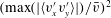 $(\max (|\langle v_{x}^{\prime }v_{y}^{\prime }\rangle |)/\bar{v})^{2}$
(d), as a function of the Reynolds number for a channel with height about 0.6 mm in the undeformed state at locations II (○), III (▵) and IV (▿) shown in figure 1(a), when the channel is made of gel of shear modulus 0.75 kPa (solid line) and 2.19 kPa (dashed line). The symbol ♢ shows the respective measures for the flow in a rigid channel. The Reynolds number for the soft-wall and wall-flutter transitions are shown using the labels SW and WF respectively.
$(\max (|\langle v_{x}^{\prime }v_{y}^{\prime }\rangle |)/\bar{v})^{2}$
(d), as a function of the Reynolds number for a channel with height about 0.6 mm in the undeformed state at locations II (○), III (▵) and IV (▿) shown in figure 1(a), when the channel is made of gel of shear modulus 0.75 kPa (solid line) and 2.19 kPa (dashed line). The symbol ♢ shows the respective measures for the flow in a rigid channel. The Reynolds number for the soft-wall and wall-flutter transitions are shown using the labels SW and WF respectively.
Quantitative measures of the departure from the parabolic profile and the velocity fluctuations, shown in figure 5, are now analysed. A quantitative measure of the difference between the actual profile and the parabolic velocity profile is,
 $$\begin{eqnarray}\displaystyle \bar{v}_{diff}=\sqrt{\frac{1}{h(\bar{v}_{x}^{(p)})^{2}}\int _{0}^{h}\,\text{d}y(\bar{v}_{x}(y)-\bar{v}_{x}^{l}(y))^{2}}, & & \displaystyle\end{eqnarray}$$
where
 $\bar{v}_{x}^{(p)}$
is the profile-averaged mean velocity defined in (C 1) and
$\bar{v}_{x}^{(p)}$
is the profile-averaged mean velocity defined in (C 1) and
 $\bar{v}_{x}^{l}(y)$
is the parabolic profile with average velocity equal to
$\bar{v}_{x}^{l}(y)$
is the parabolic profile with average velocity equal to
 $\bar{v}_{x}^{(p)}$
. The other measures used are the scaled maxima of the root mean square velocity fluctuations,
$\bar{v}_{x}^{(p)}$
. The other measures used are the scaled maxima of the root mean square velocity fluctuations,
 $\max (v_{x}^{\prime })/\bar{v}$
and
$\max (v_{x}^{\prime })/\bar{v}$
and
 $\max (v_{y}^{\prime })/\bar{v}$
, and the maximum of
$\max (v_{y}^{\prime })/\bar{v}$
, and the maximum of
 $|\langle v_{x}^{\prime }v_{y}^{\prime }\rangle |/\bar{v}^{2}$
, where
$|\langle v_{x}^{\prime }v_{y}^{\prime }\rangle |/\bar{v}^{2}$
, where
 $\bar{v}$
is the average velocity (ratio of the flow rate and the channel cross-section).
$\bar{v}$
is the average velocity (ratio of the flow rate and the channel cross-section).
The measure
 $\bar{v}_{diff}$
is shown as a function of Reynolds number in figure 5(a). There is relatively little variation in
$\bar{v}_{diff}$
is shown as a function of Reynolds number in figure 5(a). There is relatively little variation in
 $\bar{v}_{diff}$
downstream of location III, indicating that the flow has reached a fully developed state downstream of location III (figure 1
a). There is a sharp increase in
$\bar{v}_{diff}$
downstream of location III, indicating that the flow has reached a fully developed state downstream of location III (figure 1
a). There is a sharp increase in
 $\bar{v}_{diff}$
at a Reynolds number of approximately 335 when the shear modulus of the walls is 0.75 kPa, and at approximately 480 in the shear modulus of the walls is 2.19 kPa. The increase in
$\bar{v}_{diff}$
at a Reynolds number of approximately 335 when the shear modulus of the walls is 0.75 kPa, and at approximately 480 in the shear modulus of the walls is 2.19 kPa. The increase in
 $\bar{v}_{diff}$
takes place at the same Reynolds number as the steep increase in the maximum values of
$\bar{v}_{diff}$
takes place at the same Reynolds number as the steep increase in the maximum values of
 $v_{x}^{\prime }$
,
$v_{x}^{\prime }$
,
 $v_{y}^{\prime }$
and
$v_{y}^{\prime }$
and
 $\langle v_{x}^{\prime }v_{y}^{\prime }\rangle$
in figure 5(b–d). This Reynolds number is labelled as SW (for soft-wall transition) in figure 5. The root mean square of the fluctuating velocities in the streamwise and cross-stream directions initially increase rapidly when the transition Reynolds number is exceeded, and then saturate at approximately 12 % and 8 % of the mean velocity for soft-wall turbulence. Despite the sharp nature of the transition, we did not detect any hysteresis in the transition Reynolds number while increasing and decreasing the flow velocity, suggesting that this transition is supercritical.
$\langle v_{x}^{\prime }v_{y}^{\prime }\rangle$
in figure 5(b–d). This Reynolds number is labelled as SW (for soft-wall transition) in figure 5. The root mean square of the fluctuating velocities in the streamwise and cross-stream directions initially increase rapidly when the transition Reynolds number is exceeded, and then saturate at approximately 12 % and 8 % of the mean velocity for soft-wall turbulence. Despite the sharp nature of the transition, we did not detect any hysteresis in the transition Reynolds number while increasing and decreasing the flow velocity, suggesting that this transition is supercritical.
An important observation in figure 5 is that the magnitudes of the turbulent velocity fluctuations (when scaled by suitable powers of the average velocity) after the soft-wall transition are significantly higher than those observed at the hard-wall transition at a Reynolds number of approximately 1000 in a rigid channel shown by the ♢ symbols.
3.1.2 Wall dynamics
The mean displacement of the top and bottom walls in the streamwise
 $(x)$
direction are shown as a function of the Reynolds number at three different downstream locations in figure 6 when the wall is made of gel with shear modulus 0.75 kPa. In figure 6, there is no indication of a sharp change in the mean displacement at the Reynolds number for the soft-wall transition or the wall flutter, where there is a striking change in the flow dynamics. Similar results were obtained when the wall is made of shear modulus 2.19 kPa and for the channels with height 1.8 mm; these are not shown here.
$(x)$
direction are shown as a function of the Reynolds number at three different downstream locations in figure 6 when the wall is made of gel with shear modulus 0.75 kPa. In figure 6, there is no indication of a sharp change in the mean displacement at the Reynolds number for the soft-wall transition or the wall flutter, where there is a striking change in the flow dynamics. Similar results were obtained when the wall is made of shear modulus 2.19 kPa and for the channels with height 1.8 mm; these are not shown here.

Figure 6. The mean displacement
 $\bar{u}_{x}$
on the top wall (a) and the bottom wall (b) at locations II (○), III (▵) and IV (▿) in figure 1(a) when the wall is made with shear modulus 0.75 kPa for a channel with height approximately 0.6 mm in the undeformed state. The Reynolds number for the soft-wall and wall-flutter transitions are shown using the labels SW and WF respectively.
$\bar{u}_{x}$
on the top wall (a) and the bottom wall (b) at locations II (○), III (▵) and IV (▿) in figure 1(a) when the wall is made with shear modulus 0.75 kPa for a channel with height approximately 0.6 mm in the undeformed state. The Reynolds number for the soft-wall and wall-flutter transitions are shown using the labels SW and WF respectively.
There is, however, a discontinuous change in the root mean square of the displacement fluctuations tangential to the surface at the soft-wall transition, as shown in figure 7(a). There is a sharp increase in the root mean square of the tangential displacement to approximately
 $4{-}5~\unicode[STIX]{x03BC}\text{m}$
when there is the soft-wall transition (labelled SW in figure 7) at a Reynolds number of approximately 300 for walls with shear modulus 0.75 kPa, and at a Reynolds number of approximately 480 for walls of shear modulus 2.19 kPa. The spanwise root mean square of the displacement fluctuations,
$4{-}5~\unicode[STIX]{x03BC}\text{m}$
when there is the soft-wall transition (labelled SW in figure 7) at a Reynolds number of approximately 300 for walls with shear modulus 0.75 kPa, and at a Reynolds number of approximately 480 for walls of shear modulus 2.19 kPa. The spanwise root mean square of the displacement fluctuations,
 $u_{z}^{\prime }$
(not shown for conciseness) is approximately 0.5–0.75 times that of
$u_{z}^{\prime }$
(not shown for conciseness) is approximately 0.5–0.75 times that of
 $u_{x}^{\prime }$
, and
$u_{x}^{\prime }$
, and
 $u_{z}^{\prime }$
also exhibits a sharp increase at the soft-wall transition Reynolds number. In both the streamwise and spanwise directions, the fluctuations are symmetric, and the magnitude of the fluctuations on the top wall is comparable to that on the bottom wall.
$u_{z}^{\prime }$
also exhibits a sharp increase at the soft-wall transition Reynolds number. In both the streamwise and spanwise directions, the fluctuations are symmetric, and the magnitude of the fluctuations on the top wall is comparable to that on the bottom wall.
Even though there is a sharp increase in the tangential displacement fluctuations at the surface, a remarkable observation is that there are no discernible displacement fluctuations in the direction perpendicular to the surface. This is shown in figure 7, where
 $u_{y}^{\prime }$
(measured using the configuration in figure 2(a) using a side camera) is shown on an inverted right vertical axis for clarity. Subject to the experimental uncertainties, (the minimum dimension that can be resolved is approximately
$u_{y}^{\prime }$
(measured using the configuration in figure 2(a) using a side camera) is shown on an inverted right vertical axis for clarity. Subject to the experimental uncertainties, (the minimum dimension that can be resolved is approximately
 $3~\unicode[STIX]{x03BC}\text{m}$
) there is no measurable wall motion perpendicular to the surface. This is consistent with the observations of Verma & Kumaran (Reference Verma and Kumaran2013) and Srinivas & Kumaran (Reference Srinivas and Kumaran2015) for the flow in a micro-channel. The frequency spectra of the streamwise displacement fluctuations show low-frequency structure below a frequency of approximately
$3~\unicode[STIX]{x03BC}\text{m}$
) there is no measurable wall motion perpendicular to the surface. This is consistent with the observations of Verma & Kumaran (Reference Verma and Kumaran2013) and Srinivas & Kumaran (Reference Srinivas and Kumaran2015) for the flow in a micro-channel. The frequency spectra of the streamwise displacement fluctuations show low-frequency structure below a frequency of approximately
 $200~\text{rad}~\text{s}^{-1}$
; these are not shown here for conciseness.
$200~\text{rad}~\text{s}^{-1}$
; these are not shown here for conciseness.

Figure 7. The variation of
 $u_{x}^{\prime }$
on the top wall (open symbols, red dashed line), on the bottom wall (open symbols, blue dotted line) referenced to the left vertical axis, and
$u_{x}^{\prime }$
on the top wall (open symbols, red dashed line), on the bottom wall (open symbols, blue dotted line) referenced to the left vertical axis, and
 $u_{y}^{\prime }$
on the top wall (filled symbols, black solid line) referenced to the inverted right vertical axis at locations II (▵), III (▿) and IV (◃) in figure 1(a) when the wall is made with shear modulus 0.75 kPa (a) and 2.19 kPa (b) for a channel with height about 0.6 mm in the undeformed state. The Reynolds number for the soft-wall and wall-flutter transitions are shown using the labels SW and WF respectively.
$u_{y}^{\prime }$
on the top wall (filled symbols, black solid line) referenced to the inverted right vertical axis at locations II (▵), III (▿) and IV (◃) in figure 1(a) when the wall is made with shear modulus 0.75 kPa (a) and 2.19 kPa (b) for a channel with height about 0.6 mm in the undeformed state. The Reynolds number for the soft-wall and wall-flutter transitions are shown using the labels SW and WF respectively.
3.2 Wall-flutter transition
3.2.1 Wall dynamics
There is a second transition as the Reynolds number is increased beyond about 550 when the wall is made of shear modulus 0.75 kPa, and 760 when the wall is made of shear modulus 2.19 kPa, as shown in figure 7. In the experiments, flutter of the top wall is observed in the soft section. A sharp increase is observed in
 $u_{x}^{\prime }$
and
$u_{x}^{\prime }$
and
 $u_{y}^{\prime }$
in figure 7. Figure 7 also shows that the displacement fluctuations are asymmetric – while there is a sharp increase in the displacement fluctuations of the top wall, there is very little increase in the displacement fluctuations on the bottom wall. The magnitudes of
$u_{y}^{\prime }$
in figure 7. Figure 7 also shows that the displacement fluctuations are asymmetric – while there is a sharp increase in the displacement fluctuations of the top wall, there is very little increase in the displacement fluctuations on the bottom wall. The magnitudes of
 $u_{x}^{\prime }$
and
$u_{x}^{\prime }$
and
 $u_{y}^{\prime }$
are comparable when there is wall flutter. The amplitude of these downstream travelling waves decreases with distance travelled – the amplitude is largest at location II (figure 1
a) where the deformation is largest, and it decreases at locations III and IV. The amplitude of the waves first increases as the Reynolds number is increased above 545, reaches a maximum at a Reynolds number of approximately 750 and then appears to decrease again.
$u_{y}^{\prime }$
are comparable when there is wall flutter. The amplitude of these downstream travelling waves decreases with distance travelled – the amplitude is largest at location II (figure 1
a) where the deformation is largest, and it decreases at locations III and IV. The amplitude of the waves first increases as the Reynolds number is increased above 545, reaches a maximum at a Reynolds number of approximately 750 and then appears to decrease again.
The frequency spectrum of the tangential displacement fluctuations shows a distinct maximum in the range
 $100{-}300~\text{rad}~\text{s}^{-1}$
after the onset of wall flutter, in contrast to the broad low-frequency spectrum for the soft-wall turbulence, as shown in figure 8. This frequency range is shown to correspond to that expected from the wall thickness and the shear wave speed in the discussion in § 6.2.
$100{-}300~\text{rad}~\text{s}^{-1}$
after the onset of wall flutter, in contrast to the broad low-frequency spectrum for the soft-wall turbulence, as shown in figure 8. This frequency range is shown to correspond to that expected from the wall thickness and the shear wave speed in the discussion in § 6.2.

Figure 8. The frequency spectrum for
 $\tilde{u} _{x}$
(2.2) at different Reynolds numbers when the shear modulus of the channel wall is 0.75 kPa (a) and 2.19 kPa (b) for a channel with height approximately 0.6 mm in the undeformed state.
$\tilde{u} _{x}$
(2.2) at different Reynolds numbers when the shear modulus of the channel wall is 0.75 kPa (a) and 2.19 kPa (b) for a channel with height approximately 0.6 mm in the undeformed state.
3.2.2 Flow characteristics
The motion of the top wall is also reflected in the fluid velocity field. The mean velocity profile, shown in figure 9(a), is symmetric for
 $Re=545$
, but develops a distinct asymmetry at
$Re=545$
, but develops a distinct asymmetry at
 $Re=599$
. It is interesting that there is a distinct shift in the maximum towards the upper wall. The formation of waves on the top wall cannot be modelled as just static roughness elements which would decrease the mean velocity, but these waves actually increase the mean velocity near the upper wall. This transition is also evident in the profiles of
$Re=599$
. It is interesting that there is a distinct shift in the maximum towards the upper wall. The formation of waves on the top wall cannot be modelled as just static roughness elements which would decrease the mean velocity, but these waves actually increase the mean velocity near the upper wall. This transition is also evident in the profiles of
 $v_{x}^{\prime }$
,
$v_{x}^{\prime }$
,
 $v_{y}^{\prime }$
and
$v_{y}^{\prime }$
and
 $\langle v_{x}^{\prime }v_{y}^{\prime }\rangle$
in figure 9(b–d), where the maximum is near the upper wall at
$\langle v_{x}^{\prime }v_{y}^{\prime }\rangle$
in figure 9(b–d), where the maximum is near the upper wall at
 $Re=599$
. This asymmetry further increases at
$Re=599$
. This asymmetry further increases at
 $Re=741$
, and then decreases when the Reynolds number is further increased to 860 and 923. The velocity
$Re=741$
, and then decreases when the Reynolds number is further increased to 860 and 923. The velocity
 $v_{y}^{\prime }$
appears to increase monotonically with Reynolds number, in contrast to
$v_{y}^{\prime }$
appears to increase monotonically with Reynolds number, in contrast to
 $v_{x}^{\prime }$
which appears to first increase and then decrease. A similar feature is observed in the shear stress profiles in figure 9(e), where there is a distinct increase in the asymmetry when the Reynolds number increases from approximately 500 to approximately 860; the stress profile then becomes more symmetric when the Reynolds number increases to approximately 923. While the logarithmic profile is a good fit for
$v_{x}^{\prime }$
which appears to first increase and then decrease. A similar feature is observed in the shear stress profiles in figure 9(e), where there is a distinct increase in the asymmetry when the Reynolds number increases from approximately 500 to approximately 860; the stress profile then becomes more symmetric when the Reynolds number increases to approximately 923. While the logarithmic profile is a good fit for
 $Re=545$
, the fit is poor when the Reynolds number increases to 599 after the wall-flutter transition, as shown in figure 9(f). Thus, figure 9(f) shows that the velocity profile close to the walls can no longer be fitted by a logarithmic profile after the wall-flutter transition, at either the top or bottom walls.
$Re=545$
, the fit is poor when the Reynolds number increases to 599 after the wall-flutter transition, as shown in figure 9(f). Thus, figure 9(f) shows that the velocity profile close to the walls can no longer be fitted by a logarithmic profile after the wall-flutter transition, at either the top or bottom walls.

Figure 9. The cross-stream variation of
 $\bar{v}_{x}$
(a),
$\bar{v}_{x}$
(a),
 $v_{x}^{\prime }$
(b),
$v_{x}^{\prime }$
(b),
 $v_{y}^{\prime }$
(c) and
$v_{y}^{\prime }$
(c) and
 $\langle v_{x}^{\prime }v_{y}^{\prime }\rangle$
(d), the stress
$\langle v_{x}^{\prime }v_{y}^{\prime }\rangle$
(d), the stress
 $\unicode[STIX]{x1D70F}_{xy}$
(solid line) and viscous stress
$\unicode[STIX]{x1D70F}_{xy}$
(solid line) and viscous stress
 $\unicode[STIX]{x1D70F}_{xy}^{v}$
(red dashed line) (e); and the variation of
$\unicode[STIX]{x1D70F}_{xy}^{v}$
(red dashed line) (e); and the variation of
 $(\bar{v}_{x}/v_{\ast })$
with
$(\bar{v}_{x}/v_{\ast })$
with
 $(yv_{\ast }/\unicode[STIX]{x1D708})$
(f) at the location III (figure 1
a) when the wall is made of shear modulus 0.75 kPa at Reynolds number
$(yv_{\ast }/\unicode[STIX]{x1D708})$
(f) at the location III (figure 1
a) when the wall is made of shear modulus 0.75 kPa at Reynolds number
 $545$
(○),
$545$
(○),
 $599$
(▵),
$599$
(▵),
 $741$
(▿),
$741$
(▿),
 $860$
(◃) and
$860$
(◃) and
 $923$
(▹) for a channel with height approximately 0.6 mm in the undeformed state. The vertical dashed lines show the location of the top wall. In panel (f), the dotted curve is
$923$
(▹) for a channel with height approximately 0.6 mm in the undeformed state. The vertical dashed lines show the location of the top wall. In panel (f), the dotted curve is
 $(\bar{v}_{x}/v_{\ast })=(yv_{\ast }/\unicode[STIX]{x1D708})$
, and the dashed line is
$(\bar{v}_{x}/v_{\ast })=(yv_{\ast }/\unicode[STIX]{x1D708})$
, and the dashed line is
 $(\bar{v}_{x}/v_{\ast })=3.45(yv_{\ast }/\unicode[STIX]{x1D708})-1.8$
.
$(\bar{v}_{x}/v_{\ast })=3.45(yv_{\ast }/\unicode[STIX]{x1D708})-1.8$
.

Figure 10. The variation with Reynolds number of
 $u_{x}^{\prime }$
on the top wall (open symbols, red dashed line), on the bottom wall (open symbols, blue dotted line) referenced to the left vertical axis, and
$u_{x}^{\prime }$
on the top wall (open symbols, red dashed line), on the bottom wall (open symbols, blue dotted line) referenced to the left vertical axis, and
 $u_{y}^{\prime }$
on the top wall (filled symbols, solid line) referenced to the inverted right vertical axis at the downstream locations II (○), III (▵) and IV (▿) in figure 1(a), when the wall is made with shear modulus 0.75 kPa (a) and 2.19 kPa (b) for a channel with height approximately 1.8 mm in the undeformed state. The Reynolds number for the hard-wall laminar–turbulent transition is labelled HW, the soft-wall transition is labelled SW, and the wall flutter is labelled WF.
$u_{y}^{\prime }$
on the top wall (filled symbols, solid line) referenced to the inverted right vertical axis at the downstream locations II (○), III (▵) and IV (▿) in figure 1(a), when the wall is made with shear modulus 0.75 kPa (a) and 2.19 kPa (b) for a channel with height approximately 1.8 mm in the undeformed state. The Reynolds number for the hard-wall laminar–turbulent transition is labelled HW, the soft-wall transition is labelled SW, and the wall flutter is labelled WF.
The wall flutter also causes a significant increase, by a factor of 2, in the maximum of
 $v_{x}^{\prime }$
shown in figure 5(b), and a smaller but still significant increase in the maximum of
$v_{x}^{\prime }$
shown in figure 5(b), and a smaller but still significant increase in the maximum of
 $v_{y}^{\prime }$
in figure 5(c). The increase in the fluid velocity fluctuations is not monotonic, and there is an increase in the amplitude of the fluctuations up to a Reynolds number of about 860 and a decrease when the Reynolds number is further increased, in correlation with the wall displacement fluctuations. The fluid velocity fluctuations are also higher at the upstream location II (figure 1
a), and they decrease with downstream position.
$v_{y}^{\prime }$
in figure 5(c). The increase in the fluid velocity fluctuations is not monotonic, and there is an increase in the amplitude of the fluctuations up to a Reynolds number of about 860 and a decrease when the Reynolds number is further increased, in correlation with the wall displacement fluctuations. The fluid velocity fluctuations are also higher at the upstream location II (figure 1
a), and they decrease with downstream position.
4 Transition from a turbulent flow
The flow in a soft channel with height approximately 1.8 mm is considered next. In this case, the soft-wall transition occurs at a higher Reynolds number higher than 1000 for the hard-wall laminar–turbulent transition. The results for the wall dynamics are discussed first, followed by the results for the flow dynamics.
4.1 Wall dynamics
The root mean square of the displacement fluctuations for this case, shown in figure 10, do exhibit signatures of the soft-wall and wall-flutter transitions. At the laminar–turbulent transition at a Reynolds number of approximately 1000, there is no evidence of wall fluctuations in either the tangential or normal directions. However, there is evidence of a soft-wall transition at a Reynolds number of approximately 1400 when the wall is made of shear modulus 0.75 kPa and about 1850 when the wall is made of shear modulus 2.19 kPa. After the soft-wall transition, there is a significant increase in the wall displacement fluctuations tangential to the surface, but no visible increase in the fluctuations perpendicular to the surface. The magnitudes of the displacement fluctuations are approximately equal on the top and bottom walls, and are invariant with downstream distance.
As the Reynolds number is increased, the wall-flutter transition takes place at a Reynolds number of approximately 1700 for the wall with shear modulus 0.75 kPa, and approximately 2350 for the wall with shear modulus 2.19 kPa. The displacement fluctuations tangential to the surface at the top wall are observed to increase sharply, and the amplitude decreases with downstream distance. The root mean square displacement perpendicular to the top wall also shows a discontinuous increase after the wall-flutter transition. However, the magnitude of the tangential fluctuations at the bottom wall shows no discontinuity, and there is no visible fluctuation perpendicular to the bottom wall, indicating that the increase in fluctuations is confined to the top wall.

Figure 11. The frequency spectra
 $\tilde{u} _{x}$
(2.2) of the tangential wall oscillations at different Reynolds numbers after the soft-wall transition (a) and wall-flutter transition (b) for a channel with height 1.8 mm when the walls are made of gel with shear modulus 0.75 kPa at location II in figure 1(a).
$\tilde{u} _{x}$
(2.2) of the tangential wall oscillations at different Reynolds numbers after the soft-wall transition (a) and wall-flutter transition (b) for a channel with height 1.8 mm when the walls are made of gel with shear modulus 0.75 kPa at location II in figure 1(a).
The two distinct transitions are also evident in the frequency spectra of the tangential wall oscillations, shown in figure 11. After the soft-wall transition at a Reynolds number of approximately 1400 and before the wall-flutter transition at a Reynolds number of approximately 1700 in figure 11(a), there is a sharp peak in the frequency spectrum at a relatively high frequency of approximately
 $395~\text{rad}~\text{s}^{-1}$
when the wall is made of shear modulus 0.75 kPa. Similarly, the data for the wall with shear modulus 2.19 kPa (not shown here for conciseness) indicate that after the soft-wall transition (
$395~\text{rad}~\text{s}^{-1}$
when the wall is made of shear modulus 0.75 kPa. Similarly, the data for the wall with shear modulus 2.19 kPa (not shown here for conciseness) indicate that after the soft-wall transition (
 $Re=1850$
) and before the wall-flutter transition (
$Re=1850$
) and before the wall-flutter transition (
 $Re=2350$
), there is one distinct maximum in the frequency spectrum at a frequency of approximately
$Re=2350$
), there is one distinct maximum in the frequency spectrum at a frequency of approximately
 $210~\text{rad}~\text{s}^{-1}$
. The frequency spectra after the wall-flutter transition, (figure 11
b) indicate that the magnitude of the fluctuations increases significantly (as indicated by the a comparison of the scales on the vertical axes in figure 11
a,b). The maximum at
$210~\text{rad}~\text{s}^{-1}$
. The frequency spectra after the wall-flutter transition, (figure 11
b) indicate that the magnitude of the fluctuations increases significantly (as indicated by the a comparison of the scales on the vertical axes in figure 11
a,b). The maximum at
 $395~\text{rad}~\text{s}^{-1}$
after the soft-wall transition is no longer observed in figure 11(b) after the wall-flutter transition. Instead, there is a distinct maximum at a lower frequency of approximately
$395~\text{rad}~\text{s}^{-1}$
after the soft-wall transition is no longer observed in figure 11(b) after the wall-flutter transition. Instead, there is a distinct maximum at a lower frequency of approximately
 $195~\text{rad}~\text{s}^{-1}$
, which appears at a Reynolds number of approximately 1900 and then grows rapidly as the Reynolds number is increased. In a similar manner, when the soft wall is made of shear modulus 2.19 kPa, the spectrum (not shown here) exhibits a maximum at a lower frequency of approximately
$195~\text{rad}~\text{s}^{-1}$
, which appears at a Reynolds number of approximately 1900 and then grows rapidly as the Reynolds number is increased. In a similar manner, when the soft wall is made of shear modulus 2.19 kPa, the spectrum (not shown here) exhibits a maximum at a lower frequency of approximately
 $155~\text{rad}~\text{s}^{-1}$
after the wall-flutter transition.
$155~\text{rad}~\text{s}^{-1}$
after the wall-flutter transition.
The wall dynamics for the soft-wall and wall-flutter transitions in a turbulent flow is very similar to that in a laminar flow, except in one respect. In the laminar flow, a specific frequency for the wall oscillations was not detected within the range of
 $0{-}500~\text{rad}~\text{s}^{-1}$
accessible in our experiments; this is consistent with the expectation of a frequency of approximately
$0{-}500~\text{rad}~\text{s}^{-1}$
accessible in our experiments; this is consistent with the expectation of a frequency of approximately
 $10^{3}{-}10^{4}~\text{Hz}$
predicted by the linear stability analysis (Verma & Kumaran Reference Verma and Kumaran2013, Reference Verma and Kumaran2015). In contrast, in the soft-wall transition in a turbulent flow, there was a distinct maximum in the frequency spectrum at a frequency of approximately
$10^{3}{-}10^{4}~\text{Hz}$
predicted by the linear stability analysis (Verma & Kumaran Reference Verma and Kumaran2013, Reference Verma and Kumaran2015). In contrast, in the soft-wall transition in a turbulent flow, there was a distinct maximum in the frequency spectrum at a frequency of approximately
 $395~\text{rad}~\text{s}^{-1}$
for the wall made of shear modulus 0.75 kPa, and approximately
$395~\text{rad}~\text{s}^{-1}$
for the wall made of shear modulus 0.75 kPa, and approximately
 $210~\text{rad}~\text{s}^{-1}$
for the wall made of shear modulus 2.19 kPa.
$210~\text{rad}~\text{s}^{-1}$
for the wall made of shear modulus 2.19 kPa.
4.2 Flow characteristics
The evolution of the fluid velocity field is summarised in figure 12 at the location II in figure 1(a); the results for the other locations are qualitatively similar. The hard-wall laminar–turbulent transition is first observed when Reynolds number is increased from 768 to 1071. The mean velocity profile (figure 12
a) is parabolic at
 $Re=768$
, but is clearly non-parabolic, with a lower curvature at the centre and higher gradient at the wall, at
$Re=768$
, but is clearly non-parabolic, with a lower curvature at the centre and higher gradient at the wall, at
 $Re=1071$
. The hard-wall transition is also accompanied an increase in the amplitude of the velocity fluctuations, as shown in figure 12(b–d). The effects of the soft-wall transition are visible when the Reynolds number increases from 1332 to 1515. There is a distinct change in the shape of the mean velocity profile accompanying this transition in figure 12(a). The magnitude of the streamwise velocity fluctuations increases and the prominence of the near-wall maxima decreases in figure 12(b). Figure 12(d) shows that the Reynolds stress increases significantly after the soft-wall transition. In the von Kármán plot in figure 12(f), there is a clear shift in the near-wall velocity profile when the Reynolds number increases from 1332 to 1551. While there is no clear logarithmic region when the Reynolds number is 1332 or less, there velocity profiles for Reynolds number 1551 and 1734 are clearly very well fitted by a logarithmic law.
$Re=1071$
. The hard-wall transition is also accompanied an increase in the amplitude of the velocity fluctuations, as shown in figure 12(b–d). The effects of the soft-wall transition are visible when the Reynolds number increases from 1332 to 1515. There is a distinct change in the shape of the mean velocity profile accompanying this transition in figure 12(a). The magnitude of the streamwise velocity fluctuations increases and the prominence of the near-wall maxima decreases in figure 12(b). Figure 12(d) shows that the Reynolds stress increases significantly after the soft-wall transition. In the von Kármán plot in figure 12(f), there is a clear shift in the near-wall velocity profile when the Reynolds number increases from 1332 to 1551. While there is no clear logarithmic region when the Reynolds number is 1332 or less, there velocity profiles for Reynolds number 1551 and 1734 are clearly very well fitted by a logarithmic law.
The wall-flutter transition at a Reynolds number of approximately 1850 results in a distinct asymmetry in the mean velocity profile, as shown in figure 12(a) at a Reynolds number of 1973. The near-wall velocity profile in the von Kármán plot in figure 12(f) shows a clear shift from a logarithmic law for Reynolds number between 1515 to 1734, to a different profile when the Reynolds number increases to 1973. There is a significant increase in the magnitude, and a distinct asymmetry, in the streamwise root mean square velocity when the Reynolds number is increased from 1734 to 1973, as shown in figure 12(b). The Reynolds stress also increases significantly after the wall-flutter transition, as shown in figure 12(d). Thus, the qualitative features for flow after the soft-wall transition and wall-flutter transition are common to transitions from a laminar and turbulent flow.

Figure 12. The cross-stream variation of
 $\bar{v}_{x}$
(a);
$\bar{v}_{x}$
(a);
 $v_{x}^{\prime }$
(b);
$v_{x}^{\prime }$
(b);
 $v_{y}^{\prime }$
(c);
$v_{y}^{\prime }$
(c);
 $\langle v_{x}^{\prime }v_{y}^{\prime }\rangle$
(d); the stress
$\langle v_{x}^{\prime }v_{y}^{\prime }\rangle$
(d); the stress
 $\unicode[STIX]{x1D70F}_{xy}$
(solid line) and viscous stress
$\unicode[STIX]{x1D70F}_{xy}$
(solid line) and viscous stress
 $\unicode[STIX]{x1D70F}_{xy}^{v}$
(red dashed line) (e); and the variation of
$\unicode[STIX]{x1D70F}_{xy}^{v}$
(red dashed line) (e); and the variation of
 $(\bar{v}_{x}/v_{\ast })$
with
$(\bar{v}_{x}/v_{\ast })$
with
 $(y_{w}v_{\ast }/\unicode[STIX]{x1D708})$
(f), at the streamwise location II in figure 1(a) when the wall is made of shear modulus 0.75 kPa at Reynolds number 768 (○), 1071 (▵), 1332 (▿), 1515 (◃), 1734 (▹) and 1973 (♢) for a channel with height approximately 1.8 mm in the undeformed state. The vertical dashed lines show the location of the top wall, and the dashed curves in panel (a) show parabolic velocity profiles with equal average velocity. In panel (f), the dotted curve is
$(y_{w}v_{\ast }/\unicode[STIX]{x1D708})$
(f), at the streamwise location II in figure 1(a) when the wall is made of shear modulus 0.75 kPa at Reynolds number 768 (○), 1071 (▵), 1332 (▿), 1515 (◃), 1734 (▹) and 1973 (♢) for a channel with height approximately 1.8 mm in the undeformed state. The vertical dashed lines show the location of the top wall, and the dashed curves in panel (a) show parabolic velocity profiles with equal average velocity. In panel (f), the dotted curve is
 $(\bar{v}_{x}/v_{\ast })=(yv_{\ast }/\unicode[STIX]{x1D708})$
the dashed line is
$(\bar{v}_{x}/v_{\ast })=(yv_{\ast }/\unicode[STIX]{x1D708})$
the dashed line is
 $(\bar{v}_{x}/v_{\ast })=4.20(yv_{\ast }/\unicode[STIX]{x1D708})-3.12$
.
$(\bar{v}_{x}/v_{\ast })=4.20(yv_{\ast }/\unicode[STIX]{x1D708})-3.12$
.
The von Kármán plots for the mean velocity are shown in figure 13 for the channels with height 1.8 mm in the undeformed state, only for the range of Reynolds numbers where soft-wall turbulence is observed. The scaled velocity profiles do follow a logarithmic law only for the range of Reynolds numbers where soft-wall turbulence is observed, but not after the wall-flutter transition. In figure 13, a viscous sublayer is not visible to within experimental resolution even for
 $(yv_{\ast }/\unicode[STIX]{x1D708})$
as low as
$(yv_{\ast }/\unicode[STIX]{x1D708})$
as low as
 $3$
, but there is a logarithmic layer for
$3$
, but there is a logarithmic layer for
 $3\leqslant (yv_{\ast }/\unicode[STIX]{x1D708})\leqslant 70$
where
$3\leqslant (yv_{\ast }/\unicode[STIX]{x1D708})\leqslant 70$
where
 $y$
is the distance from the wall, although it must be cautioned that there is a difference of approximately 10–20 % between the data and the log law for the lowest point. Figure 13 also shows that the best fits for the von Kármán constants do change with the shear modulus, and the constants are also very different from those in the turbulent flow past a rigid surface.
$y$
is the distance from the wall, although it must be cautioned that there is a difference of approximately 10–20 % between the data and the log law for the lowest point. Figure 13 also shows that the best fits for the von Kármán constants do change with the shear modulus, and the constants are also very different from those in the turbulent flow past a rigid surface.

Figure 13. The near-wall velocity profiles when the wall is made of shear modulus 0.75 kPa (a) and 2.19 kPa (b) for a channel with height approximately 1.8 mm in the undeformed state. In (a), ○ location II,
 $Re=1515$
; ▵ location II,
$Re=1515$
; ▵ location II,
 $Re=1621$
; ▿ location III,
$Re=1621$
; ▿ location III,
 $Re=1515$
; ◃ location III,
$Re=1515$
; ◃ location III,
 $Re=1621$
; ▹ location IV,
$Re=1621$
; ▹ location IV,
 $Re=1580$
; ♢ location IV,
$Re=1580$
; ♢ location IV,
 $Re=1621$
; the dashed curve is
$Re=1621$
; the dashed curve is
 $(\bar{v}_{x}/v_{\ast })=(yv_{\ast }/\unicode[STIX]{x1D708})$
; and the dashed line is
$(\bar{v}_{x}/v_{\ast })=(yv_{\ast }/\unicode[STIX]{x1D708})$
; and the dashed line is
 $(\bar{v}_{x}/v_{\ast })=4.20\log (yv_{\ast }/\unicode[STIX]{x1D708})-3.12$
. In (b), ○ location II,
$(\bar{v}_{x}/v_{\ast })=4.20\log (yv_{\ast }/\unicode[STIX]{x1D708})-3.12$
. In (b), ○ location II,
 $Re=1948$
; ▵ location II,
$Re=1948$
; ▵ location II,
 $Re=2290$
; ▿ location III,
$Re=2290$
; ▿ location III,
 $Re=1900$
; ◃ location III,
$Re=1900$
; ◃ location III,
 $Re=2187$
; ▹ location IV,
$Re=2187$
; ▹ location IV,
 $Re=1936$
; ♢ location IV,
$Re=1936$
; ♢ location IV,
 $Re=2151$
; the dotted curve is
$Re=2151$
; the dotted curve is
 $(\bar{v}_{x}/v_{\ast })=(yv_{\ast }/\unicode[STIX]{x1D708})$
; and the dashed line is
$(\bar{v}_{x}/v_{\ast })=(yv_{\ast }/\unicode[STIX]{x1D708})$
; and the dashed line is
 $(\bar{v}_{x}/v_{\ast })=4.54\log (yv_{\ast }/\unicode[STIX]{x1D708})-4.38$
.
$(\bar{v}_{x}/v_{\ast })=4.54\log (yv_{\ast }/\unicode[STIX]{x1D708})-4.38$
.
The measures
 $\bar{v}_{diff}$
(3.2),
$\bar{v}_{diff}$
(3.2),
 $(\max (v_{x}^{\prime })/\bar{v})$
,
$(\max (v_{x}^{\prime })/\bar{v})$
,
 $(\max (v_{y}^{\prime })/\bar{v})$
and
$(\max (v_{y}^{\prime })/\bar{v})$
and
 $(\max (|\langle v_{x}^{\prime }v_{y}^{\prime }\rangle |)/\bar{v}^{2})$
are shown in figure 14. The results for a rigid channel are shown using the ♢ symbol. The laminar–turbulent transition is clearly visible at a Reynolds number of approximately 1000 at all downstream locations. As the Reynolds number is increased, there is a sharp increase in all the measures at the soft-wall transition Reynolds number of approximately 1400 for the wall made with shear modulus 0.75 kPa, and about 1850 for the wall made with shear modulus 2.19 kPa. The increase is rather sharp in the measure
$(\max (|\langle v_{x}^{\prime }v_{y}^{\prime }\rangle |)/\bar{v}^{2})$
are shown in figure 14. The results for a rigid channel are shown using the ♢ symbol. The laminar–turbulent transition is clearly visible at a Reynolds number of approximately 1000 at all downstream locations. As the Reynolds number is increased, there is a sharp increase in all the measures at the soft-wall transition Reynolds number of approximately 1400 for the wall made with shear modulus 0.75 kPa, and about 1850 for the wall made with shear modulus 2.19 kPa. The increase is rather sharp in the measure
 $\bar{v}_{diff}$
, indicating a significant change in the form of the mean velocity profile in comparison to that for the hard-wall turbulence. The increase is not as evident in the measure
$\bar{v}_{diff}$
, indicating a significant change in the form of the mean velocity profile in comparison to that for the hard-wall turbulence. The increase is not as evident in the measure
 $(v_{x}^{\prime }/\bar{v})$
for the streamwise root mean square velocity, because the fluctuation intensity after the hard-wall transition is rather large. However, figure 14 does not capture the significant change in the profile of
$(v_{x}^{\prime }/\bar{v})$
for the streamwise root mean square velocity, because the fluctuation intensity after the hard-wall transition is rather large. However, figure 14 does not capture the significant change in the profile of
 $v_{x}^{\prime }$
shown in figure 12, where the low central minimum observed after the hard-wall transition transforms into a much higher minimum, without a significant increase in the near-wall peaks, after the soft-wall transition. There is an increase by a factor of 1.5 in
$v_{x}^{\prime }$
shown in figure 12, where the low central minimum observed after the hard-wall transition transforms into a much higher minimum, without a significant increase in the near-wall peaks, after the soft-wall transition. There is an increase by a factor of 1.5 in
 $(\max (v_{y}^{\prime })/\bar{v})$
, and a larger increase by a factor of 2–3 in
$(\max (v_{y}^{\prime })/\bar{v})$
, and a larger increase by a factor of 2–3 in
 $(\max (|\langle v_{x}^{\prime }v_{y}^{\prime }\rangle |)/\bar{v})^{2}$
, at the soft-wall transition.
$(\max (|\langle v_{x}^{\prime }v_{y}^{\prime }\rangle |)/\bar{v})^{2}$
, at the soft-wall transition.
There is a further increase in the all measures after the wall-flutter transition at a Reynolds number of approximately 1700 for the wall made with shear modulus 0.75 kPa, and approximately 2350 for the wall made with shear modulus 2.19 kPa, but the values do depend on downstream position. The maximum increase is observed at the upstream location II in figure 1(a), and the magnitudes of all measures decrease progressively at the downstream locations III and IV. The fluctuation intensities also do not increase monotonically with Reynolds number. The magnitudes of
 $(\max (v_{x}^{\prime })/\bar{v})$
and
$(\max (v_{x}^{\prime })/\bar{v})$
and
 $(\max (|\langle v_{x}^{\prime }v_{y}^{\prime }\rangle |)/\bar{v}^{2})$
are almost always higher than those for the hard channel, but the cross-stream fluctuating velocity appears, at the downstream locations, to be smaller than that for a rigid channel at the same Reynolds number.
$(\max (|\langle v_{x}^{\prime }v_{y}^{\prime }\rangle |)/\bar{v}^{2})$
are almost always higher than those for the hard channel, but the cross-stream fluctuating velocity appears, at the downstream locations, to be smaller than that for a rigid channel at the same Reynolds number.

Figure 14. The measures
 $\bar{v}_{diff}$
(a),
$\bar{v}_{diff}$
(a),
 $(\max (v_{x}^{\prime })/\bar{v})$
(b),
$(\max (v_{x}^{\prime })/\bar{v})$
(b),
 $(\max (v_{y}^{\prime })/\bar{v})$
(c) and
$(\max (v_{y}^{\prime })/\bar{v})$
(c) and
 $(\max (|\langle v_{x}^{\prime }v_{y}^{\prime }\rangle |)/\bar{v}^{2})$
(d), as a function of the Reynolds number at different downstream locations II (○), III (▵), and IV (▿) in figure 1(a), when the channel is made of gel of shear modulus 0.75 kPa (solid line) and 2.19 kPa (dashed line) for a channel with height approximately 1.8 mm in the undeformed state. The results for a hard-wall channel are shown by the ♢ symbol. The Reynolds number for the hard-wall laminar–turbulent transition is labelled HW, the soft-wall transition is labelled SW, and the wall flutter is labelled WF.
$(\max (|\langle v_{x}^{\prime }v_{y}^{\prime }\rangle |)/\bar{v}^{2})$
(d), as a function of the Reynolds number at different downstream locations II (○), III (▵), and IV (▿) in figure 1(a), when the channel is made of gel of shear modulus 0.75 kPa (solid line) and 2.19 kPa (dashed line) for a channel with height approximately 1.8 mm in the undeformed state. The results for a hard-wall channel are shown by the ♢ symbol. The Reynolds number for the hard-wall laminar–turbulent transition is labelled HW, the soft-wall transition is labelled SW, and the wall flutter is labelled WF.
An interesting feature observed in figure 10, at Reynolds numbers greater than approximately 3300 for the wall made with shear modulus 0.75 kPa, and approximately 3800 for the wall with shear modulus 2.19 kPa, is a sharp increase in the root mean square of the fluctuations on the bottom wall. At this point, we also visually observe normal oscillations on the bottom wall, not shown in figure 10 to enhance clarity. This has not been explored in detail in the present analysis because the range of Reynolds numbers is too small to observe the evolution of the fluctuation amplitude and frequency. However, these oscillations could be analogous to the hydroelastic instabilities observed by Hansen & Hunston (Reference Hansen and Hunston1974), Hansen & Hunston (Reference Hansen and Hunston1983) and Gad-el Hak et al. (Reference Gad-el Hak, Blackwelder and Riley1985) in open flows, where waves were observed on a surface that is fixed to a bottom substrate. This is a subject that requires further study.

Figure 15. The transition Reynolds number for the soft-wall transition from the present study (●), the experimental study of Verma & Kumaran (Reference Verma and Kumaran2012) (○), the experimental study of Kumaran & Bandaru (Reference Kumaran and Bandaru2016) (
 $\oplus$
) and the transition Reynolds number for the wall flutter from the present study (▵) as a function of the parameter
$\oplus$
) and the transition Reynolds number for the wall flutter from the present study (▵) as a function of the parameter
 $\unicode[STIX]{x1D6F4}$
. The lower dashed line shows the relation
$\unicode[STIX]{x1D6F4}$
. The lower dashed line shows the relation
 $Re=0.11\unicode[STIX]{x1D6F4}^{5/8}$
, while the upper dashed line indicates a slope of
$Re=0.11\unicode[STIX]{x1D6F4}^{5/8}$
, while the upper dashed line indicates a slope of
 $(1/2)$
on a log–log graph.
$(1/2)$
on a log–log graph.
5 Summary
The experiments reveal the existence of two distinct transitions, the soft-wall transition and the wall-flutter transition, in addition to the hard-wall laminar–turbulent transition, in the flow through a channel with soft walls. The transition Reynolds numbers for the soft-wall and wall-flutter transitions observed here, as well as the soft-wall transition in Verma & Kumaran (Reference Verma and Kumaran2013), are shown as a function of the parameter
 $\unicode[STIX]{x1D6F4}$
in figure 15.
$\unicode[STIX]{x1D6F4}$
in figure 15.
-
(i) The transition Reynolds number for the soft-wall transition for both the laminar and turbulent flows follows the relation
$Re_{SW}=0.11\unicode[STIX]{x1D6F4}^{5/8}$
; over nearly two decades of variation in
$\unicode[STIX]{x1D6F4}$
for the present results and the earlier results of Verma & Kumaran (Reference Verma and Kumaran2013) and Kumaran & Bandaru (Reference Kumaran and Bandaru2016). (The Reynolds numbers in figure 15 correspond to the transition Reynolds numbers where disturbances are first observed in Kumaran & Bandaru (Reference Kumaran and Bandaru2016), whereas those reported in Kumaran & Bandaru (Reference Kumaran and Bandaru2016) are higher Reynolds numbers where there is perfect cross-stream mixing.) This suggests that the transition Reynolds number for the soft-wall transition from a turbulent flow has similar dependence on the parameter
$\unicode[STIX]{x1D6F4}$
as that in a laminar flow. -
(ii) Based on the limited set of data points, the data in figure 15 are consistent with the scaling
$Re_{WF}\propto \unicode[STIX]{x1D6F4}^{1/2}$
for the wall-flutter transition.


The flow and wall dynamics after these two transitions have characteristics that are distinct from each other, and also distinct from the turbulent flow after the hard-wall laminar–turbulent transition, as summarised in table 1.
Table 1. Comparison of the features of the soft-wall and wall-flutter transition.

a There also appears to be an onset of the wall flutter instability at the bottom fixed wall at Reynolds numbers exceeding 3000, but we do not have sufficient data to make a detailed analysis.
b The frequency predicted by linear stability analysis is in the range 1–10 kHz, but this is too high to be resolved in experiments.
c
Though soft-wall transition precedes the wall flutter in all cases studied here, figure 15 indicates that the wall-flutter transition may occur at a lower Reynolds number for higher
 $\unicode[STIX]{x1D6F4}$
.
$\unicode[STIX]{x1D6F4}$
.
It should be noted that the Reynolds number used here, equation (2.1), is independent of the height of the channel, and is based on the flow rate and channel width. Since the PIV measurements are made along the central plane of the channel in the spanwise direction, a Reynolds number for the velocity profile along the central plane in the spanwise direction can also be defined by (C 2) in appendix C. This Reynolds number does depend on deformation, and is larger than that based on flow rate due to the height expansion, and the higher velocity in the central plane in comparison to the average velocity. This profile-averaged Reynolds number, shown in table 2, exceeds the Reynolds number based on (2.1) by less than 5 % at the soft-wall transition, and up to 12 % at the wall-flutter transition.
Table 2. The transition Reynolds numbers defined in (2.1),
 $Re_{SW}$
and
$Re_{SW}$
and
 $Re_{WF}$
, and the Reynolds numbers for the velocity profiles along the central plane in the spanwise direction at location II (figure 1),
$Re_{WF}$
, and the Reynolds numbers for the velocity profiles along the central plane in the spanwise direction at location II (figure 1),
 $Re_{SW}^{(p)}$
and
$Re_{SW}^{(p)}$
and
 $Re_{WF}^{(p)}$
defined in (C 2) in appendix C, for the soft-wall instability and the wall-flutter instability respectively.
$Re_{WF}^{(p)}$
defined in (C 2) in appendix C, for the soft-wall instability and the wall-flutter instability respectively.

6 Discussion
6.1 Comparison with linear stability analyses
-
(i) The soft-wall transition in a laminar base flow has been previously reported by Verma & Kumaran (Reference Verma and Kumaran2013) and Srinivas & Kumaran (Reference Srinivas and Kumaran2015) in a micro-channel of a much smaller height of approximately
$160~\unicode[STIX]{x03BC}\text{m}$
. The linear stability analysis for a laminar flow in a deformed channel has been carried out by Verma & Kumaran (Reference Verma and Kumaran2013) and for a deformed tube has been carried out by Verma & Kumaran (Reference Verma and Kumaran2015). In both cases, the shape of the channel/tube from the experiments was recreated in ANSYS FLUENT simulations to determine the modifications to the mean velocity and pressure gradient due to channel deformation and the linear stability analysis for a nearly parallel flow past a soft surface was carried out. The destabilisation of the flow is due the ‘wall mode instability’ (Kumaran Reference Kumaran1998; Shankar & Kumaran Reference Shankar and Kumaran2001, Reference Shankar and Kumaran2002; Chokshi & Kumaran Reference Chokshi and Kumaran2009), where the velocity fluctuations are confined to a thin region of thickness
$Re^{-1/3}$
at the wall for high Reynolds number. The flow is destabilised by the transfer of energy from the mean flow to the fluctuations due to the shear work done at the interface, and the amplitude of the tangential wall displacement is large compared to the normal wall displacement. The linear stability analysis described in Verma & Kumaran (Reference Verma and Kumaran2013) § 3.2 has also been carried out for the present flow. In the present case also, the linear stability analysis of Verma & Kumaran (Reference Verma and Kumaran2013) (not repeated here for conciseness) does quantitatively predict the Reynolds number for the soft-wall transition from a laminar flow to within approximately 10 %, if the channel deformation, and the consequent modification of the velocity profile and pressure gradient, is incorporated.It is surprising that the linear analysis quantitatively predicts the soft-wall transition, because the transition in a hard-walled channel is highly subcritical and three-dimensional, and cannot predicted by the linear stability analysis. The linear stability analysis predicts that the transition Reynolds number is approximately 5772, whereas the transition is experimentally observed at a Reynolds number of about 1200. In the case of the soft-wall transition, there are now multiple reports (Verma & Kumaran Reference Verma and Kumaran2013, Reference Verma and Kumaran2015), in addition to the present study, that the transition is quantitatively predicted by a linear stability analysis. Thus, this transition is qualitatively different from the hard-wall transition.
-
(ii) A linear stability analysis for the transition from a turbulent flow has not been carried out before, but some general conclusions can be drawn based on the stability analysis for a laminar flow. The stability analysis for the turbulent flow will be analogous to that for a laminar flow if the thickness of the wall layer in the stability analysis is smaller than the viscous sublayer for the turbulent flow. In this case, the mean velocity increases linearly with distance from the wall over the distance comparable to the wall layer thickness, as assumed in the linear stability analysis. The thickness of the viscous sublayer is approximately
$30(\unicode[STIX]{x1D708}/v_{\ast })$
for the turbulent flow in a hard-walled channel, where
$\unicode[STIX]{x1D708}$
and
$v_{\ast }$
are the kinematic viscosity and friction velocity. The thickness of the wall layer in the linear stability analysis is
$hRe^{-1/3}$
, where
$h$
is the channel height. The linear stability analysis for a laminar base state can be used if
$30(\unicode[STIX]{x1D708}/v_{\ast })>hRe^{-1/3}$
, or
$(Re_{\ast }/Re^{1/3})<30$
, where
$Re_{\ast }=(hv_{\ast }/\unicode[STIX]{x1D708})$
is the Reynolds number based on the friction velocity. The ratio
$(Re_{\ast }/Re^{1/3})$
is shown as a function of Reynolds number in figure 16 for the flow in a channel with height approximately 1.8 mm in the undeformed state. At the Reynolds numbers where the soft-wall transition takes place, this ratio is less than 15, indicating that the thickness of the viscous sublayer for the turbulent flow is much larger than the thickness of the wall layer in the stability analysis. This may explain why the instability for the turbulent flow follows approximately the same scaling law as that for the laminar flow. -
(iii) The relevant linear stability studies for the wall flutter (Benjamin Reference Benjamin1960; Landahl Reference Landahl1962; Benjamin Reference Benjamin1963) and those for the ‘inviscid instability’ for internal flows (Shankar & Kumaran Reference Shankar and Kumaran1999, Reference Shankar and Kumaran2000; Gaurav & Shankar Reference Shankar2010) do predict the scaling
$Re_{t}\propto \unicode[STIX]{x1D6F4}^{1/2}$
, as observed in figure 15 for the wall flutter. This, along with the good comparison of the frequency of oscillations with that for the shear wave velocity in § 6.2, indicates that the hydroelastic instability is relevant to internal flows. However, the stability studies for external flows usually do not consider tangential wall motion which is detected in the experiments, and the effect of the outer boundary conditions has not been considered even for internal flows. A more detailed analysis, which takes into account wall deformation as well as the constraints on the outer surface of the soft wall, is necessary to quantitatively predict this instability.


Figure 16. The ratio
 $(Re_{\ast }/Re^{1/3})$
as a function of the Reynolds number for the channel with height approximately 1.8 mm in the undeformed state when the walls are made of shear modulus 0.75 kPa (solid line) and 2.19 kPa (dashed line) at the location II (○), III (▵) and IV (▿). The Reynolds numbers for the soft-wall transition are labelled SW and are shown by the vertical solid line for the wall with shear modulus 0.75 kPa, and by the dashed line for the wall with shear modulus 2.19 kPa.
$(Re_{\ast }/Re^{1/3})$
as a function of the Reynolds number for the channel with height approximately 1.8 mm in the undeformed state when the walls are made of shear modulus 0.75 kPa (solid line) and 2.19 kPa (dashed line) at the location II (○), III (▵) and IV (▿). The Reynolds numbers for the soft-wall transition are labelled SW and are shown by the vertical solid line for the wall with shear modulus 0.75 kPa, and by the dashed line for the wall with shear modulus 2.19 kPa.
6.2 Frequency of wall oscillations
For the soft-wall instability from a laminar flow, the theoretical linear stability analyses (Verma & Kumaran Reference Verma and Kumaran2013, Reference Verma and Kumaran2015) predict that the frequency of oscillations is of the order of
 $(0.01G/\unicode[STIX]{x1D702})$
, where
$(0.01G/\unicode[STIX]{x1D702})$
, where
 $G$
and
$G$
and
 $\unicode[STIX]{x1D702}$
are the elasticity modulus and the viscosity. For
$\unicode[STIX]{x1D702}$
are the elasticity modulus and the viscosity. For
 $G\sim 1$
kPa and
$G\sim 1$
kPa and
 $\unicode[STIX]{x1D702}\sim 10^{-3}~\text{kg}~\text{m}^{-1}~\text{s}^{-1}$
, the predicted frequency is
$\unicode[STIX]{x1D702}\sim 10^{-3}~\text{kg}~\text{m}^{-1}~\text{s}^{-1}$
, the predicted frequency is
 $O$
(10 kHz). Due to oversampling requirements, it is necessary to image at rates of up to 100 kHz in order to be able to capture the theoretically predicted frequencies. Frequencies of this magnitude are not accessible using the present imaging techniques, since the framing rates are limited to 1 kHz. It is necessary to develop new techniques in order to access this frequency range. However, it is interesting to note that for the soft-wall transition from a turbulent flow, there is a peak in the spectrum for tangential wall motion at a frequency of approximately
$O$
(10 kHz). Due to oversampling requirements, it is necessary to image at rates of up to 100 kHz in order to be able to capture the theoretically predicted frequencies. Frequencies of this magnitude are not accessible using the present imaging techniques, since the framing rates are limited to 1 kHz. It is necessary to develop new techniques in order to access this frequency range. However, it is interesting to note that for the soft-wall transition from a turbulent flow, there is a peak in the spectrum for tangential wall motion at a frequency of approximately
 $400~\text{rad}~\text{s}^{-1}$
No such distinct peak is detected for the transition from a laminar flow.
$400~\text{rad}~\text{s}^{-1}$
No such distinct peak is detected for the transition from a laminar flow.
A distinct frequency for the wall motion is detected after the wall-flutter instability, at a frequency between
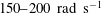 $150{-}200~\text{rad}~\text{s}^{-1}$
for the channels of height
$150{-}200~\text{rad}~\text{s}^{-1}$
for the channels of height
 $0.6$
and 1.8 mm. The magnitude of the frequency can be estimated as the ratio of the speed of shear waves in the wall material,
$0.6$
and 1.8 mm. The magnitude of the frequency can be estimated as the ratio of the speed of shear waves in the wall material,
 $(G/\unicode[STIX]{x1D70C})^{1/2}$
, and the wall thickness. For
$(G/\unicode[STIX]{x1D70C})^{1/2}$
, and the wall thickness. For
 $G\sim 1$
kPa and
$G\sim 1$
kPa and
 $\unicode[STIX]{x1D70C}\sim 10^{3}~\text{kg}~\text{m}^{-3}$
, the shear wave speed is of the order of
$\unicode[STIX]{x1D70C}\sim 10^{3}~\text{kg}~\text{m}^{-3}$
, the shear wave speed is of the order of
 $1~\text{m}~\text{s}^{-1}$
. The wall thickness is approximately 7 mm (figure 1), and so the estimated frequency of oscillations is, to within a proportionality constant, approximately
$1~\text{m}~\text{s}^{-1}$
. The wall thickness is approximately 7 mm (figure 1), and so the estimated frequency of oscillations is, to within a proportionality constant, approximately
 $150~\text{rad}~\text{s}^{-1}$
. This is certainly in quantitative agreement with the experimental observations in the range of
$150~\text{rad}~\text{s}^{-1}$
. This is certainly in quantitative agreement with the experimental observations in the range of
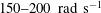 $150{-}200~\text{rad}~\text{s}^{-1}$
. Thus, the measured frequency of oscillations after the wall-flutter transition is well explained on the basis of the shear wave velocity in the solid and the wall thickness. However, it is not clear why the frequency of oscillations is independent of the Reynolds number, and why the frequency depends on whether the flow is laminar or turbulent. It would be necessary to solve the coupled solid–fluid problem in order to determine the values of the resonant frequencies in laminar and turbulent flows.
$150{-}200~\text{rad}~\text{s}^{-1}$
. Thus, the measured frequency of oscillations after the wall-flutter transition is well explained on the basis of the shear wave velocity in the solid and the wall thickness. However, it is not clear why the frequency of oscillations is independent of the Reynolds number, and why the frequency depends on whether the flow is laminar or turbulent. It would be necessary to solve the coupled solid–fluid problem in order to determine the values of the resonant frequencies in laminar and turbulent flows.
6.3 Logarithmic layer in soft-wall turbulence
A striking feature of soft-wall turbulence is the presence of a logarithmic layer close to the wall even at Reynolds numbers as low as 350. The logarithmic layer is observed after the soft-wall transition from both laminar and turbulent flows, but there is no logarithmic layer after the wall-flutter transition. There is no evidence of a viscous sublayer even at distances for 1–2 wall units from the wall; it is not clear if the viscous sublayer is absent or if the thickness is too small to be resolved in the experiments. The spatial extent of the logarithmic layer is approximately
 $2\lesssim (yv_{\ast }/\unicode[STIX]{x1D708})\lesssim 30$
for the channel of height approximately 0.6 mm, and approximately
$2\lesssim (yv_{\ast }/\unicode[STIX]{x1D708})\lesssim 30$
for the channel of height approximately 0.6 mm, and approximately
 $3\lesssim (yv_{\ast }/nu)\lesssim 70$
for the channel of height approximately 1.8 mm. This range is much lower than the range
$3\lesssim (yv_{\ast }/nu)\lesssim 70$
for the channel of height approximately 1.8 mm. This range is much lower than the range
 $30\leqslant (yv_{\ast }/\unicode[STIX]{x1D708})\leqslant 200$
usually quoted for hard-wall turbulence and the spatial extent seems to increase as the Reynolds number increases. The constants in the logarithmic law are different from those for turbulence in a rigid channel at much higher Reynolds number. These constants also seem to depend on the shear modulus of the soft wall and the channel height.
$30\leqslant (yv_{\ast }/\unicode[STIX]{x1D708})\leqslant 200$
usually quoted for hard-wall turbulence and the spatial extent seems to increase as the Reynolds number increases. The constants in the logarithmic law are different from those for turbulence in a rigid channel at much higher Reynolds number. These constants also seem to depend on the shear modulus of the soft wall and the channel height.
As an aside, note that recent very large-scale experiments and simulations (Zagarola & Smits Reference Zagarola and Smits1998; Hoya & Jimenez Reference Hoya and Jimenez2006) suggest that the logarithmic law may be valid only at large distances from the wall,
 $(yv_{\ast }/\unicode[STIX]{x1D708})>200$
or larger, in large-scale experiments and simulations. It is not clear whether the lower limit of
$(yv_{\ast }/\unicode[STIX]{x1D708})>200$
or larger, in large-scale experiments and simulations. It is not clear whether the lower limit of
 $(yv_{\ast }/\unicode[STIX]{x1D708})$
saturates or increases continuously in the high Reynolds number limit, and the von Kármán constant, which was earlier considered to be equal to a universal value of 0.41, is now found to be slightly but distinctly different in channel and pipe flows (Nagib & Chauhan Reference Nagib and Chauhan2008). We do not venture into these discussions, since the logarithmic profile here is certainly different from that in hard-wall-bounded flows.
$(yv_{\ast }/\unicode[STIX]{x1D708})$
saturates or increases continuously in the high Reynolds number limit, and the von Kármán constant, which was earlier considered to be equal to a universal value of 0.41, is now found to be slightly but distinctly different in channel and pipe flows (Nagib & Chauhan Reference Nagib and Chauhan2008). We do not venture into these discussions, since the logarithmic profile here is certainly different from that in hard-wall-bounded flows.
The log law reported here appears to have a different origin than the von Kármán law for the turbulent flow past a rigid surface. In the classical description of wall-bounded turbulence (Tennekes & Lumley Reference Tennekes and Lumley1972; Panton Reference Panton1984), the flow consists of a viscous sublayer close to the wall for
 $(yv_{\ast }/\unicode[STIX]{x1D708})<5$
with a linear profile
$(yv_{\ast }/\unicode[STIX]{x1D708})<5$
with a linear profile
 $(\bar{v}_{x}/v_{\ast })=(yv_{\ast }/\unicode[STIX]{x1D708})$
; a buffer layer for
$(\bar{v}_{x}/v_{\ast })=(yv_{\ast }/\unicode[STIX]{x1D708})$
; a buffer layer for
 $5<(yv_{\ast }/\unicode[STIX]{x1D708})<30$
; and a logarithmic layer for
$5<(yv_{\ast }/\unicode[STIX]{x1D708})<30$
; and a logarithmic layer for
 $30<(yv_{\ast }/\unicode[STIX]{x1D708})<200$
, where the scaled velocity is given by
$30<(yv_{\ast }/\unicode[STIX]{x1D708})<200$
, where the scaled velocity is given by
 $(1/\unicode[STIX]{x1D705})\log (yv_{\ast }/\unicode[STIX]{x1D708})+A$
, where
$(1/\unicode[STIX]{x1D705})\log (yv_{\ast }/\unicode[STIX]{x1D708})+A$
, where
 $\unicode[STIX]{x1D705}$
is the von Kármán constant (Townsend Reference Townsend1956; Rotta Reference Rotta1962). The original model of von Kármán and Prandtl (George Reference George2007) for the logarithmic layer is based on a constant stress in the near-wall region coupled with an eddy viscosity which increases proportional to the distance from the wall. This is clearly not applicable in the present case – a comparison of figures 3(e,f) and 12(e,f) shows that the stress is certainly not a constant in the region where the velocity follows the log law, and the viscous stress is larger than the Reynolds stress in this region, so the eddy viscosity model cannot be reliably used. Asymptotic matching techniques have also been used to derive the logarithmic velocity profile. Here, the strain rate in the near-wall region, where the length is scaled by
$\unicode[STIX]{x1D705}$
is the von Kármán constant (Townsend Reference Townsend1956; Rotta Reference Rotta1962). The original model of von Kármán and Prandtl (George Reference George2007) for the logarithmic layer is based on a constant stress in the near-wall region coupled with an eddy viscosity which increases proportional to the distance from the wall. This is clearly not applicable in the present case – a comparison of figures 3(e,f) and 12(e,f) shows that the stress is certainly not a constant in the region where the velocity follows the log law, and the viscous stress is larger than the Reynolds stress in this region, so the eddy viscosity model cannot be reliably used. Asymptotic matching techniques have also been used to derive the logarithmic velocity profile. Here, the strain rate in the near-wall region, where the length is scaled by
 $(\unicode[STIX]{x1D708}/v_{\ast })$
, and the strain rate in the outer flow, where the length is scaled by the channel height, are matched using an ‘intermediate limit process’ (Tennekes & Lumley Reference Tennekes and Lumley1972). In the present system, the Reynolds number is relatively low, and the logarithmic layer seems to extend up to approximately 20 %–30 % of the channel height on both sides, as shown in figures 3(f) and 12(f). It is difficult to justify an asymptotic matching procedure.
$(\unicode[STIX]{x1D708}/v_{\ast })$
, and the strain rate in the outer flow, where the length is scaled by the channel height, are matched using an ‘intermediate limit process’ (Tennekes & Lumley Reference Tennekes and Lumley1972). In the present system, the Reynolds number is relatively low, and the logarithmic layer seems to extend up to approximately 20 %–30 % of the channel height on both sides, as shown in figures 3(f) and 12(f). It is difficult to justify an asymptotic matching procedure.
6.4 Practical implications
The present experiments show that the hydroelastic instability, hitherto observed only in external flows, is of relevance in internal flows as well, but the instability is sensitive to the constraints on the soft wall. The instability is observed at the unrestrained wall at a Reynolds number of about 1000, but it is observed at the fixed bottom wall at a Reynolds number of 3500. Physiological flows in constrained channels are not likely to be affected by the wall-flutter instability, but this transition provides an opportunity for controlling the instability by designing suitable walls.
The soft-wall transitions observed here necessitates a re-examination of our current understanding of transition and turbulence in the flow through soft conduits, such as physiological flows. It has hitherto been assumed that this transition is important only if the transition Reynolds number is lower than that for hard-wall transition. This requires very soft walls or very small dimensions, to attain a sufficiently small value of the parameter
 $\unicode[STIX]{x1D6F4}$
. Here, we find that the soft-wall transition takes place from laminar and turbulent flow, and is of relevance of all values of
$\unicode[STIX]{x1D6F4}$
. Here, we find that the soft-wall transition takes place from laminar and turbulent flow, and is of relevance of all values of
 $\unicode[STIX]{x1D6F4}$
. The experiments also show that soft-wall turbulence constitutes a specific type of turbulence, distinct from hard-wall turbulence, due to the participation of the soft wall in turbulence generation. In this case, the flow, friction and transport characteristics, especially in the near-wall region, are likely to be very different from those for hard-wall turbulence. A good understanding of soft-wall turbulence as a distinct class of turbulence, and the coupling between fluid and wall dynamics in this class of turbulence, is necessary for accurate modelling of physiological flows.
$\unicode[STIX]{x1D6F4}$
. The experiments also show that soft-wall turbulence constitutes a specific type of turbulence, distinct from hard-wall turbulence, due to the participation of the soft wall in turbulence generation. In this case, the flow, friction and transport characteristics, especially in the near-wall region, are likely to be very different from those for hard-wall turbulence. A good understanding of soft-wall turbulence as a distinct class of turbulence, and the coupling between fluid and wall dynamics in this class of turbulence, is necessary for accurate modelling of physiological flows.
Acknowledgements
The authors would like to thank the Department of Science and Technology, Government of India for financial support; facilities made available and advice provided by Professors O. N. Ramesh, J. Dey, R. Govardhan, J. H. Arakeri, A. Ghosh, S. Basu, S. Bose and S. V. Kailas. The authors are grateful to Professors A. C. Mandal, Dr M. K. S. Verma, Mr J. Suryanarayana Murthy, Mr Phani Kumar, Mr Narsing Jha, Mr V. Swamybabu, Mr S. Jaju, Mr A. Tyagi and Mr U. Abbasi for instructive discussions. A brief summary of this work is accepted for presentation at the Tenth International Symposium on Turbulence and Shear Flow Phenomena, 2017.
Table 3. The weight in grams of Acrylamide (AA), Methylene Bisacrylamide (MBA), Ammonium Persulphate (APS), Tetramethylenediamine (TEMED); the weight fraction of water in the gel
 $W_{H_{2}O}$
, and the average values of the storage and loss moduli,
$W_{H_{2}O}$
, and the average values of the storage and loss moduli,
 $G^{\prime }$
and
$G^{\prime }$
and
 $G^{\prime \prime }$
, in the frequency range 10–100 Hz, and the steady compression modulus
$G^{\prime \prime }$
, in the frequency range 10–100 Hz, and the steady compression modulus
 $K$
, as a function of the composition of the gel.
$K$
, as a function of the composition of the gel.

Appendix A. Channel fabrication and characterisation of the polyacrylamide gel
Channels were made of polyacrylamide gels with three different compositions, shown in table 3. The final water mass fraction in these gels were 0.75, 0.92 and 0.94. The gel with water mass fraction 0.75, which has a shear modulus of approximately 15.89 kPa, is used for making the development section, since it is sufficiently hard that the soft-wall and wall-flutter transitions are not observed for the range of Reynolds numbers examined in the experiments. This is also used for validation of the hard-wall turbulence in a rigid channel in appendix B. The gel with mass fractions 0.92 and 0.94 have shear moduli 2.19 and 0.75 kPa respectively, and these are used for the experiments on soft-wall and wall-flutter transitions.
The channel fabrication procedure is as follows. First, a hollow rectangular mould of length approximately 20 cm, width 2.5 cm and height 1.5 cm is constructed using glass plates, as shown in figure 17(a). A glass slide of width 1 cm and one of two heights, 0.5 mm and 1.5 mm, is held at the centre of the channel using a Teflon spacer. One end of the mould is sealed, the mould is held vertically and the gelation mixture with concentrations appropriate for the development section is poured in up to a height of 10 cm, as shown in figure 17(b). The gelation mixture is stored for ten minutes at room temperature for completion of the reaction. After this, polymer mixture with concentration appropriate for the test section is poured into the mould for the remaining height of 10 cm, as shown in figure 17(c), and the mould is kept at room temperature for another ten minutes to complete gelation of the test section.

Figure 17. Fabrication procedure: (a) glass mould with side and bottom glass plates and with top glass plate covering one half of the channel length and glass template held in place by sticking tape, (b) channel held with axis vertical and prepolymer for the development section is poured into one half of the channel, development section is cured, (c) channel is held horizontal and prepolymer for test section is poured into the other half of the channel, test section cured, (d) polymer swollen in water and the glass slide and glass top and side walls removed to obtain a rectangular bore in a block of polyacrylamide gel on a glass substrate.
The mould is then placed in a water bath with its axis horizontal and the top and side glass plates are carefully removed. For experiments with a fixed top wall, only the side plates are removed and the top and bottom plates are retained. The gel is then allowed to swell in a water bath for approximately three weeks and then the glass slide at the centre of the gel is carefully removed, resulting in a rectangular channel in the centre of the gel, as shown in figure 17(d). After swelling, the lengths of the development and test sections increase to approximately 13 cm and 14 cm respectively, and the width of the channel increases to approximately 1.3 cm, as shown in figure 1(a). When the glass slide template used at the centre of the channel is of height 0.5/1.5 mm, the final channel height after swelling increases to approximately 0.6 mm/1.8 mm, as shown in figure 1(b). One issue that has been of concern is regarding the effect of gradients in the gel elastic properties on the stability characteristics; it has been reported that these could have a significant effect at low Reynolds numbers (Gkanis & Kumar Reference Gkanis and Kumar2006). In the present polyacrylamide gels, these gradients are not likely to be significant, since these are prepared using the same protocol as those in gel chromatography, and are known to be very homogeneous.
The frequency-dependent storage and loss modulus of the gel was determined using a AR 1000 N Rheometer from TA Instruments. A slab of gel of height 2 mm was fabricated using the same reactant compositions and curing procedure as those used for the soft channels. These were placed on the bottom plate of the rheometer, the top plate was lowered and the oscillatory rheology measurements were carried out in stress controlled mode over a frequency range 0.1–100 Hz using a maximum stress oscillation of 50 Pa. The measurements were repeated three times for three different samples with identical compositions and preparation protocols, and the mean and the standard deviation were calculated over these three different measurements. The results of the oscillatory measurements are shown in figure 18, and the error bars show one standard deviation above and below the mean value. It is evident that the storage modulus is nearly independent of frequency over the range of frequencies studied, although there is some variation in the limit of low frequency. The loss modulus is approximately an order of magnitude smaller than the storage modulus, and it shows greater variation with frequency. The average of the storage modulus in the range
 $10{-}100~\text{Hz}$
is denoted the plateau modulus, provided in table 3, is used for calculating relevant dimensionless groups. The steady compression modulus is also determined using the AR 1000N rheometer using the following procedure. The gel slab is placed on the bottom plate of the rheometer and the top plate is lowered until a normal stress is detected. The plate is further lowered in increments of approximately
$10{-}100~\text{Hz}$
is denoted the plateau modulus, provided in table 3, is used for calculating relevant dimensionless groups. The steady compression modulus is also determined using the AR 1000N rheometer using the following procedure. The gel slab is placed on the bottom plate of the rheometer and the top plate is lowered until a normal stress is detected. The plate is further lowered in increments of approximately
 $5~\unicode[STIX]{x03BC}\text{m}$
, and the normal stress on the top plate is recorded. The normal stress
$5~\unicode[STIX]{x03BC}\text{m}$
, and the normal stress on the top plate is recorded. The normal stress
 $\unicode[STIX]{x1D70E}$
is plotted as a function of the normal compressive strain
$\unicode[STIX]{x1D70E}$
is plotted as a function of the normal compressive strain
 $\unicode[STIX]{x1D716}$
, which is the ratio of the displacement and the initial thickness. The results of the measurements for three different values of the gel composition are shown in figure 19. The compression modulus is the slope of the stress–strain curve in the limit of zero strain, as shown in figure 19. The compression modulus is also tabulated as a function of the gel composition in table 3.
$\unicode[STIX]{x1D716}$
, which is the ratio of the displacement and the initial thickness. The results of the measurements for three different values of the gel composition are shown in figure 19. The compression modulus is the slope of the stress–strain curve in the limit of zero strain, as shown in figure 19. The compression modulus is also tabulated as a function of the gel composition in table 3.

Figure 18. The frequency-dependent storage modulus (a) and loss modulus (b) for gels with water weight fraction 0.75 (○), 0.92 (▵) and 0.94 (▿).

Figure 19. The normal stress
 $\unicode[STIX]{x1D70E}_{n}$
as a function of the compressive strain
$\unicode[STIX]{x1D70E}_{n}$
as a function of the compressive strain
 $\unicode[STIX]{x1D700}$
for gels with water weight fraction 0.75 (○), 0.92 (▵) and 0.94 (▿). The compression modulus is equal to the slope of the dashed lines in the figure.
$\unicode[STIX]{x1D700}$
for gels with water weight fraction 0.75 (○), 0.92 (▵) and 0.94 (▿). The compression modulus is equal to the slope of the dashed lines in the figure.
The roughness of the walls of the channel were measured by first slicing the channel and then using a WYKO NT 1100 optical profilometer. Four representative surface patches of area
 $1~\text{mm}\times 1~\text{mm}$
were chosen, and the height profile in these patches were measured. The root mean square of the deviation of the height from the average value was found to be approximately
$1~\text{mm}\times 1~\text{mm}$
were chosen, and the height profile in these patches were measured. The root mean square of the deviation of the height from the average value was found to be approximately
 $1.06~\unicode[STIX]{x03BC}\text{m}$
, thereby resulting in an average roughness of approximately 1 %. For comparison, the height variation in custom fabricated pipes for low noise pipe flow experiments is of the order of
$1.06~\unicode[STIX]{x03BC}\text{m}$
, thereby resulting in an average roughness of approximately 1 %. For comparison, the height variation in custom fabricated pipes for low noise pipe flow experiments is of the order of
 $10~\unicode[STIX]{x03BC}\text{m}$
(Darbyshire & Mullin Reference Darbyshire and Mullin1995; Hof, Juel & Mullin Reference Hof, Juel and Mullin2003), although the roughness is smaller at approximately 0.05 % for a pipe of diameter 2 cm.
$10~\unicode[STIX]{x03BC}\text{m}$
(Darbyshire & Mullin Reference Darbyshire and Mullin1995; Hof, Juel & Mullin Reference Hof, Juel and Mullin2003), although the roughness is smaller at approximately 0.05 % for a pipe of diameter 2 cm.
Appendix B. Validation
In order to validate the PIV measurements for a laminar flow, velocity profiles were determined at a location 0.5 cm upstream of the joint between the development and test sections, where the velocity profile is expected to be fully developed. The results, shown in figure 20, confirm that mean velocity profile is parabolic at all Reynolds numbers up to approximately 800 in the channel with height approximately 0.6 mm. The measured values of the root mean square of the fluctuating velocities are also shown, scaled by the average velocity. These measurements provide the limit of the experimental resolution in the velocity measurements for the following reason. The time delay in the PIV pulses is adjusted so as to capture the maximum flow velocity. When this is done, there is a limitation in the resolution of the minimum velocity which can be measured, which scales approximately linearly with the flow velocity, as shown in figure 20. This does not affect the mean velocity, since the positive and negative fluctuations in the PIV measurements average to zero. However, since we are adding up both positive and negative fluctuations when calculating the root mean square velocities, this error is visible even close to the wall in the PIV measurements. The background level of fluctuations in the streamwise root mean square velocity,
 $v_{x}^{\prime }$
, is approximately 4 % of the average velocity, while that of the cross-stream root mean square velocity
$v_{x}^{\prime }$
, is approximately 4 % of the average velocity, while that of the cross-stream root mean square velocity
 $v_{y}^{\prime }$
is approximately 2 % of the average velocity. The correlation
$v_{y}^{\prime }$
is approximately 2 % of the average velocity. The correlation
 $\langle v_{x}^{\prime }v_{y}^{\prime }\rangle$
is approximately
$\langle v_{x}^{\prime }v_{y}^{\prime }\rangle$
is approximately
 $10^{-3}$
when scaled by the square of the average velocity. This provides an estimate of the background level of fluctuations in the PIV measurements of the mean and root mean square velocities. The experimental results are relevant only if they exceed this resolution limit in the PIV measurements.
$10^{-3}$
when scaled by the square of the average velocity. This provides an estimate of the background level of fluctuations in the PIV measurements of the mean and root mean square velocities. The experimental results are relevant only if they exceed this resolution limit in the PIV measurements.

Figure 20. The cross-stream variation of
 $(\bar{v}_{x}/\bar{v})$
(a),
$(\bar{v}_{x}/\bar{v})$
(a),
 $(v_{x}^{\prime }/\bar{v})$
(b),
$(v_{x}^{\prime }/\bar{v})$
(b),
 $(v_{y}^{\prime }/\bar{v})$
(c) and
$(v_{y}^{\prime }/\bar{v})$
(c) and
 $(\langle v_{x}^{\prime }v_{y}^{\prime }\rangle /\bar{v}^{2})$
(d), at the streamwise location 0.5 cm upstream of the junction between the development and test sections at Reynolds number 217 (○), 403 (▵), 482 (▿), 597 (◃), 662 (▹) and 814 (♢) for a channel with height approximately 0.6 mm in the undeformed state, when the walls are made with shear modulus 0.75 kPa. The dashed curve in panel (a) shows a parabolic velocity profile with the same mean velocity.
$(\langle v_{x}^{\prime }v_{y}^{\prime }\rangle /\bar{v}^{2})$
(d), at the streamwise location 0.5 cm upstream of the junction between the development and test sections at Reynolds number 217 (○), 403 (▵), 482 (▿), 597 (◃), 662 (▹) and 814 (♢) for a channel with height approximately 0.6 mm in the undeformed state, when the walls are made with shear modulus 0.75 kPa. The dashed curve in panel (a) shows a parabolic velocity profile with the same mean velocity.
In order to validate the turbulence measurements, experiments were carried out in a channel with test section made with gel of shear modulus 15.89 kPa, fabricated using the procedure shown in figure 17. Even though the development and test sections are made with the same concentration, we use the same two-step process shown in figure 17 to ensure that the joint between the development and test sections does not create any artefact in the flow. The optical set-up and the PIV measurement techniques are identical to those used for the experiments with soft gels. The measurements were carried out at a Reynolds number of 3500 based on the flow rate and the channel width. Simulations have also been carried out using the direct numerical simulation (DNS) procedure outlined in Goswami & Kumaran (Reference Goswami and Kumaran2011) at the same Reynolds number. The results of the experiments and simulation, compared in figure 21, show that the profiles of the mean and root mean square fluctuating velocities are accurately measured in the experiments, thus validating the experimental procedure. The logarithmic velocity profile is captured in the von Kármán plot of the velocity profile in figure 21(d), and the two points nearest the wall fit the linear profile in the viscous sublayer.

Figure 21. The cross-stream variation of
 $\bar{v}_{x}$
(a),
$\bar{v}_{x}$
(a),
 $v_{x}^{\prime }$
▵ and
$v_{x}^{\prime }$
▵ and
 $v_{y}^{\prime }$
▿ (b) and
$v_{y}^{\prime }$
▿ (b) and
 $\langle v_{x}^{\prime }v_{y}^{\prime }\rangle$
(c); and the variation of
$\langle v_{x}^{\prime }v_{y}^{\prime }\rangle$
(c); and the variation of
 $(v_{x}/v_{\ast })$
with
$(v_{x}/v_{\ast })$
with
 $(yv_{\ast }/\unicode[STIX]{x1D708})$
(d), for a channel with height approximately 1.8 mm in the undeformed state when the wall is made of shear modulus 15.89 kPa at a Reynolds number of 3500 based on the average velocity and channel height. The symbols are the experimental results, and the lines are the results from DNS simulations expressed in wall units. In panel (d), the dotted curve is
$(yv_{\ast }/\unicode[STIX]{x1D708})$
(d), for a channel with height approximately 1.8 mm in the undeformed state when the wall is made of shear modulus 15.89 kPa at a Reynolds number of 3500 based on the average velocity and channel height. The symbols are the experimental results, and the lines are the results from DNS simulations expressed in wall units. In panel (d), the dotted curve is
 $(v_{x}/v_{\ast })=(yv_{\ast }/\unicode[STIX]{x1D708})$
, and the dashed line is
$(v_{x}/v_{\ast })=(yv_{\ast }/\unicode[STIX]{x1D708})$
, and the dashed line is
 $2.44\log (yv_{\ast }/\unicode[STIX]{x1D708})+5.5$
.
$2.44\log (yv_{\ast }/\unicode[STIX]{x1D708})+5.5$
.

Figure 22. The variation of height along the channel length when the walls in the test section are made with shear modulus 0.75 kPa (solid line) and 2.19 kPa (dashed line). Panel (a) shows the height variation for a channel with height approximately 0.6 mm at Reynolds number 270 (○), 298 (▵), 366 (▿), 557 (◃), 785 (▹) and 923 (♢) for a channel with walls made of shear modulus 0.75 kPa and at Reynolds number 214 (○), 398 (▵), 477 (▿), 768 (◃), 1050 (▹) when the walls are made of shear modulus 2.19 kPa. Panel (b) shows the height variation for a channel with height approximately 1.8 mm at Reynolds number 1360 (○), 1660 (▵), 1900 (▿), 2340 (◃), 2660 (▹), 2850 (♢) and 3200
 $(\times )$
.
$(\times )$
.

Figure 23. The variation of
 $(\unicode[STIX]{x0394}h/h_{0})$
as a function of Reynolds number when the walls are made of gel with shear modulus 0.75 kPa (○, solid line) and 2.19 kPa (▵, dashed line) when the height of the undeformed channel is approximately 0.6 mm (a) and 1.8 mm (b). The Reynolds number for the soft-wall and wall-flutter transitions are shown using the labels SW and WF respectively.
$(\unicode[STIX]{x0394}h/h_{0})$
as a function of Reynolds number when the walls are made of gel with shear modulus 0.75 kPa (○, solid line) and 2.19 kPa (▵, dashed line) when the height of the undeformed channel is approximately 0.6 mm (a) and 1.8 mm (b). The Reynolds number for the soft-wall and wall-flutter transitions are shown using the labels SW and WF respectively.
Table 4. The deformation
 $(\unicode[STIX]{x0394}h/h_{0})_{max}$
and the maximum wall slope
$(\unicode[STIX]{x0394}h/h_{0})_{max}$
and the maximum wall slope
 $(\text{d}h/\text{d}x)_{max}$
at the Reynolds numbers corresponding to the soft-wall (SW) and wall-flutter (WF) transitions for channels of undeformed height
$(\text{d}h/\text{d}x)_{max}$
at the Reynolds numbers corresponding to the soft-wall (SW) and wall-flutter (WF) transitions for channels of undeformed height
 $h_{0}$
made of walls with shear modulus
$h_{0}$
made of walls with shear modulus
 $G$
.
$G$
.

Appendix C. Channel deformation
The channel deformation in the soft section due to the applied pressure gradient is first characterised by measuring the channel height along the midplane in the spanwise direction (vertical line in figure 1 c), where the deformation is a maximum. The variation in height with downstream distance is shown in figure 22 for channels with two different shear moduli in the soft section. In the absence of flow, the channels have a uniform height of approximately 0.6 mm and 1.8 mm independent of downstream distance.
In the experimental results, we note that there are two specific Reynolds numbers of interest – the first where there is a soft-wall transition and the second where flutter is observed at the wall of the channel. The maximum deformation and the maximum slope at these Reynolds numbers is listed in table 4. Although there is a substantial deformation of the channel at high Reynolds numbers, the slope of the wall at the transition Reynolds numbers for the soft-wall and wall-flutter transition are numerically small in the experiments. The deformation is a maximum at a distance of about 5 cm downstream of the entrance of the test section. Many of the results presented are at locations beyond 8 cm of the entrance to the test section, where there is relatively little expansion, because the difference between the local pressure and the outlet pressure is much smaller than the pressure difference across the channel. Due to this small slope, computational fluid dynamics (CFD) simulations carried out using ANSYS FLUENT CFD package, discussed in §§ 2.4 and 3.1 of Verma & Kumaran (Reference Verma and Kumaran2013) and § 2.2 Srinivas & Kumaran (Reference Srinivas and Kumaran2015), indicate that the velocity profile along the central plane in the spanwise direction is not discernibly different from a parabolic flow.
Due to the variation in the height of the channel, there is also a local variation in the Reynolds number calculated for the velocity profile along the central plane in the spanwise direction (vertical line in figure 1 c). Here, the profile-averaged streamwise mean velocity is defined as,
 $$\begin{eqnarray}\displaystyle \bar{v}_{x}^{(p)}(x)=\frac{1}{h}\int _{0}^{h}\,\text{d}y\,\bar{v}_{x}(y), & & \displaystyle\end{eqnarray}$$
where
 $\bar{v}_{x}(y)$
is the mean velocity profile measured along the central plane in the spanwise direction at streamwise location
$\bar{v}_{x}(y)$
is the mean velocity profile measured along the central plane in the spanwise direction at streamwise location
 $x$
, and
$x$
, and
 $h$
is the local height. The Reynolds number for the velocity profile along the central plane is defined as
$h$
is the local height. The Reynolds number for the velocity profile along the central plane is defined as
 $$\begin{eqnarray}\displaystyle Re^{(p)}=\frac{\unicode[STIX]{x1D70C}\bar{v}_{x}^{(p)}h}{\unicode[STIX]{x1D702}}. & & \displaystyle\end{eqnarray}$$
This Reynolds number is, in general, higher than the Reynolds number
 $Re$
based on the flow rate (2.1), because the flow retardation at the side walls in the spanwise direction results in a higher velocity along the centreline, and due to the increase in height caused by the applied pressure gradient. The profile Reynolds number
$Re$
based on the flow rate (2.1), because the flow retardation at the side walls in the spanwise direction results in a higher velocity along the centreline, and due to the increase in height caused by the applied pressure gradient. The profile Reynolds number
 $Re^{(p)}$
is shown as a function of the Reynolds number based on the flow rate
$Re^{(p)}$
is shown as a function of the Reynolds number based on the flow rate
 $Re$
(2.1) in figure 24.
$Re$
(2.1) in figure 24.
For the channel with undeformed height approximately 0.6 mm made with gel of shear modulus 0.75 kPa,
 $Re^{(p)}$
is significantly higher than
$Re^{(p)}$
is significantly higher than
 $Re$
at the location II (figure 1), due to the large increase in the height along the central plane at high Reynolds numbers, as shown in figure 22(a). At the downstream locations III and IV,
$Re$
at the location II (figure 1), due to the large increase in the height along the central plane at high Reynolds numbers, as shown in figure 22(a). At the downstream locations III and IV,
 $Re^{(p)}$
exceeds
$Re^{(p)}$
exceeds
 $Re$
by less than 5 % at the transition Reynolds number of about 300, and less than 10 % at the Reynolds number of approximately 500 where flutter is first observed. Similar ratios of
$Re$
by less than 5 % at the transition Reynolds number of about 300, and less than 10 % at the Reynolds number of approximately 500 where flutter is first observed. Similar ratios of
 $Re^{(p)}/Re$
are obtained at the soft-wall transition at a Reynolds number of 480 and the inception of flutter at a Reynolds number of approximately 760 for a channel of undeformed height 0.6 mm with walls made of shear modulus 2.19 kPa. For the channel with height approximately 1.8 mm in the absence of deformation, the
$Re^{(p)}/Re$
are obtained at the soft-wall transition at a Reynolds number of 480 and the inception of flutter at a Reynolds number of approximately 760 for a channel of undeformed height 0.6 mm with walls made of shear modulus 2.19 kPa. For the channel with height approximately 1.8 mm in the absence of deformation, the
 $Re^{(p)}$
exceeds
$Re^{(p)}$
exceeds
 $Re$
by approximately 5 % or smaller for the entire range of Reynolds numbers considered here, as shown in figure 24(b).
$Re$
by approximately 5 % or smaller for the entire range of Reynolds numbers considered here, as shown in figure 24(b).

Figure 24. The Reynolds number
 $Re^{(p)}$
based on the profile-averaged velocity as a function of the Reynolds number
$Re^{(p)}$
based on the profile-averaged velocity as a function of the Reynolds number
 $Re$
based on the flow rate when the wall is made of shear modulus 0.75 kPa (solid line) and shear modulus 2.19 kPa (dashed line) when the height of the channel is approximately 0.6 mm (a) and approximately 1.8 mm (b) at different downstream locations I (○), II (▵), III (▿) and IV (♢), shown in figure 1(a).
$Re$
based on the flow rate when the wall is made of shear modulus 0.75 kPa (solid line) and shear modulus 2.19 kPa (dashed line) when the height of the channel is approximately 0.6 mm (a) and approximately 1.8 mm (b) at different downstream locations I (○), II (▵), III (▿) and IV (♢), shown in figure 1(a).


