1 Introduction
In recent years, the specialities of micro- and nanoscale science have been routinely exploited in diverse microfluidic applications such as cell cultures (Rhee et al.
Reference Rhee, Taylor, Tu, Cribbs, Cotman and Jeon2005), clinical diagnostics (Christodoulides et al.
Reference Christodoulides, Tran, Floriano, Rodriguez, Goodey, Ali, Neikirk and McDevitt2002), immunoassays (Wang et al.
Reference Wang, Ibáñez, Chatrathi and Escarpa2001), DNA analysis (Doyle et al.
Reference Doyle, Bibette, Bancaud and Viovy2002) and environmental monitoring (Bromberg & Mathies Reference Bromberg and Mathies2003). The microscale applications are found to have some distinct advantages over their macroscopic counterparts such as, (i) usage and control of lesser amounts of materials (Haeberle & Zengerle Reference Haeberle and Zengerle2007); (ii) availability of higher surface to volume ratio; (iii) high performance due to process intensification (Mark et al.
Reference Mark, Haeberle, Roth, von Stetten and Zengerle2010); and (iv) superior control over the process parameters (Vilkner, Janasek & Manz Reference Vilkner, Janasek and Manz2004). It is now well understood that for efficient and time bound operations, the existing microscale chemical and biological applications require rapid mixing of fluid streams inside the microfluidic devices (Hertzog et al.
Reference Hertzog, Ivorra, Mohammadi, Bakajin and Santiago2006; Janasek, Franzke & Manz Reference Janasek, Franzke and Manz2006; Samiei, Tabrizian & Hoorfar Reference Samiei, Tabrizian and Hoorfar2016). However, the conventional pressure-driven microfluidic flows are often limited by low values of the Reynolds number (
 $Re$
), which results in large diffusive time and length scales of mixing owing to the dominance of the viscous force over the inertial one (Stroock et al.
Reference Stroock, Dertinger, Ajdari, Mezić, Stone and Whitesides2002; El Moctar, Aubry & Batton Reference El Moctar, Aubry and Batton2003). In the macroscopic processes, the diffusion limited mixing lengths are improved by the generation of auxiliary transport pathways such as turbulence. In contrast, for the microscale processes, the large frictional resistance originating from the confining boundaries pose multifarious challenges towards this end. Thus, of late, the enhancement of momentum, heat and mass transport in microscale processes has become one of the major areas of fluid dynamical research (Stone, Stroock & Ajdari Reference Stone, Stroock and Ajdari2004).
$Re$
), which results in large diffusive time and length scales of mixing owing to the dominance of the viscous force over the inertial one (Stroock et al.
Reference Stroock, Dertinger, Ajdari, Mezić, Stone and Whitesides2002; El Moctar, Aubry & Batton Reference El Moctar, Aubry and Batton2003). In the macroscopic processes, the diffusion limited mixing lengths are improved by the generation of auxiliary transport pathways such as turbulence. In contrast, for the microscale processes, the large frictional resistance originating from the confining boundaries pose multifarious challenges towards this end. Thus, of late, the enhancement of momentum, heat and mass transport in microscale processes has become one of the major areas of fluid dynamical research (Stone, Stroock & Ajdari Reference Stone, Stroock and Ajdari2004).
Over the years, various pathways have been explored to engender auxiliary transport mechanisms in microfluidic flows with the help of active and passive triggers. For example, the innovations associated with groovy or twisted channels (Bertsch et al. Reference Bertsch, Heimgartner, Cousseau and Renaud2001; Stroock et al. Reference Stroock, Dertinger, Ajdari, Mezić, Stone and Whitesides2002; Verma et al. Reference Verma, Ganneboyina, Vinayak and Ghatak2008), multi-lamination of flow paths (Hinsmann et al. Reference Hinsmann, Frank, Svasek, Harasek and Lendl2001), serpentine channels (Simonnet & Groisman Reference Simonnet and Groisman2005) and viscous fingering of fluids (Jha, Cueto-Felgueroso & Juanes Reference Jha, Cueto-Felgueroso and Juanes2011) disclose passive modes of enhanced momentum transport. In comparison, the active triggers require the support of the external fields such as applications of thermal (Wall & Wilson Reference Wall and Wilson1996), or acoustic waves (Rife et al. Reference Rife, Bell, Horwitz, Kabler, Auyeung and Kim2000), magnetic (Yi, Qian & Bau Reference Yi, Qian and Bau2002), or electrokinetic forces (Oddy, Santiago & Mikkelsen Reference Oddy, Santiago and Mikkelsen2001; Chen et al. Reference Chen, Lin, Lele and Santiago2005; Posner & Santiago Reference Posner and Santiago2006; Zhao & Bau Reference Zhao and Bau2007; Harnett et al. Reference Harnett, Templeton, Dunphy-Guzman, Senousy and Kanouff2008; Posner, Pérez & Santiago Reference Posner, Pérez and Santiago2012; Wang, Yang & Zhao Reference Wang, Yang and Zhao2014; Ding & Wong Reference Ding and Wong2015; Wang et al. Reference Wang, Yang, Zhao and Chen2016). However, the enhancement of momentum, heat and mass diffusivities with the help of in situ disturbances inside microfluidic devices remains one of the long standing challenges in this regard. For example, the electrohydrodynamic (EHD) instabilities due to the electrokinetic phenomena instigated by conductivity gradients between the fluids have been explored only recently (Posner et al. Reference Posner, Pérez and Santiago2012; Wang et al. Reference Wang, Yang and Zhao2014; Ding & Wong Reference Ding and Wong2015; Wang et al. Reference Wang, Yang, Zhao and Chen2016).
In the present study, we investigate the consequence of an EHD phenomenon to develop laminar, transitional and chaotic flow regimes. The phenomenon originates due to injection of ions into a pair of miscible fluids undergoing a pressure-driven stratified flow in a microchannel. The miscible fluids are considered to have higher viscosity contrast and lower electrical conductivities to explore the cumulative effects of electric field stress and viscosity stratification. The major interests here are twofold: (i) to experimentally investigate the various regimes of instabilities in the aforementioned system leading to chaotic mixing of the fluid streams, and (ii) to theoretically analyse the linear regime of instability to predict their nature and onset conditions. The study is pertinent due to its significance in a plurality of futuristic applications such as microfluidic mixing in drug delivery systems, heat transfer enhancement, reactions in micro reactors, among others.
The prior art related to the stability of viscosity stratified miscible flows suggests that Craik (Reference Craik1969) was among the pioneers who identified that these flows can be more stable than the immiscible ones owing to the damping of the perturbations near the interface due to molecular diffusion. Much later, Ranganathan & Govindarajan (Reference Ranganathan and Govindarajan2001) theoretically identified the influence of the location of the viscosity stratified layer with respect to the critical layer of the perturbation. Subsequently, Ern, Charru & Luchini (Reference Ern, Charru and Luchini2003) showed that the effect of molecular diffusion is not always stabilizing. They identified that for moderate values of Péclet number (
 $400\leqslant Pe\leqslant 10\,000$
), the perturbation at a thicker interface might grow to destabilize the system. Later, Govindarajan (Reference Govindarajan2004) identified an overlap mode of instability, distinct from the classical Tollmien–Schlichting (TS) and inviscid modes, obtained when the critical layer of the most dominant disturbance merges with the viscosity stratified layer. More recently, Selvam et al. (Reference Selvam, Merk, Govindarajan and Meiburg2007, Reference Selvam, Talon, Lesshafft and Meiburg2009) noted that miscible core–annular flows can be unstable beyond a critical viscosity ratio, when the lighter phase occupies the annular region. The observations in this study uncovered some of the exceptions to the claims of Ranganathan & Govindarajan (Reference Ranganathan and Govindarajan2001). Talon & Meiburg (Reference Talon and Meiburg2011) performed the stability analysis of miscible fluids with strong viscosity stratification in the Stokes flow regime (
$400\leqslant Pe\leqslant 10\,000$
), the perturbation at a thicker interface might grow to destabilize the system. Later, Govindarajan (Reference Govindarajan2004) identified an overlap mode of instability, distinct from the classical Tollmien–Schlichting (TS) and inviscid modes, obtained when the critical layer of the most dominant disturbance merges with the viscosity stratified layer. More recently, Selvam et al. (Reference Selvam, Merk, Govindarajan and Meiburg2007, Reference Selvam, Talon, Lesshafft and Meiburg2009) noted that miscible core–annular flows can be unstable beyond a critical viscosity ratio, when the lighter phase occupies the annular region. The observations in this study uncovered some of the exceptions to the claims of Ranganathan & Govindarajan (Reference Ranganathan and Govindarajan2001). Talon & Meiburg (Reference Talon and Meiburg2011) performed the stability analysis of miscible fluids with strong viscosity stratification in the Stokes flow regime (
 $Re\rightarrow 0$
), and observed four distinct modes of instability in which two were interfacial while the other two were bulk modes. They proposed that these instabilities grew due to the phase shift between vorticity and interfacial perturbations. Subsequently, a number of works showed the influence of miscibility (Sahu & Govindarajan Reference Sahu and Govindarajan2016), inclination (Scoffoni, Lajeunesse & Homsy Reference Scoffoni, Lajeunesse and Homsy2001; d’Olce et al.
Reference d’Olce, Martin, Rakotomalala, Salin and Talon2009; Ghosh & Usha Reference Ghosh and Usha2016) and variable density (Talon, Goyal & Meiburg Reference Talon, Goyal and Meiburg2013) on the different modes of instability. Apart from macroscopic flows, microscale flows of miscible fluids have also been explored theoretically (Tan & Homsy Reference Tan and Homsy1986; Preziosi, Chen & Joseph Reference Preziosi, Chen and Joseph1989; Chen & Meiburg Reference Chen and Meiburg1996), as well as experimentally (Petitjeans & Maxworthy Reference Petitjeans and Maxworthy1996; Lajeunesse et al.
Reference Lajeunesse, Martin, Rakotomalala, Salin and Yortsos1999). Interestingly, these studies indicate that the dominance (weakness) of the frictional (inertial) force at the microscale often disallows intermixing of the fluid layers to provide a kinetic stability at the stratified interface, even when the molecular diffusivities of the fluid layers are high, leading to a weaker capacity of heat, mass and momentum transfer.
$Re\rightarrow 0$
), and observed four distinct modes of instability in which two were interfacial while the other two were bulk modes. They proposed that these instabilities grew due to the phase shift between vorticity and interfacial perturbations. Subsequently, a number of works showed the influence of miscibility (Sahu & Govindarajan Reference Sahu and Govindarajan2016), inclination (Scoffoni, Lajeunesse & Homsy Reference Scoffoni, Lajeunesse and Homsy2001; d’Olce et al.
Reference d’Olce, Martin, Rakotomalala, Salin and Talon2009; Ghosh & Usha Reference Ghosh and Usha2016) and variable density (Talon, Goyal & Meiburg Reference Talon, Goyal and Meiburg2013) on the different modes of instability. Apart from macroscopic flows, microscale flows of miscible fluids have also been explored theoretically (Tan & Homsy Reference Tan and Homsy1986; Preziosi, Chen & Joseph Reference Preziosi, Chen and Joseph1989; Chen & Meiburg Reference Chen and Meiburg1996), as well as experimentally (Petitjeans & Maxworthy Reference Petitjeans and Maxworthy1996; Lajeunesse et al.
Reference Lajeunesse, Martin, Rakotomalala, Salin and Yortsos1999). Interestingly, these studies indicate that the dominance (weakness) of the frictional (inertial) force at the microscale often disallows intermixing of the fluid layers to provide a kinetic stability at the stratified interface, even when the molecular diffusivities of the fluid layers are high, leading to a weaker capacity of heat, mass and momentum transfer.
In this regard, the use of an external electric field is found to be an efficient alternative to promote disturbance in various microfluidic flows. Previous studies indicate that various EHD phenomena can improve the performance of microscale electrowetting (Ko, Lee & Kang Reference Ko, Lee and Kang2008), rheological devices (Otsubo & Edamura Reference Otsubo and Edamura1998), electrospinning (Skotak & Larsen Reference Skotak and Larsen2006) and drug delivery systems (Chakraborty et al. Reference Chakraborty, Liao, Adler and Leong2009). In particular, the electroconvection inside a fluid originating from ionic or charge injections from an electrode to a dielectric fluid has attracted a lot of attention (Atten & Gosse Reference Atten and Gosse1969; Watson, Schneider & Till Reference Watson, Schneider and Till1970; Hopfinger & Gosse Reference Hopfinger and Gosse1971; Atten Reference Atten1974; Lacroix, Atten & Hopfinger Reference Lacroix, Atten and Hopfinger1975; Denat, Gosse & Gosse Reference Denat, Gosse and Gosse1979). In such processes, the electrical conduction is controlled by the creation of charge carriers at high electric field intensities through electrochemical reaction at the electrode–fluid interface for fluids having higher electrical resistivity (Alj et al. Reference Alj, Denat, Gosse, Gosse and Nakamura1985; Suh Reference Suh2012). The Coulomb force acting on the injected ions stimulate an auxiliary advection inside the fluidic medium (Malraison & Atten Reference Malraison and Atten1982; Oliveri, Atten & Castellanos Reference Oliveri, Atten and Castellanos1987; Castellanos Reference Castellanos1991) to enhance momentum, heat and mass transfer (McCluskey, Atten & Perez Reference McCluskey, Atten and Perez1991; Allen & Karayiannis Reference Allen and Karayiannis1995) as well as throughputs (Bart et al. Reference Bart, Tavrow, Mehregany and Lang1990).
The onset of electroconvection in fluid flows has been traditionally analysed from the magnitudes of the following dimensionless numbers, (i) electric field Rayleigh number
 $Ra^{\unicode[STIX]{x1D713}}(=(\unicode[STIX]{x1D700}\unicode[STIX]{x1D6F9}_{0}/K\unicode[STIX]{x1D707}))$
– the ratio of Coulombic to viscous force and (ii) injection level
$Ra^{\unicode[STIX]{x1D713}}(=(\unicode[STIX]{x1D700}\unicode[STIX]{x1D6F9}_{0}/K\unicode[STIX]{x1D707}))$
– the ratio of Coulombic to viscous force and (ii) injection level
 $I^{q}(=(Q_{0}L^{2}/\unicode[STIX]{x1D700}\unicode[STIX]{x1D6F9}_{0}))$
. Here, the notations
$I^{q}(=(Q_{0}L^{2}/\unicode[STIX]{x1D700}\unicode[STIX]{x1D6F9}_{0}))$
. Here, the notations
 $\unicode[STIX]{x1D700}$
,
$\unicode[STIX]{x1D700}$
,
 $\unicode[STIX]{x1D6F9}_{0}$
,
$\unicode[STIX]{x1D6F9}_{0}$
,
 $K$
,
$K$
,
 $\unicode[STIX]{x1D707}$
,
$\unicode[STIX]{x1D707}$
,
 $Q_{0}$
and
$Q_{0}$
and
 $L$
denote electrical permittivity, applied voltage, ionic mobility, fluid viscosity, volumetric charge density at the injecting electrode and distance between the electrodes respectively. The instability of dielectric quiescent fluids subjected to unipolar ion injections was first reported by Schneider & Watson (Reference Schneider and Watson1970) neglecting the effects of diffusion. Subsequently, Watson et al. (Reference Watson, Schneider and Till1970), performed an experimental analysis by creating strong ion injections (
$L$
denote electrical permittivity, applied voltage, ionic mobility, fluid viscosity, volumetric charge density at the injecting electrode and distance between the electrodes respectively. The instability of dielectric quiescent fluids subjected to unipolar ion injections was first reported by Schneider & Watson (Reference Schneider and Watson1970) neglecting the effects of diffusion. Subsequently, Watson et al. (Reference Watson, Schneider and Till1970), performed an experimental analysis by creating strong ion injections (
 $I^{q}\gg 1$
) on the surface of a liquid with an electron beam, identifying the critical voltage
$I^{q}\gg 1$
) on the surface of a liquid with an electron beam, identifying the critical voltage
 $\unicode[STIX]{x1D6F9}_{0}$
, for onset of electroconvection to be approximately 99. Later, Atten & Moreau (Reference Atten and Moreau1972) established for the case of weak injections (
$\unicode[STIX]{x1D6F9}_{0}$
, for onset of electroconvection to be approximately 99. Later, Atten & Moreau (Reference Atten and Moreau1972) established for the case of weak injections (
 $I^{q}\ll 1$
), a stability criterion of
$I^{q}\ll 1$
), a stability criterion of
 $Ra^{\unicode[STIX]{x1D713}}{I^{q}}^{2}=220.7$
, whereas for strong injections (
$Ra^{\unicode[STIX]{x1D713}}{I^{q}}^{2}=220.7$
, whereas for strong injections (
 $I^{q}\gg 1$
) the stability criterion was defined by
$I^{q}\gg 1$
) the stability criterion was defined by
 $Ra^{\unicode[STIX]{x1D713}}$
= 160.75. However, the experiments performed by Atten & Lacroix (Reference Atten and Lacroix1979) reported the critical
$Ra^{\unicode[STIX]{x1D713}}$
= 160.75. However, the experiments performed by Atten & Lacroix (Reference Atten and Lacroix1979) reported the critical
 $Ra^{\unicode[STIX]{x1D713}}$
to be 100 for the space charge limited regime. Following this, a number of analytical and numerical investigations of the process of electroconvection due to the unipolar injection of ions have been reported by many groups (Vázquez, Georghiou & Castellanos Reference Vázquez, Georghiou and Castellanos2006; Traoré & Pérez Reference Traoré and Pérez2012; Wu et al.
Reference Wu, Traoré, Vázquez and Pérez2013, Reference Wu, Pérez, Traoré and Vázquez2015; Zhang et al.
Reference Zhang, Martinelli, Wu, Schmid and Quadrio2015; Wang & Sheu Reference Wang and Sheu2016; Zhang Reference Zhang2016).
$Ra^{\unicode[STIX]{x1D713}}$
to be 100 for the space charge limited regime. Following this, a number of analytical and numerical investigations of the process of electroconvection due to the unipolar injection of ions have been reported by many groups (Vázquez, Georghiou & Castellanos Reference Vázquez, Georghiou and Castellanos2006; Traoré & Pérez Reference Traoré and Pérez2012; Wu et al.
Reference Wu, Traoré, Vázquez and Pérez2013, Reference Wu, Pérez, Traoré and Vázquez2015; Zhang et al.
Reference Zhang, Martinelli, Wu, Schmid and Quadrio2015; Wang & Sheu Reference Wang and Sheu2016; Zhang Reference Zhang2016).
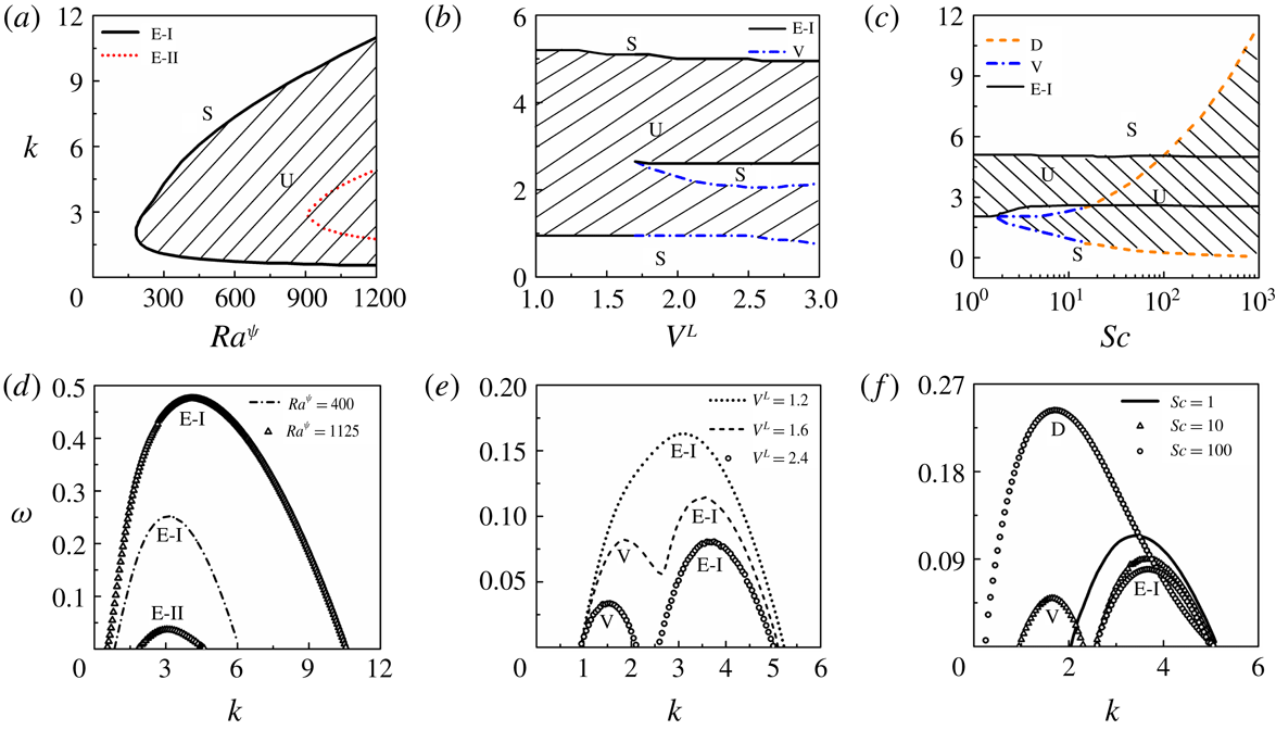
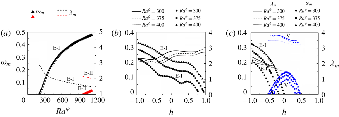
The literature discussed so far indicate that, while the contributions of inertial and molecular diffusive forces have been explored in detail in the past, arguably, there is no report as such of the influence of electric field induced instabilities on stratified two-layer miscible flows inside microchannels. In the present study, with the help of combined experimental as well as theoretical analyses, the effects of electroconvection on a two-layer viscosity stratified miscible flow inside a microchannel have been explored. We report the experimental investigations of the various regimes of instabilities produced due to ion injections from electrodes into a viscosity stratified flow of miscible fluids, which subsequently lead to the coherent mixing of the fluid streams. Experiments uncover three different instability regimes with an increase in electric field intensity, namely, a linear-onset regime, time-periodic nonlinear regime with the formation of von Kármán vortices and a chaotic flow regime. An Orr–Sommerfeld analysis of the governing equations with appropriate boundary conditions has also been performed to identify the various linear modes of instabilities of the system, which helps in the identification of the onset conditions of the EHD instabilities.
The paper is organized as follows. Section 2 contains a description of the experimental methodology, in § 3 the mathematical formulation is shown along with the linear stability equations, and solutions of the base states. Section 4 covers the experimental and theoretical results. Section 5 contains the conclusions from the analysis.
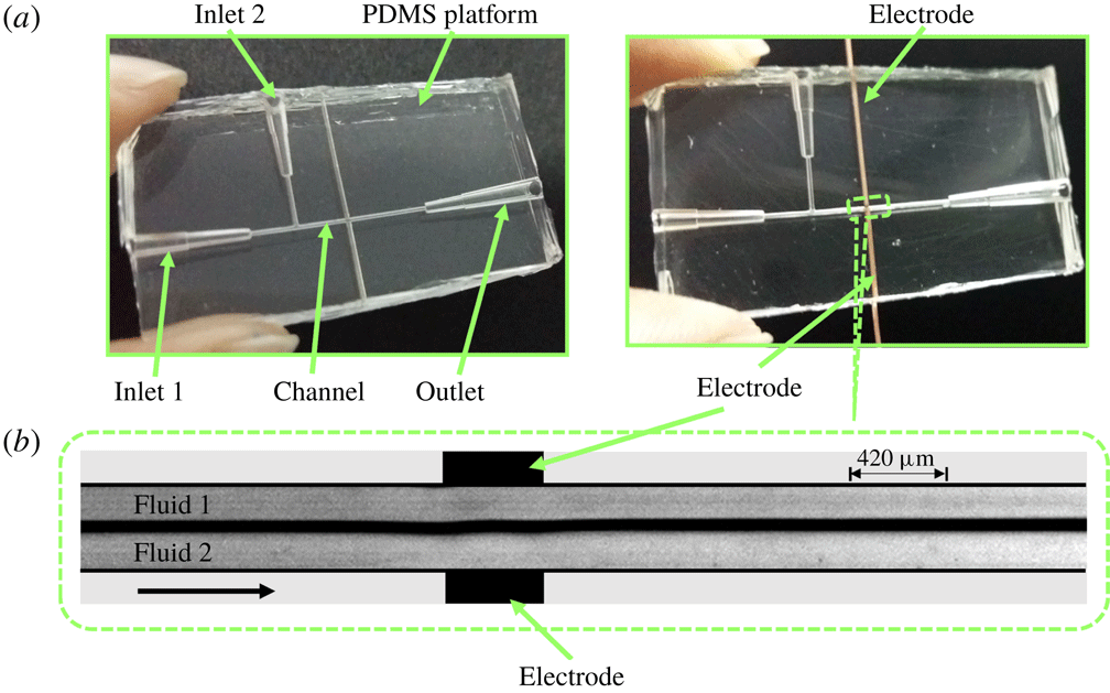
Figure 1. (a) Shows the top view of the experimental microchannel on a poly-dimethylsiloxane (PDMS) platform. Fluids 1 and 2 with viscosities
 $\unicode[STIX]{x1D707}_{1}$
and
$\unicode[STIX]{x1D707}_{1}$
and
 $\unicode[STIX]{x1D707}_{2}$
(
$\unicode[STIX]{x1D707}_{2}$
(
 $\unicode[STIX]{x1D707}_{2}>\unicode[STIX]{x1D707}_{1}$
), respectively, enter the channel through their respective inlets, and are then subjected to an electric field applied from a direct current (DC) high voltage source through Cu wire electrodes as shown. (b) Shows the experimental micrograph of the top view of the region marked in (a). Fluids 1 and 2 form a stratified flow in the channel (side by side), and are subjected to an electric field via Cu wire electrodes. The diameter of the channel and the electrodes are
$\unicode[STIX]{x1D707}_{2}>\unicode[STIX]{x1D707}_{1}$
), respectively, enter the channel through their respective inlets, and are then subjected to an electric field applied from a direct current (DC) high voltage source through Cu wire electrodes as shown. (b) Shows the experimental micrograph of the top view of the region marked in (a). Fluids 1 and 2 form a stratified flow in the channel (side by side), and are subjected to an electric field via Cu wire electrodes. The diameter of the channel and the electrodes are
 $420~\unicode[STIX]{x03BC}\text{m}$
. The average
$420~\unicode[STIX]{x03BC}\text{m}$
. The average
 $Re$
of the flow is maintained at 0.5. The arrow in (b) indicates the direction of the flow.
$Re$
of the flow is maintained at 0.5. The arrow in (b) indicates the direction of the flow.
2 Experiment
2.1 Materials and methods
Experiments were carried out in a cylindrical microchannel of
 $420~\unicode[STIX]{x03BC}\text{m}$
diameter built on a PDMS (poly-dimethylsiloxane) platform. The channels were fabricated by template moulding technique (Timung et al.
Reference Timung, Chaudhuri, Borthakur, Mandal, Biswas and Bandyopadhyay2017) employing a silicone elastomer (SLYGARD 184 silicone elastomer, Dow Corning). For the fabrication of the channels, templates were first prepared with the help of copper wires (Cu) of the same dimension, as required for the channel. A rectangular well was then formed with double sided tapes, with the Cu wire template fixed into the well. Liquid PDMS mixed with a cross-linker in the ratio
$420~\unicode[STIX]{x03BC}\text{m}$
diameter built on a PDMS (poly-dimethylsiloxane) platform. The channels were fabricated by template moulding technique (Timung et al.
Reference Timung, Chaudhuri, Borthakur, Mandal, Biswas and Bandyopadhyay2017) employing a silicone elastomer (SLYGARD 184 silicone elastomer, Dow Corning). For the fabrication of the channels, templates were first prepared with the help of copper wires (Cu) of the same dimension, as required for the channel. A rectangular well was then formed with double sided tapes, with the Cu wire template fixed into the well. Liquid PDMS mixed with a cross-linker in the ratio
 $10:1$
was then poured inside the well before curing the system in a vacuum oven at
$10:1$
was then poured inside the well before curing the system in a vacuum oven at
 $80\,^{\circ }\text{C}$
for 2 h. The template was then pulled out of the solid PDMS block to form the channels of required configuration. The Cu wire electrodes of
$80\,^{\circ }\text{C}$
for 2 h. The template was then pulled out of the solid PDMS block to form the channels of required configuration. The Cu wire electrodes of
 $420~\unicode[STIX]{x03BC}\text{m}$
diameter were integrated across the channel wall, for application of electric field potential. Experiments were conducted using different liquid pairs. Benzene (analytical grade, procured from Merck Ltd. (India), viscosity,
$420~\unicode[STIX]{x03BC}\text{m}$
diameter were integrated across the channel wall, for application of electric field potential. Experiments were conducted using different liquid pairs. Benzene (analytical grade, procured from Merck Ltd. (India), viscosity,
 $\unicode[STIX]{x1D707}_{1}\approx 0.603$
cP at
$\unicode[STIX]{x1D707}_{1}\approx 0.603$
cP at
 $25\,^{\circ }\text{C}$
; dielectric constant,
$25\,^{\circ }\text{C}$
; dielectric constant,
 $\unicode[STIX]{x1D700}_{r1}\approx 2.284$
(van der Maesen Reference van der Maesen1949)) formed the lower viscosity phase. Oleic acid (analytical grade, procured from Merck Ltd. (India), viscosity,
$\unicode[STIX]{x1D700}_{r1}\approx 2.284$
(van der Maesen Reference van der Maesen1949)) formed the lower viscosity phase. Oleic acid (analytical grade, procured from Merck Ltd. (India), viscosity,
 $\unicode[STIX]{x1D707}_{2}\approx 18$
cP at
$\unicode[STIX]{x1D707}_{2}\approx 18$
cP at
 $25\,^{\circ }\text{C}$
; dielectric constant,
$25\,^{\circ }\text{C}$
; dielectric constant,
 $\unicode[STIX]{x1D700}_{r2}\approx 2.32$
(de Sousa et al.
Reference de Sousa, Moreira, Shirsley, Nero and Alcantara2009)), silicone oil (analytical grade, procured from Merck Ltd. (India), viscosity,
$\unicode[STIX]{x1D700}_{r2}\approx 2.32$
(de Sousa et al.
Reference de Sousa, Moreira, Shirsley, Nero and Alcantara2009)), silicone oil (analytical grade, procured from Merck Ltd. (India), viscosity,
 $\unicode[STIX]{x1D707}_{2}\approx 317$
cP at
$\unicode[STIX]{x1D707}_{2}\approx 317$
cP at
 $25\,^{\circ }\text{C}$
; dielectric constant,
$25\,^{\circ }\text{C}$
; dielectric constant,
 $\unicode[STIX]{x1D700}_{r2}\approx 2.5$
(Ren, Wang & Huang Reference Ren, Wang and Huang2016)) and soybean oil (procured from local vendor, viscosity,
$\unicode[STIX]{x1D700}_{r2}\approx 2.5$
(Ren, Wang & Huang Reference Ren, Wang and Huang2016)) and soybean oil (procured from local vendor, viscosity,
 $\unicode[STIX]{x1D707}_{2}\approx 50$
cP at
$\unicode[STIX]{x1D707}_{2}\approx 50$
cP at
 $25\,^{\circ }\text{C}$
; dielectric constant,
$25\,^{\circ }\text{C}$
; dielectric constant,
 $\unicode[STIX]{x1D700}_{r2}\approx 3.3$
(Spohner Reference Spohner2016)) formed the higher viscosity phases. The viscosities of the liquids were measured using interfacial rheometer (Anton Paar, Physica MCR 301).
$\unicode[STIX]{x1D700}_{r2}\approx 3.3$
(Spohner Reference Spohner2016)) formed the higher viscosity phases. The viscosities of the liquids were measured using interfacial rheometer (Anton Paar, Physica MCR 301).
Figure 1(a) shows photographs of the experimental channel, before and after electrode integration. The two liquids flowed through the inlets 1 and 2 of the PDMS channel with the help of a syringe pump (Harvard Apparatus, PHD 2000). Electric field was applied from a high voltage direct current (DC) source (SES Instruments Pvt. Ltd, EHT-II) via Cu wire electrodes of
 $420~\unicode[STIX]{x03BC}\text{m}$
diameter as shown figure 1(a). The flow of the liquids through the channel was recorded with a high speed camera (Photron, Fastcam Mini UX-100). A picoammeter (SES Instruments Pvt. Ltd, Model DPM-111) was used to measure the electric current across the electrodes. Figure 1(b) demonstrates the experimental micrograph of the highlighted portion in figure 1(a), which shows the stratified flow of fluids 1 and 2 in absence of an electric field. Before and after every experiment the channels were first cleaned by ultra-sonication in an acetone bath for 10 min. It was followed by treatment with 10 %
$420~\unicode[STIX]{x03BC}\text{m}$
diameter as shown figure 1(a). The flow of the liquids through the channel was recorded with a high speed camera (Photron, Fastcam Mini UX-100). A picoammeter (SES Instruments Pvt. Ltd, Model DPM-111) was used to measure the electric current across the electrodes. Figure 1(b) demonstrates the experimental micrograph of the highlighted portion in figure 1(a), which shows the stratified flow of fluids 1 and 2 in absence of an electric field. Before and after every experiment the channels were first cleaned by ultra-sonication in an acetone bath for 10 min. It was followed by treatment with 10 %
 $V/V$
dilute piranha solution (
$V/V$
dilute piranha solution (
 $\text{H}_{2}\text{SO}_{4}:\text{H}_{2}\text{O}_{2},3:1$
) for 15 min. The channels were then repeatedly washed with deionized water (Merck Millipore, grade I), dried by blowing nitrogen gas, and kept in an air oven at
$\text{H}_{2}\text{SO}_{4}:\text{H}_{2}\text{O}_{2},3:1$
) for 15 min. The channels were then repeatedly washed with deionized water (Merck Millipore, grade I), dried by blowing nitrogen gas, and kept in an air oven at
 $70\,^{\circ }\text{C}$
for 20 min.
$70\,^{\circ }\text{C}$
for 20 min.
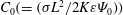
2.2 Calculation of injection level
Previous studies indicate that strong unipolar injections (
 $I^{q}\gg 1$
) with space charge limited currents can be achieved experimentally by covering the electrodes with suitable perm-selective membranes and varnishes (Atten & Gosse Reference Atten and Gosse1969; McCluskey & Atten Reference McCluskey and Atten1988). In comparison, for non-polar liquids, moderate and weak injections have been achieved by doping the liquids with appropriate salts (Denat et al.
Reference Denat, Gosse and Gosse1979; Pontiga, Castellanos & Malraison Reference Pontiga, Castellanos and Malraison1995). It has also been shown that intense localized injections of charge can be achieved by concentrating the electric field with the use of blade or needle electrodes (Tobazeon, Haidara & Atten Reference Tobazeon, Haidara and Atten1984; Atten & Haidara Reference Atten and Haidara1985; Higuera Reference Higuera2002; Tsukahara, Hirose & Otsubo Reference Tsukahara, Hirose and Otsubo2013). In the reported experiments, a DC voltage was applied from a high voltage source with the help of wire electrodes for the injection of charge into the dielectric experimental fluids. Since the electrodes were in contact with the experimental fluids, the injection of charge in the regions of high electric field was inevitable (Vasilkov, Chirkov & Stishkov Reference Vasilkov, Chirkov and Stishkov2017). In order to measure the injection level, a stratified flow of the lower viscosity phase, composed of benzene, and higher viscosity phase, composed of oleic acid (or silicone oil), was maintained in the microchannel with the help of a syringe pump. DC voltage input was applied to the system with the help of the copper wire electrodes, while the electric current was measured across the electrodes with the help of a picoammeter. The current–voltage curves for the cases: (i) benzene–oleic acid and (ii) benzene–silicone oil are shown in figure 2. The electric field intensity between the electrodes was obtained by dividing the applied voltage by the distance between the electrodes
$I^{q}\gg 1$
) with space charge limited currents can be achieved experimentally by covering the electrodes with suitable perm-selective membranes and varnishes (Atten & Gosse Reference Atten and Gosse1969; McCluskey & Atten Reference McCluskey and Atten1988). In comparison, for non-polar liquids, moderate and weak injections have been achieved by doping the liquids with appropriate salts (Denat et al.
Reference Denat, Gosse and Gosse1979; Pontiga, Castellanos & Malraison Reference Pontiga, Castellanos and Malraison1995). It has also been shown that intense localized injections of charge can be achieved by concentrating the electric field with the use of blade or needle electrodes (Tobazeon, Haidara & Atten Reference Tobazeon, Haidara and Atten1984; Atten & Haidara Reference Atten and Haidara1985; Higuera Reference Higuera2002; Tsukahara, Hirose & Otsubo Reference Tsukahara, Hirose and Otsubo2013). In the reported experiments, a DC voltage was applied from a high voltage source with the help of wire electrodes for the injection of charge into the dielectric experimental fluids. Since the electrodes were in contact with the experimental fluids, the injection of charge in the regions of high electric field was inevitable (Vasilkov, Chirkov & Stishkov Reference Vasilkov, Chirkov and Stishkov2017). In order to measure the injection level, a stratified flow of the lower viscosity phase, composed of benzene, and higher viscosity phase, composed of oleic acid (or silicone oil), was maintained in the microchannel with the help of a syringe pump. DC voltage input was applied to the system with the help of the copper wire electrodes, while the electric current was measured across the electrodes with the help of a picoammeter. The current–voltage curves for the cases: (i) benzene–oleic acid and (ii) benzene–silicone oil are shown in figure 2. The electric field intensity between the electrodes was obtained by dividing the applied voltage by the distance between the electrodes
 $(420~\unicode[STIX]{x03BC}\text{m})$
. The value of electric current across the electrodes was recorded for each applied voltage across each liquid separately before the same was repeated for the stratified flows. It has been shown in previous literature that for electric fields within the range
$(420~\unicode[STIX]{x03BC}\text{m})$
. The value of electric current across the electrodes was recorded for each applied voltage across each liquid separately before the same was repeated for the stratified flows. It has been shown in previous literature that for electric fields within the range
 $5\times 10^{2}\leqslant E\leqslant 5\times 10^{4}~\text{kV}~\text{cm}^{-1}$
, the charge density at the injector remains almost constant and independent of the electric field (Castellanos Reference Castellanos1991). Hence, the assumption of autonomous injection for the present analysis seems to be reasonably valid. The measured electrical current in the quiescent liquid is due to the contribution of two processes: (i) residual conduction and (ii) migration of injected ions (Denat et al.
Reference Denat, Gosse and Gosse1979; McCluskey et al.
Reference McCluskey, Atten and Perez1991). Previously, Denat et al. (Reference Denat, Gosse and Gosse1979) showed that the conduction current can be considered negligible if the ratio of conduction current to injection current,
$5\times 10^{2}\leqslant E\leqslant 5\times 10^{4}~\text{kV}~\text{cm}^{-1}$
, the charge density at the injector remains almost constant and independent of the electric field (Castellanos Reference Castellanos1991). Hence, the assumption of autonomous injection for the present analysis seems to be reasonably valid. The measured electrical current in the quiescent liquid is due to the contribution of two processes: (i) residual conduction and (ii) migration of injected ions (Denat et al.
Reference Denat, Gosse and Gosse1979; McCluskey et al.
Reference McCluskey, Atten and Perez1991). Previously, Denat et al. (Reference Denat, Gosse and Gosse1979) showed that the conduction current can be considered negligible if the ratio of conduction current to injection current,
 $C_{0}(=(\unicode[STIX]{x1D70E}L^{2}/2K\unicode[STIX]{x1D700}\unicode[STIX]{x1D6F9}_{0}))$
, is less than 0.5. The working liquids benzene and oleic (or silicone oil) acid have conductivities of the order of
$C_{0}(=(\unicode[STIX]{x1D70E}L^{2}/2K\unicode[STIX]{x1D700}\unicode[STIX]{x1D6F9}_{0}))$
, is less than 0.5. The working liquids benzene and oleic (or silicone oil) acid have conductivities of the order of
 ${\sim}10^{-13}~\text{Sm}^{-1}$
(Bobyl, Romanets & Alyab’ev Reference Bobyl, Romanets and Alyab’ev1965; Zhang, Edirisinghe & Jayasinghe Reference Zhang, Edirisinghe and Jayasinghe2006), while the value of ionic mobility
${\sim}10^{-13}~\text{Sm}^{-1}$
(Bobyl, Romanets & Alyab’ev Reference Bobyl, Romanets and Alyab’ev1965; Zhang, Edirisinghe & Jayasinghe Reference Zhang, Edirisinghe and Jayasinghe2006), while the value of ionic mobility
 $K$
in the working liquids is of the order of
$K$
in the working liquids is of the order of
 ${\sim}(10^{-8}{-}10^{-10})~\text{m}^{2}~\text{s}^{-1}~\text{V}^{-1}$
(Denat et al.
Reference Denat, Gosse and Gosse1979). In such a situation, the value of
${\sim}(10^{-8}{-}10^{-10})~\text{m}^{2}~\text{s}^{-1}~\text{V}^{-1}$
(Denat et al.
Reference Denat, Gosse and Gosse1979). In such a situation, the value of
 $C_{0}$
was found to be less than 0.5 for the experiments reported in the present work. Thus, the total current was considered to be due to ionic injections from the electrodes only. Thereafter, the injection level
$C_{0}$
was found to be less than 0.5 for the experiments reported in the present work. Thus, the total current was considered to be due to ionic injections from the electrodes only. Thereafter, the injection level
 $I^{q}$
was calculated from (3.9), using the current voltage curves shown in figure 2. The injection levels
$I^{q}$
was calculated from (3.9), using the current voltage curves shown in figure 2. The injection levels
 $I^{q}$
for the experiments shown in the present study were found to be in the range of 0.5–1.15, indicating a moderate injection.
$I^{q}$
for the experiments shown in the present study were found to be in the range of 0.5–1.15, indicating a moderate injection.
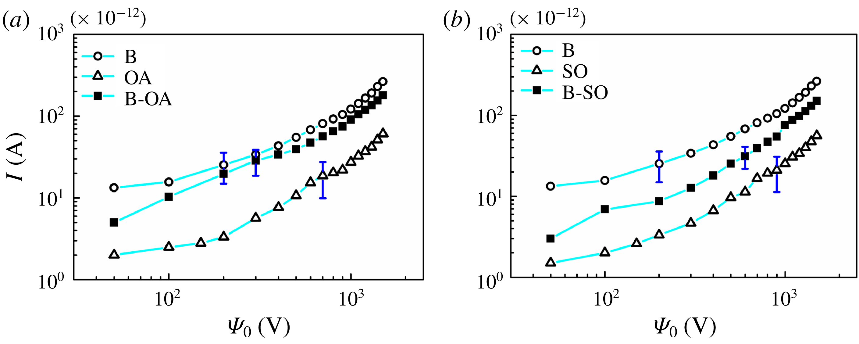
Figure 2. (a,b
) Show the current
 $(I)$
versus voltage (
$(I)$
versus voltage (
 $\unicode[STIX]{x1D6F9}_{0}$
) curves for different combinations of flows. (a) Shows the combination of single component flows of benzene (B), oleic acid (OA) and a stratified flow of benzene and oleic acid (B-OA). (b) Shows the combination of single component flows of benzene (B), silicone oil (SO) and a stratified flow of benzene and silicone oil (B-SO). The error bar represents the maximum standard deviation obtained from three experiments.
$\unicode[STIX]{x1D6F9}_{0}$
) curves for different combinations of flows. (a) Shows the combination of single component flows of benzene (B), oleic acid (OA) and a stratified flow of benzene and oleic acid (B-OA). (b) Shows the combination of single component flows of benzene (B), silicone oil (SO) and a stratified flow of benzene and silicone oil (B-SO). The error bar represents the maximum standard deviation obtained from three experiments.
3 Theoretical formulation
3.1 Problem formulation
The experiments were carried out in a cylindrical microchannel (
 $420~\unicode[STIX]{x03BC}\text{m}$
diameter) as already discussed in § 2.1. To gain in-depth information about the nature and onset conditions of the reported EHD instabilities, a scrupulous investigation considering a similar flow geometry to the experimental channel is required. However, the mathematical treatment of the problem considering a cylindrical coordinate system is seemingly cumbersome, especially because the experimental flow configuration is non-axisymmetric, due to integration of the electrodes on the channel walls. This calls for a complete three-dimensional formulation of the problem in the cylindrical coordinate system followed by a global stability analysis, which in the context of the reported problem will be extremely involved. We thus resorted to a two-dimensional planar geometry. Figure 3(a) depicts the laminar flow of a pair of miscible fluids flowing through a channel, before being subjected to a DC voltage
$420~\unicode[STIX]{x03BC}\text{m}$
diameter) as already discussed in § 2.1. To gain in-depth information about the nature and onset conditions of the reported EHD instabilities, a scrupulous investigation considering a similar flow geometry to the experimental channel is required. However, the mathematical treatment of the problem considering a cylindrical coordinate system is seemingly cumbersome, especially because the experimental flow configuration is non-axisymmetric, due to integration of the electrodes on the channel walls. This calls for a complete three-dimensional formulation of the problem in the cylindrical coordinate system followed by a global stability analysis, which in the context of the reported problem will be extremely involved. We thus resorted to a two-dimensional planar geometry. Figure 3(a) depicts the laminar flow of a pair of miscible fluids flowing through a channel, before being subjected to a DC voltage
 $\unicode[STIX]{x1D6F9}_{0}$
. A Cartesian coordinate system is chosen as the reference frame with the
$\unicode[STIX]{x1D6F9}_{0}$
. A Cartesian coordinate system is chosen as the reference frame with the
 $x$
and
$x$
and
 $z$
axes perpendicular to each other on the same plane. The distance between the two electrodes is 2
$z$
axes perpendicular to each other on the same plane. The distance between the two electrodes is 2
 $R$
, while the electric field is applied in the
$R$
, while the electric field is applied in the
 $z$
direction. The fluids, namely, fluid 1 of viscosity
$z$
direction. The fluids, namely, fluid 1 of viscosity
 $\unicode[STIX]{x1D707}_{1}$
and fluid 2 of viscosity
$\unicode[STIX]{x1D707}_{1}$
and fluid 2 of viscosity
 $\unicode[STIX]{x1D707}_{2}$
(
$\unicode[STIX]{x1D707}_{2}$
(
 $\unicode[STIX]{x1D707}_{2}>\unicode[STIX]{x1D707}_{1}$
), are assumed to be of equal density, and dielectric permittivity, and the ionic mobility is considered to be the same in both fluids. For two miscible fluids flowing inside a microchannel, the associated mass transfer Péclet number
$\unicode[STIX]{x1D707}_{2}>\unicode[STIX]{x1D707}_{1}$
), are assumed to be of equal density, and dielectric permittivity, and the ionic mobility is considered to be the same in both fluids. For two miscible fluids flowing inside a microchannel, the associated mass transfer Péclet number
 $[Pe=ul/\unicode[STIX]{x1D705}]$
, is of the order of
$[Pe=ul/\unicode[STIX]{x1D705}]$
, is of the order of
 ${\sim}10^{2}$
or higher (Stroock et al.
Reference Stroock, Dertinger, Ajdari, Mezić, Stone and Whitesides2002), leading to a slow diffusive mixing between the fluids. Thus, in the present study, which is motivated by flows inside microchannels, the thickness of the mixed interface can be effectively assumed to be constant. The interface between the two fluids grows diffusively to a distance
${\sim}10^{2}$
or higher (Stroock et al.
Reference Stroock, Dertinger, Ajdari, Mezić, Stone and Whitesides2002), leading to a slow diffusive mixing between the fluids. Thus, in the present study, which is motivated by flows inside microchannels, the thickness of the mixed interface can be effectively assumed to be constant. The interface between the two fluids grows diffusively to a distance
 $\unicode[STIX]{x1D6FF}$
in such a manner that fluid 1 occupies the region
$\unicode[STIX]{x1D6FF}$
in such a manner that fluid 1 occupies the region
 $h+\unicode[STIX]{x1D6FF}/2\leqslant z\leqslant R$
and fluid 2 occupies the region
$h+\unicode[STIX]{x1D6FF}/2\leqslant z\leqslant R$
and fluid 2 occupies the region
 $-R\leqslant z\leqslant h-\unicode[STIX]{x1D6FF}/2$
, where
$-R\leqslant z\leqslant h-\unicode[STIX]{x1D6FF}/2$
, where
 $h$
is the distance of the mixed interface from the datum line
$h$
is the distance of the mixed interface from the datum line
 $z=0$
.
$z=0$
.
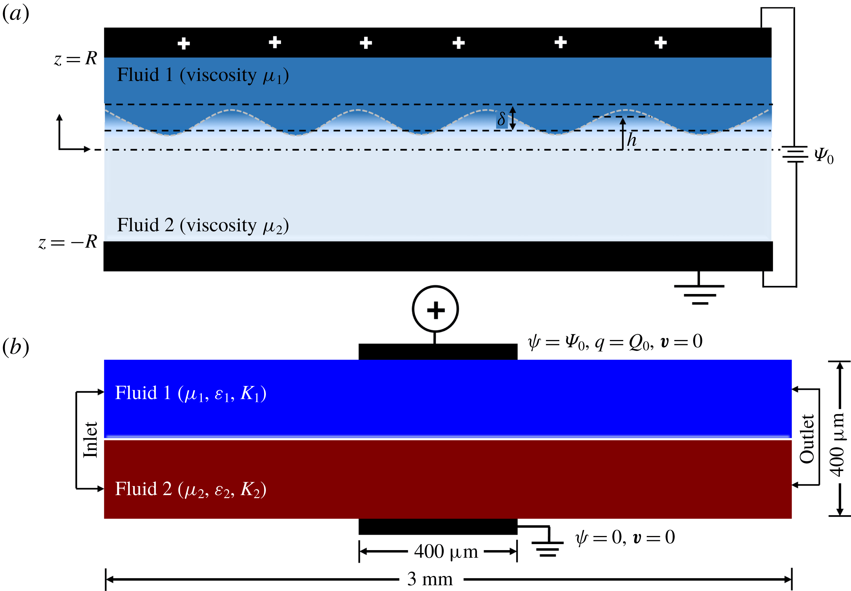
Figure 3. Schematic illustration of (a) the theoretical framework for the linear stability analysis. Two miscible fluids 1 and 2 with viscosities
 $\unicode[STIX]{x1D707}_{1}$
and
$\unicode[STIX]{x1D707}_{1}$
and
 $\unicode[STIX]{x1D707}_{2}$
(
$\unicode[STIX]{x1D707}_{2}$
(
 $\unicode[STIX]{x1D707}_{2}>\unicode[STIX]{x1D707}_{1}$
), respectively, form a stratified flow. The diffuse interface between them is of width
$\unicode[STIX]{x1D707}_{2}>\unicode[STIX]{x1D707}_{1}$
), respectively, form a stratified flow. The diffuse interface between them is of width
 $\unicode[STIX]{x1D6FF}$
, and located at a distance
$\unicode[STIX]{x1D6FF}$
, and located at a distance
 $h$
from the datum line,
$h$
from the datum line,
 $z=0$
. The fluids are subjected to an electric potential of
$z=0$
. The fluids are subjected to an electric potential of
 $\unicode[STIX]{x1D6F9}_{0}$
, applied through the electrodes separated by a distance of
$\unicode[STIX]{x1D6F9}_{0}$
, applied through the electrodes separated by a distance of
 $2R$
, where
$2R$
, where
 $R$
is half the channel width. (b) The computational domain for the nonlinear computational fluid dynamics (CFD) simulations.
$R$
is half the channel width. (b) The computational domain for the nonlinear computational fluid dynamics (CFD) simulations.
The viscosity of the fluids is formulated as an exponential function of the concentration scalar
 $S$
, such that the base values of the scalar
$S$
, such that the base values of the scalar
 $S_{0}$
are 0 and 1 in the top and bottom layers, respectively. The viscosity
$S_{0}$
are 0 and 1 in the top and bottom layers, respectively. The viscosity
 $\unicode[STIX]{x1D707}$
is modelled as,
$\unicode[STIX]{x1D707}$
is modelled as,
 $$\begin{eqnarray}\unicode[STIX]{x1D707}=\unicode[STIX]{x1D707}_{1}\exp (SV^{L}),\end{eqnarray}$$
where,
 $V^{L}$
is the log viscosity ratio of the fluids defined as,
$V^{L}$
is the log viscosity ratio of the fluids defined as,
 $V^{L}=\ln (\unicode[STIX]{x1D707}_{2}/\unicode[STIX]{x1D707}_{1})$
(Sahu & Govindarajan Reference Sahu and Govindarajan2016). The Reynolds number (
$V^{L}=\ln (\unicode[STIX]{x1D707}_{2}/\unicode[STIX]{x1D707}_{1})$
(Sahu & Govindarajan Reference Sahu and Govindarajan2016). The Reynolds number (
 $Re$
) is defined as
$Re$
) is defined as
 $Re=Q/R\unicode[STIX]{x1D702}_{1}$
, where
$Re=Q/R\unicode[STIX]{x1D702}_{1}$
, where
 $Q$
is the volumetric flow rate and
$Q$
is the volumetric flow rate and
 $\unicode[STIX]{x1D702}_{1}$
is the kinematic viscosity of fluid 1. In order to bring about homogeneity between the theoretical and experimental analyses, the strength of injection, characterized by the injection parameter,
$\unicode[STIX]{x1D702}_{1}$
is the kinematic viscosity of fluid 1. In order to bring about homogeneity between the theoretical and experimental analyses, the strength of injection, characterized by the injection parameter,
 $I^{q}$
, is calculated experimentally (refer to § 2.2), and used for the theoretical analysis. It is observed that the injection is homogeneous and autonomous in the experiments. Assuming a medium injection level, the value of the injection parameter,
$I^{q}$
, is calculated experimentally (refer to § 2.2), and used for the theoretical analysis. It is observed that the injection is homogeneous and autonomous in the experiments. Assuming a medium injection level, the value of the injection parameter,
 $I^{q}$
, is fixed at 1 for the theoretical analysis unless otherwise stated. In the formulation, ‘
$I^{q}$
, is fixed at 1 for the theoretical analysis unless otherwise stated. In the formulation, ‘
 $t$
’ represents time, the bold variables indicate vectors and the dashed variables denote derivative with respect to ‘
$t$
’ represents time, the bold variables indicate vectors and the dashed variables denote derivative with respect to ‘
 $z$
’.
$z$
’.
3.2 Governing equations
The fluids are assumed to be Newtonian and incompressible, thereby the flow field can be defined by the following continuity and momentum equations neglecting the effect of gravity,
 $$\begin{eqnarray}\displaystyle & \displaystyle \unicode[STIX]{x1D735}\boldsymbol{\cdot }\boldsymbol{v}=0, & \displaystyle\end{eqnarray}$$
 $$\begin{eqnarray}\displaystyle & \displaystyle \unicode[STIX]{x1D70C}\left(\frac{\unicode[STIX]{x2202}\boldsymbol{v}}{\unicode[STIX]{x2202}t}+\boldsymbol{v}\boldsymbol{\cdot }\unicode[STIX]{x1D735}\boldsymbol{v}\right)=-\unicode[STIX]{x1D735}p+\unicode[STIX]{x1D735}\boldsymbol{\cdot }[\unicode[STIX]{x1D707}(\unicode[STIX]{x1D735}\boldsymbol{v}+\unicode[STIX]{x1D735}\boldsymbol{v}^{\text{T}})]+\boldsymbol{F}_{\boldsymbol{ e}}. & \displaystyle\end{eqnarray}$$
Where
 $\boldsymbol{v}$
is the velocity vector,
$\boldsymbol{v}$
is the velocity vector,
 $\unicode[STIX]{x1D70C}$
is the density,
$\unicode[STIX]{x1D70C}$
is the density,
 $p$
is the pressure and
$p$
is the pressure and
 $\boldsymbol{F}_{\boldsymbol{e}}$
is the electrical body force term given by,
$\boldsymbol{F}_{\boldsymbol{e}}$
is the electrical body force term given by,
 $$\begin{eqnarray}\boldsymbol{F}_{\boldsymbol{e}}=q\boldsymbol{E}-\frac{1}{2}|\boldsymbol{E}|^{2}\unicode[STIX]{x1D735}\unicode[STIX]{x1D700}+\unicode[STIX]{x1D735}\left(\unicode[STIX]{x1D70C}\frac{|\boldsymbol{E}|^{2}}{2}\frac{\unicode[STIX]{x2202}\unicode[STIX]{x1D700}}{\unicode[STIX]{x2202}\unicode[STIX]{x1D70C}}\right).\end{eqnarray}$$
Here,
 $q$
represents the volumetric charge density,
$q$
represents the volumetric charge density,
 $\boldsymbol{E}$
is the electric field intensity and
$\boldsymbol{E}$
is the electric field intensity and
 $\unicode[STIX]{x1D700}$
is the electrical permittivity. The first term of (3.4) represents the Coulomb force exerted by the electric field on the free charges, and is generally the strongest in case of a DC supplied voltage. The second term of (3.4) is the dielectric force exerted by the electric field on the bound charges, and is neglected in the present analysis due to the negligible gradient of dielectric permittivity. The third term of (3.4) is the electrostrictive force which is included with the pressure term of the Navier–Stokes equation. The irrotational electric field
$\unicode[STIX]{x1D700}$
is the electrical permittivity. The first term of (3.4) represents the Coulomb force exerted by the electric field on the free charges, and is generally the strongest in case of a DC supplied voltage. The second term of (3.4) is the dielectric force exerted by the electric field on the bound charges, and is neglected in the present analysis due to the negligible gradient of dielectric permittivity. The third term of (3.4) is the electrostrictive force which is included with the pressure term of the Navier–Stokes equation. The irrotational electric field
 $\boldsymbol{E}$
is assumed to follow the field,
$\boldsymbol{E}$
is assumed to follow the field,
 $\boldsymbol{E}=-\unicode[STIX]{x1D735}\unicode[STIX]{x1D713}$
, which leads to the following Poisson’s equation originating from the governing Gauss’s law in which the electric field potential is defined as
$\boldsymbol{E}=-\unicode[STIX]{x1D735}\unicode[STIX]{x1D713}$
, which leads to the following Poisson’s equation originating from the governing Gauss’s law in which the electric field potential is defined as
 $\unicode[STIX]{x1D713}$
,
$\unicode[STIX]{x1D713}$
,
 $$\begin{eqnarray}\displaystyle & \displaystyle q=\unicode[STIX]{x1D735}\boldsymbol{\cdot }\unicode[STIX]{x1D700}\boldsymbol{E}, & \displaystyle\end{eqnarray}$$
 $$\begin{eqnarray}\displaystyle & \displaystyle \unicode[STIX]{x1D6FB}^{2}\unicode[STIX]{x1D713}=-\frac{q}{\unicode[STIX]{x1D700}}. & \displaystyle\end{eqnarray}$$
The continuity equation for charge density is given by,
 $$\begin{eqnarray}\frac{\unicode[STIX]{x2202}q}{\unicode[STIX]{x2202}t}+\unicode[STIX]{x1D735}\boldsymbol{\cdot }\boldsymbol{J}=0,\end{eqnarray}$$
where, the current density
 $\boldsymbol{J}$
is given by,
$\boldsymbol{J}$
is given by,
 $$\begin{eqnarray}\boldsymbol{J}=q\boldsymbol{v}+qK\boldsymbol{E}-D\unicode[STIX]{x1D735}q+\unicode[STIX]{x1D70E}\boldsymbol{E}.\end{eqnarray}$$
The first term of (3.8) accounts for the convection of charges due to motion of the fluid moving with a velocity
 $\boldsymbol{v}$
. The second term accounts for the drift transport of charges under the effect of the electric field, where
$\boldsymbol{v}$
. The second term accounts for the drift transport of charges under the effect of the electric field, where
 $K$
is the mobility of the ions moving with velocity
$K$
is the mobility of the ions moving with velocity
 $K\boldsymbol{E}$
. The third term accounts for the diffusive transport of the ions with diffusion coefficient
$K\boldsymbol{E}$
. The third term accounts for the diffusive transport of the ions with diffusion coefficient
 $D$
, which is neglected because of its smaller magnitude as compared to the other terms (Lacroix et al.
Reference Lacroix, Atten and Hopfinger1975; Denat et al.
Reference Denat, Gosse and Gosse1979; Castellanos Reference Castellanos1991). In the present analysis, the fluids under study are considered to be nearly electrically non-conductive (
$D$
, which is neglected because of its smaller magnitude as compared to the other terms (Lacroix et al.
Reference Lacroix, Atten and Hopfinger1975; Denat et al.
Reference Denat, Gosse and Gosse1979; Castellanos Reference Castellanos1991). In the present analysis, the fluids under study are considered to be nearly electrically non-conductive (
 $\unicode[STIX]{x1D70E}\leqslant 10^{-13}~\text{Sm}^{-1}$
), thereby making the last term of (3.8) negligible. Therefore, the constitutive relation for current density reduces to,
$\unicode[STIX]{x1D70E}\leqslant 10^{-13}~\text{Sm}^{-1}$
), thereby making the last term of (3.8) negligible. Therefore, the constitutive relation for current density reduces to,
 $$\begin{eqnarray}\boldsymbol{J}=q\boldsymbol{v}+qK\boldsymbol{E}.\end{eqnarray}$$
Substituting (3.9) into (3.7), and using (3.2), we obtain the conservation equation for the charge density as,
 $$\begin{eqnarray}\frac{\unicode[STIX]{x2202}q}{\unicode[STIX]{x2202}t}+\boldsymbol{v}\boldsymbol{\cdot }(\unicode[STIX]{x1D735}q)+K[q(\unicode[STIX]{x1D735}\boldsymbol{\cdot }\boldsymbol{E})+\boldsymbol{E}\boldsymbol{\cdot }(\unicode[STIX]{x1D735}q)]=0.\end{eqnarray}$$
The advection–diffusion equation for the concentration scalar
 $S$
gives,
$S$
gives,
 $$\begin{eqnarray}\frac{\unicode[STIX]{x2202}S}{\unicode[STIX]{x2202}t}+\boldsymbol{v}\boldsymbol{\cdot }\unicode[STIX]{x1D735}S=\unicode[STIX]{x1D705}\unicode[STIX]{x1D6FB}^{2}S.\end{eqnarray}$$
Here,
 $\unicode[STIX]{x1D705}$
is the diffusion coefficient of the scalar. For the velocity field, no-slip and no-penetration boundary conditions are enforced at the channel walls, i.e. [
$\unicode[STIX]{x1D705}$
is the diffusion coefficient of the scalar. For the velocity field, no-slip and no-penetration boundary conditions are enforced at the channel walls, i.e. [
 $\boldsymbol{v}(\pm R)=0,\boldsymbol{v}^{\prime }(\pm R)=0$
]. The boundary conditions used to solve for the electric potential
$\boldsymbol{v}(\pm R)=0,\boldsymbol{v}^{\prime }(\pm R)=0$
]. The boundary conditions used to solve for the electric potential
 $\unicode[STIX]{x1D713}$
are:
$\unicode[STIX]{x1D713}$
are:
 $\unicode[STIX]{x1D713}(R)=\unicode[STIX]{x1D6F9}_{0},\unicode[STIX]{x1D713}(-R)=0$
.
$\unicode[STIX]{x1D713}(R)=\unicode[STIX]{x1D6F9}_{0},\unicode[STIX]{x1D713}(-R)=0$
.
3.3 Non-dimensional governing equations
The equations are reduced to dimensionless forms by using the following scheme,
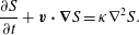
 $$\begin{eqnarray}\left.\begin{array}{@{}c@{}}\displaystyle (x,z,h,\unicode[STIX]{x1D6FF})=R(x^{\ast },z^{\ast },h^{\ast },\unicode[STIX]{x1D6FF}^{\ast }),\quad (u,\mathit{w})=\frac{K\unicode[STIX]{x1D6F9}_{0}}{R}(u^{\ast },w^{\ast }),\quad \unicode[STIX]{x1D713}=\unicode[STIX]{x1D6F9}_{0}\unicode[STIX]{x1D713}^{\ast },\\ \displaystyle q=Q_{0}q^{\ast },\quad t=\frac{R^{2}}{K\unicode[STIX]{x1D6F9}_{0}}t^{\ast },\quad p=\frac{\unicode[STIX]{x1D70C}K^{2}\unicode[STIX]{x1D6F9}_{0}^{2}}{R^{2}}p^{\ast },\quad \unicode[STIX]{x1D707}=\unicode[STIX]{x1D707}_{1}\unicode[STIX]{x1D707}^{\ast }.\end{array}\right\}\end{eqnarray}$$
The asterisk symbol depicts dimensionless quantities. Here,
 $\unicode[STIX]{x1D6F9}_{0}$
and
$\unicode[STIX]{x1D6F9}_{0}$
and
 $Q_{0}$
represent the applied voltage and the charge density at the injector, respectively. The dimensionless governing equations after dropping the asterisk symbol are,
$Q_{0}$
represent the applied voltage and the charge density at the injector, respectively. The dimensionless governing equations after dropping the asterisk symbol are,
 $$\begin{eqnarray}\displaystyle & \displaystyle \unicode[STIX]{x1D735}\boldsymbol{\cdot }\boldsymbol{v}=0, & \displaystyle\end{eqnarray}$$
 $$\begin{eqnarray}\displaystyle & \displaystyle \frac{\unicode[STIX]{x2202}\boldsymbol{v}}{\unicode[STIX]{x2202}t}+\boldsymbol{v}\boldsymbol{\cdot }\unicode[STIX]{x1D735}\boldsymbol{v}=-\unicode[STIX]{x1D735}p+\frac{1}{Re^{\unicode[STIX]{x1D713}}}\unicode[STIX]{x1D735}\boldsymbol{\cdot }[\unicode[STIX]{x1D707}(\unicode[STIX]{x1D735}\boldsymbol{v}+\unicode[STIX]{x1D735}\boldsymbol{v}^{\text{T}})]+I^{q}{R_{M}}^{2}(q\boldsymbol{E}), & \displaystyle\end{eqnarray}$$
 $$\begin{eqnarray}\displaystyle & \displaystyle \unicode[STIX]{x1D6FB}^{2}\unicode[STIX]{x1D713}=-I^{q}q, & \displaystyle\end{eqnarray}$$
 $$\begin{eqnarray}\displaystyle & \displaystyle \frac{\unicode[STIX]{x2202}q}{\unicode[STIX]{x2202}t}+\boldsymbol{v}\boldsymbol{\cdot }(\unicode[STIX]{x1D735}q)+q(\unicode[STIX]{x1D735}\boldsymbol{\cdot }\boldsymbol{E})+\boldsymbol{E}\boldsymbol{\cdot }(\unicode[STIX]{x1D735}q)=0, & \displaystyle\end{eqnarray}$$
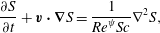 $$\begin{eqnarray}\displaystyle & \displaystyle \frac{\unicode[STIX]{x2202}S}{\unicode[STIX]{x2202}t}+\boldsymbol{v}\boldsymbol{\cdot }\unicode[STIX]{x1D735}S=\frac{1}{Re^{\unicode[STIX]{x1D713}}Sc}\unicode[STIX]{x1D6FB}^{2}S, & \displaystyle\end{eqnarray}$$
where,
 $$\begin{eqnarray}Re^{\unicode[STIX]{x1D713}}=\frac{K\unicode[STIX]{x1D6F9}_{0}}{\unicode[STIX]{x1D702}_{1}},\quad R_{M}=\frac{(\unicode[STIX]{x1D700}/\unicode[STIX]{x1D70C})^{1/2}}{K},\quad I^{q}=\frac{Q_{0}R^{2}}{\unicode[STIX]{x1D700}\unicode[STIX]{x1D6F9}_{0}},\quad Sc=\frac{\unicode[STIX]{x1D702}_{1}}{\unicode[STIX]{x1D705}}.\end{eqnarray}$$
Here,
 $Re^{\unicode[STIX]{x1D713}}$
is defined as the electric Reynolds number,
$Re^{\unicode[STIX]{x1D713}}$
is defined as the electric Reynolds number,
 $R_{M}$
is defined as the ratio between the hydrodynamic mobility
$R_{M}$
is defined as the ratio between the hydrodynamic mobility
 $[(\unicode[STIX]{x1D700}/\unicode[STIX]{x1D70C})^{1/2}]$
and the true ionic mobility
$[(\unicode[STIX]{x1D700}/\unicode[STIX]{x1D70C})^{1/2}]$
and the true ionic mobility
 $K$
,
$K$
,
 $I^{q}$
is the charge injection level and
$I^{q}$
is the charge injection level and
 $Sc$
is the Schmidt number. The electric field Rayleigh number
$Sc$
is the Schmidt number. The electric field Rayleigh number
 $Ra^{\unicode[STIX]{x1D713}}$
is defined as
$Ra^{\unicode[STIX]{x1D713}}$
is defined as
 $Ra^{\unicode[STIX]{x1D713}}=Re^{\unicode[STIX]{x1D713}}{R_{M}}^{2}=(\unicode[STIX]{x1D700}\unicode[STIX]{x1D6F9}_{0})/(\unicode[STIX]{x1D707}_{1}K)$
, and gives the ratio of the electrostatic to viscous force. The non-dimensional boundary conditions used to solve the velocity field are:
$Ra^{\unicode[STIX]{x1D713}}=Re^{\unicode[STIX]{x1D713}}{R_{M}}^{2}=(\unicode[STIX]{x1D700}\unicode[STIX]{x1D6F9}_{0})/(\unicode[STIX]{x1D707}_{1}K)$
, and gives the ratio of the electrostatic to viscous force. The non-dimensional boundary conditions used to solve the velocity field are:
 $\boldsymbol{v}(\pm 1)=0,\boldsymbol{v}^{\prime }(\pm 1)=0$
. For the solution of the electric potential
$\boldsymbol{v}(\pm 1)=0,\boldsymbol{v}^{\prime }(\pm 1)=0$
. For the solution of the electric potential
 $\unicode[STIX]{x1D713}$
, the non-dimensional boundary conditions used are:
$\unicode[STIX]{x1D713}$
, the non-dimensional boundary conditions used are:
 $\unicode[STIX]{x1D713}(1)=1,\unicode[STIX]{x1D713}(-1)=0$
,
$\unicode[STIX]{x1D713}(1)=1,\unicode[STIX]{x1D713}(-1)=0$
,
 $\unicode[STIX]{x1D713}^{\prime \prime }(1)=-I^{q}$
.
$\unicode[STIX]{x1D713}^{\prime \prime }(1)=-I^{q}$
.
3.4 Linear stability
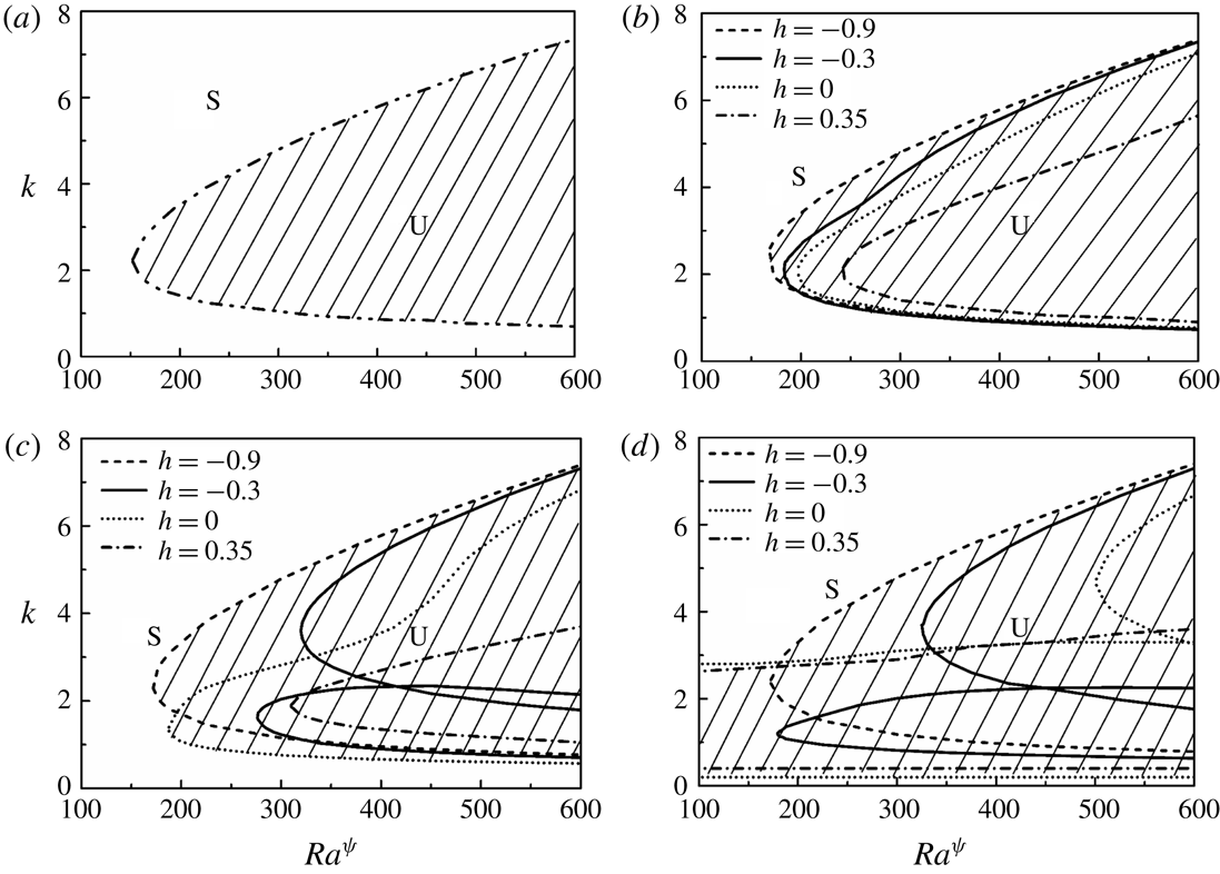
A general linear stability analysis (LSA) has been carried out by splitting the flow and electric field variables into base-state and perturbed-state quantities. We consider only the transverse modes because the existing literature suggests that the longitudinal modes remain unaffected by the parallel shear flow or the other parameters of interest reported in the present study (Castellanos & Agrait Reference Castellanos and Agrait1992; Lara, Castellanos & Pontiga Reference Lara, Castellanos and Pontiga1997; Sahu & Govindarajan Reference Sahu and Govindarajan2016). In such a scenario a two-dimensional (2-D) stability analysis is found to be sufficient to qualitatively uncover the underlying physics and predict the onset conditions. The formulation considering three-dimensional (3-D) perturbations is also shown in appendix B. The governing equations are linearized considering the following linear modes:
 $$\begin{eqnarray}\displaystyle [u,w,p,\unicode[STIX]{x1D713},S,\unicode[STIX]{x1D707}](x,z,t) & = & \displaystyle [u_{0}(z),0,p_{0},\unicode[STIX]{x1D713}_{0}(z),S_{0}(z),\unicode[STIX]{x1D707}_{0}(z)]\nonumber\\ \displaystyle & & \displaystyle +\,[\tilde{u} ,\tilde{w},\tilde{p},\tilde{\unicode[STIX]{x1D713}},\tilde{S},\tilde{\unicode[STIX]{x1D707}}](z)\text{e}^{(\unicode[STIX]{x1D714}t+\text{i}kx)}.\end{eqnarray}$$
The variables with subscript ‘0’ denote the base-state quantities and the variables with ‘tilde’ are the perturbed quantities. Here,
 $u$
and
$u$
and
 $w$
are the
$w$
are the
 $x$
and
$x$
and
 $z$
directional velocities, respectively. The symbols
$z$
directional velocities, respectively. The symbols
 $\unicode[STIX]{x1D714}$
and
$\unicode[STIX]{x1D714}$
and
 $k$
are the growth coefficient and the wavenumber of the perturbation, respectively. The parameter
$k$
are the growth coefficient and the wavenumber of the perturbation, respectively. The parameter
 $\unicode[STIX]{x1D714}$
is a complex quantity (
$\unicode[STIX]{x1D714}$
is a complex quantity (
 $\unicode[STIX]{x1D714}=\unicode[STIX]{x1D714}_{r}+\text{i}\unicode[STIX]{x1D714}_{i}$
). A perturbation is unstable when
$\unicode[STIX]{x1D714}=\unicode[STIX]{x1D714}_{r}+\text{i}\unicode[STIX]{x1D714}_{i}$
). A perturbation is unstable when
 $\unicode[STIX]{x1D714}_{r}>0$
, stable when
$\unicode[STIX]{x1D714}_{r}>0$
, stable when
 $\unicode[STIX]{x1D714}_{r}<0$
, and neutrally stable when
$\unicode[STIX]{x1D714}_{r}<0$
, and neutrally stable when
 $\unicode[STIX]{x1D714}_{r}=0$
. The perturbation viscosity
$\unicode[STIX]{x1D714}_{r}=0$
. The perturbation viscosity
 $\tilde{\unicode[STIX]{x1D707}}$
is modelled as,
$\tilde{\unicode[STIX]{x1D707}}$
is modelled as,
 $\tilde{\unicode[STIX]{x1D707}}=(\text{d}\unicode[STIX]{x1D707}_{0}/\text{d}S_{0})\tilde{S}$
(Sahu & Govindarajan Reference Sahu and Govindarajan2016).
$\tilde{\unicode[STIX]{x1D707}}=(\text{d}\unicode[STIX]{x1D707}_{0}/\text{d}S_{0})\tilde{S}$
(Sahu & Govindarajan Reference Sahu and Govindarajan2016).
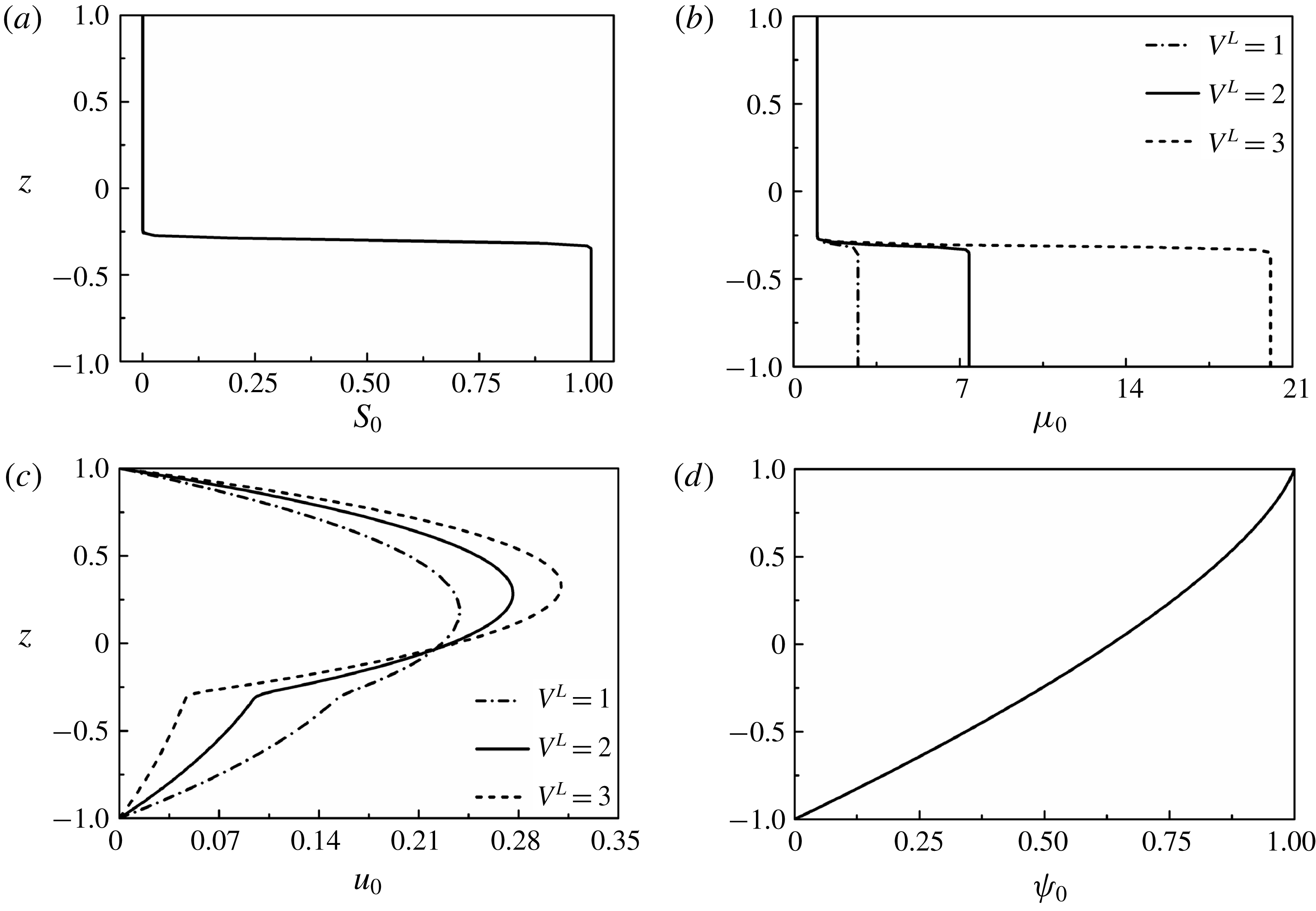
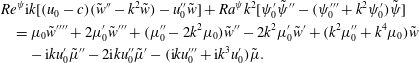
Figure 4. Base-state profiles for (a) concentration scalar
 $S_{0}$
, (b) viscosity
$S_{0}$
, (b) viscosity
 $\unicode[STIX]{x1D707}_{0}$
, (c) velocity
$\unicode[STIX]{x1D707}_{0}$
, (c) velocity
 $u_{0}$
and (d) potential
$u_{0}$
and (d) potential
 $\unicode[STIX]{x1D713}_{0}$
, for
$\unicode[STIX]{x1D713}_{0}$
, for
 $h=-0.3$
and
$h=-0.3$
and
 $\unicode[STIX]{x1D6FF}=0.02$
.
$\unicode[STIX]{x1D6FF}=0.02$
.
3.4.1 Base-state analysis
It is assumed that the diffusive interface between the two miscible fluids is of thickness
 $\unicode[STIX]{x1D6FF}$
. If
$\unicode[STIX]{x1D6FF}$
. If
 $\unicode[STIX]{x1D6FF}\ll 1$
, then the base-state profile of the concentration scalar can be estimated following a quasi-steady approximation
$\unicode[STIX]{x1D6FF}\ll 1$
, then the base-state profile of the concentration scalar can be estimated following a quasi-steady approximation
 $[\unicode[STIX]{x1D714}\gg \unicode[STIX]{x1D705}/\unicode[STIX]{x1D6FF}^{2}]$
(Tan & Homsy Reference Tan and Homsy1986; Selvam et al.
Reference Selvam, Merk, Govindarajan and Meiburg2007) as,
$[\unicode[STIX]{x1D714}\gg \unicode[STIX]{x1D705}/\unicode[STIX]{x1D6FF}^{2}]$
(Tan & Homsy Reference Tan and Homsy1986; Selvam et al.
Reference Selvam, Merk, Govindarajan and Meiburg2007) as,
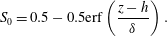 $$\begin{eqnarray}S_{0}=0.5-0.5\text{erf}\left(\frac{z-h}{\unicode[STIX]{x1D6FF}}\right).\end{eqnarray}$$
Here, the variable,
 $h$
, is the dimensionless distance of the diffused interface from the datum,
$h$
, is the dimensionless distance of the diffused interface from the datum,
 $z=0$
. The base-state profile of the concentration scalar is shown in figure 4(a). The base-state profiles for viscosity
$z=0$
. The base-state profile of the concentration scalar is shown in figure 4(a). The base-state profiles for viscosity
 $\unicode[STIX]{x1D707}_{0}$
, are then obtained from the relation,
$\unicode[STIX]{x1D707}_{0}$
, are then obtained from the relation,
 $$\begin{eqnarray}\unicode[STIX]{x1D707}_{0}=\exp (S_{0}V^{L}).\end{eqnarray}$$
The base-state velocity profile
 $u_{0}$
is then obtained by solving (3.14) for steady state, after dropping the electrical body force term, which gives,
$u_{0}$
is then obtained by solving (3.14) for steady state, after dropping the electrical body force term, which gives,
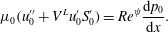 $$\begin{eqnarray}\unicode[STIX]{x1D707}_{0}(u_{0}^{\prime \prime }+V^{L}u_{0}^{\prime }S_{0}^{\prime })=Re^{\unicode[STIX]{x1D713}}\frac{\text{d}p_{0}}{\text{d}x}.\end{eqnarray}$$
Equation (3.22) is solved with no-slip boundary conditions at the channel walls,
 $u_{0}(\pm 1)=0$
, in which the non-dimensional pressure gradient,
$u_{0}(\pm 1)=0$
, in which the non-dimensional pressure gradient,
 $(\text{d}p_{0}/\text{d}x)$
, is fixed by assuming a constant volumetric flow rate. From (3.16) the base state equation for electric potential is obtained as,
$(\text{d}p_{0}/\text{d}x)$
, is fixed by assuming a constant volumetric flow rate. From (3.16) the base state equation for electric potential is obtained as,
 $$\begin{eqnarray}(\unicode[STIX]{x1D713}_{0}^{\prime \prime })^{2}+\unicode[STIX]{x1D713}_{0}^{\prime }\unicode[STIX]{x1D713}_{0}^{\prime \prime \prime }=0.\end{eqnarray}$$
Equation (3.23) is solved numerically with the boundary conditions: [
 $\unicode[STIX]{x1D713}_{0}(1)=1;\unicode[STIX]{x1D713}_{0}(-1)=0;\unicode[STIX]{x1D713}_{0}^{\prime \prime }(1)=-I^{q}$
]. The base-state profiles for viscosity (
$\unicode[STIX]{x1D713}_{0}(1)=1;\unicode[STIX]{x1D713}_{0}(-1)=0;\unicode[STIX]{x1D713}_{0}^{\prime \prime }(1)=-I^{q}$
]. The base-state profiles for viscosity (
 $\unicode[STIX]{x1D707}_{0}$
), velocity (
$\unicode[STIX]{x1D707}_{0}$
), velocity (
 $u_{0}$
) and electric potential (
$u_{0}$
) and electric potential (
 $\unicode[STIX]{x1D713}_{0}$
) are shown in figure 4(a–d). Panel (a) of this figure shows that
$\unicode[STIX]{x1D713}_{0}$
) are shown in figure 4(a–d). Panel (a) of this figure shows that
 $S_{0}$
is zero at layer 1 and it is one at layer 2 while the variation across the diffused interface is sharp but continuous. A similar trend of the variation in the dimensionless viscosity
$S_{0}$
is zero at layer 1 and it is one at layer 2 while the variation across the diffused interface is sharp but continuous. A similar trend of the variation in the dimensionless viscosity
 $\unicode[STIX]{x1D707}_{0}$
can also be seen in (b). Further, (c) shows the dimensionless velocity profile
$\unicode[STIX]{x1D707}_{0}$
can also be seen in (b). Further, (c) shows the dimensionless velocity profile
 $u_{0}$
of the base state under varied conditions. Panel (d) shows the variation of the base-state electric field potential,
$u_{0}$
of the base state under varied conditions. Panel (d) shows the variation of the base-state electric field potential,
 $\unicode[STIX]{x1D713}_{0}$
, across the fluid layers.
$\unicode[STIX]{x1D713}_{0}$
, across the fluid layers.
3.4.2 Perturbed-state analysis
The governing equations (3.13)–(3.17) are perturbed with the variables mentioned in (3.19) in which the growth coefficient,
 $\unicode[STIX]{x1D714}$
, is represented in terms of the wave speed
$\unicode[STIX]{x1D714}$
, is represented in terms of the wave speed
 $c$
as,
$c$
as,
 $\unicode[STIX]{x1D714}=-\text{i}kc$
. The dimensionless linearized equations of motion and continuity equation after eliminating the pressure perturbation term are given by,
$\unicode[STIX]{x1D714}=-\text{i}kc$
. The dimensionless linearized equations of motion and continuity equation after eliminating the pressure perturbation term are given by,
 $$\begin{eqnarray}\displaystyle & & \displaystyle Re^{\unicode[STIX]{x1D713}}\text{i}k[(u_{0}-c)(\tilde{w}^{\prime \prime }-k^{2}\tilde{w})-u_{0}^{\prime \prime }\tilde{w}]+Ra^{\unicode[STIX]{x1D713}}k^{2}[\unicode[STIX]{x1D713}_{0}^{\prime }\tilde{\unicode[STIX]{x1D713}}^{\prime \prime }-(\unicode[STIX]{x1D713}_{0}^{\prime \prime \prime }+k^{2}\unicode[STIX]{x1D713}_{0}^{\prime })\tilde{\unicode[STIX]{x1D713}}]\nonumber\\ \displaystyle & & \displaystyle \quad =\unicode[STIX]{x1D707}_{0}\tilde{w}^{\prime \prime \prime \prime }+2\unicode[STIX]{x1D707}_{0}^{\prime }\tilde{w}^{\prime \prime \prime }+(\unicode[STIX]{x1D707}_{0}^{\prime \prime }-2k^{2}\unicode[STIX]{x1D707}_{0})\tilde{w}^{\prime \prime }-2k^{2}\unicode[STIX]{x1D707}_{0}^{\prime }\tilde{w}^{\prime }+(k^{2}\unicode[STIX]{x1D707}_{0}^{\prime \prime }+k^{4}\unicode[STIX]{x1D707}_{0})\tilde{w}\nonumber\\ \displaystyle & & \displaystyle \qquad -\,\text{i}ku_{0}^{\prime }\tilde{\unicode[STIX]{x1D707}}^{\prime \prime }-2\text{i}ku_{0}^{\prime \prime }\tilde{\unicode[STIX]{x1D707}}^{\prime }-(\text{i}ku_{0}^{\prime \prime \prime }+\text{i}k^{3}u_{0}^{\prime })\tilde{\unicode[STIX]{x1D707}}.\end{eqnarray}$$
Equations (3.16) and (3.17) reduce to the following equations,
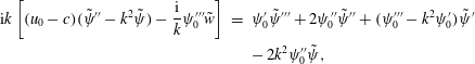 $$\begin{eqnarray}\displaystyle \text{i}k\left[(u_{0}-c)(\tilde{\unicode[STIX]{x1D713}}^{\prime \prime }-k^{2}\tilde{\unicode[STIX]{x1D713}})-\frac{\text{i}}{k}\unicode[STIX]{x1D713}_{0}^{\prime \prime \prime }\tilde{w}\right] & = & \displaystyle \unicode[STIX]{x1D713}_{0}^{\prime }\tilde{\unicode[STIX]{x1D713}}^{\prime \prime \prime }+2\unicode[STIX]{x1D713}_{0}^{\prime \prime }\tilde{\unicode[STIX]{x1D713}}^{\prime \prime }+(\unicode[STIX]{x1D713}_{0}^{\prime \prime \prime }-k^{2}\unicode[STIX]{x1D713}_{0}^{\prime })\tilde{\unicode[STIX]{x1D713}}^{\prime }\nonumber\\ \displaystyle & & \displaystyle -\,2k^{2}\unicode[STIX]{x1D713}_{0}^{\prime \prime }\tilde{\unicode[STIX]{x1D713}},\end{eqnarray}$$
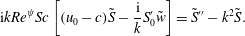 $$\begin{eqnarray}\text{i}kRe^{\unicode[STIX]{x1D713}}Sc\left[(u_{0}-c)\tilde{S}-\frac{\text{i}}{k}S_{0}^{\prime }\tilde{w}\right]=\tilde{S}^{\prime \prime }-k^{2}\tilde{S}.\end{eqnarray}$$
The boundary conditions employed to solve (3.24)–(3.26) are,
 $$\begin{eqnarray}\tilde{w}(\pm 1)=0,\quad \tilde{w}^{\prime }(\pm 1)=0,\end{eqnarray}$$
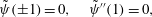 $$\begin{eqnarray}\tilde{\unicode[STIX]{x1D713}}(\pm 1)=0,\quad \tilde{\unicode[STIX]{x1D713}}^{\prime \prime }(1)=0,\end{eqnarray}$$
 $$\begin{eqnarray}\tilde{S}^{\prime }(\pm 1)=0.\end{eqnarray}$$
3.4.3 Numerical method
The domain is discretized employing a spectral collocation method based on Chebyshev polynomials (Orszag Reference Orszag1971; Weideman & Reddy Reference Weideman and Reddy2000). The three ordinary differential equations defined by (3.24)–(3.26) reduce to the following eigenvalue form upon discretization,
 $$\begin{eqnarray}\unicode[STIX]{x1D63C}\tilde{\unicode[STIX]{x1D719}}=\unicode[STIX]{x1D714}\unicode[STIX]{x1D63D}\tilde{\unicode[STIX]{x1D719}},\end{eqnarray}$$
where
 $\unicode[STIX]{x1D63C}$
and
$\unicode[STIX]{x1D63C}$
and
 $\unicode[STIX]{x1D63D}$
are
$\unicode[STIX]{x1D63D}$
are
 $3\times 3$
matrices, given by,
$3\times 3$
matrices, given by,
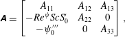 $$\begin{eqnarray}\displaystyle & \displaystyle \unicode[STIX]{x1D63C}=\left[\begin{array}{@{}ccc@{}}A_{11} & A_{12} & A_{13}\\ -Re^{\unicode[STIX]{x1D713}}ScS_{0}^{\prime } & A_{22} & 0\\ -\unicode[STIX]{x1D713}_{0}^{\prime \prime \prime } & 0 & A_{33}\\ \end{array}\right], & \displaystyle\end{eqnarray}$$
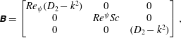 $$\begin{eqnarray}\displaystyle & \displaystyle \unicode[STIX]{x1D63D}=\left[\begin{array}{@{}ccc@{}}Re_{\unicode[STIX]{x1D713}}(D_{2}-k^{2}) & 0 & 0\\ 0 & Re^{\unicode[STIX]{x1D713}}Sc & 0\\ 0 & 0 & (D_{2}-k^{2})\\ \end{array}\right], & \displaystyle\end{eqnarray}$$
and,
 $$\begin{eqnarray}\displaystyle & \displaystyle \tilde{\unicode[STIX]{x1D719}}=\left[\begin{array}{@{}c@{}}\tilde{w}\\ \tilde{S}\\ \tilde{\unicode[STIX]{x1D713}}\\ \end{array}\right]. & \displaystyle\end{eqnarray}$$
Here,
 $D_{1}=\text{d}/\text{d}z$
,
$D_{1}=\text{d}/\text{d}z$
,
 $D_{2}=\text{d}^{2}/\text{d}z^{2}$
,
$D_{2}=\text{d}^{2}/\text{d}z^{2}$
,
 $D_{3}=\text{d}^{3}/\text{d}z^{3}$
,
$D_{3}=\text{d}^{3}/\text{d}z^{3}$
,
 $D_{4}=\text{d}^{4}/\text{d}z^{4}$
and
$D_{4}=\text{d}^{4}/\text{d}z^{4}$
and
 $$\begin{eqnarray}\left.\begin{array}{@{}c@{}}\displaystyle \begin{array}{@{}rcl@{}}\displaystyle A_{11}\; & =\; & \displaystyle \unicode[STIX]{x1D707}_{0}D_{4}+2\unicode[STIX]{x1D707}_{0}^{\prime }D_{3}+(\unicode[STIX]{x1D707}_{0}^{\prime \prime }-\text{i}kRe^{\unicode[STIX]{x1D713}}u_{0}-2k^{2}\unicode[STIX]{x1D707}_{0})D_{2}-2k^{2}\unicode[STIX]{x1D707}_{0}^{\prime }D_{1}\\ \; & \; & +\,\displaystyle \text{i}k\left(Re^{\unicode[STIX]{x1D713}}u_{0}^{\prime \prime }+\frac{k}{\text{i}}\unicode[STIX]{x1D707}_{0}^{\prime \prime }+Re^{\unicode[STIX]{x1D713}}k^{2}u_{0}+\frac{k^{3}}{\text{i}}\unicode[STIX]{x1D707}_{0}\right),\end{array}\\ \displaystyle \begin{array}{@{}rcl@{}}\displaystyle A_{12}\; & =\; & \displaystyle -\text{i}kV^{L}\unicode[STIX]{x1D707}_{0}u_{0}^{\prime }D_{2}-2\text{i}kV^{L}(\unicode[STIX]{x1D707}_{0}u_{0}^{\prime \prime }+u_{0}^{\prime }\unicode[STIX]{x1D707}_{0}^{\prime })D_{1}\\ \; & \; & -\,\text{i}kV^{L}(\unicode[STIX]{x1D707}_{0}u_{0}^{\prime \prime \prime }+k^{2}\unicode[STIX]{x1D707}_{0}u_{0}^{\prime }+u_{0}^{\prime }\unicode[STIX]{x1D707}_{0}^{\prime \prime }+2u_{0}^{\prime \prime }\unicode[STIX]{x1D707}_{0}^{\prime }),\end{array}\\ \displaystyle A_{13}=Ra^{\unicode[STIX]{x1D713}}k^{2}(\unicode[STIX]{x1D713}_{0}^{\prime \prime \prime }+k^{2}\unicode[STIX]{x1D713}_{0}^{\prime }-\unicode[STIX]{x1D713}_{0}^{\prime }D_{2}),\\ \displaystyle A_{22}=D_{2}-k^{2}-\text{i}kRe^{\unicode[STIX]{x1D713}}Scu_{0},\\ \displaystyle A_{33}=\unicode[STIX]{x1D713}_{0}^{\prime }D_{3}+(2\unicode[STIX]{x1D713}_{0}^{\prime \prime }-\text{i}ku_{0})D_{2}+(\unicode[STIX]{x1D713}_{0}^{\prime \prime \prime }-k^{2}\unicode[STIX]{x1D713}_{0}^{\prime })D_{1}-2k^{2}\unicode[STIX]{x1D713}_{0}^{\prime \prime }+\text{i}k^{3}u_{0}.\end{array}\right\}\end{eqnarray}$$
The eigenvalue problem defined by (3.30) has been solved with the help of a MATLAB code to obtain the variation in the growth rate,
 $\unicode[STIX]{x1D714}$
, with the wavenumber,
$\unicode[STIX]{x1D714}$
, with the wavenumber,
 $k$
, for the unstable modes. In general, it is a common practice to cluster the grid in the viscosity stratified region by using a stretching function to reduce the number of grid points required for convergence (Sahu & Govindarajan Reference Sahu and Govindarajan2016). However, in the present analysis, even in the absence of clustering, a satisfactory convergence has been achieved with 200 collocation points.
$k$
, for the unstable modes. In general, it is a common practice to cluster the grid in the viscosity stratified region by using a stretching function to reduce the number of grid points required for convergence (Sahu & Govindarajan Reference Sahu and Govindarajan2016). However, in the present analysis, even in the absence of clustering, a satisfactory convergence has been achieved with 200 collocation points.
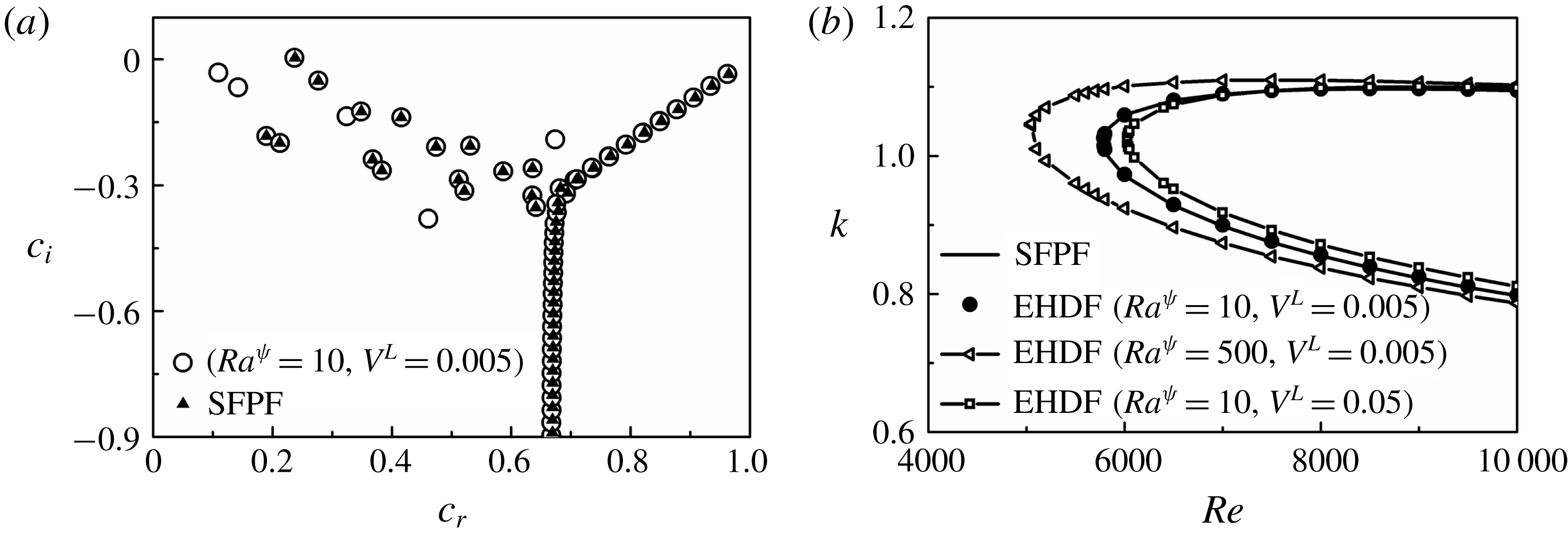
Figure 5. (a) Eigenspectra depicting the real part (
 $c_{r}$
) versus imaginary part (
$c_{r}$
) versus imaginary part (
 $c_{i}$
) of the complex wave speed
$c_{i}$
) of the complex wave speed
 $c$
, for single fluid plane Poiseuille flow (SFPF) and EHD flow (EHDF) when
$c$
, for single fluid plane Poiseuille flow (SFPF) and EHD flow (EHDF) when
 $Re=10\,000$
and
$Re=10\,000$
and
 $k=1$
, and (b) neutral stability curves showing the variation of
$k=1$
, and (b) neutral stability curves showing the variation of
 $k$
with
$k$
with
 $Re$
for SFPF and EHDF. The other parameters considered for EHDF are
$Re$
for SFPF and EHDF. The other parameters considered for EHDF are
 $h=-0.3$
,
$h=-0.3$
,
 $\unicode[STIX]{x1D6FF}=0.02$
and
$\unicode[STIX]{x1D6FF}=0.02$
and
 $Sc=10$
.
$Sc=10$
.
3.4.4 Validation of numerical method
In order to validate the results obtained from the numerical method, we draw a parallel between the EHD flow (abbreviated as EHDF) studied in the present report with the single fluid plane Poiseuille flow (abbreviated as SFPF), as described in Schmid & Henningson (Reference Schmid and Henningson2001) for
 $Re=10\,000$
. The consistency of the numerical method is checked by setting significantly lower values for
$Re=10\,000$
. The consistency of the numerical method is checked by setting significantly lower values for
 $V^{L}$
, representing a negligible viscosity gradient in the flow, so that the flow can be essentially considered to be composed of a single fluid. The electric field force is turned off by assigning extremely low values to
$V^{L}$
, representing a negligible viscosity gradient in the flow, so that the flow can be essentially considered to be composed of a single fluid. The electric field force is turned off by assigning extremely low values to
 $Ra^{\unicode[STIX]{x1D713}}$
. Hence, for imposed constraints of very low
$Ra^{\unicode[STIX]{x1D713}}$
. Hence, for imposed constraints of very low
 $V^{L}$
and
$V^{L}$
and
 $Ra^{\unicode[STIX]{x1D713}}$
, EHDF asymptotically emulates the SFPF. Figure 5 shows the eigenspectra and neutral stability plots for SFPF in tandem with the EHDF considered in the present analysis. Figure 5(a) shows the comparison between the eigenspectra depicting the imaginary part (
$Ra^{\unicode[STIX]{x1D713}}$
, EHDF asymptotically emulates the SFPF. Figure 5 shows the eigenspectra and neutral stability plots for SFPF in tandem with the EHDF considered in the present analysis. Figure 5(a) shows the comparison between the eigenspectra depicting the imaginary part (
 $c_{i}$
) versus the real part (
$c_{i}$
) versus the real part (
 $c_{r}$
) of the complex wave speed,
$c_{r}$
) of the complex wave speed,
 $c$
, for the SFPF and the EHDF. The plot shows that, for a lower electric field potential (
$c$
, for the SFPF and the EHDF. The plot shows that, for a lower electric field potential (
 $Ra^{\unicode[STIX]{x1D713}}=10$
) and marginal viscosity difference (
$Ra^{\unicode[STIX]{x1D713}}=10$
) and marginal viscosity difference (
 $V^{L}=0.005$
), the SFPF and EHDF generate similar eigenspectra. The latter produces a few extra eigenvalues owing to the marginal influence of the electric body force term in the momentum equation. Figure 5(b) depicts the neutral stability curves showing wavenumber (
$V^{L}=0.005$
), the SFPF and EHDF generate similar eigenspectra. The latter produces a few extra eigenvalues owing to the marginal influence of the electric body force term in the momentum equation. Figure 5(b) depicts the neutral stability curves showing wavenumber (
 $k$
) as a function of Reynolds number (
$k$
) as a function of Reynolds number (
 $Re$
) for SFPF and EHDF. For very low values of electric field and viscosity stratification (
$Re$
) for SFPF and EHDF. For very low values of electric field and viscosity stratification (
 $Ra^{\unicode[STIX]{x1D713}}=10$
,
$Ra^{\unicode[STIX]{x1D713}}=10$
,
 $V^{L}=0.005$
), the EHDF shows a similar behaviour to the SFPF, yielding a critical
$V^{L}=0.005$
), the EHDF shows a similar behaviour to the SFPF, yielding a critical
 $Re$
of approximately 5772, as can be seen in figure 5(b). An increase in
$Re$
of approximately 5772, as can be seen in figure 5(b). An increase in
 $Ra^{\unicode[STIX]{x1D713}}$
signals an increment in the destabilizing electric field force, which is reflected as a decreasing trend of the critical
$Ra^{\unicode[STIX]{x1D713}}$
signals an increment in the destabilizing electric field force, which is reflected as a decreasing trend of the critical
 $Re$
with increasing
$Re$
with increasing
 $Ra^{\unicode[STIX]{x1D713}}$
in figure 5(b). However, for a marginal increase in the viscosity difference between the fluids (
$Ra^{\unicode[STIX]{x1D713}}$
in figure 5(b). However, for a marginal increase in the viscosity difference between the fluids (
 $V^{L}=0.05$
) and for a lower electric field potential (
$V^{L}=0.05$
) and for a lower electric field potential (
 $Ra^{\unicode[STIX]{x1D713}}=10$
), the critical
$Ra^{\unicode[STIX]{x1D713}}=10$
), the critical
 $Re$
for instability is found to increase, suggesting a kinetic stabilization of the system. Figure 5 shows the accuracy of the numerical analysis presented in this work, which has been employed to generate the results shown in the manuscript.
$Re$
for instability is found to increase, suggesting a kinetic stabilization of the system. Figure 5 shows the accuracy of the numerical analysis presented in this work, which has been employed to generate the results shown in the manuscript.
3.4.5 Variable ionic mobility
It may be noted here that, the ionic mobility parameter can strongly depend on the viscosity of the fluid (Schmidt & Yoshino Reference Schmidt and Yoshino2015). Thus, it is likely that the ionic mobility values will differ in the fluids of interest in a practical setting. Although in the present analysis, for the purpose of mathematical simplification, most of the results are presented assuming equal ionic mobility, it is however lucrative to study the effect of a difference in the ionic mobility values in order to simulate a physical system with more precision. In order to investigate the effect of ion mobility values on the stability characteristics, we assume the ion mobility to be
 $K_{1}$
in the lower viscosity fluid 1 and
$K_{1}$
in the lower viscosity fluid 1 and
 $K_{2}$
in the higher viscosity fluid 2. The ionic mobility in the mixed interfacial is modelled as
$K_{2}$
in the higher viscosity fluid 2. The ionic mobility in the mixed interfacial is modelled as
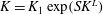 $K=K_{1}\exp (SK^{L})$
, where
$K=K_{1}\exp (SK^{L})$
, where
 $S$
is the same scalar used for defining the viscosity
$S$
is the same scalar used for defining the viscosity
 $\unicode[STIX]{x1D707}$
, and
$\unicode[STIX]{x1D707}$
, and
 $K^{L}=\ln (K_{2}/K_{1})$
, is defined as the log mobility ratio. Subsequently, the perturbation scheme described by (3.19) becomes,
$K^{L}=\ln (K_{2}/K_{1})$
, is defined as the log mobility ratio. Subsequently, the perturbation scheme described by (3.19) becomes,
 $$\begin{eqnarray}\displaystyle [u,w,p,\unicode[STIX]{x1D713},S,\unicode[STIX]{x1D707},K](x,z,t) & = & \displaystyle [u_{0}(z),0,p_{0},\unicode[STIX]{x1D713}_{0}(z),S_{0}(z),\unicode[STIX]{x1D707}_{0}(z),K_{0}(z)]\nonumber\\ \displaystyle & & \displaystyle +\,[\tilde{u} ,\tilde{w},\tilde{p},\tilde{\unicode[STIX]{x1D713}},\tilde{S},\tilde{\unicode[STIX]{x1D707}},\tilde{K}](z)\text{e}^{(\unicode[STIX]{x1D714}t+\text{i}kx)}.\end{eqnarray}$$
The modified governing equation for the conservation of charge density
 $q$
((3.10) and (3.16)) can now be written as,
$q$
((3.10) and (3.16)) can now be written as,
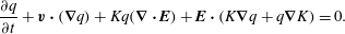 $$\begin{eqnarray}\frac{\unicode[STIX]{x2202}q}{\unicode[STIX]{x2202}t}+\boldsymbol{v}\boldsymbol{\cdot }(\unicode[STIX]{x1D735}q)+Kq(\unicode[STIX]{x1D735}\boldsymbol{\cdot }\boldsymbol{E})+\boldsymbol{E}\boldsymbol{\cdot }(K\unicode[STIX]{x1D735}q+q\unicode[STIX]{x1D735}K)=0.\end{eqnarray}$$
The base-state profile of the ionic mobility
 $K_{0}$
is obtained from the base-state solution of
$K_{0}$
is obtained from the base-state solution of
 $S_{0}$
(3.20) as,
$S_{0}$
(3.20) as,
 $$\begin{eqnarray}K_{0}=\exp (S_{0}K^{L}).\end{eqnarray}$$
The base state of electric potential
 $\unicode[STIX]{x1D713}_{0}$
is obtained by solving the steady-state form of (3.36), given by,
$\unicode[STIX]{x1D713}_{0}$
is obtained by solving the steady-state form of (3.36), given by,
 $$\begin{eqnarray}K_{0}(\unicode[STIX]{x1D713}_{0}^{\prime \prime })^{2}+K_{0}\unicode[STIX]{x1D713}_{0}^{\prime }\unicode[STIX]{x1D713}_{0}^{\prime \prime \prime }+K_{0}^{\prime }\unicode[STIX]{x1D713}_{0}^{\prime }\unicode[STIX]{x1D713}_{0}^{\prime \prime }=0,\end{eqnarray}$$
with the boundary conditions: [
 $\unicode[STIX]{x1D713}_{0}(1)=1;\unicode[STIX]{x1D713}_{0}(-1)=0;\unicode[STIX]{x1D713}_{0}^{\prime \prime }(1)=-I^{q}$
] as already mentioned previously. Upon perturbing the governing equations with the variables mentioned in (3.35), the modified dimensionless linearized charge conservation equation is given by,
$\unicode[STIX]{x1D713}_{0}(1)=1;\unicode[STIX]{x1D713}_{0}(-1)=0;\unicode[STIX]{x1D713}_{0}^{\prime \prime }(1)=-I^{q}$
] as already mentioned previously. Upon perturbing the governing equations with the variables mentioned in (3.35), the modified dimensionless linearized charge conservation equation is given by,
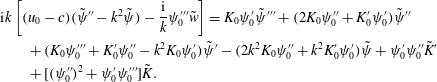 $$\begin{eqnarray}\displaystyle & & \displaystyle \text{i}k\left[(u_{0}-c)(\tilde{\unicode[STIX]{x1D713}}^{\prime \prime }-k^{2}\tilde{\unicode[STIX]{x1D713}})-\frac{\text{i}}{k}\unicode[STIX]{x1D713}_{0}^{\prime \prime \prime }\tilde{w}\right]=K_{0}\unicode[STIX]{x1D713}_{0}^{\prime }\tilde{\unicode[STIX]{x1D713}}^{\prime \prime \prime }+(2K_{0}\unicode[STIX]{x1D713}_{0}^{\prime \prime }+K_{0}^{\prime }\unicode[STIX]{x1D713}_{0}^{\prime })\tilde{\unicode[STIX]{x1D713}}^{\prime \prime }\nonumber\\ \displaystyle & & \displaystyle \qquad +\,(K_{0}\unicode[STIX]{x1D713}_{0}^{\prime \prime \prime }+K_{0}^{\prime }\unicode[STIX]{x1D713}_{0}^{\prime \prime }-k^{2}K_{0}\unicode[STIX]{x1D713}_{0}^{\prime })\tilde{\unicode[STIX]{x1D713}}^{\prime }-(2k^{2}K_{0}\unicode[STIX]{x1D713}_{0}^{\prime \prime }+k^{2}K_{0}^{\prime }\unicode[STIX]{x1D713}_{0}^{\prime })\tilde{\unicode[STIX]{x1D713}}+\unicode[STIX]{x1D713}_{0}^{\prime }\unicode[STIX]{x1D713}_{0}^{\prime \prime }\tilde{K}^{\prime }\nonumber\\ \displaystyle & & \displaystyle \qquad +\,[(\unicode[STIX]{x1D713}_{0}^{\prime \prime })^{2}+\unicode[STIX]{x1D713}_{0}^{\prime }\unicode[STIX]{x1D713}_{0}^{\prime \prime \prime }]\tilde{K}.\end{eqnarray}$$
The linearized non-dimensional governing equations defined by (3.24), (3.39) and (3.26) along with the boundary conditions defined by (3.27)–(3.29), are solved using the numerical method described in § 3.4.3.
3.4.6 Variable dielectric constant
As the case of ionic mobility, it is also quite likely that the experimental fluids seldom have similar dielectric constants. In order to investigate the effect of variable dielectric constants on the stability characteristics, we assume dielectric constants
 $\unicode[STIX]{x1D700}_{1}$
and
$\unicode[STIX]{x1D700}_{1}$
and
 $\unicode[STIX]{x1D700}_{2}$
for fluids 1 and 2, respectively. In the mixed interfacial region, the dielectric constant is modelled as
$\unicode[STIX]{x1D700}_{2}$
for fluids 1 and 2, respectively. In the mixed interfacial region, the dielectric constant is modelled as
 $\unicode[STIX]{x1D700}=\unicode[STIX]{x1D700}_{1}\exp (SE^{L})$
, where
$\unicode[STIX]{x1D700}=\unicode[STIX]{x1D700}_{1}\exp (SE^{L})$
, where
 $E^{L}=\ln (\unicode[STIX]{x1D700}_{2}/\unicode[STIX]{x1D700}_{1})$
is defined as the log permittivity ratio. The perturbation scheme shown in (3.19) transforms into,
$E^{L}=\ln (\unicode[STIX]{x1D700}_{2}/\unicode[STIX]{x1D700}_{1})$
is defined as the log permittivity ratio. The perturbation scheme shown in (3.19) transforms into,
 $$\begin{eqnarray}\displaystyle [u,w,p,\unicode[STIX]{x1D713},S,\unicode[STIX]{x1D707},\unicode[STIX]{x1D700}](x,z,t) & = & \displaystyle [u_{0}(z),0,p_{0},\unicode[STIX]{x1D713}_{0}(z),S_{0}(z),\unicode[STIX]{x1D707}_{0}(z),\unicode[STIX]{x1D700}_{0}(z)]\nonumber\\ \displaystyle & & \displaystyle +\,[\tilde{u} ,\tilde{w},\tilde{p},\tilde{\unicode[STIX]{x1D713}},\tilde{S},\tilde{\unicode[STIX]{x1D707}},\tilde{\unicode[STIX]{x1D700}}](z)\text{e}^{(\unicode[STIX]{x1D714}t+\text{i}kx)}.\end{eqnarray}$$
The base-state profile of dielectric constant
 $\unicode[STIX]{x1D700}_{0}$
is obtained from the base state of the concentration scalar
$\unicode[STIX]{x1D700}_{0}$
is obtained from the base state of the concentration scalar
 $S_{0}$
as,
$S_{0}$
as,
 $$\begin{eqnarray}\unicode[STIX]{x1D700}_{0}=\exp (S_{0}E^{L}).\end{eqnarray}$$
The base-state electric potential
 $\unicode[STIX]{x1D713}_{0}$
is obtained by solving the steady-state form of (3.16), given by,
$\unicode[STIX]{x1D713}_{0}$
is obtained by solving the steady-state form of (3.16), given by,
 $$\begin{eqnarray}\unicode[STIX]{x1D700}_{0}(\unicode[STIX]{x1D713}_{0}^{\prime \prime })^{2}+3\unicode[STIX]{x1D700}_{0}^{\prime }\unicode[STIX]{x1D713}_{0}^{\prime }\unicode[STIX]{x1D713}_{0}^{\prime \prime }+\unicode[STIX]{x1D700}_{0}\unicode[STIX]{x1D713}_{0}^{\prime }\unicode[STIX]{x1D713}_{0}^{\prime \prime \prime }+\unicode[STIX]{x1D700}_{0}^{\prime \prime }(\unicode[STIX]{x1D713}_{0}^{\prime })^{2}=0.\end{eqnarray}$$
Equation (3.42) is solved using the boundary conditions: [
 $\unicode[STIX]{x1D713}_{0}(1)=1;\unicode[STIX]{x1D713}_{0}(-1)=0;\unicode[STIX]{x1D713}_{0}^{\prime \prime }(1)=-I^{q}$
]. The modified dimensionless linearized momentum equation is given by,
$\unicode[STIX]{x1D713}_{0}(1)=1;\unicode[STIX]{x1D713}_{0}(-1)=0;\unicode[STIX]{x1D713}_{0}^{\prime \prime }(1)=-I^{q}$
]. The modified dimensionless linearized momentum equation is given by,
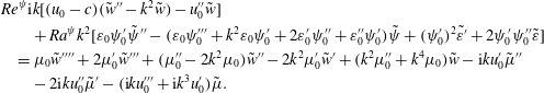 $$\begin{eqnarray}\displaystyle & & \displaystyle Re^{\unicode[STIX]{x1D713}}\text{i}k[(u_{0}-c)(\tilde{w}^{\prime \prime }-k^{2}\tilde{w})-u_{0}^{\prime \prime }\tilde{w}]\nonumber\\ \displaystyle & & \displaystyle \qquad +\,Ra^{\unicode[STIX]{x1D713}}k^{2}[\unicode[STIX]{x1D700}_{0}\unicode[STIX]{x1D713}_{0}^{\prime }\tilde{\unicode[STIX]{x1D713}}^{\prime \prime }-(\unicode[STIX]{x1D700}_{0}\unicode[STIX]{x1D713}_{0}^{\prime \prime \prime }+k^{2}\unicode[STIX]{x1D700}_{0}\unicode[STIX]{x1D713}_{0}^{\prime }+2\unicode[STIX]{x1D700}_{0}^{\prime }\unicode[STIX]{x1D713}_{0}^{\prime \prime }+\unicode[STIX]{x1D700}_{0}^{\prime \prime }\unicode[STIX]{x1D713}_{0}^{\prime })\tilde{\unicode[STIX]{x1D713}}+(\unicode[STIX]{x1D713}_{0}^{\prime })^{2}\tilde{\unicode[STIX]{x1D700}^{\prime }}+2\unicode[STIX]{x1D713}_{0}^{\prime }\unicode[STIX]{x1D713}_{0}^{\prime \prime }\tilde{\unicode[STIX]{x1D700}}]\nonumber\\ \displaystyle & & \displaystyle \quad =\unicode[STIX]{x1D707}_{0}\tilde{w}^{\prime \prime \prime \prime }+2\unicode[STIX]{x1D707}_{0}^{\prime }\tilde{w}^{\prime \prime \prime }+(\unicode[STIX]{x1D707}_{0}^{\prime \prime }-2k^{2}\unicode[STIX]{x1D707}_{0})\tilde{w}^{\prime \prime }-2k^{2}\unicode[STIX]{x1D707}_{0}^{\prime }\tilde{w}^{\prime }+(k^{2}\unicode[STIX]{x1D707}_{0}^{\prime \prime }+k^{4}\unicode[STIX]{x1D707}_{0})\tilde{w}-\text{i}ku_{0}^{\prime }\tilde{\unicode[STIX]{x1D707}}^{\prime \prime }\nonumber\\ \displaystyle & & \displaystyle \qquad -\,2\text{i}ku_{0}^{\prime \prime }\tilde{\unicode[STIX]{x1D707}}^{\prime }-(\text{i}ku_{0}^{\prime \prime \prime }+\text{i}k^{3}u_{0}^{\prime })\tilde{\unicode[STIX]{x1D707}}.\end{eqnarray}$$
The linearized charge conservation equation is given by,
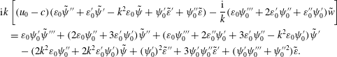 $$\begin{eqnarray}\displaystyle & & \displaystyle \text{i}k\left[(u_{0}-c)(\unicode[STIX]{x1D700}_{0}\tilde{\unicode[STIX]{x1D713}}^{\prime \prime }+\unicode[STIX]{x1D700}_{0}^{\prime }\tilde{\unicode[STIX]{x1D713}^{\prime }}-k^{2}\unicode[STIX]{x1D700}_{0}\tilde{\unicode[STIX]{x1D713}}+\unicode[STIX]{x1D713}_{0}^{\prime }\tilde{\unicode[STIX]{x1D700}}^{\prime }+\unicode[STIX]{x1D713}_{0}^{\prime \prime }\tilde{\unicode[STIX]{x1D700}})-\frac{\text{i}}{k}(\unicode[STIX]{x1D700}_{0}\unicode[STIX]{x1D713}_{0}^{\prime \prime \prime }+2\unicode[STIX]{x1D700}_{0}^{\prime }\unicode[STIX]{x1D713}_{0}^{\prime \prime }+\unicode[STIX]{x1D700}_{0}^{\prime \prime }\unicode[STIX]{x1D713}_{0}^{\prime })\tilde{w}\right]\nonumber\\ \displaystyle & & \displaystyle \quad =\unicode[STIX]{x1D700}_{0}\unicode[STIX]{x1D713}_{0}^{\prime }\tilde{\unicode[STIX]{x1D713}}^{\prime \prime \prime }+(2\unicode[STIX]{x1D700}_{0}\unicode[STIX]{x1D713}_{0}^{\prime \prime }+3\unicode[STIX]{x1D700}_{0}^{\prime }\unicode[STIX]{x1D713}_{0}^{\prime })\tilde{\unicode[STIX]{x1D713}}^{\prime \prime }+(\unicode[STIX]{x1D700}_{0}\unicode[STIX]{x1D713}_{0}^{\prime \prime \prime }+2\unicode[STIX]{x1D700}_{0}^{\prime \prime }\unicode[STIX]{x1D713}_{0}^{\prime }+3\unicode[STIX]{x1D700}_{0}^{\prime }\unicode[STIX]{x1D713}_{0}^{\prime \prime }-k^{2}\unicode[STIX]{x1D700}_{0}\unicode[STIX]{x1D713}_{0}^{\prime })\tilde{\unicode[STIX]{x1D713}}^{\prime }\nonumber\\ \displaystyle & & \displaystyle \qquad -\,(2k^{2}\unicode[STIX]{x1D700}_{0}\unicode[STIX]{x1D713}_{0}^{\prime \prime }+2k^{2}\unicode[STIX]{x1D700}_{0}^{\prime }\unicode[STIX]{x1D713}_{0}^{\prime })\tilde{\unicode[STIX]{x1D713}}+(\unicode[STIX]{x1D713}_{0}^{\prime })^{2}\tilde{\unicode[STIX]{x1D700}}^{\prime \prime }+3\unicode[STIX]{x1D713}_{0}^{\prime }\unicode[STIX]{x1D713}_{0}^{\prime \prime }\tilde{\unicode[STIX]{x1D700}}^{\prime }+(\unicode[STIX]{x1D713}_{0}^{\prime }\unicode[STIX]{x1D713}_{0}^{\prime \prime \prime }+\unicode[STIX]{x1D713}_{0}^{\prime \prime 2})\tilde{\unicode[STIX]{x1D700}}.\end{eqnarray}$$
Equations (3.43) and (3.44) along with (3.26) are solved using the boundary conditions mentioned in (3.27)–(3.29) applying the numerical method discussed in § 3.4.3.
3.5 Nonlinear simulations
The computational domain for the nonlinear simulations is shown in figure 3(b). The properties of the fluids are modelled as,
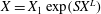 $X=X_{1}\exp (SX^{L})$
, where
$X=X_{1}\exp (SX^{L})$
, where
 $X$
is a physical property (viscosity (
$X$
is a physical property (viscosity (
 $\unicode[STIX]{x1D707}_{1}$
,
$\unicode[STIX]{x1D707}_{1}$
,
 $\unicode[STIX]{x1D707}_{2}$
), dielectric constant (
$\unicode[STIX]{x1D707}_{2}$
), dielectric constant (
 $\unicode[STIX]{x1D700}_{1}$
,
$\unicode[STIX]{x1D700}_{1}$
,
 $\unicode[STIX]{x1D700}_{2}$
) or ionic mobility (
$\unicode[STIX]{x1D700}_{2}$
) or ionic mobility (
 $K_{1}$
,
$K_{1}$
,
 $K_{2}$
)),
$K_{2}$
)),
 $S$
is any scalar and
$S$
is any scalar and
 $X^{L}$
is the log ratio. The governing equations simulated for the system are same as defined in § 3.2 ((3.2)–(3.11)).
$X^{L}$
is the log ratio. The governing equations simulated for the system are same as defined in § 3.2 ((3.2)–(3.11)).
For the flow field ((3.2) and (3.3)), a no-slip (
 $\boldsymbol{v}=0$
) condition was enforced at the walls. For the advection–diffusion equation (3.11), the inlet concentration was fixed at 1 for the higher viscosity (dielectric constant, ionic mobility) fluid and at 0 for the lower one. For the electric field (3.6),
$\boldsymbol{v}=0$
) condition was enforced at the walls. For the advection–diffusion equation (3.11), the inlet concentration was fixed at 1 for the higher viscosity (dielectric constant, ionic mobility) fluid and at 0 for the lower one. For the electric field (3.6),
 $\unicode[STIX]{x1D713}=\unicode[STIX]{x1D6F9}_{0}$
and
$\unicode[STIX]{x1D713}=\unicode[STIX]{x1D6F9}_{0}$
and
 $\unicode[STIX]{x1D713}=0$
boundary conditions were enforced at the top and bottom electrodes, respectively. The injection was considered autonomous and homogenous (refer to § 2.2). Thus, for the charge conservation equation defined by (3.7), constant charge density,
$\unicode[STIX]{x1D713}=0$
boundary conditions were enforced at the top and bottom electrodes, respectively. The injection was considered autonomous and homogenous (refer to § 2.2). Thus, for the charge conservation equation defined by (3.7), constant charge density,
 $q=Q_{0}$
, was maintained at the injector (top). It was also assumed that the ions discharged immediately on reaching the collector electrode (Wu et al.
Reference Wu, Traoré, Vázquez and Pérez2013, Reference Wu, Pérez, Traoré and Vázquez2015).
$q=Q_{0}$
, was maintained at the injector (top). It was also assumed that the ions discharged immediately on reaching the collector electrode (Wu et al.
Reference Wu, Traoré, Vázquez and Pérez2013, Reference Wu, Pérez, Traoré and Vázquez2015).
The set of partial differential equations defined by (3.2)–(3.11) were solved using the finite element method employing the commercial software COMSOL Multiphysics™ for a 2-D geometry shown in figure 3(b). The domain was discretized with
 ${\sim}4.5\times 10^{4}$
finite elements with refinement along the walls, mixed interface and electrode regions. Second-order elements for velocity, concentration, potential and volume charge density, and first-order elements for pressure, were used for discretization. The MUltifrontal Massively Parallel Sparse direct solver (MUMPS) was used for solving the equations. The time dependent solver was adjusted to a backward difference formula with free time stepping for integrating the equations.
${\sim}4.5\times 10^{4}$
finite elements with refinement along the walls, mixed interface and electrode regions. Second-order elements for velocity, concentration, potential and volume charge density, and first-order elements for pressure, were used for discretization. The MUltifrontal Massively Parallel Sparse direct solver (MUMPS) was used for solving the equations. The time dependent solver was adjusted to a backward difference formula with free time stepping for integrating the equations.
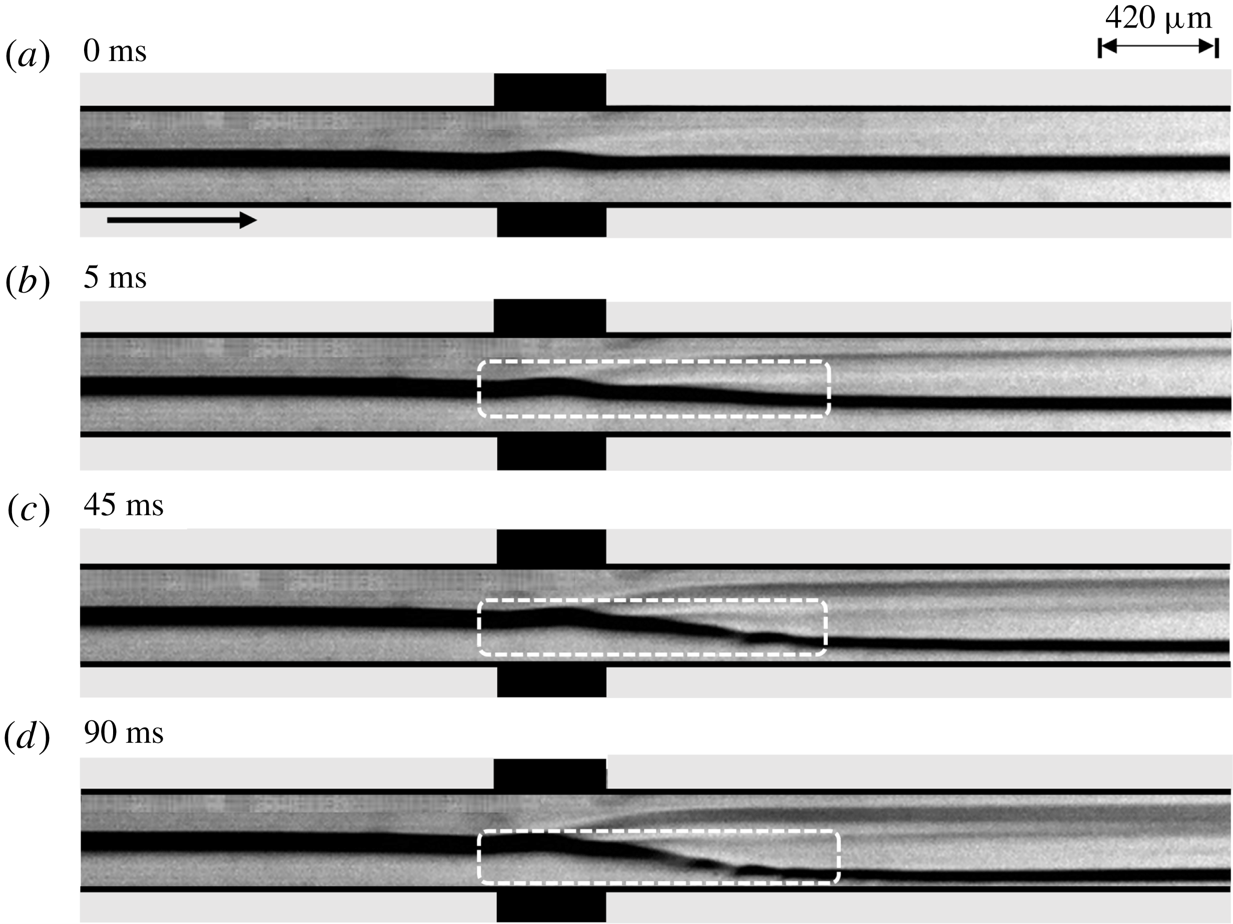
Figure 6. (a–d) Show the experimental snapshots after 0 ms, 5 ms, 45 ms and 90 ms, respectively, depicting the response of a stratified flow of a benzene–silicone oil system through the microchannel under an applied potential of 300 V (
 $Ra^{\unicode[STIX]{x1D713}}=225$
). Here, (a) corresponds to the system under 0 V electric potential. The top layer on the image corresponds to benzene and the bottom layer corresponds to silicone oil. The fluids flowed side by side in the channel while the images were taken from the top. The average
$Ra^{\unicode[STIX]{x1D713}}=225$
). Here, (a) corresponds to the system under 0 V electric potential. The top layer on the image corresponds to benzene and the bottom layer corresponds to silicone oil. The fluids flowed side by side in the channel while the images were taken from the top. The average
 $Re$
of the base flow was maintained approximately at 0.5. The arrow indicates the direction of flow.
$Re$
of the base flow was maintained approximately at 0.5. The arrow indicates the direction of flow.
4 Results and discussion
4.1 Experimental observations
We initiate the discussion with one of the experimental results in which a benzene–silicone oil system (
 $V^{L}\approx 6$
) flowed through a microchannel before the EHD field was generated by the application of a DC voltage of 300 V (
$V^{L}\approx 6$
) flowed through a microchannel before the EHD field was generated by the application of a DC voltage of 300 V (
 $Ra^{\unicode[STIX]{x1D713}}=225$
) across the electrodes. Figure 6 shows the images of the experiment, which correspond to the top view of the flow while the electrodes were inserted into the channel horizontally from the sides, as previously mentioned in figure 1. The supporting movie 1 available at https://doi.org/10.1017/jfm.2018.1023 shows the spatio-temporal evolution of the instability near the electrode with the finer details. The experiments were visualized using a microscope under 2.5
$Ra^{\unicode[STIX]{x1D713}}=225$
) across the electrodes. Figure 6 shows the images of the experiment, which correspond to the top view of the flow while the electrodes were inserted into the channel horizontally from the sides, as previously mentioned in figure 1. The supporting movie 1 available at https://doi.org/10.1017/jfm.2018.1023 shows the spatio-temporal evolution of the instability near the electrode with the finer details. The experiments were visualized using a microscope under 2.5
 $\times$
magnification and recorded using a high speed camera at 500 fps at a resolution of
$\times$
magnification and recorded using a high speed camera at 500 fps at a resolution of
 $1280\times 120$
pixels unless stated otherwise. It may be noted here that a higher difference in the viscosities of benzene and silicone oil helped us in capturing the high quality grey scale videos, as reported here. The EHD instability phenomenon was reproducible for benzene–oleic acid and benzene–soybean oil systems too. However, those results are not reported for the sake of brevity. Figure 6(a) shows that the pressure-driven flow rates of the fluids were attuned in such a manner that a steady stratified flow was formed in the absence of the external field. Figure 6(b–d) and the supporting movie 1 show the typical evolution of the miscible benzene–silicone oil interface under the influence of the electric field. It may be noted here that the top layer shown in the image is benzene while the bottom one is silicone oil. However, in reality, the fluids flowed side by side in the channel while the images were taken from the top. On application of the electric field potential through the electrodes, the flow becomes unstable and develops instabilities, as shown with the help of highlighted rectangular boxes in the images. The images and the video suggest that the applied field destabilizes the lower viscosity benzene layer and subsequently shifts the diffused interface towards the more viscous silicone oil layer. Under the exposure of a constant electric field intensity, the instability possesses convective waves propagating towards the downstream of the channel owing to the presence of the pressure-driven flow inside the channel. After the onset, the speed of these waves increase with time before reaching a constant value for given field intensity, as shown in figure 6(b–d) and the supporting movie 1.
$1280\times 120$
pixels unless stated otherwise. It may be noted here that a higher difference in the viscosities of benzene and silicone oil helped us in capturing the high quality grey scale videos, as reported here. The EHD instability phenomenon was reproducible for benzene–oleic acid and benzene–soybean oil systems too. However, those results are not reported for the sake of brevity. Figure 6(a) shows that the pressure-driven flow rates of the fluids were attuned in such a manner that a steady stratified flow was formed in the absence of the external field. Figure 6(b–d) and the supporting movie 1 show the typical evolution of the miscible benzene–silicone oil interface under the influence of the electric field. It may be noted here that the top layer shown in the image is benzene while the bottom one is silicone oil. However, in reality, the fluids flowed side by side in the channel while the images were taken from the top. On application of the electric field potential through the electrodes, the flow becomes unstable and develops instabilities, as shown with the help of highlighted rectangular boxes in the images. The images and the video suggest that the applied field destabilizes the lower viscosity benzene layer and subsequently shifts the diffused interface towards the more viscous silicone oil layer. Under the exposure of a constant electric field intensity, the instability possesses convective waves propagating towards the downstream of the channel owing to the presence of the pressure-driven flow inside the channel. After the onset, the speed of these waves increase with time before reaching a constant value for given field intensity, as shown in figure 6(b–d) and the supporting movie 1.
4.2 Theoretical outlook of the instabilities
The details of the theoretical formulation are deliberated in § 3 while the results obtained from the LSA are discussed in this section. We have identified that, for the proposed system, the effects of
 $Ra^{\unicode[STIX]{x1D713}}$
,
$Ra^{\unicode[STIX]{x1D713}}$
,
 $V^{L}$
and
$V^{L}$
and
 $Sc$
are perhaps the most significant ones because all of the different modes of instability pertaining to this system are obtained with variations in the magnitudes of these parameters. The results (except for figures 13–15) correspond to
$Sc$
are perhaps the most significant ones because all of the different modes of instability pertaining to this system are obtained with variations in the magnitudes of these parameters. The results (except for figures 13–15) correspond to
 $K_{L}=0$
and
$K_{L}=0$
and
 $E_{L}=0$
, unless otherwise stated. Figure 7(a) depicts the neutral stability plot showing the variation of the wavenumber (
$E_{L}=0$
, unless otherwise stated. Figure 7(a) depicts the neutral stability plot showing the variation of the wavenumber (
 $k$
) with
$k$
) with
 $Ra^{\unicode[STIX]{x1D713}}$
for
$Ra^{\unicode[STIX]{x1D713}}$
for
 $V^{L}=1$
. The plot suggests that the system is unstable to a finite-wavenumber mode of instability at low and intermediate values of
$V^{L}=1$
. The plot suggests that the system is unstable to a finite-wavenumber mode of instability at low and intermediate values of
 $Ra^{\unicode[STIX]{x1D713}}$
(solid line). We term this mode the electric field mode I (E-I). At higher values of
$Ra^{\unicode[STIX]{x1D713}}$
(solid line). We term this mode the electric field mode I (E-I). At higher values of
 $Ra^{\unicode[STIX]{x1D713}}$
the system becomes unstable to another finite-wavenumber mode of instability (broken line) termed the electric field mode II (E-II). The wave speed (
$Ra^{\unicode[STIX]{x1D713}}$
the system becomes unstable to another finite-wavenumber mode of instability (broken line) termed the electric field mode II (E-II). The wave speed (
 $c_{r}$
) of the E-I-mode is found to match with the theoretical average velocity (
$c_{r}$
) of the E-I-mode is found to match with the theoretical average velocity (
 $u_{0}$
) of the lower viscosity fluid (fluid 1) whereas the wave speed of the E-II-mode matches with the mean flow of the higher viscosity fluid (fluid 2). This observation helps in inferring that the EHD field can destabilize the lower viscosity fluid at much lower values of
$u_{0}$
) of the lower viscosity fluid (fluid 1) whereas the wave speed of the E-II-mode matches with the mean flow of the higher viscosity fluid (fluid 2). This observation helps in inferring that the EHD field can destabilize the lower viscosity fluid at much lower values of
 $Ra^{\unicode[STIX]{x1D713}}$
to manifest the E-I-mode while the E-II-mode appears at a much higher value of
$Ra^{\unicode[STIX]{x1D713}}$
to manifest the E-I-mode while the E-II-mode appears at a much higher value of
 $Ra^{\unicode[STIX]{x1D713}}$
in the higher viscosity fluid 2. The typical
$Ra^{\unicode[STIX]{x1D713}}$
in the higher viscosity fluid 2. The typical
 $\unicode[STIX]{x1D714}$
versus
$\unicode[STIX]{x1D714}$
versus
 $k$
plots with the variation in
$k$
plots with the variation in
 $Ra^{\unicode[STIX]{x1D713}}$
are shown in figure 7(d). At
$Ra^{\unicode[STIX]{x1D713}}$
are shown in figure 7(d). At
 $Ra^{\unicode[STIX]{x1D713}}=400$
, only E-I-mode exists (unevenly broken line) whereas at
$Ra^{\unicode[STIX]{x1D713}}=400$
, only E-I-mode exists (unevenly broken line) whereas at
 $Ra^{\unicode[STIX]{x1D713}}=1125$
, both E-I and E-II modes (triangular symbols) are present with the E-I-mode characterized by significantly higher growth rates than the E-II-mode. Figure 7(b) illustrates the variation of wavenumber against log viscosity ratio (
$Ra^{\unicode[STIX]{x1D713}}=1125$
, both E-I and E-II modes (triangular symbols) are present with the E-I-mode characterized by significantly higher growth rates than the E-II-mode. Figure 7(b) illustrates the variation of wavenumber against log viscosity ratio (
 $V^{L}$
) for
$V^{L}$
) for
 $Ra^{\unicode[STIX]{x1D713}}=375$
. The plot suggests that, at lower values of
$Ra^{\unicode[STIX]{x1D713}}=375$
. The plot suggests that, at lower values of
 $V^{L}$
, only the E-I-mode (solid line) can destabilize the flow. In comparison, at higher values of
$V^{L}$
, only the E-I-mode (solid line) can destabilize the flow. In comparison, at higher values of
 $V^{L}$
, a much longer-wavelength viscous mode (V) (unevenly broken line) appears alongside the E-I-mode. At the intermediate values of
$V^{L}$
, a much longer-wavelength viscous mode (V) (unevenly broken line) appears alongside the E-I-mode. At the intermediate values of
 $V^{L}$
, ranging from 1.3 to 1.6, a unique bimodal behaviour is observed, as shown by the
$V^{L}$
, ranging from 1.3 to 1.6, a unique bimodal behaviour is observed, as shown by the
 $\unicode[STIX]{x1D714}$
versus
$\unicode[STIX]{x1D714}$
versus
 $k$
plots in figure 7(e). The plots clearly suggest that the V-mode arises only when there is a higher viscosity contrast across the diffused interface. Figure 7(c) shows the variation of
$k$
plots in figure 7(e). The plots clearly suggest that the V-mode arises only when there is a higher viscosity contrast across the diffused interface. Figure 7(c) shows the variation of
 $k$
with
$k$
with
 $Sc$
for
$Sc$
for
 $V^{L}=2$
and
$V^{L}=2$
and
 $Ra^{\unicode[STIX]{x1D713}}=375$
. In this situation, apart from the E-I mode (solid line), the diffusive D-mode becomes unstable beyond a threshold value of
$Ra^{\unicode[STIX]{x1D713}}=375$
. In this situation, apart from the E-I mode (solid line), the diffusive D-mode becomes unstable beyond a threshold value of
 $Sc$
. The D-mode exhibits a finite-wavenumber-type behaviour for low to intermediate values of
$Sc$
. The D-mode exhibits a finite-wavenumber-type behaviour for low to intermediate values of
 $Sc$
, which signifies a thick and diffusive interface. At higher values of
$Sc$
, which signifies a thick and diffusive interface. At higher values of
 $Sc$
, when the interface is much sharper and thinner, the D-mode behaves as a long-wave mode, frequently observed for immiscible two-phase flows (Ern et al.
Reference Ern, Charru and Luchini2003; Sahu & Govindarajan Reference Sahu and Govindarajan2016). The
$Sc$
, when the interface is much sharper and thinner, the D-mode behaves as a long-wave mode, frequently observed for immiscible two-phase flows (Ern et al.
Reference Ern, Charru and Luchini2003; Sahu & Govindarajan Reference Sahu and Govindarajan2016). The
 $\unicode[STIX]{x1D714}$
versus
$\unicode[STIX]{x1D714}$
versus
 $k$
plots in figure 7(f) shows the transition of the length scale from the shorter- to longer-wavelength regime with the increase in
$k$
plots in figure 7(f) shows the transition of the length scale from the shorter- to longer-wavelength regime with the increase in
 $Sc$
.
$Sc$
.

Figure 7. Neutral stability plots showing the variations of wavenumber (
 $k$
) with (a) electric Rayleigh number
$k$
) with (a) electric Rayleigh number
 $Ra^{\unicode[STIX]{x1D713}}$
, (b) log viscosity ratio
$Ra^{\unicode[STIX]{x1D713}}$
, (b) log viscosity ratio
 $V^{L}$
and (c) Schmidt number
$V^{L}$
and (c) Schmidt number
 $Sc$
. The dispersion curves showing the growth rate (
$Sc$
. The dispersion curves showing the growth rate (
 $\unicode[STIX]{x1D714}$
) versus the wavenumber (
$\unicode[STIX]{x1D714}$
) versus the wavenumber (
 $k$
) of the unstable modes with (d)
$k$
) of the unstable modes with (d)
 $Ra^{\unicode[STIX]{x1D713}}$
, (e)
$Ra^{\unicode[STIX]{x1D713}}$
, (e)
 $V^{L}$
and (f)
$V^{L}$
and (f)
 $Sc$
. In (a) the solid line represents the electric field mode I (E-I) and the broken line represents the electric field mode II (E-II). The other parameters for (a,d) are
$Sc$
. In (a) the solid line represents the electric field mode I (E-I) and the broken line represents the electric field mode II (E-II). The other parameters for (a,d) are
 $V^{L}=1$
,
$V^{L}=1$
,
 $h=-0.3$
,
$h=-0.3$
,
 $\unicode[STIX]{x1D6FF}=0.02$
,
$\unicode[STIX]{x1D6FF}=0.02$
,
 $Sc=10$
and
$Sc=10$
and
 $Re=0.5$
. In (b) the solid lines represent electric field mode I (E-I) and the unevenly broken lines represent the viscous mode (V). The other parameters for (b,e) are
$Re=0.5$
. In (b) the solid lines represent electric field mode I (E-I) and the unevenly broken lines represent the viscous mode (V). The other parameters for (b,e) are
 $h=-0.3$
,
$h=-0.3$
,
 $\unicode[STIX]{x1D6FF}=0.02$
,
$\unicode[STIX]{x1D6FF}=0.02$
,
 $Sc=10$
,
$Sc=10$
,
 $Ra^{\unicode[STIX]{x1D713}}=375$
and
$Ra^{\unicode[STIX]{x1D713}}=375$
and
 $Re=0.5$
. In (c) the solid lines represent the E-I-mode, the unevenly broken line represents the V-mode and the evenly broken line denotes the diffusive mode (D). The other parameters for (c,f) are
$Re=0.5$
. In (c) the solid lines represent the E-I-mode, the unevenly broken line represents the V-mode and the evenly broken line denotes the diffusive mode (D). The other parameters for (c,f) are
 $V^{L}=2$
,
$V^{L}=2$
,
 $h=-0.3$
,
$h=-0.3$
,
 $\unicode[STIX]{x1D6FF}=0.02$
,
$\unicode[STIX]{x1D6FF}=0.02$
,
 $Ra^{\unicode[STIX]{x1D713}}=375$
and
$Ra^{\unicode[STIX]{x1D713}}=375$
and
 $Re=0.5$
. The hatched U-regions denote unstable zones whereas S-regions denote the stable zones.
$Re=0.5$
. The hatched U-regions denote unstable zones whereas S-regions denote the stable zones.
Figure 8. The variations of (a) normalized energy (
 $E_{N}$
) with
$E_{N}$
) with
 $Ra^{\unicode[STIX]{x1D713}}$
, (b) normalized energy with
$Ra^{\unicode[STIX]{x1D713}}$
, (b) normalized energy with
 $V^{L}$
, (c) absolute values of normalized perturbation concentration (
$V^{L}$
, (c) absolute values of normalized perturbation concentration (
 $\tilde{S}$
) with
$\tilde{S}$
) with
 $Sc$
and (d) normalized energy with
$Sc$
and (d) normalized energy with
 $Sc$
. The other parameters for (a) are
$Sc$
. The other parameters for (a) are
 $V^{L}=1$
,
$V^{L}=1$
,
 $h=-0.7$
,
$h=-0.7$
,
 $\unicode[STIX]{x1D6FF}=0.02$
,
$\unicode[STIX]{x1D6FF}=0.02$
,
 $Sc=10$
and
$Sc=10$
and
 $Re=0.5$
. The other parameters for (b) are
$Re=0.5$
. The other parameters for (b) are
 $h=-0.3$
,
$h=-0.3$
,
 $\unicode[STIX]{x1D6FF}=0.02$
,
$\unicode[STIX]{x1D6FF}=0.02$
,
 $Sc=10$
,
$Sc=10$
,
 $Ra^{\unicode[STIX]{x1D713}}=375$
and
$Ra^{\unicode[STIX]{x1D713}}=375$
and
 $Re=0.5$
. The other parameters for (c,d) are
$Re=0.5$
. The other parameters for (c,d) are
 $V^{L}=3$
,
$V^{L}=3$
,
 $h=-0.3$
,
$h=-0.3$
,
 $\unicode[STIX]{x1D6FF}=0.02$
,
$\unicode[STIX]{x1D6FF}=0.02$
,
 $Ra^{\unicode[STIX]{x1D713}}=375$
and
$Ra^{\unicode[STIX]{x1D713}}=375$
and
 $Re=0.5$
.
$Re=0.5$
.
In summary, figure 7 uncovers four distinctive finite-wavenumber modes destabilizing a two-layer viscosity stratified flow of miscible fluids under the influence of an externally applied electric field. The results suggest the existence of two distinct electric field modes, E-I and E-II, beyond a critical value of
 $Ra^{\unicode[STIX]{x1D713}}$
. Further, the presence of the V- and D-modes are also observed due to the viscosity stratification and convective transport of the perturbed concentration near the interface, respectively.
$Ra^{\unicode[STIX]{x1D713}}$
. Further, the presence of the V- and D-modes are also observed due to the viscosity stratification and convective transport of the perturbed concentration near the interface, respectively.
In order to evaluate the contributions of the various forces to the growth of the instability modes discussed above, an energy analysis is carried out. A brief outline of the analysis is provided in appendix A. The energy equation relates the rate of change of the disturbance kinetic energy (
 $E_{KE}$
), with energy changes associated with the Reynolds stress (
$E_{KE}$
), with energy changes associated with the Reynolds stress (
 $E_{RS}$
), viscous dissipation (
$E_{RS}$
), viscous dissipation (
 $E_{VD}$
), viscosity stratification (
$E_{VD}$
), viscosity stratification (
 $E_{V}$
) and electric force (
$E_{V}$
) and electric force (
 $E_{E}$
) components. Figure 8 describes the variation of the normalized energy associated with the various terms (
$E_{E}$
) components. Figure 8 describes the variation of the normalized energy associated with the various terms (
 $E_{N}$
) with
$E_{N}$
) with
 $Ra^{\unicode[STIX]{x1D713}}$
,
$Ra^{\unicode[STIX]{x1D713}}$
,
 $V^{L}$
and
$V^{L}$
and
 $Sc$
. It may be noted here that the eigenfunctions used for the energy calculations correspond to those of the most unstable modes. Further, the eigenfunctions are normalized with their maximum absolute values while the energy terms are normalized by the total kinetic energy
$Sc$
. It may be noted here that the eigenfunctions used for the energy calculations correspond to those of the most unstable modes. Further, the eigenfunctions are normalized with their maximum absolute values while the energy terms are normalized by the total kinetic energy
 $\int _{-1}^{1}(|\tilde{u} |^{2}+|\tilde{w}|^{2})\,\text{d}z$
. The variation of
$\int _{-1}^{1}(|\tilde{u} |^{2}+|\tilde{w}|^{2})\,\text{d}z$
. The variation of
 $E_{RS}$
is not shown in the plots because the energy associated with the Reynolds stresses are negligible for the flows with low
$E_{RS}$
is not shown in the plots because the energy associated with the Reynolds stresses are negligible for the flows with low
 $Re$
reported in this work.
$Re$
reported in this work.
Figure 8(a) shows that, for the situation with a lower viscosity stratification (
 $V^{L}=1$
), the major part of the disturbance energy is generated by the applied electric force, which is reflected in the higher values of
$V^{L}=1$
), the major part of the disturbance energy is generated by the applied electric force, which is reflected in the higher values of
 $E_{E}$
. With the increase in electric force (
$E_{E}$
. With the increase in electric force (
 $Ra^{\unicode[STIX]{x1D713}}$
),
$Ra^{\unicode[STIX]{x1D713}}$
),
 $E_{E}$
increases monotonically, which is the cause of the onset of the E-I and E-II modes. In this case, the energy associated with viscosity stratification (
$E_{E}$
increases monotonically, which is the cause of the onset of the E-I and E-II modes. In this case, the energy associated with viscosity stratification (
 $E_{V}$
) is negligible, and remains nearly unchanged with increment in
$E_{V}$
) is negligible, and remains nearly unchanged with increment in
 $Ra^{\unicode[STIX]{x1D713}}$
. The trends of the variation in
$Ra^{\unicode[STIX]{x1D713}}$
. The trends of the variation in
 $E_{E}$
and
$E_{E}$
and
 $E_{V}$
with
$E_{V}$
with
 $Ra^{\unicode[STIX]{x1D713}}$
explain well the occurrence of the electric field modes at lower viscosity stratifications, as previously discussed with figure 7(a,d). Figure 8(b) depicts the variations of
$Ra^{\unicode[STIX]{x1D713}}$
explain well the occurrence of the electric field modes at lower viscosity stratifications, as previously discussed with figure 7(a,d). Figure 8(b) depicts the variations of
 $E_{N}$
with
$E_{N}$
with
 $V^{L}$
, which reveals that the electric force remains the major source of disturbance at lower values of
$V^{L}$
, which reveals that the electric force remains the major source of disturbance at lower values of
 $V^{L}$
. Hence, for lower viscosity stratifications, only the E-I-mode of instability manifests in the system, as depicted in figure 7(b,e). With the increase in
$V^{L}$
. Hence, for lower viscosity stratifications, only the E-I-mode of instability manifests in the system, as depicted in figure 7(b,e). With the increase in
 $V^{L}$
, the energy associated with viscosity stratification increases rapidly, leading to the occurrence of the V-mode of instability along with the E-I-mode. Figure 8(c) shows the variation of the absolute values of the normalized perturbation concentration (
$V^{L}$
, the energy associated with viscosity stratification increases rapidly, leading to the occurrence of the V-mode of instability along with the E-I-mode. Figure 8(c) shows the variation of the absolute values of the normalized perturbation concentration (
 $\tilde{S}$
) for different values of
$\tilde{S}$
) for different values of
 $Sc$
. At lower values of
$Sc$
. At lower values of
 $Sc$
the variation in
$Sc$
the variation in
 $\tilde{S}$
is found to be progressive and less steep near the mixed interface. The variation in
$\tilde{S}$
is found to be progressive and less steep near the mixed interface. The variation in
 $\tilde{S}$
becomes steeper across the interface at higher values of
$\tilde{S}$
becomes steeper across the interface at higher values of
 $Sc$
, which gives rise to the onset of the D-mode of instability. Figure 8(d) shows the variation of
$Sc$
, which gives rise to the onset of the D-mode of instability. Figure 8(d) shows the variation of
 $E_{N}$
with
$E_{N}$
with
 $Sc$
. The plot suggests that at lower values of
$Sc$
. The plot suggests that at lower values of
 $Sc$
, the disturbance kinetic energy is produced mainly by the applied electric force, which is indicated by the higher values of
$Sc$
, the disturbance kinetic energy is produced mainly by the applied electric force, which is indicated by the higher values of
 $E_{E}$
. At higher values of
$E_{E}$
. At higher values of
 $Sc$
,
$Sc$
,
 $E_{V}$
contributes more towards the generation of disturbance energy compared to
$E_{V}$
contributes more towards the generation of disturbance energy compared to
 $E_{E}$
, which causes the D-mode to occur alongside the E-I-mode, as previously observed in figure 7(c,f).
$E_{E}$
, which causes the D-mode to occur alongside the E-I-mode, as previously observed in figure 7(c,f).

Figure 9. Neutral stability plots showing the variation of wavenumber (
 $k$
) versus electric field Rayleigh number (
$k$
) versus electric field Rayleigh number (
 $Ra^{\unicode[STIX]{x1D713}}$
) for (a)
$Ra^{\unicode[STIX]{x1D713}}$
) for (a)
 $V^{L}=0$
, (b)
$V^{L}=0$
, (b)
 $V^{L}=1$
, (c)
$V^{L}=1$
, (c)
 $V^{L}=2$
and (d)
$V^{L}=2$
and (d)
 $V^{L}=3$
. In (b–d) the evenly broken, solid, dotted and unevenly broken lines show the situations with
$V^{L}=3$
. In (b–d) the evenly broken, solid, dotted and unevenly broken lines show the situations with
 $h=-0.9,-0.3,0$
and 0.35, respectively. The other parameters are
$h=-0.9,-0.3,0$
and 0.35, respectively. The other parameters are
 $Sc=10$
,
$Sc=10$
,
 $\unicode[STIX]{x1D6FF}=0.02$
and
$\unicode[STIX]{x1D6FF}=0.02$
and
 $Re=0.5$
. The hatched U-regions denote unstable zones whereas S-regions denote the stable zones.
$Re=0.5$
. The hatched U-regions denote unstable zones whereas S-regions denote the stable zones.

Figure 10. (a) Shows the variations of dominant growth rate (
 $\unicode[STIX]{x1D714}_{m}$
, denoted by symbols) and wavelength (
$\unicode[STIX]{x1D714}_{m}$
, denoted by symbols) and wavelength (
 $\unicode[STIX]{x1D706}_{m}$
, denoted by lines) with
$\unicode[STIX]{x1D706}_{m}$
, denoted by lines) with
 $Ra^{\unicode[STIX]{x1D713}}$
. (b,c) Show the variations of dominant growth rate (
$Ra^{\unicode[STIX]{x1D713}}$
. (b,c) Show the variations of dominant growth rate (
 $\unicode[STIX]{x1D714}_{m}$
, denoted by symbols) and wavelength (
$\unicode[STIX]{x1D714}_{m}$
, denoted by symbols) and wavelength (
 $\unicode[STIX]{x1D706}_{m}$
, denoted by lines) with
$\unicode[STIX]{x1D706}_{m}$
, denoted by lines) with
 $h$
, at different values of
$h$
, at different values of
 $Ra^{\unicode[STIX]{x1D713}}$
for
$Ra^{\unicode[STIX]{x1D713}}$
for
 $V^{L}=1$
and
$V^{L}=1$
and
 $V^{L}=2$
, respectively. The other parameters considered for (a) are
$V^{L}=2$
, respectively. The other parameters considered for (a) are
 $V^{L}=1$
,
$V^{L}=1$
,
 $h=-0.3$
,
$h=-0.3$
,
 $\unicode[STIX]{x1D6FF}=0.02$
,
$\unicode[STIX]{x1D6FF}=0.02$
,
 $Sc=10$
and
$Sc=10$
and
 $Re=0.5$
. The other parameters considered for (b,c) are
$Re=0.5$
. The other parameters considered for (b,c) are
 $h=-0.3$
,
$h=-0.3$
,
 $\unicode[STIX]{x1D6FF}=0.02$
,
$\unicode[STIX]{x1D6FF}=0.02$
,
 $Sc=10$
and
$Sc=10$
and
 $Re=0.5$
.
$Re=0.5$
.
4.2.1 Parametric study
In this section we discuss the role of various parameters in influencing the stability of the system. Figure 9(b) shows the variation of
 $k$
with
$k$
with
 $Ra^{\unicode[STIX]{x1D713}}$
for different values of
$Ra^{\unicode[STIX]{x1D713}}$
for different values of
 $h$
, which signifies the distance of the diffused interface from the datum,
$h$
, which signifies the distance of the diffused interface from the datum,
 $z=0$
, as previously shown in figure 3(a). It may be noted here that the variation of
$z=0$
, as previously shown in figure 3(a). It may be noted here that the variation of
 $h$
from
$h$
from
 $-$
1 to 1 also signifies the progressive filling of the channel with a more viscous fluid. Figure 9(a) shows the situation when
$-$
1 to 1 also signifies the progressive filling of the channel with a more viscous fluid. Figure 9(a) shows the situation when
 $V^{L}$
 $=$
0, which indicates that the channel is entirely filled with the low viscosity fluid. The plot shows that the system is unstable to the E-I-mode of instability. In figure 9(b–d) the evenly broken, solid, dotted and unevenly broken lines show the situations with
$=$
0, which indicates that the channel is entirely filled with the low viscosity fluid. The plot shows that the system is unstable to the E-I-mode of instability. In figure 9(b–d) the evenly broken, solid, dotted and unevenly broken lines show the situations with
 $h=-0.9$
,
$h=-0.9$
,
 $-0.3$
, 0 and 0.35, respectively, which signify that the channel is filled with thin (e.g.
$-0.3$
, 0 and 0.35, respectively, which signify that the channel is filled with thin (e.g.
 $h=-0.9$
) to thick (e.g.
$h=-0.9$
) to thick (e.g.
 $h=0.35$
) layers of more viscous fluid in the fully developed stratified flow.
$h=0.35$
) layers of more viscous fluid in the fully developed stratified flow.
Figure 9(b) shows the neutral stability curves when
 $V^{L}=1$
, for different values of
$V^{L}=1$
, for different values of
 $h$
. The plot suggests that as the proportion of the more viscous fluid increases inside the channel, the critical
$h$
. The plot suggests that as the proportion of the more viscous fluid increases inside the channel, the critical
 $Ra^{\unicode[STIX]{x1D713}}$
for the E-I-mode progressively increases owing to the increase in the overall viscous resistance. The neutral stability curves in figure 9(c) for
$Ra^{\unicode[STIX]{x1D713}}$
for the E-I-mode progressively increases owing to the increase in the overall viscous resistance. The neutral stability curves in figure 9(c) for
 $V^{L}=2$
show the presence of the E-I-mode for the situations with a thinner layer of more viscous fluid. The plot shows the appearance of the twin E-I and V modes with shorter and longer wavelengths, respectively, as the thickness of the layer with more viscosity is increased at
$V^{L}=2$
show the presence of the E-I-mode for the situations with a thinner layer of more viscous fluid. The plot shows the appearance of the twin E-I and V modes with shorter and longer wavelengths, respectively, as the thickness of the layer with more viscosity is increased at
 $h=-0.3$
. The V-mode arises due to the viscosity stratification across the diffused interface, while the origin of the E-I-mode can be attributed to the externally applied electric field, as discussed previously. Notably, the E-I-mode is found to have a much shorter wavelength, compared to the V-mode. The V-mode becomes unstable at a much lower value of
$h=-0.3$
. The V-mode arises due to the viscosity stratification across the diffused interface, while the origin of the E-I-mode can be attributed to the externally applied electric field, as discussed previously. Notably, the E-I-mode is found to have a much shorter wavelength, compared to the V-mode. The V-mode becomes unstable at a much lower value of
 $Ra^{\unicode[STIX]{x1D713}}$
when the thickness of the more and less viscous fluids are identical at
$Ra^{\unicode[STIX]{x1D713}}$
when the thickness of the more and less viscous fluids are identical at
 $h=0$
. With further increase in the thickness of the higher viscosity fluid, the increase in the viscous resistance inside the channel enforces the V-mode to appear at a higher value of
$h=0$
. With further increase in the thickness of the higher viscosity fluid, the increase in the viscous resistance inside the channel enforces the V-mode to appear at a higher value of
 $Ra^{\unicode[STIX]{x1D713}}$
for
$Ra^{\unicode[STIX]{x1D713}}$
for
 $h=0.35$
. Again, the E-I-mode for this plot appears at a much higher value of
$h=0.35$
. Again, the E-I-mode for this plot appears at a much higher value of
 $Ra^{\unicode[STIX]{x1D713}}$
, which is not shown. Figure 9(d) shows the results for
$Ra^{\unicode[STIX]{x1D713}}$
, which is not shown. Figure 9(d) shows the results for
 $V^{L}=3$
, which are very similar in nature to those observed in figure 9(c). However, for
$V^{L}=3$
, which are very similar in nature to those observed in figure 9(c). However, for
 $V^{L}=3$
, the V-mode becomes unstable even in the absence of an externally applied electric field beyond a certain value of
$V^{L}=3$
, the V-mode becomes unstable even in the absence of an externally applied electric field beyond a certain value of
 $h$
, as can be seen for
$h$
, as can be seen for
 $h=0$
and
$h=0$
and
 $h=0.35$
. Thus, the V-mode is found to have similar characteristics to the shear mode of instability in the viscosity stratified flow of miscible fluids, which has been reported in previous works (Talon & Meiburg Reference Talon and Meiburg2011).
$h=0.35$
. Thus, the V-mode is found to have similar characteristics to the shear mode of instability in the viscosity stratified flow of miscible fluids, which has been reported in previous works (Talon & Meiburg Reference Talon and Meiburg2011).
Figure 11. (a) Shows the variations of dominant growth rate (
 $\unicode[STIX]{x1D714}_{m}$
, denoted by symbols), and wavelength (
$\unicode[STIX]{x1D714}_{m}$
, denoted by symbols), and wavelength (
 $\unicode[STIX]{x1D706}_{m}$
, denoted by lines) with
$\unicode[STIX]{x1D706}_{m}$
, denoted by lines) with
 $V^{L}$
. The other parameters considered are
$V^{L}$
. The other parameters considered are
 $h=-0.3$
,
$h=-0.3$
,
 $\unicode[STIX]{x1D6FF}=0.02$
,
$\unicode[STIX]{x1D6FF}=0.02$
,
 $Sc=10$
,
$Sc=10$
,
 $Ra^{\unicode[STIX]{x1D713}}=375$
and
$Ra^{\unicode[STIX]{x1D713}}=375$
and
 $Re=0.5$
. (b) Shows the variations of dominant growth rate (
$Re=0.5$
. (b) Shows the variations of dominant growth rate (
 $\unicode[STIX]{x1D714}_{m}$
, denoted by symbols) and wavelength (
$\unicode[STIX]{x1D714}_{m}$
, denoted by symbols) and wavelength (
 $\unicode[STIX]{x1D706}_{m}$
, denoted by lines) with
$\unicode[STIX]{x1D706}_{m}$
, denoted by lines) with
 $h$
for different values of
$h$
for different values of
 $Sc$
. The other parameters are,
$Sc$
. The other parameters are,
 $V^{L}=2$
,
$V^{L}=2$
,
 $\unicode[STIX]{x1D6FF}=0.02$
,
$\unicode[STIX]{x1D6FF}=0.02$
,
 $Ra^{\unicode[STIX]{x1D713}}=375$
and
$Ra^{\unicode[STIX]{x1D713}}=375$
and
 $Re=0.5$
.
$Re=0.5$
.
Figure 10(a) depicts the variations of the dominant growth rate (
 $\unicode[STIX]{x1D714}_{m}$
) and wavelength (
$\unicode[STIX]{x1D714}_{m}$
) and wavelength (
 $\unicode[STIX]{x1D706}_{m}$
) representing the most unstable disturbances with
$\unicode[STIX]{x1D706}_{m}$
) representing the most unstable disturbances with
 $Ra^{\unicode[STIX]{x1D713}}$
for
$Ra^{\unicode[STIX]{x1D713}}$
for
 $V^{L}=1$
. The plot suggests that, for low and intermediate values of
$V^{L}=1$
. The plot suggests that, for low and intermediate values of
 $Ra^{\unicode[STIX]{x1D713}}$
, the system manifests the E-I-mode (black symbols) whereas at higher values of field intensity the E-II-mode (red symbols) appears along with the E-I-mode. Figure 10(b) shows the variations of
$Ra^{\unicode[STIX]{x1D713}}$
, the system manifests the E-I-mode (black symbols) whereas at higher values of field intensity the E-II-mode (red symbols) appears along with the E-I-mode. Figure 10(b) shows the variations of
 $\unicode[STIX]{x1D714}_{m}$
and
$\unicode[STIX]{x1D714}_{m}$
and
 $\unicode[STIX]{x1D706}_{m}$
with
$\unicode[STIX]{x1D706}_{m}$
with
 $h$
across the channel for three different values of
$h$
across the channel for three different values of
 $Ra^{\unicode[STIX]{x1D713}}$
. Again, in this plot the variation of
$Ra^{\unicode[STIX]{x1D713}}$
. Again, in this plot the variation of
 $h$
from
$h$
from
 $-1$
to 1 signifies the progressive filling of the channel with the more viscous fluid. The plot suggests that when
$-1$
to 1 signifies the progressive filling of the channel with the more viscous fluid. The plot suggests that when
 $V^{L}=1$
, the E-I-mode progressively loses its strength (
$V^{L}=1$
, the E-I-mode progressively loses its strength (
 $\unicode[STIX]{x1D714}_{m}$
reduces) when the channel is filled with the more viscous fluid provided
$\unicode[STIX]{x1D714}_{m}$
reduces) when the channel is filled with the more viscous fluid provided
 $Ra^{\unicode[STIX]{x1D713}}$
is kept constant. Subsequently, a marginal increase in
$Ra^{\unicode[STIX]{x1D713}}$
is kept constant. Subsequently, a marginal increase in
 $\unicode[STIX]{x1D706}_{m}$
of the E-I-mode is also observed. The plot also shows that the time and length scales of the E-I-mode reduce with the increase in
$\unicode[STIX]{x1D706}_{m}$
of the E-I-mode is also observed. The plot also shows that the time and length scales of the E-I-mode reduce with the increase in
 $Ra^{\unicode[STIX]{x1D713}}$
because the magnitude of
$Ra^{\unicode[STIX]{x1D713}}$
because the magnitude of
 $\unicode[STIX]{x1D714}_{m}$
increases and
$\unicode[STIX]{x1D714}_{m}$
increases and
 $\unicode[STIX]{x1D706}_{m}$
reduces with the increase in
$\unicode[STIX]{x1D706}_{m}$
reduces with the increase in
 $Ra^{\unicode[STIX]{x1D713}}$
. In comparison, figure 10(c) shows that, for higher values of
$Ra^{\unicode[STIX]{x1D713}}$
. In comparison, figure 10(c) shows that, for higher values of
 $V^{L}$
(
$V^{L}$
(
 $V^{L}=2$
), the E-I-mode is the dominant one at lower values of
$V^{L}=2$
), the E-I-mode is the dominant one at lower values of
 $h$
. However, the reduction in
$h$
. However, the reduction in
 $\unicode[STIX]{x1D714}_{m}$
of the E-I-mode happens at a much faster rate with the increase in
$\unicode[STIX]{x1D714}_{m}$
of the E-I-mode happens at a much faster rate with the increase in
 $h$
while a subdominant V-mode appears due to the combined influence of electric field and viscosity stratification at intermediate values of
$h$
while a subdominant V-mode appears due to the combined influence of electric field and viscosity stratification at intermediate values of
 $h$
. At even higher values of
$h$
. At even higher values of
 $h$
, the E-I-mode disappears, and the V-mode becomes the dominant mode. Interestingly, at intermediate values of
$h$
, the E-I-mode disappears, and the V-mode becomes the dominant mode. Interestingly, at intermediate values of
 $h$
both the modes co-exist to engender a bimodal instability. The plot suggests that the time and length scales of both the E-I-mode and V-mode reduce with the increase in
$h$
both the modes co-exist to engender a bimodal instability. The plot suggests that the time and length scales of both the E-I-mode and V-mode reduce with the increase in
 $Ra^{\unicode[STIX]{x1D713}}$
because the magnitude of
$Ra^{\unicode[STIX]{x1D713}}$
because the magnitude of
 $\unicode[STIX]{x1D714}_{m}$
increases and
$\unicode[STIX]{x1D714}_{m}$
increases and
 $\unicode[STIX]{x1D706}_{m}$
reduces with the increase in
$\unicode[STIX]{x1D706}_{m}$
reduces with the increase in
 $Ra^{\unicode[STIX]{x1D713}}$
as previously observed in the case of
$Ra^{\unicode[STIX]{x1D713}}$
as previously observed in the case of
 $V^{L}=1$
. Thus, an externally applied electric field can stimulate both the finite-wavenumber E-I and V modes at lower
$V^{L}=1$
. Thus, an externally applied electric field can stimulate both the finite-wavenumber E-I and V modes at lower
 $Re$
of the stratified flow of miscible fluids.
$Re$
of the stratified flow of miscible fluids.
Another important parameter, which strongly influences the nature of the instabilities in the present setting, is the viscosity contrast between the fluids defined by log viscosity ratio
 $V^{L}$
. Figure 11(a) shows the variations of
$V^{L}$
. Figure 11(a) shows the variations of
 $\unicode[STIX]{x1D714}_{m}$
and
$\unicode[STIX]{x1D714}_{m}$
and
 $\unicode[STIX]{x1D706}_{m}$
with
$\unicode[STIX]{x1D706}_{m}$
with
 $V^{L}$
. The plot suggests that when the viscosity contrast across the diffused interface is lower, the E-I-mode is the dominant one whereas, with a progressive increase in
$V^{L}$
. The plot suggests that when the viscosity contrast across the diffused interface is lower, the E-I-mode is the dominant one whereas, with a progressive increase in
 $V^{L}$
, the V-mode can become the dominant one (not shown here). The plot also shows a much smaller length scale of the E-I-mode as compared to the V-mode. It is important to note here that
$V^{L}$
, the V-mode can become the dominant one (not shown here). The plot also shows a much smaller length scale of the E-I-mode as compared to the V-mode. It is important to note here that
 $Sc$
is another crucial parameter for defining the stability of miscible flows. The effect of
$Sc$
is another crucial parameter for defining the stability of miscible flows. The effect of
 $Sc$
on various configurations of miscible flows have been discussed in detail in previous literature (Sahu & Govindarajan Reference Sahu and Govindarajan2016). However, the presence of an electric field in this regard makes the study more interesting. It has been discussed earlier that the
$Sc$
on various configurations of miscible flows have been discussed in detail in previous literature (Sahu & Govindarajan Reference Sahu and Govindarajan2016). However, the presence of an electric field in this regard makes the study more interesting. It has been discussed earlier that the
 $Sc$
number contributes to the appearance of the D-mode beyond a critical threshold. Figure 11(b) shows the variation of
$Sc$
number contributes to the appearance of the D-mode beyond a critical threshold. Figure 11(b) shows the variation of
 $\unicode[STIX]{x1D714}_{m}$
and
$\unicode[STIX]{x1D714}_{m}$
and
 $\unicode[STIX]{x1D706}_{m}$
with
$\unicode[STIX]{x1D706}_{m}$
with
 $h$
for three different values of
$h$
for three different values of
 $Sc$
. It can be inferred from the figure that the E-I-mode remains almost unaffected by the increase in
$Sc$
. It can be inferred from the figure that the E-I-mode remains almost unaffected by the increase in
 $Sc$
. However, as the interface becomes thinner and less diffusive (higher
$Sc$
. However, as the interface becomes thinner and less diffusive (higher
 $Sc$
, filled circular and triangular symbols) the V-mode which occurs at
$Sc$
, filled circular and triangular symbols) the V-mode which occurs at
 $Sc=10$
undergoes transition to the D-mode which is accompanied by a drastic increase in the growth rates of the most unstable perturbations. At higher values of
$Sc=10$
undergoes transition to the D-mode which is accompanied by a drastic increase in the growth rates of the most unstable perturbations. At higher values of
 $h$
, again the increase in the viscous resistance owing to the presence of the more viscous liquid reduces the growth rate of the D-mode.
$h$
, again the increase in the viscous resistance owing to the presence of the more viscous liquid reduces the growth rate of the D-mode.
It is now well understood that the thickness of the mixed interface plays a significant role in determining the stability characteristics of the system (Talon & Meiburg Reference Talon and Meiburg2011). While a thicker mixed interface damps a perturbation due to molecular diffusion, a thin interface with restricted diffusion makes a perturbation unstable owing to steep viscosity profiles near the interfacial region. The neutral stability plot shown in figure 12(a) describes the effect of
 $\unicode[STIX]{x1D6FF}$
on the stability behaviour for
$\unicode[STIX]{x1D6FF}$
on the stability behaviour for
 $V^{L}=2$
. While the E-I-mode remains unaffected by
$V^{L}=2$
. While the E-I-mode remains unaffected by
 $\unicode[STIX]{x1D6FF}$
, the V-mode exhibits profound stabilization with an increase in
$\unicode[STIX]{x1D6FF}$
, the V-mode exhibits profound stabilization with an increase in
 $\unicode[STIX]{x1D6FF}$
. Apart from the interfacial thickness, the level of charge injection,
$\unicode[STIX]{x1D6FF}$
. Apart from the interfacial thickness, the level of charge injection,
 $I^{q}$
, can also influence the critical conditions of the E-I-mode. Figure 12(b) shows that the critical
$I^{q}$
, can also influence the critical conditions of the E-I-mode. Figure 12(b) shows that the critical
 $Ra^{\unicode[STIX]{x1D713}}$
reduces significantly with the increase in
$Ra^{\unicode[STIX]{x1D713}}$
reduces significantly with the increase in
 $I^{q}$
. This observation is in qualitative agreement with the results of Zhang et al. (Reference Zhang, Martinelli, Wu, Schmid and Quadrio2015) for a single fluid.
$I^{q}$
. This observation is in qualitative agreement with the results of Zhang et al. (Reference Zhang, Martinelli, Wu, Schmid and Quadrio2015) for a single fluid.
Figure 12. Neutral stability plots showing the variation of
 $k$
with
$k$
with
 $Ra^{\unicode[STIX]{x1D713}}$
for (a) different values of thickness of the mixed interface,
$Ra^{\unicode[STIX]{x1D713}}$
for (a) different values of thickness of the mixed interface,
 $\unicode[STIX]{x1D6FF}$
, and (b) different values of the injection level
$\unicode[STIX]{x1D6FF}$
, and (b) different values of the injection level
 $I^{q}$
. The other parameters for (a) are
$I^{q}$
. The other parameters for (a) are
 $V^{L}=2$
,
$V^{L}=2$
,
 $h=-0.3$
,
$h=-0.3$
,
 $Sc=10$
and
$Sc=10$
and
 $Re=0.5$
and for (b) are
$Re=0.5$
and for (b) are
 $V^{L}=1$
,
$V^{L}=1$
,
 $h=-0.3$
,
$h=-0.3$
,
 $\unicode[STIX]{x1D6FF}=0.02$
,
$\unicode[STIX]{x1D6FF}=0.02$
,
 $Sc=10$
and
$Sc=10$
and
 $Re=0.5$
. The hatched U-regions denote unstable zones whereas S-regions denote the stable zones.
$Re=0.5$
. The hatched U-regions denote unstable zones whereas S-regions denote the stable zones.
The difference in ionic mobility in the two fluids can be a critical parameter in governing the stability characteristics of the system under study. The base-state profile for electric potential
 $\unicode[STIX]{x1D713}_{0}$
is shown in figure 13 for different values of
$\unicode[STIX]{x1D713}_{0}$
is shown in figure 13 for different values of
 $K^{L}$
. The variation of ionic mobility across the channel is consequential in the distribution electric potential across the channel. In the case of uniform mobility across the channel (
$K^{L}$
. The variation of ionic mobility across the channel is consequential in the distribution electric potential across the channel. In the case of uniform mobility across the channel (
 $K^{L}=0$
), the base-state profile of electric potential is progressive, as shown in figure 13. However, with a decrease in the value of ionic mobility in the higher viscosity fluid, there is a build-up of charge in the mixed interfacial region, which is depicted by the cusps in the profiles of the electric potential
$K^{L}=0$
), the base-state profile of electric potential is progressive, as shown in figure 13. However, with a decrease in the value of ionic mobility in the higher viscosity fluid, there is a build-up of charge in the mixed interfacial region, which is depicted by the cusps in the profiles of the electric potential
 $\unicode[STIX]{x1D713}_{0}$
near the mixed interfacial region for
$\unicode[STIX]{x1D713}_{0}$
near the mixed interfacial region for
 $K^{L}=-2$
,
$K^{L}=-2$
,
 $K^{L}=-3$
and
$K^{L}=-3$
and
 $K^{L}=-4$
. Figure 14(a) depicts the neutral stability plots for different values of
$K^{L}=-4$
. Figure 14(a) depicts the neutral stability plots for different values of
 $K^{L}$
, at
$K^{L}$
, at
 $V^{L}=1$
and
$V^{L}=1$
and
 $h=-0.7$
. It can be inferred from the plot that, as the mobility values decrease in the higher viscosity fluid, the critical electric field needed to trigger the E-I-mode of instability increases. However, with an increase in the proportion of the more viscous fluid (
$h=-0.7$
. It can be inferred from the plot that, as the mobility values decrease in the higher viscosity fluid, the critical electric field needed to trigger the E-I-mode of instability increases. However, with an increase in the proportion of the more viscous fluid (
 $h=-0.3$
), there is a substantial increase in the growth rates (
$h=-0.3$
), there is a substantial increase in the growth rates (
 $\unicode[STIX]{x1D714}_{m}$
) at
$\unicode[STIX]{x1D714}_{m}$
) at
 $K^{L}=-3$
and
$K^{L}=-3$
and
 $K^{L}=-4$
, compared to
$K^{L}=-4$
, compared to
 $K^{L}=0$
as seen from figure 14(b,c). The instabilities also exhibit much shorter wavelengths compared to the finite-wavenumber E-I-mode of instability. We hereafter refer to this mode as the K-mode of instability. Figure 14(d) shows the variation of
$K^{L}=0$
as seen from figure 14(b,c). The instabilities also exhibit much shorter wavelengths compared to the finite-wavenumber E-I-mode of instability. We hereafter refer to this mode as the K-mode of instability. Figure 14(d) shows the variation of
 $\unicode[STIX]{x1D714}_{m}$
with the location of the mixed layer (h). It can be inferred from the plot that, for greater proportions of less viscous (higher mobility) fluid inside the channel, the system becomes unstable to the E-I-mode of instability (triangular symbols). The interface is located close to the walls when the proportion of either fluid is very high inside the channel. Thus, any perturbation occurring within the interfacial region due to difference in ionic mobility is stabilized by viscous dissipation. Thus, only the E-I-mode occurs for high proportions of the less viscous fluid inside the channel. With an increase in the proportion of the more viscous (lesser mobility) fluid, as the location of the interface
$\unicode[STIX]{x1D714}_{m}$
with the location of the mixed layer (h). It can be inferred from the plot that, for greater proportions of less viscous (higher mobility) fluid inside the channel, the system becomes unstable to the E-I-mode of instability (triangular symbols). The interface is located close to the walls when the proportion of either fluid is very high inside the channel. Thus, any perturbation occurring within the interfacial region due to difference in ionic mobility is stabilized by viscous dissipation. Thus, only the E-I-mode occurs for high proportions of the less viscous fluid inside the channel. With an increase in the proportion of the more viscous (lesser mobility) fluid, as the location of the interface
 $h$
shifts towards the centre of the channel, the instability is governed by the K-mode with higher growth rates and lower wavelength as compared to the E-I-mode. The K-mode occurs in the mixed interfacial region due the steep gradient in charge density in the region caused by the difference in ionic mobility between the fluids. Again, it can be seen from figure 14(e,f) that, for higher viscosity stratification, the stability characteristics change on varying the ionic mobility of the fluids. For
$h$
shifts towards the centre of the channel, the instability is governed by the K-mode with higher growth rates and lower wavelength as compared to the E-I-mode. The K-mode occurs in the mixed interfacial region due the steep gradient in charge density in the region caused by the difference in ionic mobility between the fluids. Again, it can be seen from figure 14(e,f) that, for higher viscosity stratification, the stability characteristics change on varying the ionic mobility of the fluids. For
 $K^{L}=-4$
, as depicted by figure 14(f), only the K-mode of instability exists, unlike the V-mode and the E-I-mode depicted in figure 14(e) for
$K^{L}=-4$
, as depicted by figure 14(f), only the K-mode of instability exists, unlike the V-mode and the E-I-mode depicted in figure 14(e) for
 $K^{L}=0$
. It may be noted that with a further increase in viscosity stratification, the V-mode also occurs in conjunction with the K-mode (not shown here).
$K^{L}=0$
. It may be noted that with a further increase in viscosity stratification, the V-mode also occurs in conjunction with the K-mode (not shown here).
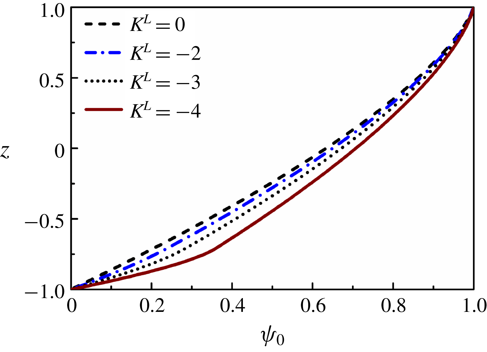
Figure 13. Base-state profile for electric potential (
 $\unicode[STIX]{x1D713}_{0}$
) for different values of log mobility ratio
$\unicode[STIX]{x1D713}_{0}$
) for different values of log mobility ratio
 $K^{L}$
. The other parameters are
$K^{L}$
. The other parameters are
 $h=-0.3$
and
$h=-0.3$
and
 $\unicode[STIX]{x1D6FF}=0.02$
.
$\unicode[STIX]{x1D6FF}=0.02$
.
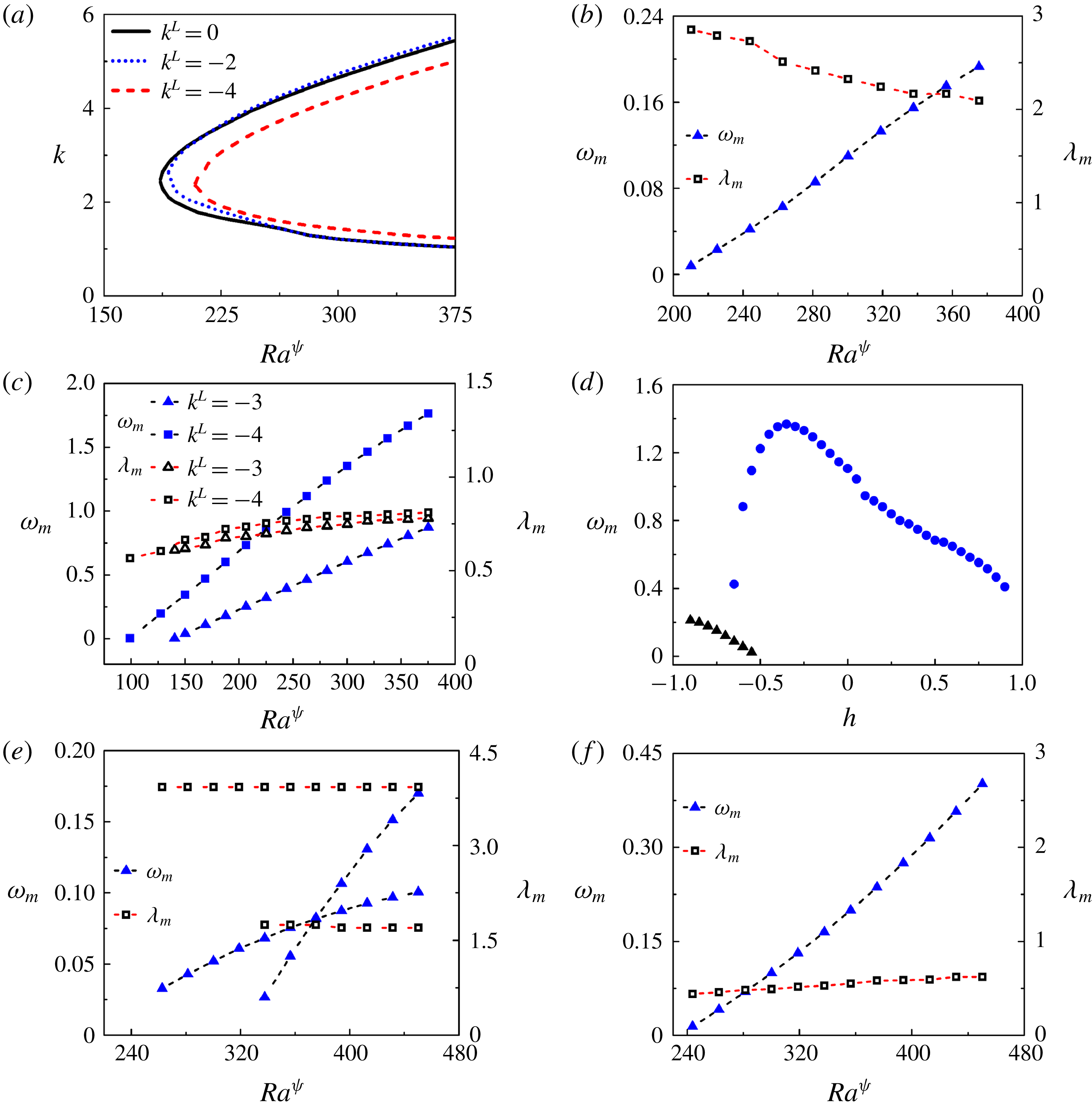
Figure 14. (a) Neutral stability curves showing the variation of wavenumber (
 $k$
) with electric Rayleigh number (
$k$
) with electric Rayleigh number (
 $Ra^{\unicode[STIX]{x1D713}}$
) for different values of
$Ra^{\unicode[STIX]{x1D713}}$
) for different values of
 $K^{L}$
. The other parameters are
$K^{L}$
. The other parameters are
 $V^{L}=1$
,
$V^{L}=1$
,
 $h=-0.7$
,
$h=-0.7$
,
 $\unicode[STIX]{x1D6FF}=0.02$
,
$\unicode[STIX]{x1D6FF}=0.02$
,
 $Sc=10$
and
$Sc=10$
and
 $Re=0.5$
. Variation of the growth rate of the most unstable modes (
$Re=0.5$
. Variation of the growth rate of the most unstable modes (
 $\unicode[STIX]{x1D714}_{m}$
) with
$\unicode[STIX]{x1D714}_{m}$
) with
 $Ra^{\unicode[STIX]{x1D713}}$
for (b)
$Ra^{\unicode[STIX]{x1D713}}$
for (b)
 $K^{L}=0$
, (c)
$K^{L}=0$
, (c)
 $K^{L}=-3$
and
$K^{L}=-3$
and
 $K^{L}=-4$
. The other parameters used for (b,c) are
$K^{L}=-4$
. The other parameters used for (b,c) are
 $V^{L}=1$
,
$V^{L}=1$
,
 $h=-0.3$
,
$h=-0.3$
,
 $\unicode[STIX]{x1D6FF}=0.02$
,
$\unicode[STIX]{x1D6FF}=0.02$
,
 $Sc=10$
and
$Sc=10$
and
 $Re=0.5$
. (d) Variation of the growth rate of the most unstable modes (
$Re=0.5$
. (d) Variation of the growth rate of the most unstable modes (
 $\unicode[STIX]{x1D714}_{m}$
) for different values of
$\unicode[STIX]{x1D714}_{m}$
) for different values of
 $h$
. The other parameters used are
$h$
. The other parameters used are
 $V^{L}=1$
,
$V^{L}=1$
,
 $K^{L}=-4$
,
$K^{L}=-4$
,
 $Ra^{\unicode[STIX]{x1D713}}=300$
,
$Ra^{\unicode[STIX]{x1D713}}=300$
,
 $\unicode[STIX]{x1D6FF}=0.02$
,
$\unicode[STIX]{x1D6FF}=0.02$
,
 $Sc=10$
and
$Sc=10$
and
 $Re=0.5$
. Variation of the growth rate of the most unstable modes (
$Re=0.5$
. Variation of the growth rate of the most unstable modes (
 $\unicode[STIX]{x1D714}_{m}$
) with
$\unicode[STIX]{x1D714}_{m}$
) with
 $Ra^{\unicode[STIX]{x1D713}}$
for
$Ra^{\unicode[STIX]{x1D713}}$
for
 $V^{L}=2$
and (e)
$V^{L}=2$
and (e)
 $K^{L}=0$
and (f)
$K^{L}=0$
and (f)
 $K^{L}=-4$
. The other parameters are
$K^{L}=-4$
. The other parameters are
 $h=-0.3$
,
$h=-0.3$
,
 $\unicode[STIX]{x1D6FF}=0.02$
,
$\unicode[STIX]{x1D6FF}=0.02$
,
 $Sc=10$
and
$Sc=10$
and
 $Re=0.5$
.
$Re=0.5$
.
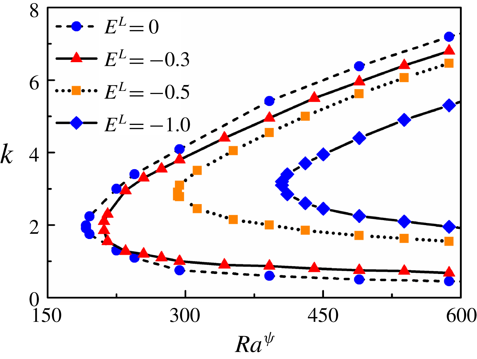
Figure 15. Neutral stability curves showing the variation of wavenumber (
 $k$
) with electric Rayleigh number (
$k$
) with electric Rayleigh number (
 $Ra^{\unicode[STIX]{x1D713}}$
) for different values of
$Ra^{\unicode[STIX]{x1D713}}$
) for different values of
 $E^{L}$
. The other parameters are
$E^{L}$
. The other parameters are
 $V^{L}=1$
,
$V^{L}=1$
,
 $K^{L}=0$
,
$K^{L}=0$
,
 $h=-0.3$
,
$h=-0.3$
,
 $\unicode[STIX]{x1D6FF}=0.02$
,
$\unicode[STIX]{x1D6FF}=0.02$
,
 $Sc=10$
and
$Sc=10$
and
 $Re=0.5$
.
$Re=0.5$
.
The dielectric constant is another important parameter that can be consequential to the stability characteristics of the system under study. Figure 15 shows the neutral stability curves depicting the variation of
 $k$
with
$k$
with
 $Ra^{\unicode[STIX]{x1D713}}$
for different values of
$Ra^{\unicode[STIX]{x1D713}}$
for different values of
 $E^{L}$
. The plot predicts an increase in the critical values of
$E^{L}$
. The plot predicts an increase in the critical values of
 $Ra^{\unicode[STIX]{x1D713}}$
with an increase in the permittivity stratification inside the channel compared to the case of uniform permittivity (
$Ra^{\unicode[STIX]{x1D713}}$
with an increase in the permittivity stratification inside the channel compared to the case of uniform permittivity (
 $E^{L}=0$
). It may be noted here that, in this work, the higher permittivity is used as the characteristic permittivity. Hence, negative (positive) sign in the value of
$E^{L}=0$
). It may be noted here that, in this work, the higher permittivity is used as the characteristic permittivity. Hence, negative (positive) sign in the value of
 $E^{L}$
signifies that the permittivity of fluid 2 is lesser (higher) than that of fluid 1. It can be inferred from figure 15 that, for slight differences in the values of electric permittivity of the two fluids, the critical conditions for the onset of the instabilities remain very close to each other. Significant changes in the onset conditions are only observed for larger differences in the values of dielectric constants of the two fluids. Since this study is motivated by fluids with similar dielectric constants, we do not undertake an in-depth analysis of the consequences of larger contrasts in the dielectric constants.
$E^{L}$
signifies that the permittivity of fluid 2 is lesser (higher) than that of fluid 1. It can be inferred from figure 15 that, for slight differences in the values of electric permittivity of the two fluids, the critical conditions for the onset of the instabilities remain very close to each other. Significant changes in the onset conditions are only observed for larger differences in the values of dielectric constants of the two fluids. Since this study is motivated by fluids with similar dielectric constants, we do not undertake an in-depth analysis of the consequences of larger contrasts in the dielectric constants.
Figures 7–15 together provide some clue to the onset of instability in a two-layer viscosity stratified flow of miscible fluids, which has been observed in the experiment shown in figure 6. The plots reveal that the E-I-mode may appear even at very low flow rates beyond a critical electric field intensity, which suggests that the proposed methodology can cause micromixing in the low
 $Re$
flows. The threshold field intensity to instigate the instability can be reduced further by increasing the charge injection level, reducing the diffusion across the interface, and reducing the proportion of more viscous fluid. Further, both the layers can be made unstable at higher field intensities by simultaneously stimulating both the E-I and E-II modes. Conditionally, the V-mode and D-modes may appear owing to the viscosity contrast across the interface and the convective transport at the diffused interface. A contrast in the ionic mobilities in the two fluids may also cause the appearance of the K-mode of instability characterized by higher growth rates compared to the E-I-mode. For small values of
$Re$
flows. The threshold field intensity to instigate the instability can be reduced further by increasing the charge injection level, reducing the diffusion across the interface, and reducing the proportion of more viscous fluid. Further, both the layers can be made unstable at higher field intensities by simultaneously stimulating both the E-I and E-II modes. Conditionally, the V-mode and D-modes may appear owing to the viscosity contrast across the interface and the convective transport at the diffused interface. A contrast in the ionic mobilities in the two fluids may also cause the appearance of the K-mode of instability characterized by higher growth rates compared to the E-I-mode. For small values of
 $E^{L}$
, the nature and onset conditions of the instabilities are similar to the case of uniform dielectric constants.
$E^{L}$
, the nature and onset conditions of the instabilities are similar to the case of uniform dielectric constants.
4.3 A comparison between experimental and theoretical results
In this section, a comparison between the data obtained from the experiments, LSA and numerical simulations is reported. Here, we particularly focus on the critical voltage required to initiate the instability in the two-layer stratified flow of miscible fluids. Due to limitations in measurement techniques, the values of
 $h$
and
$h$
and
 $\unicode[STIX]{x1D6FF}$
used for the theoretical calculations are assumed to emulate the experimental conditions closely. The precise calculation of the thickness of the mixed layer,
$\unicode[STIX]{x1D6FF}$
used for the theoretical calculations are assumed to emulate the experimental conditions closely. The precise calculation of the thickness of the mixed layer,
 $\unicode[STIX]{x1D6FF}$
, for a dynamic interface developed inside a microchannel is challenging. Further, the characterizations of such a diffuse interface between miscible fluids require sophisticated techniques, and are thus not attempted. In such a scenario, the value of
$\unicode[STIX]{x1D6FF}$
, for a dynamic interface developed inside a microchannel is challenging. Further, the characterizations of such a diffuse interface between miscible fluids require sophisticated techniques, and are thus not attempted. In such a scenario, the value of
 $\unicode[STIX]{x1D6FF}$
was not measured directly from the experiments, but rather approximated with a simple order-of-magnitude analysis and CFD simulations, the details of which are provided in appendix C. The three experimental values denote benzene–oleic acid (
$\unicode[STIX]{x1D6FF}$
was not measured directly from the experiments, but rather approximated with a simple order-of-magnitude analysis and CFD simulations, the details of which are provided in appendix C. The three experimental values denote benzene–oleic acid (
 $V^{L}\approx 3$
), benzene–soybean oil (
$V^{L}\approx 3$
), benzene–soybean oil (
 $V^{L}\approx 4$
) and benzene–silicone oil (
$V^{L}\approx 4$
) and benzene–silicone oil (
 $V^{L}\approx 6$
) fluid pairs. Figure 16 shows that the LSA over-predicts the corresponding experimental and simulation values. This is expected since the nonlinearity associated with the actual experimental phenomena is not considered in the LSA. In addition, the other parameters, such as the location of the mixed layer (h), thickness of the mixed layer (
$V^{L}\approx 6$
) fluid pairs. Figure 16 shows that the LSA over-predicts the corresponding experimental and simulation values. This is expected since the nonlinearity associated with the actual experimental phenomena is not considered in the LSA. In addition, the other parameters, such as the location of the mixed layer (h), thickness of the mixed layer (
 $\unicode[STIX]{x1D6FF}$
), the value of
$\unicode[STIX]{x1D6FF}$
), the value of
 $Sc$
, are set, for the LSA, to tentatively emulate the experimental conditions, as the measurement of these quantities is exceedingly challenging in the reported experimental set-up. Variation in the ionic mobilities and dielectric constants of the fluids, which are not considered in the LSA, can also be instrumental in determining the onset conditions, as hinted at in figures 14 and 15. In the absence of exact experimentally measured values of the ionic mobility and dielectric constant, the LSA was carried out considering equal ionic mobilities and dielectric constants for the fluids. Further, the injection of charges from the electrodes is considered to be autonomous. However, it has been shown in earlier literature (Pontiga et al.
Reference Pontiga, Castellanos and Malraison1995) that, for moderate injection levels, a realistic field-dependent injection law can yield results different from those of the autonomous injection case. Nevertheless, it can be seen that there is a reasonable qualitative agreement between the onset conditions obtained from the theory and the experiments. It is anticipated that, various assumptions made for the purpose of simplification of the mathematical model, when addressed accurately, would yield better agreement between the experimental and theoretical predictions.
$Sc$
, are set, for the LSA, to tentatively emulate the experimental conditions, as the measurement of these quantities is exceedingly challenging in the reported experimental set-up. Variation in the ionic mobilities and dielectric constants of the fluids, which are not considered in the LSA, can also be instrumental in determining the onset conditions, as hinted at in figures 14 and 15. In the absence of exact experimentally measured values of the ionic mobility and dielectric constant, the LSA was carried out considering equal ionic mobilities and dielectric constants for the fluids. Further, the injection of charges from the electrodes is considered to be autonomous. However, it has been shown in earlier literature (Pontiga et al.
Reference Pontiga, Castellanos and Malraison1995) that, for moderate injection levels, a realistic field-dependent injection law can yield results different from those of the autonomous injection case. Nevertheless, it can be seen that there is a reasonable qualitative agreement between the onset conditions obtained from the theory and the experiments. It is anticipated that, various assumptions made for the purpose of simplification of the mathematical model, when addressed accurately, would yield better agreement between the experimental and theoretical predictions.
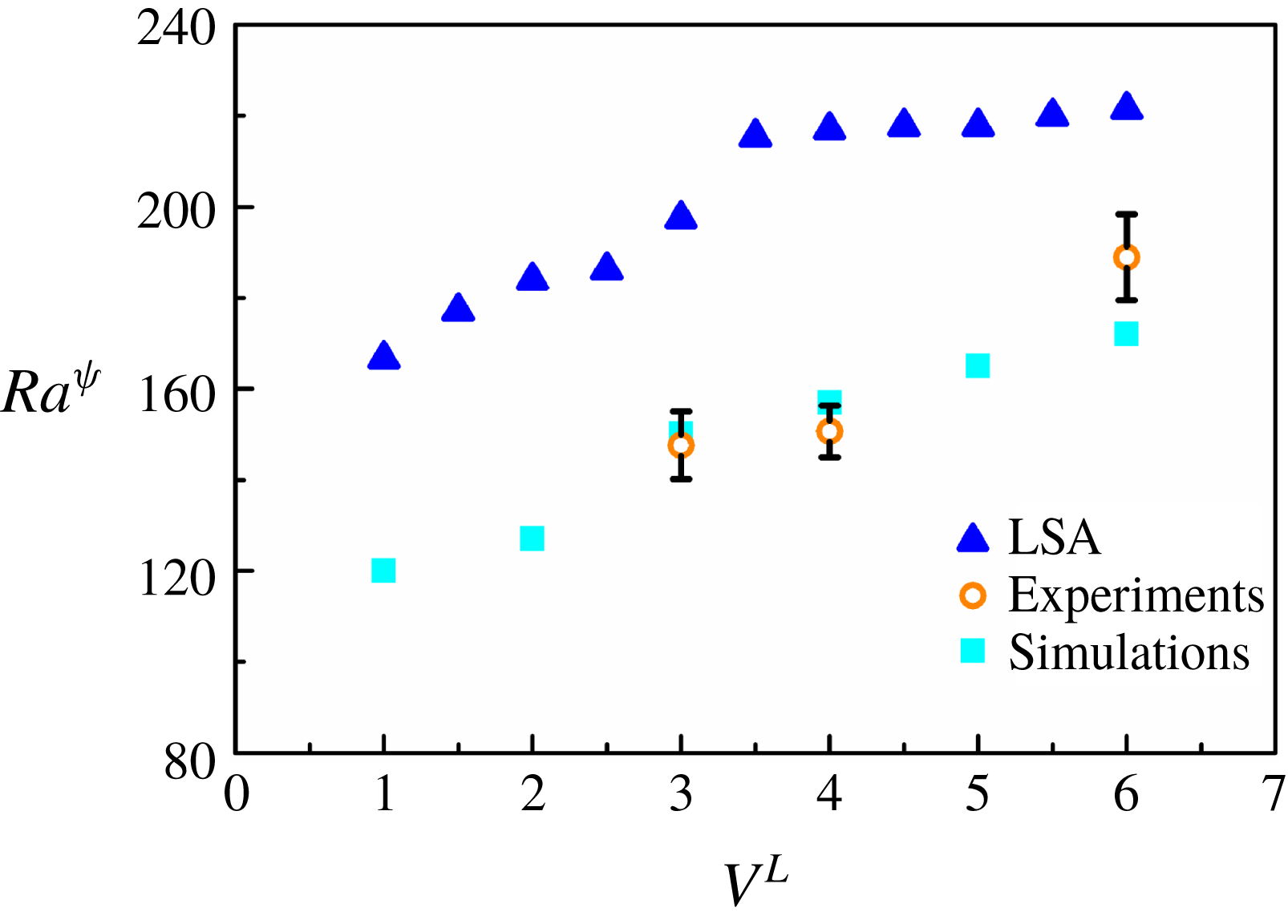
Figure 16. Variation of
 $Ra^{\unicode[STIX]{x1D713}}$
with
$Ra^{\unicode[STIX]{x1D713}}$
with
 $V^{L}$
depicted by LSA, experiments and numerical simulations. The other parameters used for LSA are
$V^{L}$
depicted by LSA, experiments and numerical simulations. The other parameters used for LSA are
 $h=-0.6$
,
$h=-0.6$
,
 $\unicode[STIX]{x1D6FF}=0.04$
,
$\unicode[STIX]{x1D6FF}=0.04$
,
 $K^{L}=0$
,
$K^{L}=0$
,
 $E^{L}=0$
,
$E^{L}=0$
,
 $Sc=500$
and
$Sc=500$
and
 $Re=0.5$
. The other parameters used for simulations are
$Re=0.5$
. The other parameters used for simulations are
 $K^{L}=0$
,
$K^{L}=0$
,
 $E^{L}=0$
,
$E^{L}=0$
,
 $Sc=500$
and
$Sc=500$
and
 $Re=0.5$
. The experimental values denote benzene–oleic acid (
$Re=0.5$
. The experimental values denote benzene–oleic acid (
 $V^{L}=3$
), benzene–soybean oil (
$V^{L}=3$
), benzene–soybean oil (
 $V^{L}=4$
) and benzene–silicone oil (
$V^{L}=4$
) and benzene–silicone oil (
 $V^{L}=6$
) fluid pairs. The average
$V^{L}=6$
) fluid pairs. The average
 $Re$
maintained during the experiments was 0.5. The error bars represent the standard deviations of three experiments.
$Re$
maintained during the experiments was 0.5. The error bars represent the standard deviations of three experiments.
Figure 17. (a) Shows the experimental snapshots of a silicone oil–benzene system under application of an electric field of
 $9.5~\text{kV}~\text{cm}^{-1}$
at different time instances. (b) Demonstrates the variation of experimental and theoretical wave speeds (
$9.5~\text{kV}~\text{cm}^{-1}$
at different time instances. (b) Demonstrates the variation of experimental and theoretical wave speeds (
 $v_{w}$
,
$v_{w}$
,
 $c_{r}$
) and wavelengths (
$c_{r}$
) and wavelengths (
 $\unicode[STIX]{x1D706}$
) with increasing electric field intensity (
$\unicode[STIX]{x1D706}$
) with increasing electric field intensity (
 $\boldsymbol{E}$
). The hollow symbols (blue) denote the values of the wavelengths, whereas the solid symbols (red) denote the wave speeds. The theoretical parameters used for the plot are
$\boldsymbol{E}$
). The hollow symbols (blue) denote the values of the wavelengths, whereas the solid symbols (red) denote the wave speeds. The theoretical parameters used for the plot are
 $h=-0.6$
,
$h=-0.6$
,
 $\unicode[STIX]{x1D6FF}=0.02$
,
$\unicode[STIX]{x1D6FF}=0.02$
,
 $Sc=500$
and
$Sc=500$
and
 $V^{L}=6$
. The error bars in the experimental points are twice the standard deviations obtained from three experiments. The average
$V^{L}=6$
. The error bars in the experimental points are twice the standard deviations obtained from three experiments. The average
 $Re$
maintained during the experiments was 0.5. (a) Corresponds to the top view of the flow configuration. In the image the top (bottom) layer corresponds to benzene (silicone oil) while in reality they flowed side by side. The videos were recorded at 500 fps under 2.5
$Re$
maintained during the experiments was 0.5. (a) Corresponds to the top view of the flow configuration. In the image the top (bottom) layer corresponds to benzene (silicone oil) while in reality they flowed side by side. The videos were recorded at 500 fps under 2.5
 $\times$
magnification. The arrow in (a) indicates the direction of the flow.
$\times$
magnification. The arrow in (a) indicates the direction of the flow.

Figure 18. Experimental micrographs showing the response of a stratified flow of a benzene–silicone oil system through the channel under application of ramp electric fields of strengths (a) 0–300 V, (b) 300–600 V, (c) 600–900 V and (d) 900–1500 V. The first image in the image set (a) corresponds to the system under 0 V electric field potential. Four regimes were distinguished, namely I, II, III and IV, as shown on the image sets. The applied voltage was gradually increased from 0 V–1500 V in 20 s, allowing 5 s for stabilization. Experiments were viewed with the help of a microscope under 2.5
 $\times$
magnification under the transmission mode. The videos were recorded at 500 fps. The images correspond to the top view of the flow configuration. The top layer corresponds to benzene and the bottom layer corresponds to silicone oil. The average
$\times$
magnification under the transmission mode. The videos were recorded at 500 fps. The images correspond to the top view of the flow configuration. The top layer corresponds to benzene and the bottom layer corresponds to silicone oil. The average
 $Re$
maintained during the experiments was 0.5. The arrow indicates the direction of the flow.
$Re$
maintained during the experiments was 0.5. The arrow indicates the direction of the flow.
Figure 17(a) shows experimental snapshots of the top view of the instabilities of a benzene–silicone oil system at different time intervals when exposed to an electric field potential of 400 V (
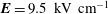 $\boldsymbol{E}=9.5~\text{kV}~\text{cm}^{-1}$
). Again, it may be noted here that the top layer shown in the image is benzene while the bottom one is silicone oil. However, in reality, the fluids flowed side by side while the images were taken from the top. The images show the progressive linear undulations near the interface and subsequent travelling waves towards the downstream of the channel under exposure to the electric field. Figure 17(b) shows a comparison between the theoretically calculated wavelengths (
$\boldsymbol{E}=9.5~\text{kV}~\text{cm}^{-1}$
). Again, it may be noted here that the top layer shown in the image is benzene while the bottom one is silicone oil. However, in reality, the fluids flowed side by side while the images were taken from the top. The images show the progressive linear undulations near the interface and subsequent travelling waves towards the downstream of the channel under exposure to the electric field. Figure 17(b) shows a comparison between the theoretically calculated wavelengths (
 $\unicode[STIX]{x1D706}$
) and wave speeds (
$\unicode[STIX]{x1D706}$
) and wave speeds (
 $c_{r}$
), and their corresponding experimental values. In order to experimentally measure the wavelength and wave speed of the unstable waves, the system was subjected to DC electric fields before the response was recorded. The frames extracted from the videos were then analysed to measure the required quantities. The wave speed was measured by tracking a wave over a particular distance towards the downstream, and then estimating the time required for the motion, as shown by the boxes in figure 17(a).
$c_{r}$
), and their corresponding experimental values. In order to experimentally measure the wavelength and wave speed of the unstable waves, the system was subjected to DC electric fields before the response was recorded. The frames extracted from the videos were then analysed to measure the required quantities. The wave speed was measured by tracking a wave over a particular distance towards the downstream, and then estimating the time required for the motion, as shown by the boxes in figure 17(a).
The experimental wavelength and wave speed were compared with the wavelength and speed of the E-I-mode obtained from linear stability analysis. It can be seen from figure 17(b) that the experimental and theoretical wavelengths are of the order of
 ${\sim}10^{-2}~\text{cm}$
, while the wave speeds are found to be of the order of
${\sim}10^{-2}~\text{cm}$
, while the wave speeds are found to be of the order of
 ${\sim}10^{-1}~\text{cm}~\text{s}^{-1}$
. The plot also shows that the wavelengths obtained from the experimental and theoretical analyses show the same qualitative decreasing trend, whereas the wave speeds exhibit an increasing trend, with an increase in the strength of the applied electric field. Again, the plot shows that the experimentally observed quantities are slightly different from the values predicted theoretically, which can be attributed to the various factors mentioned previously.
${\sim}10^{-1}~\text{cm}~\text{s}^{-1}$
. The plot also shows that the wavelengths obtained from the experimental and theoretical analyses show the same qualitative decreasing trend, whereas the wave speeds exhibit an increasing trend, with an increase in the strength of the applied electric field. Again, the plot shows that the experimentally observed quantities are slightly different from the values predicted theoretically, which can be attributed to the various factors mentioned previously.
4.4 Experimental and simulation results: nonlinear, time-periodic and unsteady regimes
Apart from the unstable linear modes, the experiments also uncovered the presence of interesting nonlinear, time-periodic and unsteady regimes in the two-layer stratified flow of miscible fluids under the influence of external EHD field inside a microchannel. In this section, we investigate the various flow patterns obtained during electroconvection when the applied field intensity is on the higher side. Upon application of electric potential to the system after development of a steady flow profile, four distinctive disturbance patterns are observed in the system, as demonstrated in figure 18. The image sets in figure 18(a–d) qualitatively identify these instability regimes, labelled as I, II, III and IV, as observed upon application of electric field from 0 to
 $35~\text{kV}~\text{cm}^{-1}$
. In these images the layer shown at the top (bottom) corresponds to benzene (silicone oil). In these experiments, the voltage was ramped up in 20 s in such a manner that the four quarters correspond to ramps of 0–300 V, 300–600 V, 600–900 V, 900–1500 V, respectively. The image set shown in figure 18(a) corresponds to the regime I, which is in response to the application of 0–300 V electric potential. In this regime, upon crossing a threshold voltage, the linear instability is first triggered in the less viscous fluid layer, which grows with the increase in the applied voltage. The characteristics of the instabilities in this regime have already been discussed in the previous sections. It may be noted here that these instabilities are reversible in nature because turning off the electric field again leads to the formation of the two-layer stratified flow in a short time. The image set in figure 18(b) and supporting movie 2 correspond to the regime II, obtained during application of 300–600 V electric potential. This regime is marked by the generation of repeated instability patterns at the downstream of the channel, which qualitatively resemble the time-periodic von Kármán vortex street in appearance. Upon further increase in voltage from 600–900 V, regime III is identified, as shown in the image set in figure 18(c) and supporting movie 3. In this situation, the time-periodic flow patterns start mixing with each other, in addition to having a smaller length scale and higher frequency of ejection of flow structures as compared to regime II. Finally, the voltage increment in the range of 900–1500 V, results in regime IV, depicted in the image set of figure 18(d) and supporting movie 4. The images illustrate the onset of a chaotic regime of flow instability where the periodic ejections of flow patterns having higher frequency and smaller length scale intermix to stimulate a ready mixing of the miscible layers.
$35~\text{kV}~\text{cm}^{-1}$
. In these images the layer shown at the top (bottom) corresponds to benzene (silicone oil). In these experiments, the voltage was ramped up in 20 s in such a manner that the four quarters correspond to ramps of 0–300 V, 300–600 V, 600–900 V, 900–1500 V, respectively. The image set shown in figure 18(a) corresponds to the regime I, which is in response to the application of 0–300 V electric potential. In this regime, upon crossing a threshold voltage, the linear instability is first triggered in the less viscous fluid layer, which grows with the increase in the applied voltage. The characteristics of the instabilities in this regime have already been discussed in the previous sections. It may be noted here that these instabilities are reversible in nature because turning off the electric field again leads to the formation of the two-layer stratified flow in a short time. The image set in figure 18(b) and supporting movie 2 correspond to the regime II, obtained during application of 300–600 V electric potential. This regime is marked by the generation of repeated instability patterns at the downstream of the channel, which qualitatively resemble the time-periodic von Kármán vortex street in appearance. Upon further increase in voltage from 600–900 V, regime III is identified, as shown in the image set in figure 18(c) and supporting movie 3. In this situation, the time-periodic flow patterns start mixing with each other, in addition to having a smaller length scale and higher frequency of ejection of flow structures as compared to regime II. Finally, the voltage increment in the range of 900–1500 V, results in regime IV, depicted in the image set of figure 18(d) and supporting movie 4. The images illustrate the onset of a chaotic regime of flow instability where the periodic ejections of flow patterns having higher frequency and smaller length scale intermix to stimulate a ready mixing of the miscible layers.
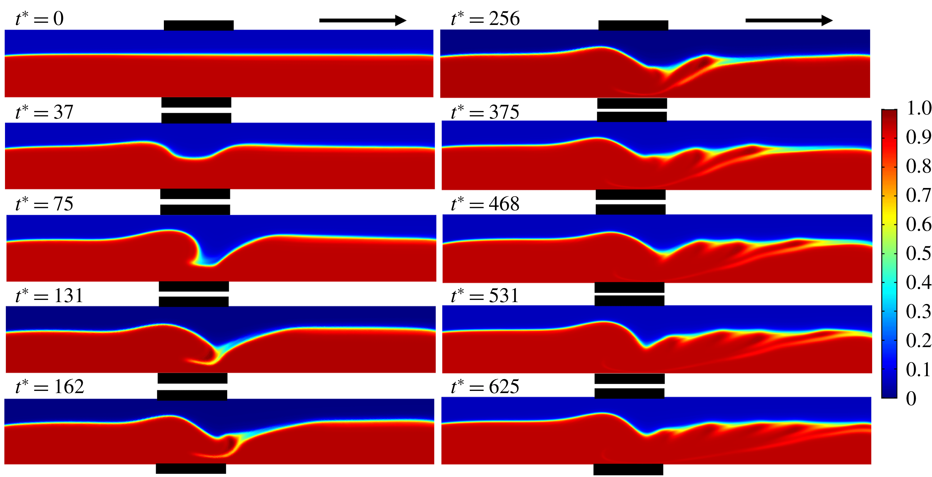
Figure 19. Computational snapshots showing the concentration surface plot of a stratified flow of benzene–silicone oil (
 $V^{L}=6$
) through the channel at
$V^{L}=6$
) through the channel at
 $Ra^{\unicode[STIX]{x1D713}}=225$
. Here,
$Ra^{\unicode[STIX]{x1D713}}=225$
. Here,
 $t^{\ast }$
represents non-dimensional time. The other parameters used for the simulation are
$t^{\ast }$
represents non-dimensional time. The other parameters used for the simulation are
 $K^{L}=-4$
,
$K^{L}=-4$
,
 $E^{L}=-0.15$
,
$E^{L}=-0.15$
,
 $Sc=700$
,
$Sc=700$
,
 $I^{q}=1$
and
$I^{q}=1$
and
 $Re=0.5$
. The arrows in the images indicate the direction of the flow. The black rectangles outside the channel represent the electrodes. A positive potential is applied to the top electrode while the bottom electrode is grounded.
$Re=0.5$
. The arrows in the images indicate the direction of the flow. The black rectangles outside the channel represent the electrodes. A positive potential is applied to the top electrode while the bottom electrode is grounded.
The CFD simulations also predict qualitatively similar flow structures upon application of an electric field to a stratified flow of two miscible fluids through a channel. Figure 19 and supporting movie 6 depict the concentration surface plot of a stratified flow of benzene–silicone oil (
 $V^{L}=6$
) at
$V^{L}=6$
) at
 $Ra^{\unicode[STIX]{x1D713}}=225$
. The flow is undisturbed at
$Ra^{\unicode[STIX]{x1D713}}=225$
. The flow is undisturbed at
 $t^{\ast }=0$
in the absence of an electric field. The EHD instability sets into the system upon application of an electric field, and a vortex street similar to the experimental regimes II and III have been observed in figure 19. The simulations mimic the experimental findings of the reduction of the size and time scale of vortex generation on increasing the electric field, which is depicted in figure 20. The figure shows the concentration surface plots of the benzene–silicone oil system at different values of
$t^{\ast }=0$
in the absence of an electric field. The EHD instability sets into the system upon application of an electric field, and a vortex street similar to the experimental regimes II and III have been observed in figure 19. The simulations mimic the experimental findings of the reduction of the size and time scale of vortex generation on increasing the electric field, which is depicted in figure 20. The figure shows the concentration surface plots of the benzene–silicone oil system at different values of
 $Ra^{\unicode[STIX]{x1D713}}$
. It can be seen from the figure that the sizes of the vortices decrease on increasing
$Ra^{\unicode[STIX]{x1D713}}$
. It can be seen from the figure that the sizes of the vortices decrease on increasing
 $Ra^{\unicode[STIX]{x1D713}}$
from 225 to 450, accompanied by an increase in the frequency of vortex shedding. This behaviour is qualitatively similar to the experimental observations reported in figure 18. It may be noted here that the simulation results are reproducible with other fluid pairs (different
$Ra^{\unicode[STIX]{x1D713}}$
from 225 to 450, accompanied by an increase in the frequency of vortex shedding. This behaviour is qualitatively similar to the experimental observations reported in figure 18. It may be noted here that the simulation results are reproducible with other fluid pairs (different
 $V^{L}$
) and also considering liquids with equal ionic mobility (
$V^{L}$
) and also considering liquids with equal ionic mobility (
 $K^{L}=0$
), however, the results are not discussed here for the sake of brevity and two such cases are depicted in supporting movies 7 and 8.
$K^{L}=0$
), however, the results are not discussed here for the sake of brevity and two such cases are depicted in supporting movies 7 and 8.
In order to characterize regimes II and III shown in figure 18, the frequency of vortex shedding is correlated with the strength of the applied electric field. For this purpose, we analyse the variation of Strouhal number (
 $St$
) with electric field Rayleigh number (
$St$
) with electric field Rayleigh number (
 $Ra^{\unicode[STIX]{x1D713}}$
). The experimental Strouhal number (
$Ra^{\unicode[STIX]{x1D713}}$
). The experimental Strouhal number (
 $St$
) is defined as
$St$
) is defined as
 $St=fR/U$
, where
$St=fR/U$
, where
 $f$
is the frequency of shedding,
$f$
is the frequency of shedding,
 $R$
is the characteristic length and
$R$
is the characteristic length and
 $U$
is the average flow velocity. In these experiments, the benzene–silicone oil system was subjected to a DC voltage input in the range of 300–850 V at increments of 50 V. The system responded with the generation of vortices, which were recorded and analysed simultaneously. The frequency of the vortex cycles generated per second (f) at each of the applied electric fields was calculated from the frames extracted from the recorded videos. Figure 21 shows the variation of
$U$
is the average flow velocity. In these experiments, the benzene–silicone oil system was subjected to a DC voltage input in the range of 300–850 V at increments of 50 V. The system responded with the generation of vortices, which were recorded and analysed simultaneously. The frequency of the vortex cycles generated per second (f) at each of the applied electric fields was calculated from the frames extracted from the recorded videos. Figure 21 shows the variation of
 $St$
with
$St$
with
 $Ra^{\unicode[STIX]{x1D713}}$
, for regimes II and III. The figure suggests that for both regimes II and III, the frequency of vortex generation increases (increasing
$Ra^{\unicode[STIX]{x1D713}}$
, for regimes II and III. The figure suggests that for both regimes II and III, the frequency of vortex generation increases (increasing
 $St$
) with the strength of the applied field (increasing
$St$
) with the strength of the applied field (increasing
 $Ra^{\unicode[STIX]{x1D713}}$
). The higher values of
$Ra^{\unicode[STIX]{x1D713}}$
). The higher values of
 $St$
in regime III indicate larger frequencies of the vortices as compared to regime II, which can be attributed to a higher electrical force in regime III compared to regime II. Further, regimes II and III can also be differentiated by an abrupt jump observed in the values of
$St$
in regime III indicate larger frequencies of the vortices as compared to regime II, which can be attributed to a higher electrical force in regime III compared to regime II. Further, regimes II and III can also be differentiated by an abrupt jump observed in the values of
 $St$
. Interestingly, the experimental time scale of vortex generation,
$St$
. Interestingly, the experimental time scale of vortex generation,
 $t_{v}\sim O(10^{-2}\;\text{s})$
, is found to be very close to the theoretical one,
$t_{v}\sim O(10^{-2}\;\text{s})$
, is found to be very close to the theoretical one,
 $t_{v}\sim O(10^{-2}\;\text{s})\sim (RV^{L}\unicode[STIX]{x1D702}_{1})/(K\unicode[STIX]{x1D713}_{0}U)$
.
$t_{v}\sim O(10^{-2}\;\text{s})\sim (RV^{L}\unicode[STIX]{x1D702}_{1})/(K\unicode[STIX]{x1D713}_{0}U)$
.
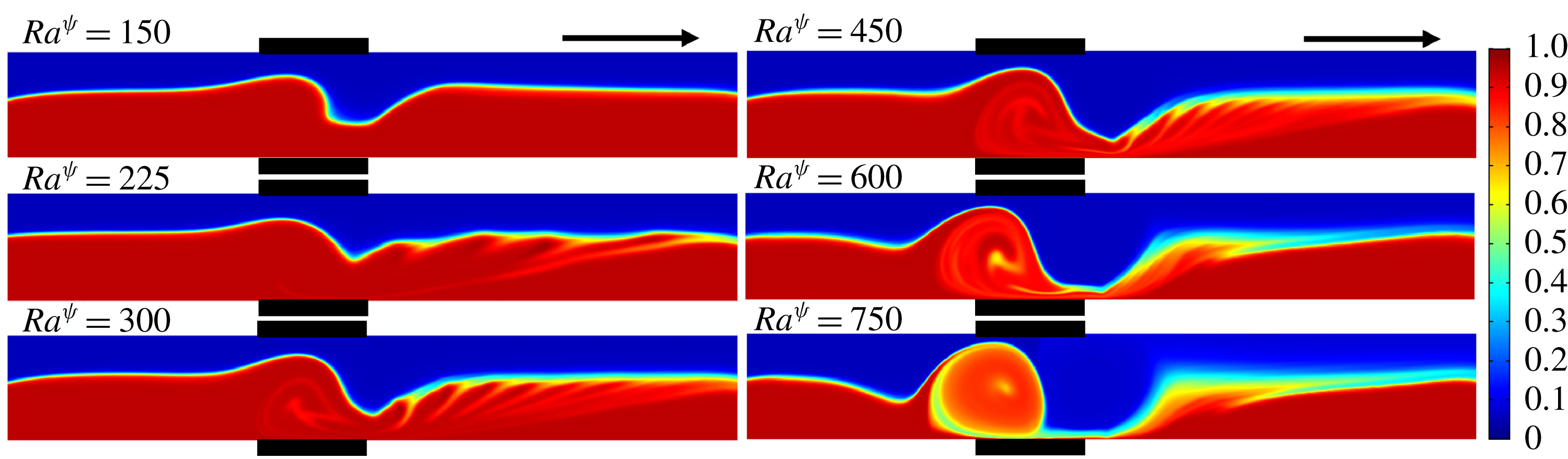
Figure 20. Computational snapshots showing the concentration surface plot of a stratified flow of benzene–silicone oil (
 $V^{L}=6$
) through the channel at different values of
$V^{L}=6$
) through the channel at different values of
 $Ra^{\unicode[STIX]{x1D713}}$
at
$Ra^{\unicode[STIX]{x1D713}}$
at
 $t^{\ast }=300$
. It may be noted here that
$t^{\ast }=300$
. It may be noted here that
 $t$
is normalized considering
$t$
is normalized considering
 $\unicode[STIX]{x1D6F9}_{0}=300$
V to maintain uniformity in reporting the results. The other parameters used for the simulation are
$\unicode[STIX]{x1D6F9}_{0}=300$
V to maintain uniformity in reporting the results. The other parameters used for the simulation are
 $K^{L}=-4$
,
$K^{L}=-4$
,
 $E^{L}=-0.15$
,
$E^{L}=-0.15$
,
 $Sc=700$
,
$Sc=700$
,
 $I^{q}=1$
and
$I^{q}=1$
and
 $Re=0.5$
. The arrows in the images indicate the direction of the flow. The black rectangles outside the channel represent the locations of the electrodes. A positive potential is applied to the top electrode while the bottom electrode is grounded.
$Re=0.5$
. The arrows in the images indicate the direction of the flow. The black rectangles outside the channel represent the locations of the electrodes. A positive potential is applied to the top electrode while the bottom electrode is grounded.
We introduce a parameter
 $\unicode[STIX]{x1D709}$
to quantify the amount of perturbation instilled into the system upon application of electric fields of varying strengths for the regimes I–IV, discussed in figure 18. For this purpose, initially, the benzene–silicone oil system was subjected to DC voltage application in the range of 0–1500 V, at increments of 50 V, and the response was recorded simultaneously. We define,
$\unicode[STIX]{x1D709}$
to quantify the amount of perturbation instilled into the system upon application of electric fields of varying strengths for the regimes I–IV, discussed in figure 18. For this purpose, initially, the benzene–silicone oil system was subjected to DC voltage application in the range of 0–1500 V, at increments of 50 V, and the response was recorded simultaneously. We define,
 $\unicode[STIX]{x1D709}=1-I_{e}/I_{i}$
, where
$\unicode[STIX]{x1D709}=1-I_{e}/I_{i}$
, where
 $I_{i}$
is the mean grey scale level in absence of an electric field and
$I_{i}$
is the mean grey scale level in absence of an electric field and
 $I_{e}$
is the mean grey scale level in the presence of an electric field. The parameter
$I_{e}$
is the mean grey scale level in the presence of an electric field. The parameter
 $\unicode[STIX]{x1D709}_{N}$
represents the normalized values of
$\unicode[STIX]{x1D709}_{N}$
represents the normalized values of
 $\unicode[STIX]{x1D709}$
, obtained by dividing the latter by the maximum value of
$\unicode[STIX]{x1D709}$
, obtained by dividing the latter by the maximum value of
 $\unicode[STIX]{x1D709}$
. The grey scale intensities were measured by image analysis of the extracted frames using the commercial software MATLAB. Figure 22(a) shows the variation of
$\unicode[STIX]{x1D709}$
. The grey scale intensities were measured by image analysis of the extracted frames using the commercial software MATLAB. Figure 22(a) shows the variation of
 $\unicode[STIX]{x1D709}_{N}$
with
$\unicode[STIX]{x1D709}_{N}$
with
 $Ra^{\unicode[STIX]{x1D713}}$
. The
$Ra^{\unicode[STIX]{x1D713}}$
. The
 $\unicode[STIX]{x1D709}_{N}$
in this plot were calculated for three distinct regions marked 1, 2 and 3, located upstream, within and downstream of the area of application of the electric field, respectively, as shown in the plot by the rectangular boxes. The intensity values represent the mean intensity of all the pixels contained within the regions of interest namely, regions 1, 2 and 3.
$\unicode[STIX]{x1D709}_{N}$
in this plot were calculated for three distinct regions marked 1, 2 and 3, located upstream, within and downstream of the area of application of the electric field, respectively, as shown in the plot by the rectangular boxes. The intensity values represent the mean intensity of all the pixels contained within the regions of interest namely, regions 1, 2 and 3.
Figure 21. Variation of Strouhal number (
 $St$
) with electric field Rayleigh number (
$St$
) with electric field Rayleigh number (
 $Ra^{\unicode[STIX]{x1D713}}$
) in regimes II and III, for a benzene–silicone oil system under DC voltage input. The average
$Ra^{\unicode[STIX]{x1D713}}$
) in regimes II and III, for a benzene–silicone oil system under DC voltage input. The average
 $Re$
maintained during the experiments was 0.5. The arrow indicates the direction of the flow.
$Re$
maintained during the experiments was 0.5. The arrow indicates the direction of the flow.
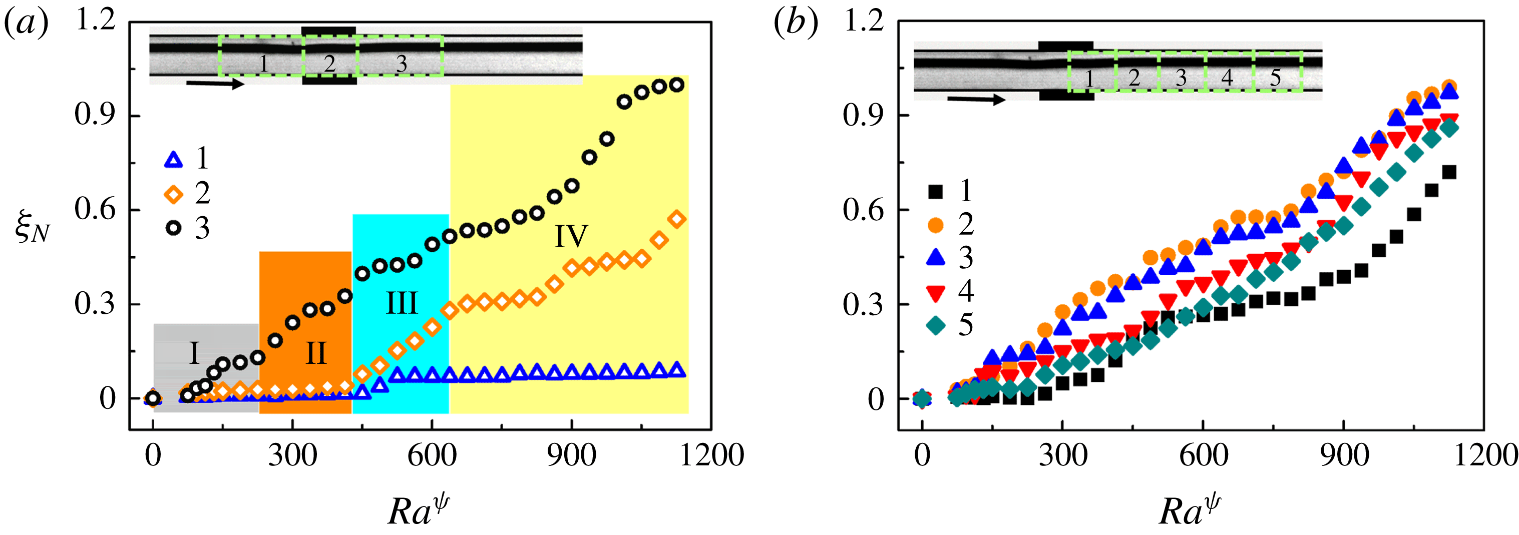
Figure 22. (a,b) Show the variation of perturbation parameter
 $\unicode[STIX]{x1D709}_{N}$
with
$\unicode[STIX]{x1D709}_{N}$
with
 $Ra^{\unicode[STIX]{x1D713}}$
. (a) The three regions 1, 2 and 3 in the inset are located at the upstream, within and downstream, of the region where the electric field was applied, respectively. In (b), five regions, 1–5, in the inset are identified in the downstream of the region of application of electric field. Regions 1 and 3 in (a) are two channels widths in length, and one channel width in breadth. All other regions are squares of one channel width side. The system studied was that of benzene–silicone oil, under application of DC voltages. The average
$Ra^{\unicode[STIX]{x1D713}}$
. (a) The three regions 1, 2 and 3 in the inset are located at the upstream, within and downstream, of the region where the electric field was applied, respectively. In (b), five regions, 1–5, in the inset are identified in the downstream of the region of application of electric field. Regions 1 and 3 in (a) are two channels widths in length, and one channel width in breadth. All other regions are squares of one channel width side. The system studied was that of benzene–silicone oil, under application of DC voltages. The average
 $Re$
maintained during the experiments was 0.5. The arrow indicates the direction of the flow.
$Re$
maintained during the experiments was 0.5. The arrow indicates the direction of the flow.
The plot suggests that, while
 $\unicode[STIX]{x1D709}_{N}$
remains nearly constant at the upstream of the electrodes, the same increases with an increase in
$\unicode[STIX]{x1D709}_{N}$
remains nearly constant at the upstream of the electrodes, the same increases with an increase in
 $Ra^{\unicode[STIX]{x1D713}}$
within the electrode and downstream regions. Further, at lower values of
$Ra^{\unicode[STIX]{x1D713}}$
within the electrode and downstream regions. Further, at lower values of
 $Ra^{\unicode[STIX]{x1D713}}$
, when there is little perturbation in the system, the grey scale levels do not change significantly, yielding lower values of
$Ra^{\unicode[STIX]{x1D713}}$
, when there is little perturbation in the system, the grey scale levels do not change significantly, yielding lower values of
 $\unicode[STIX]{x1D709}_{N}$
. With the increase in
$\unicode[STIX]{x1D709}_{N}$
. With the increase in
 $Ra^{\unicode[STIX]{x1D713}}$
, the development of the instability modes yield higher values of
$Ra^{\unicode[STIX]{x1D713}}$
, the development of the instability modes yield higher values of
 $\unicode[STIX]{x1D709}_{N}$
. Region 3 in the downstream, where all the unstable perturbations travel with the fluid, shows a more rapid increase in the values of
$\unicode[STIX]{x1D709}_{N}$
. Region 3 in the downstream, where all the unstable perturbations travel with the fluid, shows a more rapid increase in the values of
 $\unicode[STIX]{x1D709}_{N}$
with
$\unicode[STIX]{x1D709}_{N}$
with
 $Ra^{\unicode[STIX]{x1D713}}$
, as compared to regions 1 and 2. Further, regions 2 and 3 show significantly higher values of
$Ra^{\unicode[STIX]{x1D713}}$
, as compared to regions 1 and 2. Further, regions 2 and 3 show significantly higher values of
 $\unicode[STIX]{x1D709}_{N}$
in instability regimes III and IV owing to the chaotic nature of the instabilities. Figure 22(b) shows the variation of
$\unicode[STIX]{x1D709}_{N}$
in instability regimes III and IV owing to the chaotic nature of the instabilities. Figure 22(b) shows the variation of
 $\unicode[STIX]{x1D709}_{N}$
with
$\unicode[STIX]{x1D709}_{N}$
with
 $Ra^{\unicode[STIX]{x1D713}}$
in five different regions immediately downstream to the electrode region, as shown by boxes in the figure. The figure suggests that
$Ra^{\unicode[STIX]{x1D713}}$
in five different regions immediately downstream to the electrode region, as shown by boxes in the figure. The figure suggests that
 $\unicode[STIX]{x1D709}_{N}$
is minimum near region 1, then increases sharply in regions 2 and 3 before again reducing in regions 4 and 5. The plots infer that perturbation strength is maximum in region 2, which is the immediate downstream of the region of application of electric force. The image suggests that the electric field induced perturbations in these systems can only grow up to a certain part of the downstream of the electrodes before they are transported downstream due to pressure-driven flow of the fluid layers. It is important to note here that
$\unicode[STIX]{x1D709}_{N}$
is minimum near region 1, then increases sharply in regions 2 and 3 before again reducing in regions 4 and 5. The plots infer that perturbation strength is maximum in region 2, which is the immediate downstream of the region of application of electric force. The image suggests that the electric field induced perturbations in these systems can only grow up to a certain part of the downstream of the electrodes before they are transported downstream due to pressure-driven flow of the fluid layers. It is important to note here that
 $\unicode[STIX]{x1D709}_{N}$
is also a measure of mixing of the fluids in the downstream of the channel. A higher value of
$\unicode[STIX]{x1D709}_{N}$
is also a measure of mixing of the fluids in the downstream of the channel. A higher value of
 $\unicode[STIX]{x1D709}_{N}$
signifies a larger amount of mixing between the layers. Thus, both the plots in figure 22 suggest that the increase in the electric field intensity can cause a rapid mixing of the fluids at the immediate downstream of the channel. Further, the plots also suggest that the mixing length reduces with the increase in field intensity. The experiments also show that the liquid can immediately be de-mixed when the electric field is turned off, i.e. the perturbations die out immediately upon removal of electric field.
$\unicode[STIX]{x1D709}_{N}$
signifies a larger amount of mixing between the layers. Thus, both the plots in figure 22 suggest that the increase in the electric field intensity can cause a rapid mixing of the fluids at the immediate downstream of the channel. Further, the plots also suggest that the mixing length reduces with the increase in field intensity. The experiments also show that the liquid can immediately be de-mixed when the electric field is turned off, i.e. the perturbations die out immediately upon removal of electric field.
Figures 18–22 show the EHD induced steady, time-periodic and chaotic instabilities in a pressure-driven viscosity stratified flow of a pair of miscible fluids inside a microchannel, which can be employed for rapid mixing of the fluids inside microfluidic devices. The method is found to be reversible in nature because immediate de-mixing of the layers takes place upon the removal of the electric field influence.
Figure 23 and supporting movie 5 show the use of multiple electrodes to cause a rapid mixing of the miscible fluids undergoing a stratified flow inside a microchannel. The optical micrographs (a–f) show the response of a benzene–silicone oil stratified flow when a DC voltage of 0–500 V is ramped up through five pairs of electrodes integrated in a staggered manner along the microchannel wall, as shown in the figure. The electrode separation distance in these experiments has been optimized based on the observations made with the single electrode experiments. Again, the top (bottom) layer shown in the image corresponds to benzene (silicone oil). In these experiments, the voltage was ramped up in 5 s to cause the phenomena. All the frames shown in this figure have been extracted from the supporting movie 5. Panel (a) corresponds to the pressure-driven situation in absence of the electric field while (b) shows the onset of the electric field induced mixing. Panels (c–f) show the progressive reduction in the mixing length owing to the generation of time-periodic and unsteady flow patterns with the progressive increase in the field intensity. The multiple electrode arrangement ensure an amplified perturbation in this system induced by the electric field as compared to a single electrode system. Thus, a more efficient mixing of the fluids can be achieved at a much lower voltage in the multi-electrode system. The figure shows the use of the proposed methodology to rapidly mix fluids layers inside the microfluidic devices.
5 Conclusions
A combined theoretical and experimental study uncovers the salient features of electric field induced instabilities associated with the viscosity stratified flow of a pair of miscible fluids inside microchannels. The major conclusions are:
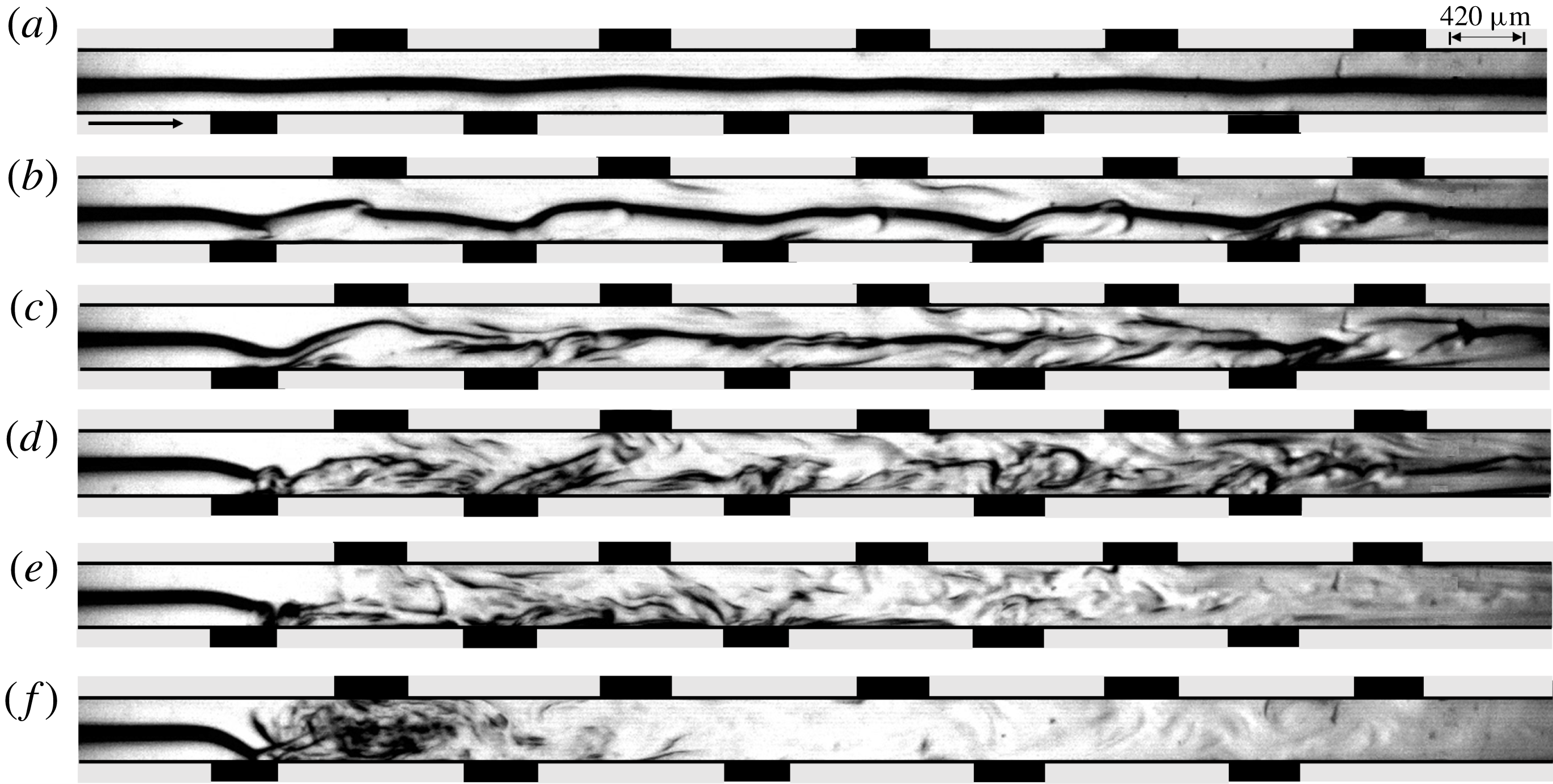
Figure 23. Experimental micrographs (a–f) show the response of a benzene–silicone oil stratified flow upon application of ramp DC voltage of 0–500 V, through five pairs of electrodes integrated along the channel wall in a staggered fashion. The images correspond to the top view of the flow configuration. The top layer corresponds to benzene and the bottom layer corresponds to silicone oil. (a) Corresponds to the system at 0 V. The average
 $Re$
maintained during the experiments was 0.5.
$Re$
maintained during the experiments was 0.5.
(i) A general linear stability analysis reveals that the EHD instabilities of such systems appear only beyond a critical field intensity. The analysis also uncovers the presence of five distinctive instability modes, which are identified as electric field mode I (E-I), electric field mode II (E-II), viscous mode (V), diffusive mode (D) and the K-mode. Mode E-I appears in the bulk of the lower viscosity fluid at the lower values of
 $Ra^{\unicode[STIX]{x1D713}}$
while the E-II-mode manifests in the higher viscosity fluid at very high values of
$Ra^{\unicode[STIX]{x1D713}}$
. The V-mode appears when the viscosity difference between the fluids is high. Presence of the electric field facilitates the onset of the V-mode when compared with the regular pressure driven flows. The D-mode appears in the mixed interfacial region at higher values of
$Sc$
due to steep variation of perturbation concentration across the interface. Again, the presence of the electric field facilitates the onset of the D-mode when compared with the regular pressure-driven flows. A contrast of the ionic mobility in the fluids cause the appearance of the much shorter wavelength K-mode.
$Ra^{\unicode[STIX]{x1D713}}$
while the E-II-mode manifests in the higher viscosity fluid at very high values of
$Ra^{\unicode[STIX]{x1D713}}$
. The V-mode appears when the viscosity difference between the fluids is high. Presence of the electric field facilitates the onset of the V-mode when compared with the regular pressure driven flows. The D-mode appears in the mixed interfacial region at higher values of
$Sc$
due to steep variation of perturbation concentration across the interface. Again, the presence of the electric field facilitates the onset of the D-mode when compared with the regular pressure-driven flows. A contrast of the ionic mobility in the fluids cause the appearance of the much shorter wavelength K-mode.(ii) The location of the interface (h), thickness of the interface (
$\unicode[STIX]{x1D6FF}$
), level of charge injection (
$I^{q}$
), strength of the applied EHD field (
$Ra^{\unicode[STIX]{x1D713}}$
), viscosity contrast across the diffused interface (
$V^{L}$
) and diffusivity across the interface (
$Sc$
), are found to be some of the very important parameters for these types of instabilities. For relatively small variations in the dielectric constants of the fluids (
$E^{L}$
), the E-I-mode remains nearly unaffected. In particular, the E-I-mode and E-II-mode can be facilitated by increasing the applied field intensity, charge injection levels and reducing the overall viscosity of the fluids. In the linear regime, the experimental and theoretical values obtained for the critical electric field strength, wave speed and wavelength of the E-I-mode of instability are found to be in reasonable qualitative agreement.(iii) Experiments uncover four distinct regimes of instabilities. The linear regime I corresponds to the onset of instability waves beyond a critical field intensity. With further increase in the applied voltage, the regime II marks the initiation of the nonlinear regime with the appearance of time-periodic vortices in the downstream of the electrode region. On further increasing the electric field intensity a regime III appears where smaller vortices are generated at higher frequencies leading to intermixing of the flow patterns. The transition of regime II to regime III is marked by an abrupt jump in the Strouhal number. Two-dimensional nonlinear CFD simulations also predict the appearance of vortices which are qualitatively similar to the experimental observations of regime II and III. The simulated results show reduction in size and increment in frequency of shedding with the increase in the electric field intensity. At still higher field intensities, the flow becomes unstructured and chaotic in regime IV leading to total mixing of the two fluids downstream the region of application of electric potential.
(iv) From the perspective of mixing, among all the regimes, the chaotic regime IV with coherent flow patterns is found to be the most suitable one. The mixing is found to happen at the immediate downstream of the electrodes inserted in the channel where electric field can engender a strong intermixing of the layers. The mixing decreases at the far downstream of the channel due to viscous damping of the perturbations induced by the electric field. Interestingly, the mixing and de-mixing processes have been observed to be reversible because the flow immediately restores to its stratified configuration on switching off the electric field. The mixing efficiency is found to increase with the increase in the strength of the applied field and the number of electrodes inserted across the channel.


In summary, the study uncovers a pathway to integrate the influence of an external electrostatic field with a microfluidic device in order to remotely control the mixing of the fluid layers. The phenomenon can be of significance in improving the efficiency of multifarious cutting-edge microfluidic applications which include mixing, pumping, heat exchange, mass transfer and reaction engineering. In depth investigation of the coherent and chaotic regimes, along with a spatial stability analysis of the system has been kept as future scope of research work.
Acknowledgements
We thank DST SERB, grant no. EMR/2016/001824, MeitY-grant no. 5(9)/2012-NANO and the DST-FIST-grant SR/FST/ETII-028/2010, Government of India, for financial aids. We are also grateful for the support from the computer centre for the supercomputing PARAM Ishan facilities at IIT Guwahati. Discussions with Dr S. Timung and Mr J. Chaudhuri are also gratefully acknowledged.
Supplementary movies
Supplementary movies are available at https://doi.org/10.1017/jfm.2018.1023.
Appendix A. Energy analysis
The contributions of the various forces towards production or dissipation of the disturbance kinetic energy are analysed to obtain a more comprehensive understanding of the instability phenomenon. The energy equation is obtained by first multiplying the
 $x$
and
$x$
and
 $z$
directional momentum equations (3.3) with the complex conjugate of
$z$
directional momentum equations (3.3) with the complex conjugate of
 $\tilde{u}$
(
$\tilde{u}$
(
 $\tilde{u} ^{\dagger }$
) and
$\tilde{u} ^{\dagger }$
) and
 $\tilde{w}$
(
$\tilde{w}$
(
 $\tilde{w}^{\dagger }$
), respectively, then adding the equations, and subsequently, integrating them across the channel length (Selvam et al.
Reference Selvam, Merk, Govindarajan and Meiburg2007). The energy equation is given by,
$\tilde{w}^{\dagger }$
), respectively, then adding the equations, and subsequently, integrating them across the channel length (Selvam et al.
Reference Selvam, Merk, Govindarajan and Meiburg2007). The energy equation is given by,
 $$\begin{eqnarray}E_{KE}=E_{RS}+E_{VD}+E_{V}+E_{E},\end{eqnarray}$$
where,
 $E_{KE}$
represents the rate of change of disturbance kinetic energy,
$E_{KE}$
represents the rate of change of disturbance kinetic energy,
 $E_{RS}$
is the energy associated with the Reynolds stress,
$E_{RS}$
is the energy associated with the Reynolds stress,
 $E_{VD}$
is the viscous dissipation energy,
$E_{VD}$
is the viscous dissipation energy,
 $E_{V}$
is the rate of energy change due to viscosity stratification and
$E_{V}$
is the rate of energy change due to viscosity stratification and
 $E_{E}$
is the energy associated with the electrical field body force component in the momentum equation. Here,
$E_{E}$
is the energy associated with the electrical field body force component in the momentum equation. Here,
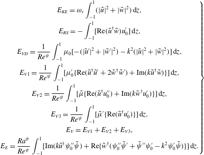 $$\begin{eqnarray}\left.\begin{array}{@{}c@{}}\displaystyle E_{KE}=\unicode[STIX]{x1D714}_{r}\int _{-1}^{1}(|\tilde{u} |^{2}+|\tilde{w}|^{2})\,\text{d}z,\\ \displaystyle E_{RS}=-\int _{-1}^{1}[\text{Re}(\tilde{u} ^{\dagger }\tilde{w})u_{0}^{\prime }]\,\text{d}z,\\ \displaystyle E_{VD}=\frac{1}{Re^{\unicode[STIX]{x1D713}}}\int _{-1}^{1}\unicode[STIX]{x1D707}_{0}[-(|\tilde{u} ^{\prime }|^{2}+|\tilde{w}^{\prime }|^{2})-k^{2}(|\tilde{u} |^{2}+|\tilde{w}|^{2})]\,\text{d}z,\\ \displaystyle E_{V1}=\frac{1}{Re^{\unicode[STIX]{x1D713}}}\int _{-1}^{1}[\unicode[STIX]{x1D707}_{0}^{\prime }\{\text{Re}(\tilde{u} ^{\dagger }\tilde{u} ^{\prime }+2\tilde{w}^{\dagger }\tilde{w}^{\prime })+\text{Im}(k\tilde{u} ^{\dagger }\tilde{w})\}]\,\text{d}z,\\ \displaystyle E_{V2}=\frac{1}{Re^{\unicode[STIX]{x1D713}}}\int _{-1}^{1}[\tilde{\unicode[STIX]{x1D707}}\{\text{Re}(\tilde{u} ^{\dagger }u_{0}^{\prime \prime })+\text{Im}(k\tilde{w}^{\dagger }u_{0}^{\prime })\}]\,\text{d}z,\\ \displaystyle E_{V3}=\frac{1}{Re^{\unicode[STIX]{x1D713}}}\int _{-1}^{1}[\tilde{\unicode[STIX]{x1D707}}^{\prime }\{\text{Re}(\tilde{u} ^{\dagger }u_{0}^{\prime })\}]\,\text{d}z,\\ \displaystyle E_{V}=E_{V1}+E_{V2}+E_{V3},\\ \displaystyle E_{E}=\frac{Ra^{\unicode[STIX]{x1D713}}}{Re^{\unicode[STIX]{x1D713}}}\int _{-1}^{1}[\text{Im}(k\tilde{u} ^{\dagger }\unicode[STIX]{x1D713}_{0}^{\prime \prime }\tilde{\unicode[STIX]{x1D713}})+\text{Re}\{\tilde{w}^{\dagger }(\unicode[STIX]{x1D713}_{0}^{\prime \prime }\tilde{\unicode[STIX]{x1D713}}^{\prime }+\tilde{\unicode[STIX]{x1D713}}^{\prime \prime }\unicode[STIX]{x1D713}_{0}^{\prime }-k^{2}\unicode[STIX]{x1D713}_{0}^{\prime }\tilde{\unicode[STIX]{x1D713}})\}]\,\text{d}z.\end{array}\right\}\end{eqnarray}$$
Appendix B. Three-dimensional stability analysis
The non-dimensional scheme is given by,
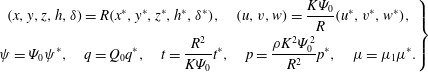 $$\begin{eqnarray}\left.\begin{array}{@{}c@{}}\displaystyle (x,y,z,h,\unicode[STIX]{x1D6FF})=R(x^{\ast },y^{\ast },z^{\ast },h^{\ast },\unicode[STIX]{x1D6FF}^{\ast }),\quad (u,\mathit{v},\mathit{w})=\frac{K\unicode[STIX]{x1D6F9}_{0}}{R}(u^{\ast },v^{\ast },w^{\ast }),\\ \displaystyle \unicode[STIX]{x1D713}=\unicode[STIX]{x1D6F9}_{0}\unicode[STIX]{x1D713}^{\ast },\quad q=Q_{0}q^{\ast },\quad t=\frac{R^{2}}{K\unicode[STIX]{x1D6F9}_{0}}t^{\ast },\quad p=\frac{\unicode[STIX]{x1D70C}K^{2}\unicode[STIX]{x1D6F9}_{0}^{2}}{R^{2}}p^{\ast },\quad \unicode[STIX]{x1D707}=\unicode[STIX]{x1D707}_{1}\unicode[STIX]{x1D707}^{\ast }.\end{array}\right\}\end{eqnarray}$$
Here,
 $u$
,
$u$
,
 $v$
and
$v$
and
 $w$
represent the
$w$
represent the
 $x$
,
$x$
,
 $y$
and
$y$
and
 $z$
directional velocity components, respectively. The normal linear modes represented by (3.19) are modified as,
$z$
directional velocity components, respectively. The normal linear modes represented by (3.19) are modified as,
 $$\begin{eqnarray}\displaystyle [u,v,w,p,\unicode[STIX]{x1D713},S,\unicode[STIX]{x1D707}](x,y,z,t) & = & \displaystyle [u_{0}(z),0,0,p_{0},\unicode[STIX]{x1D713}_{0}(z),S_{0}(z),\unicode[STIX]{x1D707}_{0}(z)]\nonumber\\ \displaystyle & & \displaystyle +\,[\tilde{u} ,\tilde{v},\tilde{w},\tilde{p},\tilde{\unicode[STIX]{x1D713}},\tilde{S},\tilde{\unicode[STIX]{x1D707}}](z)\text{e}^{[\unicode[STIX]{x1D714}t+\text{i}(kx+my)]}.\end{eqnarray}$$
Here,
 $k$
represents the streamwise and
$k$
represents the streamwise and
 $m$
represents the spanwise wavenumbers, respectively. The non-dimensional linearized momentum equation represented by (3.24) becomes,
$m$
represents the spanwise wavenumbers, respectively. The non-dimensional linearized momentum equation represented by (3.24) becomes,
 $$\begin{eqnarray}\displaystyle & & \displaystyle Re^{\unicode[STIX]{x1D713}}\text{i}k[(u_{0}-c)(\tilde{w}^{\prime \prime }-(k^{2}+m^{2})\tilde{w})-u_{0}^{\prime \prime }\tilde{w}]\nonumber\\ \displaystyle & & \displaystyle \quad +\,Ra^{\unicode[STIX]{x1D713}}(k^{2}+m^{2})[\unicode[STIX]{x1D713}_{0}^{\prime }\tilde{\unicode[STIX]{x1D713}}^{\prime \prime }-(\unicode[STIX]{x1D713}_{0}^{\prime \prime \prime }+(k^{2}+m^{2})\unicode[STIX]{x1D713}_{0}^{\prime })\tilde{\unicode[STIX]{x1D713}}]=\unicode[STIX]{x1D707}_{0}\tilde{w}^{\prime \prime \prime \prime }+2\unicode[STIX]{x1D707}_{0}^{\prime }\tilde{w}^{\prime \prime \prime }\nonumber\\ \displaystyle & & \displaystyle \quad +\,(\unicode[STIX]{x1D707}_{0}^{\prime \prime }-2(k^{2}+m^{2})\unicode[STIX]{x1D707}_{0})\tilde{w}^{\prime \prime }-2(k^{2}+m^{2})\unicode[STIX]{x1D707}_{0}^{\prime }\tilde{w}^{\prime }+((k^{2}+m^{2})\unicode[STIX]{x1D707}_{0}^{\prime \prime }+(k^{2}+m^{2})^{2}\unicode[STIX]{x1D707}_{0})\tilde{w}\nonumber\\ \displaystyle & & \displaystyle \quad -\,\text{i}ku_{0}^{\prime }\tilde{\unicode[STIX]{x1D707}}^{\prime \prime }-2\text{i}ku_{0}^{\prime \prime }\tilde{\unicode[STIX]{x1D707}}^{\prime }-(\text{i}ku_{0}^{\prime \prime \prime }+\text{i}k(k^{2}+m^{2})u_{0}^{\prime })\tilde{\unicode[STIX]{x1D707}}.\end{eqnarray}$$
The charge conservation equation (3.25) is modified as,
 $$\begin{eqnarray}\displaystyle \text{i}k\left[(u_{0}-c)(\tilde{\unicode[STIX]{x1D713}}^{\prime \prime }-(k^{2}+m^{2})\tilde{\unicode[STIX]{x1D713}})-\frac{\text{i}}{k}\unicode[STIX]{x1D713}_{0}^{\prime \prime \prime }\tilde{w}\right] & = & \displaystyle \unicode[STIX]{x1D713}_{0}^{\prime }\tilde{\unicode[STIX]{x1D713}}^{\prime \prime \prime }+2\unicode[STIX]{x1D713}_{0}^{\prime \prime }\tilde{\unicode[STIX]{x1D713}}^{\prime \prime }+(\unicode[STIX]{x1D713}_{0}^{\prime \prime \prime }-(k^{2}+m^{2})\unicode[STIX]{x1D713}_{0}^{\prime })\tilde{\unicode[STIX]{x1D713}}^{\prime }\nonumber\\ \displaystyle & & \displaystyle -\,2(k^{2}+m^{2})\unicode[STIX]{x1D713}_{0}^{\prime \prime }\tilde{\unicode[STIX]{x1D713}}.\end{eqnarray}$$
The advection–diffusion equation of the concentration scalar becomes,
 $$\begin{eqnarray}\text{i}kRe^{\unicode[STIX]{x1D713}}Sc\left[(u_{0}-c)\tilde{S}-\frac{\text{i}}{k}S_{0}^{\prime }\tilde{w}\right]=\tilde{S}^{\prime \prime }-(k^{2}+m^{2})\tilde{S}.\end{eqnarray}$$
Equations (B 3)–(B 5) are solved using the boundary conditions mentioned in (3.27)–(3.29) and applying the numerical methodology mentioned in § 3.4.3 of the main text. Figure 24 shows the comparison between neutral stability plots of the two-dimensional and three-dimensional perturbations. It may be noted that for the three-dimensional cases,
 $m=k$
is considered. Figure 24(a) shows that the two dimensional perturbations are unstable at a lower value of critical
$m=k$
is considered. Figure 24(a) shows that the two dimensional perturbations are unstable at a lower value of critical
 $Ra^{\unicode[STIX]{x1D713}}$
compared to the three-dimensional perturbations. Figure 24(b) also depicts a similar trend with the two-dimensional perturbations being more unstable than the three-dimensional ones. Thus, in the light of the above observation, it is evident that two-dimensional perturbations become unstable at lower values of
$Ra^{\unicode[STIX]{x1D713}}$
compared to the three-dimensional perturbations. Figure 24(b) also depicts a similar trend with the two-dimensional perturbations being more unstable than the three-dimensional ones. Thus, in the light of the above observation, it is evident that two-dimensional perturbations become unstable at lower values of
 $Ra^{\unicode[STIX]{x1D713}}$
, compared to the three-dimensional ones. Hence, only two-dimensional transversal modes are considered in the analysis.
$Ra^{\unicode[STIX]{x1D713}}$
, compared to the three-dimensional ones. Hence, only two-dimensional transversal modes are considered in the analysis.
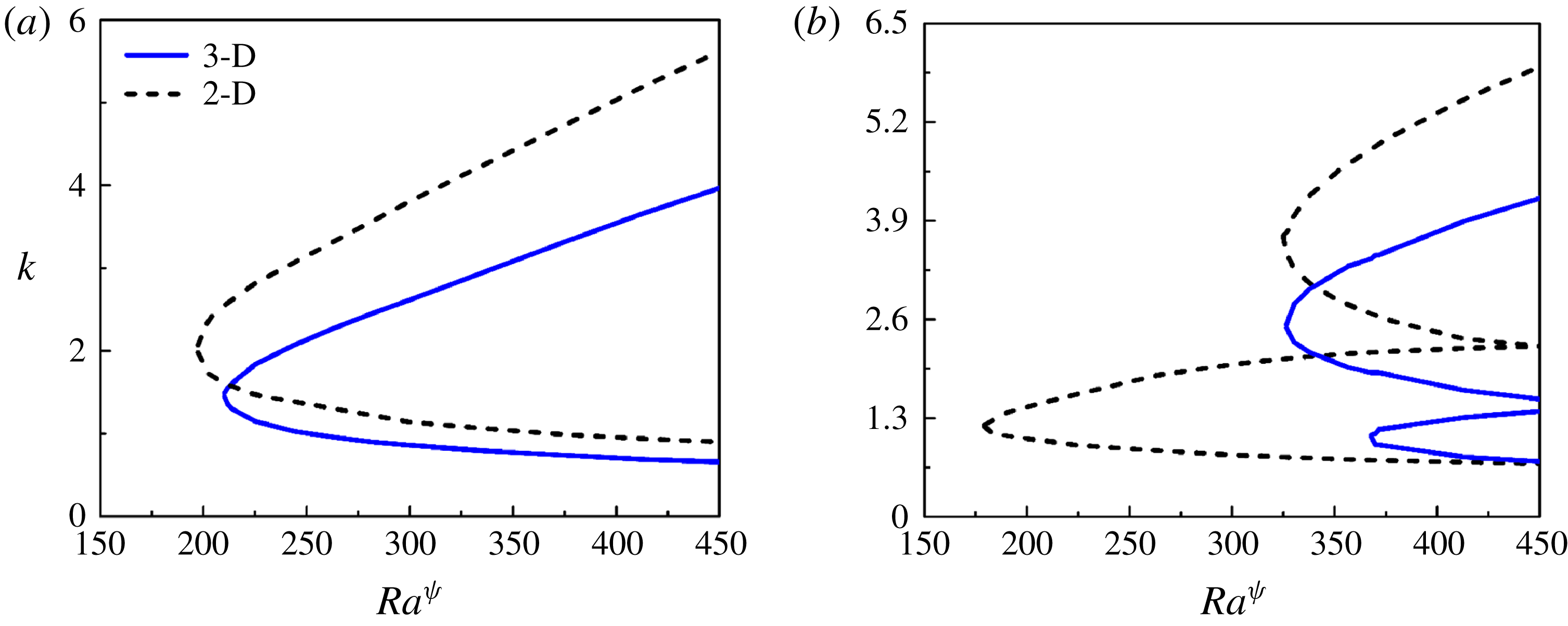
Figure 24. Neutral stability curves (a,b) show the variation of streamwise wavenumber (
 $k$
) with electric Rayleigh number (
$k$
) with electric Rayleigh number (
 $Ra^{\unicode[STIX]{x1D713}}$
) for two-dimensional (evenly broken line) and three-dimensional (solid line) perturbations. The other parameters for (a) are
$Ra^{\unicode[STIX]{x1D713}}$
) for two-dimensional (evenly broken line) and three-dimensional (solid line) perturbations. The other parameters for (a) are
 $V^{L}=1$
,
$V^{L}=1$
,
 $h=0$
,
$h=0$
,
 $\unicode[STIX]{x1D6FF}=0.02$
,
$\unicode[STIX]{x1D6FF}=0.02$
,
 $Sc=10$
and
$Sc=10$
and
 $Re=0.5$
. The other parameters for (b) are
$Re=0.5$
. The other parameters for (b) are
 $V^{L}=3$
,
$V^{L}=3$
,
 $h=-0.3$
,
$h=-0.3$
,
 $\unicode[STIX]{x1D6FF}=0.02$
,
$\unicode[STIX]{x1D6FF}=0.02$
,
 $Sc=10$
and
$Sc=10$
and
 $Re=0.5$
. The value of the spanwise wavenumber
$Re=0.5$
. The value of the spanwise wavenumber
 $m$
is set equal to
$m$
is set equal to
 $k$
for the three-dimensional cases.
$k$
for the three-dimensional cases.
Appendix C. Estimation of thickness of mixed layer
$\unicode[STIX]{x1D6FF}$

For the diffusion process, the length scale can be approximated as,
 $\unicode[STIX]{x1D6FF}\sim \sqrt{\unicode[STIX]{x1D705}t}$
. The diffusion coefficient
$\unicode[STIX]{x1D6FF}\sim \sqrt{\unicode[STIX]{x1D705}t}$
. The diffusion coefficient
 $\unicode[STIX]{x1D705}\sim O(10^{-9}-10^{-11})~\text{m}^{2}~\text{s}^{-1}$
(Petitjeans & Maxworthy Reference Petitjeans and Maxworthy1996; Lajeunesse et al.
Reference Lajeunesse, Martin, Rakotomalala, Salin and Yortsos1999), the time scale
$\unicode[STIX]{x1D705}\sim O(10^{-9}-10^{-11})~\text{m}^{2}~\text{s}^{-1}$
(Petitjeans & Maxworthy Reference Petitjeans and Maxworthy1996; Lajeunesse et al.
Reference Lajeunesse, Martin, Rakotomalala, Salin and Yortsos1999), the time scale
 $t$
can be approximated as,
$t$
can be approximated as,
 $t\sim O(10^{-1}-10^{-2})~\text{s}$
. Thus,
$t\sim O(10^{-1}-10^{-2})~\text{s}$
. Thus,
 $\unicode[STIX]{x1D6FF}$
is obtained as
$\unicode[STIX]{x1D6FF}$
is obtained as
 $\unicode[STIX]{x1D6FF}\sim O(10^{-5}-10^{-6})~\text{m}$
. This gives the dimensionless value of
$\unicode[STIX]{x1D6FF}\sim O(10^{-5}-10^{-6})~\text{m}$
. This gives the dimensionless value of
 $\unicode[STIX]{x1D6FF}\sim O(10^{-1}-10^{-2})$
considering the characteristic length to be
$\unicode[STIX]{x1D6FF}\sim O(10^{-1}-10^{-2})$
considering the characteristic length to be
 ${\sim}10^{-4}$
m. It was further confirmed through the nonlinear CFD simulations, the details of which are mentioned in § 3.5. Figure 25 shows the base-state scalar (
${\sim}10^{-4}$
m. It was further confirmed through the nonlinear CFD simulations, the details of which are mentioned in § 3.5. Figure 25 shows the base-state scalar (
 $S_{0}$
) profile, for
$S_{0}$
) profile, for
 $V^{L}=6$
. It can be seen from the figure that the thickness of the mixed interface at the base state is
$V^{L}=6$
. It can be seen from the figure that the thickness of the mixed interface at the base state is
 ${\sim}0.05$
.
${\sim}0.05$
.
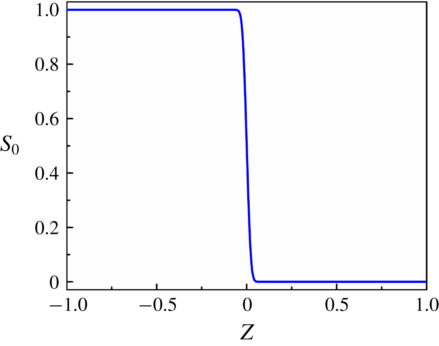
Figure 25. The variation of concentration scalar (
 $S_{0}$
) across the channel at the base state. The parameters considered for the simulation are
$S_{0}$
) across the channel at the base state. The parameters considered for the simulation are
 $h=0$
,
$h=0$
,
 $Sc=700$
and
$Sc=700$
and
 $V^{L}=6$
.
$V^{L}=6$
.