


1. Introduction
1.1. The broader context
Gas bubbles dispersed in a turbulent liquid flow control the transfer of mass and energy between phases in many environmental processes and industrial applications, such as wave breaking on the ocean surface (Deike, Melville & Popinet Reference Deike, Melville and Popinet2016; Deike, Lenain & Melville Reference Deike, Lenain and Melville2017) and bubble column reactors (Stöhr, Schanze & Khalili Reference Stöhr, Schanze and Khalili2009; Risso Reference Risso2018). Knowledge of how the turbulence impacts the quantity, size and dynamics of these bubbles is key to modelling their contributions to transfer rates (Deike & Melville Reference Deike and Melville2018). One simple yet still-open question regards the average speed at which the bubbles rise through the turbulent medium due to their buoyancy. Several analytical and experimental studies have characterized the rise of single bubbles in a quiescent medium, accounting for the effects of bubble size, liquid composition and the presence of impurities (Duineveld Reference Duineveld1995; Bel Fdhila & Duineveld Reference Bel Fdhila and Duineveld1996; Maxworthy et al. Reference Maxworthy, Gnann, Kürten and Durst1996; Mougin & Magnaudet Reference Mougin and Magnaudet2001; Park et al. Reference Park, Park, Lee and Lee2017), while the work on particle settling and rise rates in turbulence has shown non-trivial results (Nielsen Reference Nielsen1992).
1.2. Bubble rise in a quiescent medium
Before discussing the effects of turbulence, it is useful to summarize the dynamics of a bubble rising in a quiescent medium. The quiescent rise velocity  $v_{q}$ is given by a balance between the buoyant force lifting the bubble upwards and the stress from the oncoming flow opposing its motion, and is written as
 \begin{equation} v_{q} = \sqrt{4 d g / (3 C_{D})}, \end{equation}
where  $d$ is the bubble diameter,
  $g$ is the gravitational acceleration and
  $C_{D}$ is the drag coefficient. The drag coefficient is a function of the Reynolds number of the bubble's motion
  ${Re}_{q} = d v_{q} / \nu$ (where
  $\nu$ is the liquid kinematic viscosity), which represents the relative importance of inertial and viscous stresses, and the Bond number
  ${Bo} = \rho g d^2 / \sigma$ (where
  $\rho$ is the liquid density and
  $\sigma$ is the surface tension of the liquid–gas interface), which represents the relative importance of gravity and surface tension and should account for bubble deformability.
When the bubble is small and  ${Re}_{q} \ll 1$ and
  ${Bo} \ll 1$, the bubble remains spherical, and the drag is viscous. The drag coefficient is then well described with the relation for a solid sphere undergoing viscous drag,
  $C_{D} = 24 / {Re}_{q}$, leading to a quadratic relationship between the bubble diameter and the rise speed (Maxworthy et al. Reference Maxworthy, Gnann, Kürten and Durst1996).
Moderately sized air bubbles in water (up to  $d \approx 2$ to 3 mm) have
  ${Re}_{q} \gg 1$ and
  ${Bo} \leqslant 1$, for which the bubble shape is not significantly deformed, but the drag is inertial. Even larger bubbles, with
  ${Bo}>1$, become more deformed and adopt an oblate spheroidal shape, which increases the drag relative to a sphere of the same volume and causes the rise velocity to plateau near
  $30$ to
  $35\ \textrm {cm}\ \textrm {s}^{-1}$ (Duineveld Reference Duineveld1995; Mougin & Magnaudet Reference Mougin and Magnaudet2001). Bubble rise is modified when surfactants in the liquid adsorb to the bubble surface, which has been shown experimentally and numerically to reduce both deformation and the bubble rise velocity (Clift, Grace & Weber Reference Clift, Grace and Weber1978; Bel Fdhila & Duineveld Reference Bel Fdhila and Duineveld1996).
1.3. Particle motion in turbulence: the Maxey–Riley equation
When a particle rises or sinks by buoyancy forces through a carrier fluid in motion, it is submitted to additional forces. Here, we take a ‘particle’ to be a bubble, droplet or solid particle that has a different density than the liquid or gas surrounding it. We consider a particle of finite size that exerts no feedback onto the flow (as it may with the motion in its wake, for example) and neglect the Basset history force (which would result from its previous accelerations). Its motion is described by an equation of motion following the work of Maxey & Riley (Reference Maxey and Riley1983),
 \begin{equation} V_{p} \rho_{p} \dot{\boldsymbol{v}} = \boldsymbol{F}_{P} + \boldsymbol{F}_{M} + \boldsymbol{F}_{B} + \boldsymbol{F}_{L} + \boldsymbol{F}_{D}, \end{equation}
where  $V_{p}$ is the volume of the particle,
  $\rho _{p}$ is its density,
  $\boldsymbol {v}$ is its velocity and the terms on the right-hand side are, from left to right, the pressure force exerted on the particle, the added-mass force, the buoyancy force, the shear-induced lift force and the drag force.
The pressure force  $\boldsymbol {F}_{P}$, resulting from the pressure gradient in the carrier fluid, is expressed by invoking the Navier–Stokes equation for the carrier fluid velocity field
  $\boldsymbol {u}$, leading to
 \begin{equation} \boldsymbol{F}_{P} = \rho V_{p} \frac{\mathrm{D} \boldsymbol{u}}{\mathrm{D} t} = \rho V_{p} \left( \frac{\partial \boldsymbol{u}}{\partial t} + \boldsymbol{u} \boldsymbol{\cdot} \boldsymbol{\nabla} \boldsymbol{u} \right), \end{equation}
where  $\rho$ is the density of the carrier fluid. The added-mass force
  $\boldsymbol {F}_{M}$ arises from the fact that, as a particle accelerates, so must some surrounding fluid. It is given by
 \begin{equation} \boldsymbol{F}_{M} = C_{M} \rho V_{p} \left( \frac{\mathrm{D} \boldsymbol{u}}{\mathrm{D} t} - \dot{\boldsymbol{v}} \right), \end{equation}
where  $\boldsymbol {v}$ is the particle velocity and
  $C_{M}$ is the added-mass coefficient, equal to
  $0.5$ as determined experimentally for a solid sphere (Magnaudet & Eames Reference Magnaudet and Eames2000). The buoyancy force exerted on the particle is due to a density mismatch between the particle and the carrier fluid, given by
 \begin{equation} \boldsymbol{F}_{B} = (\rho - \rho_{p}) V_{p} g \boldsymbol{e}_z, \end{equation}
where  $g$ is the acceleration due to gravity and
  $\boldsymbol {e}_z$ is the direction opposite which gravity acts (upwards). The shear-induced lift force
  $\boldsymbol {F}_{L}$ arises when the bubble slips through a region of vortical flow, and is given by
 \begin{equation} \boldsymbol{F}_{L} ={-} C_{L} \rho V_{p} (\boldsymbol{v}-\boldsymbol{u}) \times (\boldsymbol{\nabla} \times \boldsymbol{u}), \end{equation}
where  $C_{L}$ is the lift coefficient. The lift coefficient is very sensitive to the flow conditions around the particle, and for deformable bubbles in shear flows, goes from positive to negative as bubbles exceed a certain size (Tomiyama et al. Reference Tomiyama, Tamai, Zun and Hosokawa2002; Salibindla et al. Reference Salibindla, Masuk, Tan and Ni2020). Finally, we model the drag exerted on the particle with
 \begin{equation} \boldsymbol{F}_{D} ={-} \frac{C_{D} \rho A_{p}}{2} | \boldsymbol{v} - \boldsymbol{u} | (\boldsymbol{v} - \boldsymbol{u}), \end{equation}
where  $A_{p}$ is the frontal area of a sphere with volume
  $V_{p}$ and
  $C_{D}$ is the drag coefficient, which is dependent on the condition at the particle surface and the Reynolds number
  ${Re}_{p} = \rho |\boldsymbol {v} - \boldsymbol {u}| d / \mu$, where
  $\mu$ is the carrier fluid viscosity, of the flow around the particle. For
  ${Re}_{p} \ll 1$, the drag on the particle is dominated by viscosity, and the drag coefficient is given by
  $C_{D} = 24/{Re}_{p}$, leading to a linear relationship between the slip velocity and drag force. When
  ${Re}_{p}$ is larger than 100, the drag force mainly originates from inertial forces. In this regime (but before the boundary layer around the sphere transitions to turbulence around
  ${O}({Re}_{p}) \approx 1\times 10^{5}$),
  $C_{D}=0.5$ is a good approximation for a rigid sphere, yielding a nonlinear relationship between the bubble slip velocity and the drag force. Note that recent work has investigated other nonlinear formulations of the drag for bubbles in quiescent flow (Barry & Parlange Reference Barry and Parlange2018).
For particles larger than the smallest scales of the flow, Faxén corrections can be employed to the above equations to filter the velocity field  $\boldsymbol {u}$ over the particle's scale (Calzavarini et al. Reference Calzavarini, Volk, Bourgoin, Lévêque, Pinton and Toschi2009; Homann & Bec Reference Homann and Bec2010). Finite size corrections to the Maxey–Riley equation are of primary importance to model accurately highly intermittent statistics such as particle accelerations. However, the large-scale statistics such as the velocity distribution should be much less sensitive to finite size corrections, which will be neglected in the present study.
When the carrier flow velocity field  $\boldsymbol {u}$ is turbulent, it is comprised of fluctuating motions over a range of scales, the smallest of which are characterized by the Kolmogorov scale
  $\eta$ (at which velocity fluctuations are quickly damped by viscous diffusion). The largest scale is usually defined as the integral length scale
  $L_{int}$, beyond which velocity fluctuations become uncorrelated (Pope Reference Pope2000). The scale of the fluctuations in the velocity is parameterized by
  $u'$, the root-mean-square of the velocity fluctuations.
1.4. Framing the problem: bubble rise in turbulence
To frame the problem in dimensionless terms, we first simplify the point-particle approximation for the case of light bubbles in a much denser fluid, considering the limit of negligible particle inertia,  $\rho _{p} \ll \rho$. Further, we take constant values for the added mass, drag and lift coefficients, neglecting their dependence on the local flow around the point bubble. We then non-dimensionalize (1.2) with two descriptors of the turbulent field
  $\boldsymbol {u}$: the integral length scale
  $L_{int}$ and the root mean square velocity fluctuation
  $u'$, writing
 \begin{equation} \tilde{x} = \frac{x}{L_{int}}, \quad \tilde{t} = \frac{t}{L_{int}/u'}, \quad \tilde{\boldsymbol{v}} = \frac{\boldsymbol{v}}{u'}, \quad \tilde{\boldsymbol{u}} = \frac{\boldsymbol{u}}{u'}, \end{equation}
so that (1.2) reads
 \begin{align} \frac{4 d^* C_{M}}{3 C_{D}} \dot{\tilde{\boldsymbol{v}}} = \frac{4 d^* (1+C_{M})}{3 C_{D}} \frac{\mathrm{D} \tilde{\boldsymbol{u}}}{\mathrm{D} \tilde{t}} + \frac{1}{{\beta}^2} \boldsymbol{e}_z - \frac{4 d^* C_{L}}{3 C_{D}} (\tilde{\boldsymbol{v}}-\tilde{\boldsymbol{u}}) \times (\tilde{\boldsymbol{\nabla}} \times \tilde{\boldsymbol{u}}) - | \tilde{\boldsymbol{v}} - \tilde{\boldsymbol{u}} | (\tilde{\boldsymbol{v}} - \tilde{\boldsymbol{u}}) . \end{align}
For simplicity, we refer to the first term on the right-hand side, which is a combination of the pressure and added-mass terms, as the pressure term.
This equation defines the dimensionless turbulence intensity  $\beta =u'/v_{q}$ and the dimensionless bubble size
  $d^*=d/L_{int}$. The drag coefficient is a function of the bubble inertia and deformability, and is usually parameterized as a function of the bubble's Bond number
  ${Bo} = \rho gd^2 / \sigma$ and its quiescent Reynolds number
  ${Re}_{q} =d v_{q}/\nu$, while one might also consider the drag and lift coefficients to depend on the local turbulence characteristics. The turbulence can be characterized by the large-scale turbulence Reynolds number
  ${Re}_{t} = L_{int} u' / \nu$.
In total, the problem involves 8 dimensional variables ( $\left \langle v_z \right \rangle$,
  $d$,
$d$,  $g$,
$g$,  $\sigma$,
  $\rho$,
  $L_{int}$,
  $\nu$ and
  $u'$), together spanning three dimensions. Invoking Buckingham's
  $\varPi$ theorem, we then have five dimensionless variables, leading us to look for the average dimensionless rise velocity
  $\left \langle v_z \right \rangle /v_{q}(d,g,\sigma /\rho )$ as a function of the four independent dimensionless parameters
 \begin{equation} \beta = \frac{u'}{v_{q}(d,g,\sigma/\rho)}, \quad {Bo} = \frac{g d^2}{\sigma/\rho}, \quad d^* = \frac{d}{L_{int}}, \quad \textrm{and} \quad {Re}_{t} = \frac{L_{int} u'}{\nu}, \end{equation}
where  $v_{q}$ is the quiescent rise velocity, set by the other variables.
Other relevant dimensionless parameters can be defined as a function of the four that we have chosen. The turbulent Weber number,  ${We}$, gives the ratio between the turbulent stresses acting on a bubble, which deform it, and the restoring force of surface tension, which works to maintain a spherical shape. With
  $v_{q}$ defined as
  $v_{q} = \sqrt {4 dg / (3 C_{{D}})}$ and
  $d$ within the inertial subrange of the turbulence, the turbulent Weber number can be written as
  ${We} = \epsilon ^{2/3} d ^{5/3} / (\sigma /\rho ) = (0.7 u'^3/L_{int})^{2/3} d ^{5/3} / (\sigma /\rho ) = 0.79 (4 / 3C_{D}) \beta ^2 {Bo} \,d^{*2/3}$. The quiescent particle Reynolds number,
  ${Re}_{q} = \rho v_{q} d / \mu$, gives the ratio between the inertial and viscous forces acting on the bubble as it rises in a quiescent flow, and (as will become evident) for small
  $\beta$ gives the approximate scale of the instantaneous particle Reynolds number
  ${Re}_{p} = \rho |\boldsymbol {v}-\boldsymbol {u}| d / \mu$. Note that
  ${Re}_{q} = {Re}_{t} d^* /\beta$. Finally, the bubble Froude number,
 \begin{equation} {Fr} = \frac{u'}{\sqrt{dg}}, \end{equation}
is a parameterization of the turbulence intensity, but unlike  $\beta$, is agnostic to the quiescent drag coefficient
  $C_{{D}}$. It can be expressed by removing the drag coefficient dependence of
  $\beta$ with
  ${Fr} = \beta \sqrt {3 C_{{D}}/4}$.
In this study, we will focus on the effects of  $\beta$ and
  $d^*$, neglecting the impact of bubble deformation and assuming that
  ${Re}_{q}$ is large enough to yield a constant drag coefficient.
1.5. Heavy particles in turbulence
Here, we briefly review work on the related problem of the settling speeds of heavy particles in turbulence. Wang & Maxey (Reference Wang and Maxey1993) showed through simulations of particles subject to Stokes drag, which is proportional to the slip velocity, that such particles tend to settle faster in the presence of turbulence than in an otherwise stationary flow. This occurs to the greatest extent when the particle's response time  $\tau _{p} = \rho _{p} d^2 / 18 \mu$ (which sets the quiescent settling velocity as
  $v_{q} = \tau _{p} g$) is comparable to the Kolmogorov time scale of the turbulence,
  $\tau _\eta$, which is the time scale of the smallest turbulent motions. Shorter particle response times allow the particle to immediately adapt to the changing surroundings, while longer particle response times filter out some of the turbulent motions. The increase in settling rate has been attributed to the particles' inertia causing them to spiral out of regions of rotating flow and accumulate on the ‘fast tracks’ of fast-moving downwards flow between eddies (Maxey & Corrsin Reference Maxey and Corrsin1986).
While the above results suggest that viscous drag leads to a Kolmogorov scaling and increased settling rates, a different picture emerges when  ${Re}_{p}$ is larger and the heavy particle experiences nonlinear drag. This nonlinearity means that slip in the horizontal directions increases the drag force in the vertical direction, slowing the settling of heavy particles or rise of light particles. Fornari et al. (Reference Fornari, Picano, Sardina and Brandt2016) simulated the settling of many large spherical particles in turbulence (with
  $d \approx 12 \eta$), and Byron et al. (Reference Byron, Tao, Houghton and Variano2019) performed experiments measuring the velocity of single non-spherical particles in the inertial subrange settling in turbulence. In these scenarios, finite-size effects filter out turbulent motions which are smaller than the particle. Both studies found that the turbulence reduced the settling rate. For the simulations, this was attributed to the increase in the vertical inertial drag due to horizontal slip (Fornari et al. Reference Fornari, Picano, Sardina and Brandt2016). In the experiments, a strong correlation between the average settling rate and the average slip velocity was found, with a vertical offset representing the average settling speed (Byron Reference Byron2015).
1.6. Light particles and bubbles in turbulence
In this section, we summarize previous work characterizing the rise of bubbles and buoyant particles in turbulence. Figure 1 shows the parameter space of conditions explored through various experimental and numerical studies, in terms of the non-dimensional parameters introduced in § 1.4. In panel (a), the horizontal axis shows the logarithmic position of the bubble's diameter  $d$ in relation to the Kolmogorov and integral length scales of the turbulence,
  $\eta$ and
  $L_{int}$, and the vertical axis shows
  $\beta$, the ratio between the fluctuation velocity of the turbulence
  $u'$ and the bubble's quiescent rise speed
  $v_{q}$. In panel (b), the horizontal axis shows the quiescent Reynolds number
  ${Re}_{q}$, which will serve as a lower bound for the typical value of the Reynolds number describing the instantaneous flow around the bubble, and the vertical axis shows the turbulent Weber number
  ${We} = \epsilon ^{2/3} d^{5/3} \rho / \sigma$, which represents the extent to which the bubble is deformed by the background turbulence in the liquid. In the limit of a large density and viscosity ratios (for example, considering air bubbles in water), the use of
  $\beta$, We,
  $Re_q$ and
  $d^{*}$ (in place of
 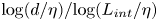 ${\rm log}({d}/\eta)/{\rm log}({L}_{int}/\eta)$) fully describes the problem of bubble rise in homogeneous, isotropic turbulence.

Figure 1. The range of parameters considered in this paper and comparable experiments (black, filled markers), direct numerical simulations (green, open makers) and point-bubble simulations (blue, point-like markers). (a) The turbulence intensity and dimensionless bubble sizes. The horizontal axis places the bubble diameter  $d$ in relation to the turbulent scales
  $\eta$ and
  $L_{int}$, and the vertical axis shows the velocity scale of the turbulent fluctuations normalized by the bubble's quiescent rise velocity. The joint distribution of these quantities for our experimental measurements is shaded in the background. The dash-dotted line corresponds to the main series of point-bubble simulations we present. (b) The turbulent deformation Weber number We and the bubble quiescent Reynolds number
  $Re_q$, for experiments, direct numerical simulations and point-bubble simulations. Most studies were performed in the range
  ${We}<1$ and
  ${Re}_{q}>10$, for which the bubble deformation is of small amplitude, and the drag force starts to be nonlinear in the slip velocity.
Aliseda & Lasheras (Reference Aliseda and Lasheras2011) studied the motion of  $10$ to
  $900\ \mathrm {\mu }\textrm {m}$ air bubbles (comparable to the Kolmogorov microscale
  $\eta$) in a turbulent water flow with low void fraction (
 ${<}10^{-3}$) and found that the turbulence decreased the bubbles’ rise velocity. Comparing the measured rise velocities with the velocity predicted with a quiescent background and a contaminated interface, a maximum reduction in rise velocity occurred when the bubble's viscous response time equals the Kolmogorov time scale. Taken alongside results for heavy particles from Wang & Maxey (Reference Wang and Maxey1993), this points to a mechanism that suggests that turbulent motions have the greatest impact on particles comparable to the Kolmogorov scales when the drag on the particles is viscous. Similarly, Poorte & Biesheuvel (Reference Poorte and Biesheuvel2002) found a decrease in rise velocity of up to 35 % for bubbles close to the smallest scales of the turbulence in weak turbulence, with
  $\beta < 0.5$. Their data presented reasonable agreement with a turbulent scale-dependent model from Spelt & Biesheuvel (Reference Spelt and Biesheuvel1997) for lower values of
  $\beta$ and linear (viscous) drag.
Turning to the behaviour of bubbles with larger sizes (closer to the integral scale of the turbulence), one may expect that large-scale turbulent motions, now comparable to the bubble size, are less effective at advecting the bubble through the water. Prakash et al. (Reference Prakash, Tagawa, Calzavarini, Mercado, Toschi, Lohse and Sun2012) measured the rise velocities of  $d\approx {3}\ \textrm {mm}$ bubbles, with
  $d\approx 10 \eta$, in a vertical water flow with low
  $\beta$, finding a
  ${\sim } 20\,\%$ reduction relative to their quiescent rise rate, which slightly increased in magnitude with increasing turbulence. Kawanisi, Nielsen & Zeng (Reference Kawanisi, Nielsen and Zeng1999) showed with experiments of light particles in grid-generated turbulence and point-bubble simulations in a turbulent-like velocity field that increasing turbulence intensity (with
  $\beta$ between
  ${\sim }1$ and
  ${\sim }10$) decreases the mean rise rate.
Direct numerical simulation (DNS) of bubbles in turbulence remains limited. The rise through turbulence of a deformable bubble of the size of the Taylor microscale,  $d = \lambda \approx 10 \eta \approx L_{int}/2$, was studied with DNS (with the level-set method and surface tension) by Loisy & Naso (Reference Loisy and Naso2017) with
  ${Re}_\lambda =\lambda u' / \nu = 30$. With the turbulence parameters and bubble size held constant, the gravitational acceleration was changed in order to study the effect of the ratio of the bubble's quiescent rise rate to the velocity scale of the turbulence, yielding
  $\beta = 0.5$, 0.9 and 1.6. Turbulence reduced the rise velocity to the greatest extent when
  $\beta \approx 1$. Reichardt, Tryggvason & Sommerfeld (Reference Reichardt, Tryggvason and Sommerfeld2017) carried out DNS (using pseudo-spectral forcing with a finite difference/front-tracking method) of large bubbles in much weaker turbulence, with
  $\beta < 0.1$, and found that less-deformable bubbles are slowed to a greater extent than more-deformable ones (note that this study was performed at
  ${Re}_{\lambda } < 10$).
Simulations of infinitesimally small bubbles immersed in an uncoupled velocity field have also contributed to our understanding of bubble rise dynamics in turbulence. With a linear drag force, Mazzitelli & Lohse (Reference Mazzitelli and Lohse2004) showed a maximum reduction in rise velocity when the bubble's response time is equal to the Kolmogorov time scale. Snyder et al. (Reference Snyder, Knio, Katz and Le Maître2007) carried out simulations of point bubbles using a drag force dependent on the bubble's instantaneous local Reynolds number, yielding linear drag (with respect to the slip velocity) for  ${Re}_{p}<1$ and nonlinear drag at higher Reynolds numbers, and found a decrease in bubble rise velocity at all conditions. Inclusion of the lift force was shown to only slightly reduce the mean rise speed beyond the value obtained with no lift force. As in the data from Poorte & Biesheuvel (Reference Poorte and Biesheuvel2002), the skewness of the bubble vertical velocity probability density function obtained from the point-bubble simulations from Snyder et al. (Reference Snyder, Knio, Katz and Le Maître2007) are dependent on both the non-dimensional turbulence intensity
  $\beta$ and the ratio between the bubble size and the turbulent length scales.
Finally, we note two studies that found an increase in rise speed in turbulence. Salibindla et al. (Reference Salibindla, Masuk, Tan and Ni2020) present experiments in which the velocity field around bubbles was measured with tracer particles and showed that, with a fixed intensity of the turbulence, bubbles below a certain size over-sample regions of  $u_z < 0$, while larger bubbles over-sample
  ${u_z > 0}$, leading to an increase in rise speed. The size at which the switch occurs is attributed to the increased deformation of the bubble and the lift coefficient
  $C_{L}$ becoming negative. Additionally, Friedman & Katz (Reference Friedman and Katz2002) found that small diesel fuel droplets, which are slightly less dense than water, had their rise speeds increased by turbulence to six times greater than the quiescent rate. This increase is explained by the ‘fast-tracking’ phenomena discussed by Maxey & Corrsin (Reference Maxey and Corrsin1986) in which sufficiently heavy particles are expelled to the outsides of rotational flow structures, where the velocity is the greatest, and follow the ‘fast tracks’ between the eddies (Nielsen Reference Nielsen2007).
1.7. Paper outline
While the majority of experiments have shown a decrease in bubble rise speed due to turbulence, the sometimes contradictory results and interpretation in the literature and the complexity of the phenomena for both light and heavy particles moving in turbulence motivate this work.
This paper presents an experimental and numerical study on the rise velocity of bubbles in turbulence. We focus on the direct effect of two non-dimensional numbers on the rise speed in turbulence: the effective bubble size  $d^* = d/L_{int}$ and the turbulence intensity
  $\beta = u'/v_{q}$ (or, at times, the Froude number
  ${\textit {Fr}} = u'/\sqrt {gd}$). The effect of the bubble deformability is not studied directly but is implicit due to its effect on the rise velocity at low turbulence.
In § 2, we describe the turbulence generation and bubble tracking methods employed in the experiment. Section 3 presents the experimental results, which reveal that the average rise speed of a bubble is slowed to a greater extent in stronger turbulence. In § 4, we introduce the point-bubble simulations employing the Maxey–Riley equation, employ results to extract the mechanisms by which turbulence slows a bubble down, and compare the simulation and experimental results. Section 5 presents a simple theoretical model to describe the regimes of the slowdown in the limits of small and large Froude number (or  $\beta$, as the two parameters differ only according to the quiescent drag coefficient). Finally, in § 6, we compare our results to those from other studies on bubbles rising through turbulence, and discuss additional effects not considered in our analysis, such as bubble deformability, finite-size filtering effects and the structure of the large-scale mean flow.
2. Experimental methods
2.1. Turbulence generation and bubble injection
The experiment consists of a  ${0.37}\ \textrm {m}^{3}$ tank filled with deionized water, as sketched in figure 2(a). Turbulence in the water is generated by four submerged water pumps (Eco-Worthy 1100 GPH 12 V Bilge Pumps), the flow from each of which is split at a T into two parallel jets. Each of the four sets of parallel jets is positioned at the corner of a horizontal 25 cm square, and the convergence of the jets creates a turbulent region at the centre of the square. Compared with other turbulence-generation systems that use comparable submerged pumps (Variano & Cowen Reference Variano and Cowen2008; Byron et al. Reference Byron, Tao, Houghton and Variano2019), ours is constructed at a much smaller scale, giving the on/off state of any pump much greater influence on the immediate state of the flow in the turbulent zone. Therefore, instead of employing a randomly generated pattern with which to activate each pump, we run each pump continuously.

Figure 2. (a) A schematic of the experiment, showing the air injection needle and representative bubble trajectory, pumps submerged in a water tank to create turbulence, a laser and high-speed camera for particle image velocimetry and two cameras for three-dimensional bubble tracking. (b) A bubble trajectory (blue) and the region of strong turbulent fluctuations in one of the nine particle image velocimetry planes (red).
The resulting flow field consists of a region of intense turbulence where the jets meet. Below that region, there is decreasing turbulence and a significant downwards flow (out of the converging zone), comparable in magnitude to the bubbles’ rise velocity. In our experiment, we take advantage of this heterogeneity to probe a range of turbulent conditions in a single experiment, as the turbulent fluctuations and length scales change considerably.
Bubbles are injected through a needle fed by a pressurized air line at the bottom of the tank, with the injection rate controlled by a flow controller (Alicat). The injection rate is slow enough to enable the tracking of bubbles optically, and the void fraction ( ${\ll }0.1\,\%$) is sufficiently low that we expect no feedback onto the turbulence from the bubbles (Rensen, Luther & Lohse Reference Rensen, Luther and Lohse2005). The typical distance between a bubble and its closest neighbour is approximately 5 cm, above 10 times the typical bubble diameter. Our tank is left open to the atmosphere, and it will become contaminated with surfactants (typically reaching a steady state in contamination after half an hour), which will adsorb to the bubble interfaces (Van Dorn Reference Van Dorn1966; Clift et al. Reference Clift, Grace and Weber1978; Henderson & Miles Reference Henderson and Miles1990; Deike, Berhanu & Falcon Reference Deike, Berhanu and Falcon2012).
To confirm that the results are not merely a result of the turbulence generation method, a second set of experiments was carried out in a similar, smaller tank involving pump-generated turbulence with a different spatial arrangement of pumps, and similar turbulence characterization and bubble tracking methods. This set-up is described in Appendix B, and the main results reported in this paper are shown using data from both experiments.
2.2. Turbulence characterization with particle image velocimetry
The turbulent flow field is characterized with two-dimensional, two-component particle image velocimetry (PIV) (Thielicke & Stamhuis Reference Thielicke and Stamhuis2014) performed in 9 parallel planes, each separated by approximately 2 cm. The water is seeded with  ${25}\ {\mathrm {\mu }}\textrm {m}$ polyamide 12 particles with a seeding density of approximately
  ${30}\ \textrm {g}\ \textrm {m}^{-3}$. The imaged plane is illuminated with a sheet of 532 nm light generated with a 2 W laser and optics and imaged with a high-speed camera (Phantom VEO4K-PL) equipped with a 100 mm lens. The duration between the two frames used to calculate each velocity field is 1/1400 s, and the duration between each velocity field is 1/100 s. For each plane, approximately 3 min of data are obtained. The location of the front and back planes and qualitative turbulence intensity results from an interior plane are shown relative to a bubble trajectory in figure 2(b).
2.2.1. Calibration
To calibrate the PIV set-up, a planar calibration target (created by laser engraving a pattern on an acrylic sheet) is brought into focus by traversing it along a positioning arm aligned with the camera's axis, which defines the  $y$ axis of the coordinate system. The rows and columns of dots on the calibration plate correspond to the
  $x$ and
  $z$ (vertical) directions of the coordinate system, respectively. Pixels in the recorded images are mapped to
  $(x,z)$ positions using a perspective transformation in the Python implementation of OpenCV (Bradski Reference Bradski2000).
2.2.2. Flow-field and turbulent velocity-scale calculation
For each PIV plane positioned at  $y=y_{j}$, the horizontal and vertical components of the water velocity
  $u_x(x,y_{j},z,t)$ and
  $u_z(x,y_{j},z,t)$ are computed using
  ${32}\ \textrm {pix} \times {32}\ \textrm {pix}$ windows with 50 % overlap between adjacent windows, resulting in approximately 1.8 mm between velocity vectors. The mean flow
  $(\overline {u_x}(x,y_{j},z),\overline {u_z}(x,y_{j},z))$ is calculated by averaging each in time. The turbulent fluctuations
  $\widehat {u_x}(x,y_{j},z,t)$ and
  $\widehat {u_z}(x,y_{j},z,t)$ are calculated by subtracting the mean flow from the velocity field, and the root-mean-square fluctuations are calculated with
 \begin{equation} \left.\begin{gathered} u'_x(x,y_{j},z) = \sqrt{ \overline{\widehat{u_x}(x,y_{j},z,t)^2}} = \sqrt{ \overline{\left(u_x(x,y_j,z,t) - \overline{u_x}(x,y_{j},z) \right)^2}}, \\ u'_z(x,y_{j},z) = \sqrt{ \overline{\widehat{u_z}(x,y_{j},z,t)^2}} = \sqrt{ \overline{\left(u_z(x,y_j,z,t) - \overline{u_z}(x,y_{j},z) \right)^2}}. \end{gathered}\right\} \end{equation}
 The mean flow-field and turbulent fluctuations for three of the nine planes are shown in figure 3. The flow is not completely isotropic, as the centrelines of the jets used to create the turbulence all lie in the  $x$–
$x$– $y$ plane. This leads to stronger fluctuations measured in the
  $x$ direction than the
  $z$ direction: typically,
  $u'_x > u'_z$. We approximate the turbulence root-mean-square fluctuation velocity as
  $u'=\sqrt {({u_x'}^2 + {u_z'}^2)/2}$.

Figure 3. Summary of PIV results. (a) From left to right, the mean flow, the fluctuations in the  $x$ and
  $z$ directions, and integral length scale in three of the nine PIV planes. (b) The location of the nine PIV planes in the tank. The three coloured ones correspond to the three for which fields are shown above. (c) The integral of the autocorrelation function from which the integral length scale is calculated, at the three points marked by x markers in each field. (d) The structure function at the three marked points. (e) The compensated structure function at the corresponding points. The dashed lines give estimates of the dissipation rate with
  $0.7 u'^3/L_{int}$.
Additionally, we calculate the longitudinal structure function  $D_{LL}(\Delta r)$ at each point in the PIV plane with
 \begin{align} D_{{LL}}(x,y_{j},z,\Delta r) &= \frac{1}{4} \sum_{i={-}1,+1} \left( \overline{ \left(\widehat{u_x}(x+i\Delta r,y_{j},z,t) - \widehat{u_x}(x,y_{j},z,t)\right)^2 } \right. \nonumber\\ &\quad +\left. \overline{\left(\widehat{u_z}(x,y_{j},z+i\Delta r,t) - \widehat{u_z}(x,y_{j},z,t)\right)^2 } \right), \end{align}
which is shown for a point (marked with an x in the fields in (a)) in three of the PIV planes in figure 3(d). This structure function can be used to calculate the typical turbulent stress at the bubble scale,  $\rho D_{LL}(d)/2$. Since each PIV window overlaps with its neighbours by 50 %, our calculation of
  $D_{LL}(\Delta r)$ will underestimate the true value for values of
  $\Delta r$ close to the PIV window size, which is approximately 3.7 mm.
Additionally, we estimate the local turbulent dissipation rate using the relation  $\epsilon = {0.7} u'^3 / L_{int}$, where
  $L_{int}$ is the integral length scale of the turbulence (Sreenivasan Reference Sreenivasan1998). This agrees reasonably well with the relation
  $D_{LL}(\Delta r) = C_2(\epsilon \Delta r)^{2/3}$, with the Kolmogorov constant
  $C_2 = 2.0$, evaluated by considering the compensated structure function
  $(D_{LL}/C_2)^{3/2} / \Delta r$ (Pope Reference Pope2000). Figure 3(e) compares these two methods of determining
  $\epsilon$ at three separate points in the flow field.
Our flow is heterogeneous by nature, due to the regions of high turbulent intensity within the jets and the recirculation patterns that arise around it. As the injected power is constant over the experiments and the experiments are carried out over a long time, it is eventually balanced by dissipation and the turbulent flow is stationary. The spatial heterogeneity allows us to probe a range of turbulent conditions in a single experiment. In Appendix A, we show that in the Lagrangian sense as seen by the bubbles,  $u'$ typically changes over a scale not much shorter than the integral time scale of the turbulence. We nevertheless use the standard structure function and relationships used for homogeneous and isotropic turbulence to characterize the intensity and length scale of the flow. Additionally, we show that the velocity gradients of the mean flow are not responsible for the reduction in rise velocity we report. Finally, as the void fraction of bubbles in the turbulence region is negligible, we neglect the bubble feedback onto the turbulent statistics.
2.2.3. Turbulent length scales
Around each measure point of a PIV plane, the integral length scale is computed using the longitudinal autocorrelation function of the velocity fluctuations in the vertical and horizontal directions,
 \begin{align} \rho_{11}(x,y_j,z,\Delta r) &= \frac{1}{4} \sum_{i={-}1,+1} \left( \frac{\overline{ \widehat{u_{x}}(x,y_{j},z,t) \widehat{u_{x}}(x+i\Delta r,y_{j},z,t)}}{{u'}_x(x,y_j,z)^2} \right. \nonumber\\ &\quad + \left. \frac{\overline{ \widehat{u_{z}}(x,y_{j},z,t) \widehat{u_{z}}(x,y_{j},z+i\Delta r,t)}}{{u'}_z(x,y_j,z)^2} \right). \end{align}
As with the longitudinal structure function (2.2), fewer directions are considered for points near the PIV field boundaries. The integral length scale at a point in the flow is estimated with
 \begin{equation} L_{int}(x,y_{j},z) = \max \left( \int_0^{\Delta r_{max}} \rho_{11}(x,y_{j},z,\Delta r) \,\textrm{d} \Delta r \right), \end{equation}
which involves the maximum value of the integral instead of its value at  $\Delta r_{max}$ since the correlation functions are not completely converged for large distance separation. The fields of
  $L_{int}$ for three of the nine PIV planes, and the integral in (2.4) for one point in each plane, are shown in figure 3.
The dissipation rate is estimated as  $\epsilon (x,y_{j},z) = 0.7 u'^3/L_{int}$ (Sreenivasan Reference Sreenivasan1998), which under the isotropic assumption enables the estimation of the Taylor microscale with
 \begin{equation} \lambda = \sqrt{15\frac{\nu}{\epsilon}}u', \end{equation}
and the Kolmogorov microscale with  $\eta = (\nu ^3 / \epsilon )^{1/4}$.
The turbulence length scales, like the other quantities, vary spatially in the experiments due to the heterogenous nature of the flow. The range of values they take is included in the summary of turbulent conditions given in § 2.2.5. We remind the reader that those have been computed using relationships derived for homogeneous and isotropic turbulent flow, while our flow presents inhomogeneous features, so that they should be considered only as estimates of the turbulence length scales.
Note that we have computed the autocorrelation function to verify the absence of characteristic length scales above the integral length scale. The autocorrelation functions in the various PIV planes decay exponentially above the estimated  $L_{int}$ value, which validates the absence of any significant larger characteristic length scales in the flow fluctuations.
2.2.4. Three-dimensional interpolation of PIV results
The flow characteristics are first computed individually for each PIV plane. Once this is done, the computed quantities–the mean flow, the root-mean-square (r.m.s.) fluctuations and the integral length scale–are interpolated onto a grid of common  $(x,z)$ locations, with each plane differing in its
  $y$ position.
The interpolated results from all the planes are stacked in the  $y$ direction, forming a three-dimensional grid of data. This allows for the three-dimensional interpolation of any computed quantity given an
  $(x,y,z)$ bubble location. The Taylor microscale
  $\lambda$, Kolmogorov microscale
  $\eta$, and dissipation rate
  $\epsilon$ are calculated using the interpolated values of the measured quantities.
2.2.5. Summary of turbulent conditions
Table 1 summarizes the turbulent conditions generated in our experiment. Since the experiment is by design inhomogeneous, we present the 10th, 50th and 90th percentiles of the quantities as sampled by the bubbles, which is determined by the process we describe in the next section.
Table 1. Distribution of turbulent conditions probed by the bubbles. The 10th, 50th and 90th percentiles of each quantity are given.

2.3. Bubble triangulation and tracking
Bubbles are filmed with two synchronized cameras (Basler acA1440-220um) outfitted with 16 mm lenses, each recording at 200 Hz, as sketched in figure 2. The experiment is back lit with two spot lights shining on translucent paper behind the experiment. For each view, the background is determined by taking the 90th percentile of pixel intensities over whole movie at each pixel location. The background is subtracted from each image, images are binarized using a pixel intensity threshold, the bright regions inside the bubbles are filled in and the projected area (in number of pixels) and image location of each bubble is stored.
2.3.1. Three-dimensional triangulation
The traversing calibration plate is used to map each pixel in each camera to the light ray in three-dimensional space that reaches the pixel (Machicoane et al. Reference Machicoane, Aliseda, Volk and Bourgoin2019). Then, for each pair of images taken at a given point in time, three-dimensional bubble locations are determined by finding the near-intersection of rays through each of the bubbles identified in each camera's view. Since each calculated ray passes through the centroid of the bubble image as projected into the individual camera, and the bubbles are not spherical, the two rays corresponding to one bubble are not expected to exactly intersect in space. To allow for this and small errors in the calibration procedure, we allow for a maximum distance of up to 1 mm between corresponding rays, but this triangulation error is typically much closer to 0.2 mm.
Bubbles are triangulated in three-dimensional space with a process that minimizes the number of unpaired bubbles, the triangulation error and the discrepancy in physical size of each bubble as determined from each camera's view. The pixel size is calculated locally for each triangulated bubble, since the image magnification varies with distance from the camera. The bubble diameter  $d$ is determined with the average equivalent diameter of the bubble in the two views, given the projected area into each camera. Python code implementing the method is available at https://github.com/DeikeLab/stereo-triangulation.
2.3.2. Bubble tracking
Once the three-dimensional positions of bubbles are determined for each point in time, trajectories are constructed using the open-source Python package Trackpy (Allan et al. Reference Allan, Caswell, Keim and van der Wel2019), with each bubble allowed a maximum speed of  ${2}\ \textrm {m}\ \textrm {s}^{-1}$. To avoid considering spurious trajectories, we consider only trajectories lasting at least 0.025 s, although most trajectories are much longer. Since we do not report quantities such as a single bubble's mean velocity or its velocity's autocorrelation, our results are insensitive to instances in which a single bubble's trajectory is split into multiple separate trajectories.
Each bubble's absolute velocity  $\boldsymbol {w}(t)$ is calculated by differentiating its position
  $\boldsymbol {x}_{b}(t)$ with respect to time using a central difference scheme. To account for the variations in bubble shape that affect the measured bubble size, each bubble's diameter
  $d$ is taken to be the median of all the instantaneous
  $d$ values from its trajectory.
3. Experimental results
Our experimental dataset consists of three-dimensional bubble trajectories obtained by injecting air through needles of various sizes. Multiple bubbles are often observed in the experiment simultaneously, and in total, we have approximately  $4.25\times 10^{5}$ observations of bubble velocities, for which we also know the bubble size and local statistics of the turbulence in the absence of bubbles. With the bubbles tracked at
  $1/\Delta t = {200}\ \textrm {Hz}$, this corresponds to approximately
  $35\ \textrm {bubble}-\textrm {minutes}$ of experimental data. With the observation times normalized by the local integral time scale of the turbulence, and each integral time scale constituting one roughly independent event, we have an estimate of
 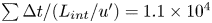 $\sum \Delta t/(L_{int}/u') = 1.1\times 10^{4}$ independent events in the entire dataset.
3.1. Phenomenological description of three-dimensional displacement of bubble rise through turbulence
To validate the correspondence between the bubble velocities and the water velocity field data, we note that with no horizontal buoyant force exerted on the bubbles, we expect the mean value of the horizontal velocities of bubbles passing through any point to be equal to the mean horizontal velocity of the water at that point. To this end, we compute the joint distribution of the bubble horizontal velocity  $w_x(t)$ and the water mean velocity at the bubble locations
  $\overline {u_x}(\boldsymbol {x}_{b}(t))$ for all the bubble trajectories, which is shown in figure 4(a). The mean horizontal velocities of bubbles passing through regions with each value of
  $\overline {u_x}(\boldsymbol {x}_{b}(t))$ is shown as the solid red line. Since this line falls on the dashed blue line representing
 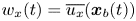 $w_x(t) = \overline {u_x}(\boldsymbol {x}_{b}(t))$, we are confident that the PIV data capture the mean water flow experienced by the bubbles.

Figure 4. In black and white, the joint distributions of bubble and mean water velocities in the horizontal (a) and vertical (b) directions. Darker regions correspond to a greater number of measurements. The solid line represents the mean velocities of bubbles when they are at a point in the flow with a given mean water velocity. The correspondence between the mean value of  $w_x$ and the local value of
  $\bar {u}_x(\boldsymbol {x}_b)$ shown in (a) suggests the mean bubble horizontal motion aligns with the mean water horizontal motion. The offset between the mean value of
  $w_z$ and the local value of
  $\bar {u}_z(\boldsymbol {x}_b)$ shown in (b) suggests that the bubbles typically have a positive vertical velocity relative to the surrounding mean flow.
Similarly, the plot in figure 4(b) compares the vertical velocities of the bubbles  $w_z(t)$ to the mean vertical velocity of the water
  $\overline {u_z}(\boldsymbol {x}_{b}(t))$ at the bubbles’ instantaneous locations. First, we note that bubbles are observed much more often in regions of mean downwards water flow,
 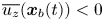 $\overline {u_z}(\boldsymbol {x}_{b}(t))<0$. This results from the fact that, in the laboratory frame of reference, bubbles linger in regions where the local downwards water velocity is approximately opposite to their slip velocity, which is typically upwards. This effect is accounted for in our analysis through the subtraction of the local mean water velocity from the observed bubble velocities. Secondly, we see that the mean value of a bubble's vertical velocity is greater than the local value of the mean vertical water velocity: the bubbles rise through the turbulence.
Figure 5(a) shows the path one bubble takes as it rises through the turbulence. The trajectory begins at the bottom of the region shown. As the bubble rises due to gravity, its path is altered due both to the surrounding turbulent fluctuations and the structure of the mean flow induced in our experiment. The turbulence is responsible for the small-scale deviations in the trajectory, while the large-scale ‘loop’ performed by the bubble results from its advection into a region of strong downwards mean flow.

Figure 5. Experimental data for one bubble rising in turbulence. (a) The trajectory taken by the bubble rising through turbulence. (b) For the portion of the trajectory inside the region resolved with PIV, the bubble's absolute horizontal velocity  $u_{b}(t)$, the local mean horizontal water velocity at the bubble's location
  $\overline {u_x}(\boldsymbol {x}_{b}(t))$ and the bubble's relative rise velocity, which is the difference between the two. (c) The corresponding vertical velocities.
The horizontal and vertical components of the bubble's velocity in the laboratory frame,  $w_x(t)$ and
  $w_z(t)$, are shown for a small portion of its trajectory as the black curves in figures 5(b) and 5(c). To account for the mean velocity in the water induced by the forcing, we interpolate the local mean water velocity at each position
  $\overline {u_x}(\boldsymbol {x}_{b}(t))$ and
  $\overline {u_z}(\boldsymbol {x}_{b}(t))$, shown as the dashed grey lines in (b,c), and subtract them from
  $w_x(t)$ and
  $w_z(t)$ to compute the bubble's relative velocity through the turbulence,
 \begin{equation} v_x = w_x - \overline{u_x}, \quad v_z = w_z - \overline{u_z}, \end{equation}
which are shown as the red curves. With the mean water velocity subtracted, the velocities  $v_x$ and
  $v_z$ represent the motion of the bubbles due to the turbulent fluctuations.
This subtraction of the continuous phase mean velocity extends the analysis performed with counter-flow water channels (Mathai et al. Reference Mathai, Huisman, Sun, Lohse and Bourgoin2018; Salibindla et al. Reference Salibindla, Masuk, Tan and Ni2020), since we subtract a spatially varying mean flow. This appears critical when considering heterogeneous turbulent flow to isolate the effect of the turbulent fluctuations by removing the effect of the mean flow. As is shown in Appendix A.1, the time scales of the Lagrangian change in the turbulence statistics for the bubbles in our heterogeneous flow are typically not significantly shorter than than the relevant time scales of the turbulence, and they are much longer than the characteristic time scales of the bubble dynamics. This means that the advection of a bubble through regions of varying turbulence intensity happens slowly enough that the bubble has time to adapt to its new turbulent surroundings. In the end, the large-scale heterogeneity of the turbulence and our mean-subtraction technique enable us to explore a wide range of the problem's parameter space, as we bin measurements by the local turbulent characteristics, similar to the method employed by Vejražka, Zedníková & Stanovský (Reference Vejražka, Zedníková and Stanovský2018) when analysing bubble break-up.
3.2. Probability distribution of bubble velocities
The distribution of the bubbles’ velocities is shown in figure 6 as a function of the bubble size and local velocity fluctuation scale in the turbulence. Distributions of horizontal velocity are shown in (a,b,c), and distributions of vertical velocity are shown in (d,e,f). The sizes of the bubbles considered increases from left to right. Dashed lines give the distributions of the absolute bubble velocities in the laboratory frame,  $\boldsymbol {w}$, while solid lines give the distributions of velocities relative to the local mean water flow,
  $\boldsymbol {v}$.

Figure 6. The probability distributions of the bubbles’ horizontal (a–c) and vertical (d–f) velocities, for small (a,d), medium (b,e) and large (c,f) bubbles, in regions of various  $u'$. Dashed lines show the distribution of the bubbles’ absolute velocities
  $w_x$ and
  $w_z$, without the local mean water flow subtracted. Solid lines show the distributions of bubble relative velocity relative to the mean flow,
  $v_x$ and
  $v_z$, which are the bubble velocity quantities considered in the rest of this paper. The horizontal velocity distributions are symmetric and centred around zero while the distributions of
  $v_z$ are skewed and centred around a non-zero value smaller than the rise speed in quiescent water. The distributions appear broader at high turbulence strength for both velocity components.
At larger values of  $u'$, with
  $u'$ denoted by the line colour, the standard deviation of both horizontal and vertical bubble velocities increases. At the same time, larger values of
  $u'$ lead to a decreased mean rise speed, evident in the leftwards shift of distributions of
  $v_z$ with increasing
  $u'$.
$u'$.
Without subtracting the mean water flow, the absolute vertical velocities of the bubbles  $w_z$ (shown as dashed lines) are shifted to the left, owing to the large downwards flow out of the turbulent region. The magnitude of this shift increases with
  $u'$ due to the turbulence generation method we employ: regions of strongest turbulence in our set-up also have the largest mean flow. The distributions of the horizontal velocities are symmetric, while the distributions of vertical velocities have strong negative tails.
Figure 7 shows the same data, with distributions shifted by their mean to show the velocity fluctuations and normalized by their standard deviations. Bubble sizes are now parameterized by  $d^*=d/L_{int}$, which gives their diameter relative to the integral length scale of the turbulence, and the turbulence intensity is now binned by
  $\beta =u'/v_{q}$, which is the ratio of the turbulence fluctuation velocity to the bubble's quiescent rise speed, as determined by the method presented in the next section.

Figure 7. The probability distributions of the bubbles’ horizontal (a–c) and vertical (d–f) velocity fluctuations, normalized by their standard deviation, for small (a,d), medium (b,e) and large (c,f) bubbles, in regions of various  $u'$. Dashed lines show the distribution of the bubbles’ absolute velocities
  $w_x$ and
  $w_z$, without the local mean water flow subtracted. Solid lines show the distributions of velocity relative to the mean flow
  $v_x$ and
  $v_z$, which is the quantity considered in the rest of this paper. The skewness of the
  $v_z$ distributions ranges from
  $-0.96$ to
  $-1.04$ for
  $\beta \approx 0.22$, from
  $-0.31$ to
  $-0.47$ for
  $\beta \approx 0.45$ and from
  $-0.01$ to
  $-0.14$ for
  $\beta \approx 0.68$.
The distributions of bubble horizontal velocity  $v_x$, shown in (a,b,c), are well described by Gaussians over a range of bubble sizes and turbulence intensities. The distributions of vertical velocity
  $v_z$, however, exhibit large negative tails, especially in weaker turbulence, suggesting an up–down anisotropy in the bubbles’ motions. The skewness values
  $\langle ( (v_z - \left \langle v_z \right \rangle ) / v_z')^3 \rangle$ (with
  $v_z' = \sqrt {\langle (v_z - \left \langle v_z \right \rangle )^2 \rangle }$ the standard deviation of vertical velocity) for the vertical velocity distributions are given in the figure caption, showing significant negative skewness for small
  $\beta$.
Overall, the rise velocity distributions approach Gaussian distributions at large  $u'$, and are reasonably well described by their mean value and standard deviation (r.m.s. fluctuations), except for
  $v_z$ at small
  $\beta$. This justifies our use of the first two moments of the velocity distributions to describe their statistics in the rest of this paper.
3.3. Average rise velocity and bubble vertical velocity fluctuations
After having discussed distribution of the velocities of bubbles rising through turbulence, we now show in figure 8(a) that the turbulence slows the bubbles’ mean rise rates  $\left \langle v_z \right \rangle$, and does so to a greater extent when the turbulence is stronger.

Figure 8. Experimental statistics of the motion of bubbles of various sizes in regions of turbulence of various intensities. (a) The mean rise speed of bubbles as a function of the bubble diameter  $d$, binned by the local value of the vertical fluctuations in the turbulence
  $u'$. The dashed line shows the rise velocity of a clean bubble in a quiescent flow (Park et al. Reference Park, Park, Lee and Lee2017), the dash-dotted line shows the rise velocity of a contaminated bubble in a quiescent flow (Clift et al. Reference Clift, Grace and Weber1978) and the solid grey line shows the inferred rise rates at
  $u'=0$. Dotted lines show data from our second experiment. Bubbles are slowed down (relative to the quiescent case) by the turbulence, and this slowdown is more pronounced as the turbulence increases. For the main experiment, each bin is comprised of approximately
  $45\ \textrm {bubble}-\textrm {seconds}$ of bubble observations, corresponding to approximately 250 large-scale eddy turnover times, on average. (b) The standard deviation of the bubbles’ vertical velocities.
We bin the measurements of bubble rise velocity in turbulence  $v_z$ by the local turbulent fluctuations in the water
  $u'$ and the bubble size
  $d$, and present the corresponding rise speed curves (the mean value of
  $v_z$ in each bin) as the solid coloured lines. Each point, then, represents the average of all measurements of bubbles with diameter approximately
  $d$ in regions with turbulent fluctuations approximately
  $u'$. For all intensities of the turbulence, the average bubble rise speed increases with the bubble size. Increasing values of
  $u'$ reduce the mean bubble rise speed. Data from our second experiment, described in Appendix B, are shown as the coloured dotted lines. The good agreement between the two datasets shows that our results are not dependent on the specificity of the large-scale mean flow.
As a point of comparison, the dashed curve shows a parameterization of the rise speed of air bubbles in clean, quiescent water from Park et al. (Reference Park, Park, Lee and Lee2017), and the dash-dotted line shows the corresponding curve for dirty water from Clift et al. (Reference Clift, Grace and Weber1978), given by
 \begin{equation} v_{q} = \frac{\nu}{d} {M}^{{-}0.149} (J - 0.857), \end{equation}
where the Morton number is  ${M} = g \mu ^4 (\rho - \rho _{p}) / (\rho ^2 \sigma ^3) \approx g \mu ^4 / (\rho \sigma ^3)$, and the value of
  $J$ is given by
 \begin{equation} \left.\begin{gathered} J = 0.94 H^{0.757}, \quad 2 < H \leqslant 59.3,\\ J = 3.42 H^{0.441}, \quad H > 59.3, \end{gathered}\right\} \end{equation}
with  $H= (4/3) {Bo}\, {M}^{-0.149} (\mu / \mu _{ref})^{-0.14}$, where
  $\mu _{ref}$ is a reference liquid viscosity of
  $9\times 10^{-4}\ \textrm {kg}\ \textrm {m}\ \textrm {s}^{-1}$. The change in behaviour at
  $H=59.3$ corresponds to the development of oscillations in the bubble path (Clift et al. Reference Clift, Grace and Weber1978). We note that other parameterizations for rise velocity in contaminated water exist in the literature (Thorpe Reference Thorpe1982).
Additionally, in figure 8(b) we show the standard deviation of the bubbles’ vertical velocities, using the same binning technique. As already discussed, the standard deviation of the bubble velocity increases with the turbulence fluctuations  $u'$. At any intensity of the turbulence, the standard deviation in bubble velocity is smaller for larger bubbles. At lower values of
  $u'$, the vertical velocity standard deviation for smaller bubbles is significantly higher than
  $u'$, but the size dependence disappears in regions of more intense turbulence.
3.4. Inference of rise speed at  $\beta \ll 1$

We evaluate the rise velocity at low turbulence and compare it to results from the literature for quiescent water. The weakest turbulence we probe experimentally has  $u' \approx 0.03\ \textrm {m}\ \textrm {s}^{-1}$, so we extrapolate the average rise velocity to
  $u'=0$, denoted
  $v_{z,0}(d)$, with a linear fit to
  $\left \langle v_z \right \rangle (u')$ for each bubble diameter. This is sketched for three bins of
  $d$ in figure 9(a). The choice of bounds in
  $u'$ for this linear fit (between
  ${0.03}\ \textrm {m}\ \textrm {s}^{-1}$ and
  ${0.08}\ \textrm {m}\ \textrm {s}^{-1}$) is somewhat arbitrary, but provides a good balance between (a) providing a sufficient amount of data for each fit and (b) spanning a range in which the
  $\left \langle v_z \right \rangle$ and
  $u'$ relation is approximately linear. Using this extrapolation technique to calculate the speed from which to measure the reduction in rise velocity accounts for modifications to the flow field around the bubble in turbulence, which may render the quiescent rise velocity curve a physically irrelevant comparison.

Figure 9. The effect of the turbulent fluctuations on the bubble's rise velocity. (a) The rise speed of bubbles as a function of the turbulence intensity for various size classes of bubbles, shown as solid lines. The dotted line gives the corresponding data from our second experiment for the smallest size class of bubbles. The linear fits to each trend for  $0.03\ \textrm {m}\ \textrm {s}^{-1} \leqslant u' \leqslant 0.08\ \textrm {m}\ \textrm {s}^{-1}$ are shown as dashed lines, and the solid circles represent the inferred rise velocity at
  $u' = 0$. (b,c) The effective quiescent drag coefficient
  $C_{{D},0}$ associated with the extrapolated rise speed at
  $u'=0$, plotted as a a function of the associated Reynolds and Bond numbers. Dashed and dashed-dotted curves give the relations for clean and contaminated bubbles, respectively, in quiescent flow, from Clift et al. (Reference Clift, Grace and Weber1978) and Park et al. (Reference Park, Park, Lee and Lee2017).
The resulting  $v_{z,0}(d)$ curve is shown in figure 8(a) as the solid grey line. We observe that it is relatively close to the rise velocity for contaminated bubbles in quiescence described by Clift et al. (Reference Clift, Grace and Weber1978), (3.2). In the following, we will employ this correlation in calculating
  $v_{q}$ for our experimental data. Figure 9(b,c) shows the same data, expressed as an effective drag coefficient
  $C_{{D},0}$ calculated with
 \begin{equation} \frac{4 {\rm \pi}}{3} \left( \frac{d}{2} \right)^3 \rho g = C_{{D},0} \frac{\rm \pi}{2} \left( \frac{d}{2} \right)^2 \rho v_{z,0}^2 \end{equation}
and plotted against the Reynolds and Bond numbers. The rise velocity curve in clean water presents a behaviour significantly different from the extrapolated values at  $u'=0$. The discrepancy may have several physical origins. First, the experiments were carried out with a vessel open to the ambient air on top, so the water may have been significantly contaminated. Another justification for the use of the quiescent, contaminated rise velocity is that it removes the maximum of rise speed for bubbles near
  $d={2}\ \textrm {mm}$, for which wake instabilities can significantly increase the rise speed. In the presence of a turbulent flow even of small intensity compared with the rise speed, the wake instabilities may have been inhibited.
To summarize, our inferred rise velocity at very low turbulence is close to the rise velocity of bubbles with contaminated surfaces in quiescence, taken from Clift et al. (Reference Clift, Grace and Weber1978). We will use this parameterization as an appropriate baseline in computing the reduction in rise velocity due to the turbulence.
3.5. Dimensionless rise velocity
Next, we use our experimental data to compute the average non-dimensional rise velocity of bubbles in turbulence, 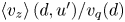 $\left \langle v_z \right \rangle (d,u')/v_{q}(d)$. Figure 8 suggests that
  $\left \langle v_z \right \rangle \propto 1/u'$, together with some
  $d$ scaling, so that we consider
  $\left \langle v_z \right \rangle /v_{q}$ as a function of the bubble Froude number
 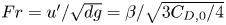 ${Fr} = u'/\sqrt {dg} = \beta / \sqrt {3 C_{{D},0} / 4}$ in figure 10 for various values of
  $d^*=d/L_{int}$.

Figure 10. The non-dimensional rise speed, binned by the size of the bubble in relation to the turbulent integral length scale  $d^*=d/L_{int}$, with the non-dimensional rise velocity
  $\left \langle v_z \right \rangle /v_{q}$ plotted against the non-dimensional intensity of the turbulence
  $u'/\sqrt {dg}$. Solid lines show data from our main experiment; the dotted line shows data from our second experimental set-up. The thicker line in the background shows
 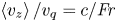 $\left \langle v_z \right \rangle /v_{q} = c/{\textit {Fr}}$, with
  $c=0.37$ an adjusted non-dimensional coefficient.
For all bubble sizes, bubbles in weak turbulence ( ${\textit {Fr}} \approx 0.25$ in our experiments) have a dimensionless average rise velocity reduced by a small factor, and we would expect
  $\left \langle v_z \right \rangle \rightarrow v_{q}$ for
  ${\textit {Fr}} {\rightarrow 0}$. As the turbulence is increased, the dimensionless average rise velocity decreases. Moreover, bubbles of all sizes (with
  $d^*$ from 0.07 to 0.4, so that all bubbles considered are within the inertial range of the turbulence) behave in the same way. The data collapse for various
  $d^*$, and at larger
  ${\textit {Fr}}$ scale as
 \begin{equation} \left \langle v_z \right \rangle/v_{q} = c / {\textit{Fr}}, \end{equation}
with  $c$ a non-dimensional coefficient fitted to the data,
  $c=0.37$. As will be discussed in the following section, this scaling will also be observed in point-bubble simulations, and will be justified with a theoretical model based on the role of the nonlinear drag and large-scale fluctuations in reducing the bubbles' rise velocity. This scaling and collapse in
  $d^*$ is also supported by the results from our second experiment, which are shown as the dotted green line. This experiment involved smaller bubbles and a shorter typical integral length scale, leading to larger values of
  $d^*$.
4. Point-bubble simulations in homogeneous, isotropic turbulence
Our experimental dataset shows that bubbles of all sizes (within the inertial range) are on average slowed by the turbulence, but it does not provide any information about the instantaneous flow field around the bubbles, in particular the slip velocity. To fill this gap, we carry out simulations of ‘point’ bubbles by solving the Maxey–Riley equation of motion for an inertial bubble in homogeneous, isotropic turbulence (HIT). In the Maxey–Riley paradigm, the fluid forces acting on the particle surface are replaced by effective added mass, drag and lift forces, which take into account some of the finite-size effects. While computationally easy to carry out using the output of a HIT simulation, two important aspects are not resolved with this approach. First, the bubble exerts no feedback onto the carrier fluid and is therefore advected passively. Second, the interaction with the turbulent background flow only depends on the bubble velocity and continuous phase conditions at the bubble centre. Doing so, the temporal variations of added mass, lift and drag are neglected, as well as their coupling with small scale statistics such as the velocity gradients.
Note that we consider a HIT flow, a canonical form of turbulence, for which the statistical properties have been extensively studied and described both experimentally and theoretically. The point-bubble approach does not capture some effects related to the finite size of the bubbles, in particular, the spatial averaging operation of fluctuations at a scale smaller than the bubble size. Previous works have quantified and characterized these finite-size effects in turbulence, in particular on the accelerations of particles of varying sizes larger than the Kolmogorov scale and densities close to the fluid density (Voth et al. Reference Voth, La Porta, Crawford, Alexander and Bodenschatz2002). The authors found that larger particles exhibited lower acceleration variances. Calzavarini et al. (Reference Calzavarini, Volk, Bourgoin, Lévêque, Pinton and Toschi2009) and Prakash et al. (Reference Prakash, Tagawa, Calzavarini, Mercado, Toschi, Lohse and Sun2012) applied Faxén corrections to the point-bubble equation of motion, in which the fluid velocity in the linear drag term is replaced with the average of the fluid velocity around the spherical particle's surface, and the fluid pressure term instead involves the average pressure over the particle volume, leading to good agreement with experimental measurements of particle accelerations.
As such, the instantaneous force acting on the bubble in the numerical simulation will be different from the experimental case, due to the averaging operation that takes place experimentally. However, we focus here on the large-scale statistics, namely the mean rise speed and the distribution of  $v'$. As we will see, the fluctuations of
  $v'$ are mainly Gaussian, both experimentally and numerically. This implies that the r.m.s. value of
  $v'$ is set by large-scale processes that do not necessarily require an accurate description of the influence of small-scale fluctuations. Here, we aim at exploring the role of nonlinear drag, which may play a greater role than the Faxén corrections in setting the mean rise velocity. We will also focus on the cross-statistics of the slip velocity
  $\boldsymbol {v}-\boldsymbol {u}$ and rise velocity
  $\left \langle v_z \right \rangle$. Experimentally, the rise velocity may be influenced by other factors such as deformability, which cannot be captured by any point-like simulation.
4.1. Simulation methodology
We employ the DNS of HIT publicly available on the Johns Hopkins Turbulence Database (Perlman et al. Reference Perlman, Burns, Li and Meneveau2007; Li et al. Reference Li, Perlman, Wan, Yang, Meneveau, Burns, Chen, Szalay and Eyink2008). The turbulence, generated by a random forcing in Fourier space, is described by the time-averaged Taylor-scale Reynolds number 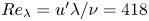 ${Re}_\lambda = u' \lambda / \nu = 418$ and large-scale Reynolds number
  ${Re}_{t} = u' L_{int} / \nu = 5060$, and is simulated on a
  $1024^3$ periodic grid spanning
  $L_{DNS} = 4.6 L_{int} = 2200 \eta$ in all three directions. For each condition simulated,
  $n_{b} = 500$ to 2500 point bubbles are positioned randomly in the domain.
Their position in time is advanced with (1.9), the Maxey–Riley equation simplified for a bubble in a much denser liquid. In total, this presents four initial dimensionless parameters:  $C_{M}$,
  $C_{L}$,
  $\beta$ and
  $d^*$. The turbulence characteristics are fixed with a single DNS simulation; therefore, we do not study any turbulent Reynolds number effects, but will compare with experimental results.
Numerically, (1.9) is integrated using a forward Euler scheme, with the velocity of bubble  $i$ at timestep
  $t+1$ written as
 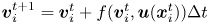 $\boldsymbol {v}_i^{t+1} = \boldsymbol {v}_i^{t} + f(\boldsymbol {v}_i^t,\boldsymbol {u}(\boldsymbol {x}_i^t)) \Delta t$, with
 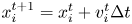 $x_i^{t+1} = x_i^t + v_i^t \Delta t$ the bubble position. The orientation of the coordinate system is chosen randomly for each bubble by picking an arbitrary direction for gravity with respect to the DNS;
  $\boldsymbol {e}_z$ is then defined to be anti-parallel to this direction. The timestep
  $\Delta t$ for most simulations is 5 times that used in the original DNS of the turbulence, giving
  $\Delta t \approx \tau _\eta / 40$. The integration was run with twice or half this value of
  $\Delta t$ for one case to ensure that results were converged with respect to
  $\Delta t$. Python code for the integration of the equation of motion is available at https://github.com/DeikeLab/point-particles-in-a-flow.
In all the simulations, we consider  $C_{M}=0.5$, the value for a solid sphere (Magnaudet & Eames Reference Magnaudet and Eames2000). As the lift coefficient is not yet well defined for deformable bubbles in turbulence, we initially vary its value between
  $-0.25$ and
  $0.25$ to assess its influence (Magnaudet & Eames Reference Magnaudet and Eames2000; Salibindla et al. Reference Salibindla, Masuk, Tan and Ni2020), and later fix
  $C_{L}=0$ as we observe the lift force does not have a strong impact on the results. Finally, we fix
  $C_{D}=1$, prescribing a constant ratio between
  $\beta$ and
  ${\textit {Fr}}$ for the point bubbles (
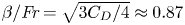 $\beta /{\textit {Fr}} = \sqrt {3 C_{D} / 4} \approx 0.87$). The use of a mean drag coefficient is questionable in particular because the instantaneous particle Reynolds number
  ${Re}_{p} = |\boldsymbol {v}-\boldsymbol {u}|d/\nu$ can vary significantly with time. Section 5.4 investigates the effect of a variable drag coefficient by computing
  ${Re}_{p}$ at each timestep, and then setting the drag coefficient accordingly following Snyder et al. (Reference Snyder, Knio, Katz and Le Maître2007). Figure 11 shows the
 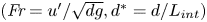 $({\textit {Fr}}=u'/\sqrt {dg}, d^*=d/L_{int})$ parameter space of the experiments and the point-bubble simulations, the latter of which were all carried out at
  $d^*=0.12$. In the rest of the paper, we will focus on the role of
  ${Fr}$ in setting the rise velocity.

Figure 11. The simulation conditions. (a) The relation between  ${Fr}$ and
  $d^*$. The joint probability density function (p.d.f.) of experimentally sampled conditions is shaded in the background. Orange markers denote the conditions simulated and discussed later in this paper. (b) A simulated three-dimensional bubble trajectory. (c) The vertical components of the bubble's velocity
  $\boldsymbol {v}$ (red) and the instantaneous fluid velocity at the bubble's location
  $\boldsymbol {u}$ (black). Times are normalized by the Eulerian integral time scale of the turbulence
  $L_{int}/u'$. The inset focuses on a region lasting approximately
  $0.4 L_{int}/u'$, and includes a horizontal black bar denoting the Kolmogorov time scale
  $t_\eta$.
First, to gain a qualitative insight into the bubble's interaction with the turbulence, we consider the simulations with two values of  $\beta$ (or Fr) depicted in figure 12. In each snapshot, the size of the field of view is proportional to the bubble size, and the carrier velocity field
  $\boldsymbol {u}$ is scaled by the quiescent rise velocity. The two panels, then, represent the same view of two bubbles, each of the same size and existing under the same gravitational acceleration (and therefore with the same
  $v_{q}$), but rising through turbulence fields with differing
  $u'$ (but the same
  $L_{int}$ and
  ${Re}_{t}$).

Figure 12. Snapshots of the carrier fluid velocity field in the  $x$–
$x$– $z$ plane coincident with the point bubble, normalized by
  $v_{q}$, (red background) and bubble trajectory (black lines) for two values of
  $\beta$ with
  $d^*=0.1$. The images are scaled such that the bubble size
  $d$ and gravitational acceleration
  $g$ can be treated as constant in both scenarios, while
  $u'$ varies to modify
  $\beta$.
  $C_{D}=1$ is used to prescribe the size of the point bubble in the image.
The magnitude of the turbulent velocity fluctuations in the carrier fluid increases with  $\beta$: the right snapshot, with
  $\beta =0.75$, presents a wider range of
  $|\boldsymbol {u}|$ than the left snapshot, with
  $\beta =0.25$. The bubble trajectories, too, exhibit markedly different characteristics. For the weakest turbulence case shown in the left, the bubble quickly passes through the fixed field of view, gradually curving in one direction but largely unaffected by the surrounding turbulence. When the velocity scale of the turbulence is larger, the bubble's trajectory exhibits tighter curvatures and takes on a more chaotic path. We will see that this is due to a relative increase of slip velocity compared with the mean rise velocity.
4.2. Comparison to experimentally measured velocities
We consider simulations run with  $d^*=0.12$, which is a typical value realized in the experiments (see figure 11). For now, we omit the lift force by setting
  $C_{L}=0$, but will later show it has only a small impact on the point-bubble average rise velocity. Figure 13 shows, for two values of
  $\beta$, the distributions of the normalized bubble vertical velocity
  $v_{z}/v_{q}$ as the solid red lines. The distribution of experimentally measured vertical bubble velocities for bubbles at similar conditions (considering
  $\beta$ within 0.1 and
  $d^*$ within 0.04 of the given values) are shown with the solid black lines, without any adjustable parameters. The experimental and numerical probability distribution functions show similar shapes, while experimental results present a slightly higher skewness, especially at low
  $\beta$. However, the general quantitative agreement in terms of the mean velocities and widths displayed by the p.d.f.s is very encouraging. The differences between the two can be attributed in part to the binning procedure used in selecting which experimentally measured points to include in the distribution, while the simulation involves a single, well-defined condition.

Figure 13. Experimentally measured (black) and simulated (red) velocity distributions for bubbles in turbulence. Red lines show distributions from the point-bubble simulation with  $\beta =0.5$ (a) or
  $\beta =1$ (b), with
  $d^*= 0.12$ and
  $C_{L}=0$. The corresponding values of
  ${\textit {Fr}}$ are 0.58 and 1.15. Black lines show the experimental measurements considering
  $\beta$ within 0.1 of the given value, and
  $d^*$ within 0.04 of
  $d^*=0.12$. Both the experimental and simulated distributions of the Eulerian fluid velocity are approximately Gaussian, and the measured distribution of bubble vertical velocities matches the shape of the simulated point-bubble vertical velocities.
Additionally, we show the simulated Eulerian distribution of carrier-phase velocity,  $u_z/v_{q}$, as the dotted red lines. This is created by randomly sampling the DNS at many locations and points in time. The analogous distribution from the experiments is obtained from the PIV results. While a slight up–down anisotropy is present in our experiment, the velocity p.d.f.s in the experiment and simulations are similar.
From the numerical simulations, we now have access to the statistics of the instantaneous liquid velocity at the bubble's location. Figure 14 shows the simulated distributions of the vertical and horizontal components of  $\boldsymbol {v}$,
  $\boldsymbol {u}$ (as sampled by the bubbles) and
  $\boldsymbol {v}-\boldsymbol {u}$ (each normalized by
  $u'$) for point bubbles at various
  $\beta$ and
  $d^*=0.12$. In weaker turbulence (
 $\beta =0.5$), the vertical slip
  $v_z-u_z$ (dashed lines) follows a more narrow distribution centred near
  $v_{q}$, but with a larger negative tail: the bubbles are typically rising through the carrier fluid with a relative velocity comparable to their quiescent rise velocity, but are slipping at lesser vertical velocities more often than they are at greater vertical velocities. The vertical fluid velocity the bubble samples
  $u_z$ (dash-dotted lines) has a distribution close to that of the Eulerian velocity field, centred near 0 with a dimensionless standard deviation of
  $u_z/u' \approx 1$. The bubbles’ absolute vertical velocity (solid lines), then, is centred near but below
  $v_{q}$, with a spread comparable to the spread in
  $u_z$.

Figure 14. Simulated vertical (a–c) and horizontal (d–f) velocity distributions for bubbles at various  ${\textit {Fr}}$ (columns), all normalized by
  $u'$. The distributions of normalized bubble velocity
  $v_i/u'$ are shown as the solid lines; the distributions of Lagrangian normalized carrier fluid velocity sampled by the bubbles
  $u_i/u'$ are shown as the dashed-dotted lines; and the distributions of bubble normalized slip velocity
  $(v_i-u_i)/u'$ are shown as the dashed lines, exhibiting exponential tails. The thicker orange curve in the background gives the Gaussian distribution corresponding to the mean and standard deviation of the bubble normalized velocity
  $v_i/u'$. The skewness of the distributions of
  $v_z$ are
  $-0.29$ for
  $\beta = 0.5$,
  $-0.02$ for
  $\beta = 1$ and 0.02 for
  $\beta =3$.
As  $\beta$ increases, the distribution of vertical fluid velocities
  $u_z$ sampled remains near Gaussian, with the standard deviation of
  $u_z/u' \approx 1$. Since the distributions of the vertical slip velocity
  $v_z - u_z$ are centred at or near
  $v_{q}$, this increased spread in
  $u_z$ increases the spread in the bubble's absolute vertical velocity,
  $v_z$. The distributions of the bubble's vertical slip velocity are asymmetric, in that fast upwards fluctuations are less likely than fast downwards fluctuations. As with the distributions of experimentally measured vertical velocities shown in figure 7, the skewness (reported in the caption) is more negative for smaller
  $\beta$ than for larger
  $\beta$. The spread in
  $v_z-u_z$ increases when
  $d^*$ increases.
The horizontal velocity distributions, when normalized by  $u'$, do not vary much with
  $\beta$ and are mostly Gaussian. The horizontal slip velocity also presents exponential tails, but is now centred on 0 for all values of
  $\beta$.
Having analysed the distributions of the bubble velocities and the fluid velocities they sample, we now consider the mean velocities with which they rise through the turbulence,  $\left \langle v_z \right \rangle$, which are shown alongside experimental data in figure 15. We vary
  ${\textit {Fr}}$ between 0.1 and 3.5 in our point-bubble simulations, and to assess the impact of the lift force, we consider
  $C_{L} = -0.25$, 0 and 0.25 with
  $d^*=0.12$. The mean rise speed, normalized by the quiescent rise speed, is shown in figure 15(a), plotted as a function of
  ${\textit {Fr}}$. The value of the lift coefficient has a negligible impact on the mean rise speed.

Figure 15. Experimental (solid coloured lines, binned by  $d^*$) and simulation results (at
  $d^*=0.12$). Points denote the dimensionless rise speed of the bubbles, for
  $C_{L}=-0.25$ (dash-dotted black line),
  $C_{L}=0$ (solid black line) and
  $C_{L}=0.25$ (dashed black line). Solid coloured lines (and the single dotted line from the second experiment) show the experimental results for different values of
  $d^*$. (a) The dimensionless rise speed plotted against the Froude number. The thicker orange line represents the
 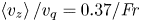 $\left \langle v_z \right \rangle / v_{q} =0.37/{\textit {Fr}}$ scaling. (b,c) The standard deviations of the horizontal and vertical bubble velocity fluctuations, respectively, normalized by
  $u'$.
$u'$.
We note that the values we consider for the lift coefficient are consistent with the ones reported by Salibindla et al. (Reference Salibindla, Masuk, Tan and Ni2020) in a turbulent flow. The negligible effect of the lift force within the Maxey–Riley framework is consistent with the work from Snyder et al. (Reference Snyder, Knio, Katz and Le Maître2007), who employed a more detailed lift coefficient that is dependent on the instantaneous local flow. The agreement between our experimental data and point-bubble simulations suggests that for the range of Weber number we consider (typically less than 1), the deformation is small enough so that the lift force will not have a significant effect. A detailed numerical study of the lift force effects would indeed require a much more sophisticated modelling approach.
To conclude, the numerical results are in good agreement with the collapse of the experimental data, which are shown again here for comparison. This confirms the experimentally observed scaling, 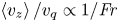 $\left \langle v_z \right \rangle / v_{q} \propto 1/{\textit {Fr}}$, valid for
  ${\textit {Fr}}\geqslant 0.4$, while a quadratic scaling for the decrease in rise velocity at low Froude number could represent the numerical data.
Figure 15(b,c) shows the standard deviation of the bubble horizontal and vertical velocities, respectively, as functions of the Froude number. In the point-bubble simulations, both components are near  $u'$. In the experimental data, bubbles at smaller
  ${\textit {Fr}}$ exhibit slightly greater velocity fluctuations than the turbulence, which might be attributed to bubble oscillations and deformability. Simulation results from Spelt & Biesheuvel (Reference Spelt and Biesheuvel1997) also indicate
  $v_z'/u'>1$ for bubbles at intermediate
  $\beta$ (which in their case are subjected to viscous drag), as did experiments from Mathai et al. (Reference Mathai, Huisman, Sun, Lohse and Bourgoin2018) at low
  $\beta$ (attributed to the bubble oscillations), although we leave open the possibility that our results are influenced by the heterogeneity of our experiment, which may cause bubbles to ‘carry’ with them large fluctuation velocities as they leave regions of large
  $u'$ and enter regions of lower
  $u'$. However, for
  ${\textit {Fr}} > 0.5$, our results indicate that the bubble velocity fluctuations can be attributed to the turbulent flow in which they are submersed.
4.3. Forces acting on the bubble
The mean values of the vertical component of the lift, drag and pressure forces acting on the point bubbles, each normalized by the vertical component of the buoyancy force 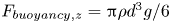 $F_{{buoyancy},z}={\rm \pi} \rho d^3 g/6$, are shown in figure 16(a). The forces are sketched for a bubble in a representative flow field in figure 16(b). At low values of
  ${\textit {Fr}}$, gravity is balanced by the drag force, and the lift and pressure forces are insignificant. (Without any turbulence, when
  ${\textit {Fr}}=0$, only the drag force is present in (1.9) to counteract buoyancy.) As
  ${\textit {Fr}}$ increases, the pressure term becomes significant, and in the
  $C_{L} \neq 0$ cases, the mean vertical lift force grows in magnitude. This mean lift force is upwards for
  $C_{L}=0.25$ and downwards for
  $C_{L}=-0.25$. Even though the lift force acts upwards on average in the
  $C_{L}=0.25$ case, it causes bubbles to be slowed to an even greater extent, due to its effect on the preferential sampling of the flow by the bubbles.

Figure 16. Forces acting on the bubble for  $d^*=0.12$. (a) The mean value of the vertical component of each force acting on the bubble at each condition, normalized by the gravitational force, for the constant
  $d^*$ cases shown in figure 15. Dash-dotted blue lines correspond to simulations with
  $C_{L}=-0.25$, solid black lines to
  $C_{L}=0$ and dashed red lines to
  $C_{L}=0.25$. (b) A sketch of a bubble (white) moving through a carrier fluid whose speed is shown in the image background. The instantaneous buoyant (green), lift (brown), drag (orange) and pressure (purple) forces acting on the bubble according to
  $\boldsymbol {v}$ and
  $\boldsymbol {u}$ are sketched.
An important result of these simulations is that, even though the turbulence through which the bubbles rise is homogeneous and isotropic, the pressure term 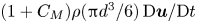 $(1+C_{M}) \rho ({\rm \pi} d^3 / 6) \,\mathrm {D} \boldsymbol {u} / \mathrm {D} t$ does not average to
  $\boldsymbol {0}$ over a bubble's trajectory. Instead, we see
 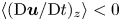 $\left \langle (\mathrm {D} \boldsymbol {u} / \mathrm {D} t)_z \right \rangle < 0$, meaning that it acts on average in the downwards direction, due to the bubbles’ preferential sampling of the flow. At larger
  $\beta$, this term plays a significant role in slowing the bubble down. Further, the means of the vertical drag and pressure forces display similar trends with or without the lift force present, and for
  ${\textit {Fr}}>1$, the ratio between drag and pressure forces appears constant.
Along with considering the mean values of forces acting on the bubbles, we can consider the mean values of the vertical fluid velocity sampled by the bubble  $\left \langle u_{z} \right \rangle$, the mean vertical slip velocity
  $\left \langle v_z - u_z \right \rangle$, the mean magnitude of the entire slip velocity
  $\left \langle |\boldsymbol {v} - \boldsymbol {u}| \right \rangle$, and the mean magnitude of the fluctuation component of the slip velocity
  $\left \langle |\boldsymbol {v}' - \boldsymbol {u}'| \right \rangle$, which are shown in figure 17, each normalized by
  $v_{q}$. The mean value of the vertical fluid velocity sampled by the bubbles
  $\left \langle u_z \right \rangle$, shown in blue, is typically slightly less than zero, but for higher
  ${\textit {Fr}}$, the mean slip velocity
  $\left \langle v_z-u_z \right \rangle$ is drastically decreased relative to the quiescent case, in which
  $v_z/v_{q}=1$. This reveals that the primary cause of the slowdown in rise velocity due to the turbulence is not the preferential sampling of
  $u_z<0$ regions, but is instead a decreased vertical slip velocity. Finally, at low values of
  ${\textit {Fr}}$, the magnitude of the slip velocity is given by the quiescent rise velocity, but at larger
  ${\textit {Fr}}$, it is dominated by the fluctuations in the slip velocity
  $\boldsymbol {v}'-\boldsymbol {u}'$. The typical magnitude of this slip scales linearly with
  $u'$. This presents an anisotropy in the mean slip velocity
  $\left \langle \boldsymbol {v}-\boldsymbol {u} \right \rangle$: at low
  ${\textit {Fr}}$, we have
 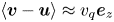 $\left \langle \boldsymbol {v}-\boldsymbol {u} \right \rangle \approx v_{q} \boldsymbol {e}_z$ (which is nearly
  $\left \langle v_z \right \rangle \boldsymbol {e}_z$ for such conditions), while at large
  ${\textit {Fr}}$, we have
  ${\left \langle \boldsymbol {v}-\boldsymbol {u} \right \rangle } \approx \boldsymbol {0}$ and
  $\left \langle |\boldsymbol {v}-\boldsymbol {u}| \right \rangle \approx u'$.

Figure 17. The mean value of the vertical fluid velocity  $u_z$, vertical slip velocity
  $v_z-u_z$, slip velocity magnitude
  $|\boldsymbol {v} - \boldsymbol {u}|$ and slip velocity fluctuation magnitude
  $|\boldsymbol {v}' - \boldsymbol {u}'|$, for point-bubble simulations with
  $d^*=0.12$. The mean vertical slip velocity
  $\left \langle v_z - u_z \right \rangle$ decreases to a much greater extent than that to which the bubble over-samples regions of
  $u_z < 0$. At low
  ${Fr}$, the magnitude of the slip velocity
  $|\boldsymbol {v}-\boldsymbol {u}|$ is dominated by the bubble's mean vertical slip
  $\left \langle v_z - u_z \right \rangle$, but at higher
  ${\textit {Fr}}$, becomes dominated by the fluctuations in the slip velocity
  $\boldsymbol {v}' - \boldsymbol {u}'$. The dashed black line gives a linear fit to
  $\left \langle |\boldsymbol {v}'-\boldsymbol {u}'| \right \rangle /v_{q}$ for
  $\beta \geqslant 0.5$.
5. Phenomenological model for weak and strong turbulence
To explain the transition from directional slip velocity to nearly isotropic slip velocity and the resulting trends in the average rise velocity, we propose a simple phenomenological model, based on the Maxey–Riley equation. We consider a bubble of diameter  $d$ immersed in a homogeneous and isotropic flow, determined by its r.m.s. velocity
  $u'$ and its integral length scale
  $L_{int}$. We consider the limits of negligible inertia of the gas phase (
 ${\rho _{p}} \ll \rho$) and an infinitesimally small particle. The use of an inertial drag force is justified by the quite large average Reynolds number at the bubble scale. In our experiments, the quiescent Reynolds number
  ${Re}_{q} = d v_{q} / \nu$, which serves as a lower bound for the mean particle slip Reynolds number
  ${Re}_{p} = d \left \langle |\boldsymbol {v}-\boldsymbol {u}| \right \rangle / \nu$, is between 50 and 1400. In our simulations, the values of
  ${Re}_{p}$ we calculate a posteriori are between 400 and 6000. As we will see, the nonlinearity of the drag force plays a crucial role in the evolution of the mean rise velocity with the turbulent intensity. With this inertial drag force, the bubble motion can be approximated by the Maxey–Riley equation (1.9), which we recall in dimensionless form
 \begin{equation} \alpha_1 d^* {\dot{\boldsymbol{v}}} = \alpha_2 d^* \left ( \partial_t + ({\boldsymbol{u}} \boldsymbol{\cdot} \boldsymbol{\nabla}) \right ){\boldsymbol{u}} + \frac{1}{\beta^2} {\boldsymbol{e}_z} - |\boldsymbol{v}-\boldsymbol{u}|(\boldsymbol{v} - \boldsymbol{u}),\end{equation}
where all velocities are here normalized by the r.m.s. velocity  $u'$,
$u'$,  $d^* = d/L_{int}$,
  $\beta = u'/v_{q}$,
  $v_{q}$ is the quiescent bubble velocity and
  $\alpha _1$ and
  $\alpha _2$ are numerical constants involving the drag and added-mass coefficients (see (1.9)). We neglect the contribution of the lift force. We have removed the
  $\tilde {\cdot }$ from the notation denoting dimensionless quantities for compactness and will specify when we return to dimensional quantities.
We introduce a Reynolds-type decomposition for  $\boldsymbol {v}$ and
  $\boldsymbol {u}$:
 \begin{equation} \boldsymbol{v} = v_0 {\boldsymbol{e}_z} + \boldsymbol{v}' \quad\text{and}\quad \boldsymbol{u} = \boldsymbol{u}',\end{equation}
since  $\left \langle \boldsymbol {v} \right \rangle \boldsymbol {\cdot } {\boldsymbol {e}_x} = \left \langle \boldsymbol {v} \right \rangle \boldsymbol {\cdot } {\boldsymbol {e}_y} = 0$ and
  $\left \langle \boldsymbol {u} \right \rangle = \boldsymbol {0}$, where the brackets
  $\left \langle \right \rangle$ stand for the average operation over bubble trajectory realizations. The average momentum terms such as
  $\left \langle ({\boldsymbol {u}} \boldsymbol {\cdot } \boldsymbol {\nabla }) {\boldsymbol {u}} \right \rangle$ can be non-zero even in a HIT flow, as shown from figure 16(a), due to the preferential sampling of the flow by the bubble. Introducing this decomposition into (5.1) and taking the ensemble average over the trajectory yields
 $$\begin{gather} \left \langle |\boldsymbol{v}-\boldsymbol{u}|(v_i - u_i) \right \rangle = \alpha_2 d^* \left \langle (\boldsymbol{u} \boldsymbol{\cdot} \boldsymbol{\nabla}) u_i \right \rangle, \quad i = x,y \end{gather}$$
 $$\begin{gather}\left \langle |\boldsymbol{v}-\boldsymbol{u}|(v_z - u_z) \right \rangle = \alpha_2 d^* \left \langle (\boldsymbol{u} \boldsymbol{\cdot} \boldsymbol{\nabla}) u_z \right \rangle + \frac{1}{\beta^2}. \end{gather}$$
The cornerstone of the behaviour of  $v_0$ lies in the expression of
  $|\boldsymbol {v}-\boldsymbol {u}|$. Using the Reynolds decomposition of
  $\boldsymbol {v}$, its square can be expressed as a sum of three contributing terms,
 \begin{equation} |\boldsymbol{v}-\boldsymbol{u}|^2 = v_0^2 + |\boldsymbol{v}'-\boldsymbol{u}'|^2 + 2 {\boldsymbol{e}_z} \boldsymbol{\cdot} (\boldsymbol{v}'-\boldsymbol{u}') v_0. \end{equation}
 The expression of  $\left \langle |\boldsymbol {v}-\boldsymbol {u}| \right \rangle$ can then be obtained in asymptotic cases, in which one of the terms is dominant. In the following, since
  $\left \langle {\boldsymbol {e}_z} \boldsymbol {\cdot } (\boldsymbol {v}'-\boldsymbol {u}') \right \rangle = 0$, we neglect the contribution of
  ${\boldsymbol {e}_z} \boldsymbol {\cdot } (\boldsymbol {v}'-\boldsymbol {u}')$ to
  $|\boldsymbol {v}-\boldsymbol {u}|$. We are left with two contributing terms,
 \begin{equation} |\boldsymbol{v}-\boldsymbol{u}| = \sqrt{v_0^2 + |\boldsymbol{v}'-\boldsymbol{u}'|^2}. \end{equation}
This defines two regimes, namely  $v_0 \gg |\boldsymbol {v}'-\boldsymbol {u}'|$, which corresponds to
  $\beta \ll 1$, and
  $v_0 \ll |\boldsymbol {v}'-\boldsymbol {u}'|$, which corresponds to
  $\beta \gg 1$. Qualitative differences between these two regimes can be seen by comparing the low-
 $\beta$ and high-
 $\beta$ (albeit with
  $\beta <1$) simulation snapshots in figure 12. The bubble velocity
  $\boldsymbol {v}$ at low
  $\beta$ is mainly dominated by the mean rise velocity
  $\left \langle v_z \right \rangle \boldsymbol {e}_z$, while the velocity fluctuations dominate the mean rise velocity for large
  $\beta$.
5.1. Case of $\beta \ll 1$: $v_0 \gg |{\boldsymbol {v}}-{\boldsymbol {u}}|$


In the  $\beta \ll 1$ limit, we expect the rise velocity to be only slightly perturbed by the presence of the background flow. In that regime, using
  $v_0 \gg |\boldsymbol {v}'-\boldsymbol {u}'|$, we have
  $|\boldsymbol {v}-\boldsymbol {u}| \approx v_0(1+({|\boldsymbol {v}'-\boldsymbol {u}'|^2})/{(2 v_0^2)})$ and, neglecting the convective term in (5.4) (
 $\beta \ll 1$), we obtain
 \begin{equation} \left \langle |\boldsymbol{v}-\boldsymbol{u}|(v_z - u_z) \right \rangle = v_0 \left( v_0 + \frac{\left \langle |\boldsymbol{v}'-\boldsymbol{u}'|^2 \right \rangle}{2 v_0} \right ) = \frac{1}{\beta^2}, \end{equation}
which yields  $v_0 = \sqrt {{1}/{\beta ^2} - \left \langle |\boldsymbol {v}'-\boldsymbol {u}'|^2 \right \rangle /{2}}$.
Using  $\left \langle |\boldsymbol {v}'-\boldsymbol {u}'| \right \rangle = \chi u'$ (which can be justified by figure 17), and recalling that with dimensions for
  $\left \langle v_z \right \rangle$ and
  $u'$ we have
  $v_0=\left \langle v_z \right \rangle /u'$,
  $\beta =u'/v_{q}$, we have the following dimensional result:
 \begin{equation} \left \langle v_z \right \rangle = v_{q} \left ( 1 - \frac{\chi}{4} \frac{u'^2}{v_{q}^2} \right). \end{equation}
This result is consistent with our numerical results shown in figure 15 at small  ${\textit {Fr}}$ (or small
  $\beta$), in that the slope of
  $\left \langle v_z \right \rangle /v_{q}$ goes to 0 as
  ${\textit {Fr}} \rightarrow 0$. Note that this result yields a reduction in rise speed quadratic in
  $\beta$, as does the analysis from Spelt & Biesheuvel (Reference Spelt and Biesheuvel1997) for small
  $\beta$, in which the constant is dependent on both the bubble's viscous response time and the size of the bubble in relation to the turbulence.
5.2. Case of $\beta \gg 1$: $v_0 \ll |\boldsymbol {v}'-\boldsymbol {u}'|$


In the second limit case, the main contribution to  $|\boldsymbol {v}-\boldsymbol {u}|$ originates from the fluctuation, i.e.
  $v_0 \ll |\boldsymbol {v}'-\boldsymbol {u}'|$. This yields
 \begin{equation} \left \langle |\boldsymbol{v}-\boldsymbol{u}| \right \rangle = \left \langle |\boldsymbol{v}'-\boldsymbol{u}'| \right \rangle + \frac{1}{2} \frac{v_0^2}{\left \langle |\boldsymbol{v}'-\boldsymbol{u}'| \right \rangle} + {O}(v_0^4). \end{equation}
The next hypothesis is to consider that the statistical properties of the fluctuations of the horizontal and vertical components of  $\boldsymbol {u}$ and
  $\boldsymbol {v}$ are similar (in other words, the fluctuations are decoupled from the mean). Equation (5.3) (for
  $u_i$,
  $i=x,y$) gives
 \begin{equation} \left \langle |\boldsymbol{v}-\boldsymbol{u}|(v_i' - u_i') \right \rangle = \alpha_2 d^* \left \langle (\boldsymbol{u} \boldsymbol{\cdot} \boldsymbol{\nabla}) u_i{'} \right \rangle, \end{equation}
which yields in the  $z$ direction
 \begin{equation} \left \langle |\boldsymbol{v}-\boldsymbol{u}| (v_z'-u_z') \right \rangle = \alpha_2 d^* \left \langle (\boldsymbol{u} \boldsymbol{\cdot} \boldsymbol{\nabla}) u_z{'} \right \rangle. \end{equation}
With these assumptions, we can replace the pressure term in the vertical momentum equation (5.4) with the fluctuations in the vertical drag force, yielding
 \begin{equation} \left \langle |\boldsymbol{v}-\boldsymbol{u}|(v_z - u_z) \right \rangle =\left \langle |\boldsymbol{v}-\boldsymbol{u}| (v_z'-u_z') \right \rangle + \frac{1}{\beta^2}. \end{equation}
Using  $v_z=v_0+v_z'$,
  $u_z = u_z'$ and (5.9), and keeping only the lowest order in power of
  $v_0$, we have
 \begin{equation} \left \langle |\boldsymbol{v}'-\boldsymbol{u}'| \right \rangle v_0 = \frac{1}{\beta^2}. \end{equation}
In dimensional form, this reads
 \begin{equation} \left \langle v_z \right \rangle = \frac{v_{q}^2}{\left \langle |\boldsymbol{v}'-\boldsymbol{u}'| \right \rangle}. \end{equation}
The final scaling of  $v_0$ depends on the value of
  $\left \langle |\boldsymbol {v}'-\boldsymbol {u}'| \right \rangle$ for large fluctuations compared with the bubble rise velocity. This relationship is confirmed with our point-bubble data in figure 18, which shows the dimensionless rise speed plotted against
  $\left \langle |\boldsymbol {v}'-\boldsymbol {u}'| \right \rangle /v_{q}$, at two values of
  $d^*$. Although the two curves do not collapse when plotted against
  ${\textit {Fr}}$ (in the inset), both exhibit the same relationship between the rise speed and the mean value of the fluctuations of the slip velocity magnitude.

Figure 18. The average dimensionless point-bubble rise speed as a function of  $\left \langle {|\boldsymbol {v}'-\boldsymbol {u}'|} \right \rangle / v_{q}$. (Inset) The non-dimensional rise speed plotted against the Froude number. Comparing the two plots shows that the mean value of the slip fluctuation speed sets the rise speed.
From figure 17, this magnitude scales as  $\left \langle |\boldsymbol {v}'-\boldsymbol {u}'| \right \rangle \propto u'$, set by an order-one constant that may depend on the bubble size
  $d^*$. On top of this, other size-dependent effects arise in the experiment which may not be captured by point-like simulations. For smaller
  $d^*$ the bubble dynamics should become highly intermittent, and the distribution of
  $|\boldsymbol {v}'-\boldsymbol {u}'|$ will both significantly decrease in magnitude and exhibit larger tails. The bubble deformation may also play an important role on the
  $d^*$ dependency of the bubble rise velocity.
Going back to the dimensional formulation, the high  ${\textit {Fr}}$ (or high
  $\beta$) regime leads to the following scaling for the bubble rise velocity:
 \begin{equation} \left \langle v_z \right \rangle \propto \frac{v_{q}}{{\textit{Fr}}}, \end{equation}
which is indeed the scaling observed for relatively high  ${\textit {Fr}}$ both in the experiments and point-bubble simulations in figures 10 and 15. This large Froude number scaling arises from the nonlinear drag force, which tends to make the slip velocity
  $\boldsymbol {v}-\boldsymbol {u}$ statistically isotropic and, as a consequence, reduces drastically the vertical slip velocity, henceforth the mean rise speed.
5.3. Bubble behaviour in a random Gaussian field
We note that our phenomenological model does not rely on flow features specific to HIT. As such, our results may be generalized to random flow fields which do not possess all the attributes of turbulent flows, as long as the typical bubble Reynolds number is sufficiently greater than 1 to yield a nonlinear relationship between the drag force and the slip velocity. To that end, we simulate the motion of point bubbles in a random Gaussian field composed of  $N$ Fourier modes following Mei (Reference Mei1994), where the fluid velocity
  $\boldsymbol {u}$ is defined as
 \begin{equation} \boldsymbol{u}(\boldsymbol{x},t) = \frac{1}{\sqrt{N}} \sum_{m=1}^N (\boldsymbol{b}^m \cos (\boldsymbol{k}^m \boldsymbol{\cdot} \boldsymbol{x} + \omega^m t) + \boldsymbol{c}^m \sin (\boldsymbol{k}^m \boldsymbol{\cdot} \boldsymbol{x} + \omega^m t)), \end{equation}
in which  $\boldsymbol {b}^m$,
  $\boldsymbol {c}^m$,
  $\boldsymbol {k}^m$ and
  $\omega ^m$ are picked from Gaussian distributions with 0 mean. The standard deviation of the distributions of
  $\boldsymbol {b}^m$ and
  $\boldsymbol {c}^m$ sets the large-scale velocity scale
  $u'$, the fluctuation velocity in HIT. The standard deviation of the distribution of the components
  $\boldsymbol {k}^m$ sets the large-scale length
  $1/k_0$, analogous to the integral length scale of the turbulence. Finally, the standard deviation
  $\omega _0 = u' k_0$ of the distribution of
  $\omega ^m$ sets the large-scale time scale
  $1/\omega _0$, analogous to
  $T_{int} = L_{int}/u'$ in HIT. We set the dimensionless bubble size to
  $d k_0 = 0.12$, and keep the constants in the Maxey–Riley equation equal to the values used in our main HIT simulations (
 $C_{D}=1$,
  $C_{M} = 0.5$,
  $C_{L}=0$).
The mean dimensionless rise velocity  $\langle v_z \rangle / v_{q}$ for these point bubbles in the Gaussian fields is shown as a function of
 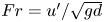 ${Fr} = u'/\sqrt {gd}$ in figure 19 as the solid black curve. As in HIT,
  $\langle v_z \rangle / v_{q}$ follows a
  $1/{Fr}$ scaling at large Froude number. Here, the scaling is more pronounced in the slip velocity
  $\langle v_z - u_z \rangle$ than in the mean rise velocity
  $\langle v_z \rangle$.

Figure 19. The mean rise velocity (black, solid line), mean magnitude of the slip velocity (cyan, dashed line) and mean vertical slip velocity (dark red, dotted line), of point bubbles in random Gaussian fields, with  $d k_0 = 0.12$ and varying
  ${Fr}$. At large
  ${Fr}$, the mean dimensionless rise velocity scales as
  $1/{Fr}$ (as does the mean vertical slip velocity, since the over-sampling of
  $u_z<0$ is negligible), and the mean magnitude of the slip velocity scales as
  ${Fr}$, congruent with our phenomenological model.
Further, the average magnitude of the slip velocity  $\langle | \boldsymbol {v} - \boldsymbol {u}| \rangle$ (shown in figure 19 as the dashed cyan curve) also scales with
  $u'$ in the Gaussian field. In both HIT and this random Gaussian field, the slowdown of the bubble due to the external flow is the result of the nonlinear drag force acting on the bubble. Since the fluctuation magnitude of the slip velocity increases linearly with
  ${Fr}$, the quadratic drag force along the vertical direction increases proportionally. From a balance with buoyancy force, the average bubble vertical velocity then decreases as
  $1/{Fr}$.
5.4. Point-bubble simulations with variable drag coefficient
To assess the use of a constant  $C_{D}$, we have run simulations of bubbles in random Gaussian fields using a time-varying drag coefficient, which is evaluated using the instantaneous bubble Reynolds number
  ${Re}_{p} = |\boldsymbol {v}-\boldsymbol {u}| d / \nu$. There is no general formula for the drag coefficient in an unstationary turbulent flow. Following Snyder et al. (Reference Snyder, Knio, Katz and Le Maître2007), we approximate the instantaneous drag coefficient by the value for a rigid sphere in a stationary flow of the same instantaneous Reynolds number, for which we have
 \begin{align} C_{D} &= \frac{24}{{Re}_{p}}, \quad {Re}_{p} < 1, \end{align}
 \begin{align} &= \left( \frac{24}{{Re}_{p}} \right) \left( 1 + \frac{3.6}{{Re}_{p}^{0.313}} \left( \frac{{Re}_{p} - 1}{19} \right)^2 \right), \quad 1 \leqslant {Re}_{p} \leqslant 20, \end{align}
 \begin{align} &= \left( \frac{24}{{Re}_{p}} \right) \left( 1 + 0.15 {Re}_{p}^{0.687} \right), \quad {Re}_{p} > 20. \end{align}
The viscosity  $\nu$ in the simulation is defined by matching the bubble Archimedes number
  ${Ar}= g d^3/\nu ^2$ to the corresponding values for an air bubble in water with
  $d=1$, 2 and 4 mm. For each value of
  ${Ar}$, we run simulations with a range of
  ${Fr}$ and
  $d k_0 = 0.1$.
The quiescent rise velocity is obtained for each condition by integrating the equation of motion using the variable drag coefficient with a quiescent velocity field. The same integration is then carried out using a random Gaussian field (as described in § 5.3), and the corresponding reduction in rise velocity is calculated. Finally, we calculate  $\langle C_{D} \rangle$ from this simulation, and run a final simulation using the version of the Maxey–Riley equation with constant coefficients (1.9) employed in our turbulent simulations, with
  $C_{D}$ fixed at this average value.
Results are shown in figure 20. Panel (a) shows that the variation itself in  $C_{D}$ does not have a large impact on the rise velocity, as the varying-
 $C_{D}$ and constant-
 $C_{D}$ curves for any
  $d$ nearly coincide. In other words, the use of a constant value of
  $C_{D}$ does not produce results significantly different than would be obtained with a time-varying
  $C_{D}$, provided that the constant value taken for
  $C_{D}$ is representative of the time-varying one. Panel (b) shows how, for fixed bubble sizes, the average value of
  $C_{D}$ changes with Froude number. As the Froude number is increased, the mean particle Reynolds number
  ${Re}_{p} = |\boldsymbol {v}-\boldsymbol {u}| d / \nu$ increases, and thus the average value of
  $C_{D}$ decreases from the quiescent value, due to the increased typical slip velocity. Thus, the variation of
  $\left \langle C_{D} \right \rangle$ with
  ${\textit {Fr}}$ may affect the scaling of
  $\left \langle v_z \right \rangle$ in a way that has not been considered in our phenomenological model. However, the exact variation of
  $C_{D}$ with the local Reynolds number
  ${Re}_{p}$ would require further analysis to be properly quantified, in particular in an unstationary, turbulent flow.

Figure 20. (a) Rise velocity for bubbles in random Gaussian fields with a variable drag coefficient  ${C}_D$ using the local Reynolds number
  ${Re}_{p}$ and the Snyder et al. (Reference Snyder, Knio, Katz and Le Maître2007) formulation (solid line). Dashed lines correspond to the case of a constant drag coefficient equal to the average value of the variable-
 $C_{D}$. Colours correspond to different bubble sizes (
 $d=1$, 2 and 4 mm). We observe no significant change in rise speed between the constant-
 $C_{D}$ and variable-
 $C_{D}$ formulations. (b) Time average drag coefficient
  ${C}_D$ as a function of the Froude number. The decrease of
  ${C}_D$ with the Froude number is attributed to the increase of the mean local Reynolds number
  ${Re}_{p}$, due to the increased typical slip velocity. (c) The p.d.f.s of
  $C_{D}$ for
  ${Fr}=0.7$, 3.1 and 13.0 for simulations with
  ${Ar}$ corresponding to
  $d=1\ \textrm {mm}$ (red) and
  $d=4\ \textrm {mm}$ (blue).
6. Discussion and conclusion
Having presented our experimental and simulation results, in this section we compare our results to those from the literature which report bubble rise speeds in turbulence. Figure 1, presented in the Introduction, gave the parameter space of these investigations, showing the size of the bubbles simulated relative to  $\eta$ and
  $L_{int}$, the non-dimensional turbulence intensity
  $\beta$, the turbulent Weber number
  ${We}$ and the quiescent Reynolds number
  ${Re}_{q}$. Figure 21 shows the rise velocity and non-dimensional change in speed due to the turbulence for our data and these additional studies. Experimental results for air bubbles in water are shown in dimensional terms in panel (a), in which the colour signifies
  $u'$. Panel (b) gives the dimensionless results as a function of the Froude number, in which the colour signifies
  $d^*$.

Figure 21. Comparison of results from various experiments, DNSs and point-bubble simulations. (a) Bubble rise speed as a function of the bubble size, with the colour scale denoting the turbulent fluctuation velocity  $u'$, for experiments involving air bubbles in water turbulence. The dashed lines show the rise velocity of air bubbles in quiescent water that is clean (the upper curve) and contaminated (the lower curve). (b) The non-dimensional rise velocity as a function of the Froude number for the experiments, DNSs, and point-bubble simulations. The thicker lines show the
  $\left \langle v_z \right \rangle /v_{q} = 1 - \chi \beta ^2/4$ relation at low
  ${\textit {Fr}}$ (using
  $C_{D}=1$ to specify
  $\beta$ and picking
  $\chi$ empirically) and the
  $\left \langle v_z \right \rangle /v_{q} = 0.37/\beta$ scaling at high
  ${\textit {Fr}}$.
The following four paragraphs briefly summarize the included data and explain how quantities were computed for each study. Aliseda & Lasheras (Reference Aliseda and Lasheras2011) report the bubble mean rise speed as a function of the bubble diameter  $d$ and the turbulent fluctuations
  $u'$. We aggregate data from their ‘large bubble’ and ‘small bubble’ datasets, but consider only the measurements with the lower void fraction from the ‘large bubble’ dataset, taking
  $L_{int}={2.5}\ \textrm {cm}$, the grid spacing in their experiment. Additionally, we do not consider their smallest bubbles, for which the large uncertainty in
  $v_{q}$ yields a substantial uncertainty in
  $\left \langle v_z \right \rangle /v_{q}$. Still, their bubbles are small enough that the drag exerted on them is dominated by viscosity. Poorte & Biesheuvel (Reference Poorte and Biesheuvel2002) report a non-dimensional slowdown of small bubbles due to weak turbulence, from which we calculate their mean rise speed. Prakash et al. (Reference Prakash, Tagawa, Calzavarini, Mercado, Toschi, Lohse and Sun2012) report the rise velocity as a function of
  ${Re}_\lambda$ for
  $d \approx 3\ \textrm {mm}$. Since they do not report
  $u'$ or
  $L_{int}$, we refer to a study from the same group using a modified version of the experiment (Mercado et al. Reference Mercado, Prakash, Tagawa, Sun and Lohse2012), from which we take
  $L_{int}={6}\ \textrm {cm}$ and interpolate
  $u'$ based on the reported value of
  ${Re}_\lambda$ (justified by the good agreement between the values of
  $\eta$ reported in Prakash et al. (Reference Prakash, Tagawa, Calzavarini, Mercado, Toschi, Lohse and Sun2012) and those interpolated from the Mercado et al. (Reference Mercado, Prakash, Tagawa, Sun and Lohse2012) data following the same approach). Salibindla et al. (Reference Salibindla, Masuk, Tan and Ni2020) report the mean rise speed as a function of
  $d$, holding the turbulence constant while changing the bubble size with
  $u'=0.25\ \textrm {m}\ \textrm {s}^{-1}$. The quiescent rise speed is calculated using the correlation for contaminated bubbles in quiescence from Clift et al. (Reference Clift, Grace and Weber1978) for all experimental datasets except Poorte & Biesheuvel (Reference Poorte and Biesheuvel2002), which reported the measured values, and Aliseda & Lasheras (Reference Aliseda and Lasheras2011), for which we use the relation for a dirty bubble from Park et al. (Reference Park, Park, Lee and Lee2017) (given the small bubble size).
DNSs of deformable bubbles from Loisy & Naso (Reference Loisy and Naso2017) are included as well, carried out at fixed  ${Bo} = g d^2 (\rho -{\rho _{p}}) / \sigma = 0.38$ and variable
  ${Ar} = \sqrt {g d^3 \rho (\rho -{\rho _{p}})}/\mu$, where
  ${\rho _{p}}$ is the density of the gas, with turbulence characterized by
  ${Re}_\lambda = 30$ and
  $\lambda = d$. We omit the DNS results from Reichardt et al. (Reference Reichardt, Tryggvason and Sommerfeld2017), who used a lower density ratio and
  ${Re}_\lambda < 10$.
We also include point-bubble simulation results in the dimensionless presentation of rise speed data in figure 21(b). Our point-bubble results, at  $d^*=0.12$ and
  $C_{L}=0$, are shown as the dash-dotted line. Data from Mazzitelli & Lohse (Reference Mazzitelli and Lohse2004) involve one condition of turbulence in which bubbles (experiencing viscous drag) of varying viscous response times
  $d^2/(24 \nu )$ and lift coefficients are simulated. The single case without lift, at
  ${\textit {Fr}} = 0.34$, is less slowed than the corresponding case with lift. Eight conditions from Snyder et al. (Reference Snyder, Knio, Katz and Le Maître2007), their ‘small bubbles’ and ‘large bubbles’, each simulated in four turbulent fields, are included, where we use the corresponding dimensional values they report to find
  $u'$ with
  $u' = \lambda / \sqrt {15 \nu / \epsilon }$ and
  $L_{int}$ with
  $L_{int} = {0.7} u'^3/\epsilon$.
Results from Salibindla et al. (Reference Salibindla, Masuk, Tan and Ni2020), who varied  $d$ in unchanging turbulence, stand out, as bubbles for which
  $d \geqslant 2\ \textrm {mm}$ yield an increase in rise speed relative to quiescent conditions. Their analysis attributed this to the modulation of the bubble lift and drag coefficients due to the turbulence's deformation of larger bubbles. This suggests that the turbulent Weber number, which until this point we have not considered, is important (Salibindla et al. Reference Salibindla, Masuk, Tan and Ni2020). However, our simulation results with positive and negative values of
  $C_{L}$ did not yield substantially different results. Nonetheless, we remark that our simulations do not account for deformation effects, which are certainly important for large bubbles (
 ${>}{4}\ \textrm {mm}$ in typical conditions) and could change the discussion on the importance of lift force. Additionally, we note the possibility of bubbles migrating preferentially to regions of varying mean flow according to their size in such an experiment, which may introduce an additional factor influencing their rise velocity. Figure 1 showed that the largest bubbles considered by Salibindla et al. (Reference Salibindla, Masuk, Tan and Ni2020) largely fall within the parameter space of our experiment, suggesting that the differences between our results for these large bubbles stem from the large-scale structure of the mean flow.
Despite the scatter in the compiled experimental and simulation data in figure 21(b), trends are consistent with the two asymptotic scalings presented in § 5. At low  $\beta$ (equivalently, low
  ${\textit {Fr}}$, as we now neglect variations in the drag coefficient), bubbles are slightly slowed relative to their quiescent rise, coherent with the
  $1-\left \langle v_z \right \rangle /v_{q} \propto \beta ^2$ scaling derived for
  $\beta \ll 1$. This
  $\beta ^2$ dependence is coherent with the analysis from Spelt & Biesheuvel (Reference Spelt and Biesheuvel1997), who for bubbles experiencing viscous drag at low
  $\beta$ found a prefactor dependent on the Taylor microscale of the turbulence and the bubble's viscous response time. At larger
  $\beta$ (larger
  ${\textit {Fr}}$), the dimensionless rise velocity decreases and approaches 0, coherent with the
  $\left \langle v_z \right \rangle /v_{q} \propto 1/{\textit {Fr}}$ scaling derived for
  $\beta \gg 1$. The scatter of points around these relationships suggests that the factors not captured in our point-bubble model, such as bubble finite-size effects, turbulent Reynolds number effects, bubble deformability and the instantaneous local flow field around the bubble, play a role in setting the average rise speed.
Additionally, the present experiments and those in the literature exhibit some large-scale inhomogeneities, which we partially account for in our analysis by subtracting the mean water flow from the observed bubble velocities. However, the impact on the average rise velocity of gradients in large-scale quantities such as  $u'$ remains an open question, together with the role of small-scale turbulence–interface interaction. Systematic experiments employing varying types of forcing which yield distinct inhomogeneities in the turbulence and DNSs fully resolving the bubble–turbulence interaction would help address these questions. Similarly, more involved point bubble simulations incorporating finite-size effects with Faxén corrections and drag, lift and added-mass coefficients dependent on the instantaneous flow field around the bubble, such as that carried out by Snyder et al. (Reference Snyder, Knio, Katz and Le Maître2007) (and in our § 5.4), would be a practical way to explore additional bubble-scale phenomena.
The  $1/u'$ scaling we derive and observe is relevant for bubbles experiencing nonlinear drag, for which the typical particle Reynolds number
  $\left \langle |\boldsymbol {v}-\boldsymbol {u}| \right \rangle d / \nu \gg 1$. A prerequisite, then, is that the quiescent Reynolds number
  ${Re}_{q}$, shown in figure 1, is also much greater than 1. For air bubbles in water, requiring
 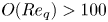 ${O}({Re}_{q}) > 100$ implies
 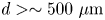 $d> \sim {500}\ {\mathrm {\mu }}\textrm {m}$. Similarly, as we have neglected the effects of severe bubble deformation and break-up, we require that the typical turbulent Weber number at the bubble scale,
  ${We} = 0.79 {Fr}^2 {Bo}\, {d^*}^{2/3}$, is not too large. Again looking to figure 1, we see that this parameter range (
 ${Re}_{q} \gg 1,{We} < 1$) is relevant for most of our dataset and most similar experiments.
In summary, we have performed experiments in which we measure the average speed at which air bubbles of various sizes rise through regions of turbulence of varying intensity in water. The decrease in rise speed relative to quiescent conditions that we measure is coherent with the rise velocity of point bubbles in turbulence, which we simulate numerically. At large Froude number  ${\textit {Fr}} = u'/\sqrt {gd}$, the dimensionless rise velocity scales as
  $\left \langle v_z \right \rangle /v_{q} \propto 1/{\textit {Fr}}$, which can be attributed to the nonlinearity of the drag force and the r.m.s. slip velocity being proportional to the turbulent intensity
  $u'$. Our experimental data collapse to a single average rise velocity curve over a range of
  $d^*=d/L_{int}$, but more extensive experiments and simulations are required to determine the influence of the turbulent length scales, bubble deformability, heterogeneities in the turbulence and interactions with non-zero-mean flows, which, among other things, may introduce dependencies on
  $d$ that we do not capture with our point-bubble analysis.
Funding
This work was supported by the NSF CAREER award 1844932 to L.D. We thank the Johns Hopkins database team for making their data available, and acknowledge the SciServer platform (Taghizadeh-Popp et al. Reference Taghizadeh-Popp2020), on which we carried out the point-bubble simulations.
Declaration of interests
The authors report no conflict of interest.
Appendix A. Experimental approximation of homogeneous, zero-mean turbulence
Our experiment is inhomogeneous at large scales, which enables us to observe bubbles in a variety of conditions in a single experiment. However, the flow seen by the bubbles is homogeneous, in that the time scales over which the statistics of quantities they probe change (in a Lagrangian sense, following the bubble) are longer than the time scales relevant to the bubbles’ dynamics.
A.1. Lagrangian time scales
To demonstrate this, for each measurement at a time  $t$ we directly compute the duration
  $\tau _{u'}$ over which the bubble has been within a region of
  $|u' - u'(\boldsymbol {x}_{b}(t))| \leqslant 0.05\ \textrm {m}\ \textrm {s}^{-1}$, since
  $0.05\ \textrm {m}\ \textrm {s}^{-1}$ corresponds to a typical size of a bin for
  $u'$. This definition of
  $\tau _{u'}$ is illustrated in figure 22(a): for time
  $t = {17.7}\ \textrm {s}$, denoted by the solid vertical line, the value of
  $u'$ is considered, shown as the solid circle. Next, the range of
  $u'$ within
  $\pm {0.05}\ \textrm {m}\ \textrm {s}^{-1}$ of this value is considered, denoted by the shaded region. The most recent time
  $u'$ was outside this range is then found, denoted by the dashed line. The difference between these two times is
  $\tau _{u'}(t)$.

Figure 22. The time scales over which the value of  $u'$ seen by the bubble changes. (a) The definition of
  $\tau _{u'}$, which is the duration over which the bubble has been in a region of
  $u'$ which is within
  $0.05\ \textrm {m}\ \textrm {s}^{-1}$ of its current value. (b) Cumulative distribution of
  $u'$ for bubbles as they are in regions of different turbulence intensities. (c) Cumulative distributions of
  $u'$ normalized by the integral time scale of the turbulence
  $T_{int} = L_{int}/u'$.
The values of  $\tau _{u'}$ are computed for each measurement, and the cumulative distribution of
  $\tau _{u'}$ is shown in figure 22(b) for various ranges of
  $u'$. Then, results are normalized by the local integral time scale
  $T_{int} = L_{int}/u'$, since the integral time scale sets the time over which the large-scale turbulent motions act on the bubble to slow its rise. The cumulative distribution functions of
  $\tau _{u'}/T_{int}$ are shown in figure 22(c). A bubble has been within a range of comparable
  $u'$ for at least half an integral time scale for
  ${\sim }80\,\%$ of measurements.
A.2. Insignificance of the mean flow field
A second consideration is the velocity gradients in the mean flow field, which through nonlinear drag may alter the bubble's rising velocity. Here, we show that the mean velocity gradients in our experiment are not strong enough to significantly impact the mean bubble rising speed, allowing us to attribute the observed reductions in rise velocity to the turbulence.
Since the PIV data provide two components of the mean flow velocity, we simulate the motion of a bubble constrained to a single, two-dimensional PIV plane, in which the flow field  $\boldsymbol {u}$ is taken to be the two known components of the mean flow,
  $\boldsymbol {u}(\boldsymbol {x}) = \bar {u}_x(\boldsymbol {x}) \boldsymbol {e}_x + \bar {u}_z(\boldsymbol {x}) \boldsymbol {e}_z$. The bubble trajectory is found by integrating (1.9), in which we neglect the pressure force by assuming the typical length scale of the mean flow is much greater than the bubble size. Figure 23 shows the results from one such simulation,

Figure 23. A simulation of a bubble with  $d=4\ \textrm {mm}$ in the mean flow field, initialized at an arbitrary position. (a,b) The trajectory superimposed over the mean horizontal and vertical flow fields, respectively. (c) The bubble's vertical slip velocity. The dashed line gives the quiescent rise velocity.
Figure 24 shows the simulated mean velocities of bubbles of various sizes in the mean flow, with close agreement to the quiescent rise velocity. Only times between 0.25 s after the bubble's initialization, and before it leaves the measurement volume, are considered. Further, the standard deviation of the bubble vertical velocities, denoted by the shaded red region, is significantly smaller than  $v_{q}$, letting us attribute the experimentally observed bubble velocity fluctuations to the turbulent fluctuations as well.

Figure 24. The mean simulated rise velocity of 40 bubbles of each size, each subjected only to the two measured components of the mean flow, initialized randomly within the PIV measurement volume. The dashed line gives the quiescent rise velocity, and the points are simulation results, all with  $C_{D}=1$. The agreement between the two curves suggests that gradients in the mean flow velocity are not responsible for the experimentally observed decrease in rise velocity in our experiment. The red shaded area shows one standard deviation of the bubbles’ vertical velocity above and below the mean.
Appendix B. Second experiment
Figure 25 shows the flow characteristics of our second experiment, in which we also measure the rise velocity of bubbles in turbulence. Like our main experiment, it involves pump-generated water turbulence, but does so at a smaller scale with two planes of opposing pumps. Results from this experiment are included as dotted lines.

Figure 25. Summary of PIV results from the second experiment. (a) From left to right, the mean flow, the fluctuations in the  $x$ and
  $z$ directions and integral length scale in three of the nine PIV planes. (b) The location of the nine PIV planes in the tank. The three coloured planes correspond to the three for which fields are shown above. (c) The integral of the autocorrelation function from which the integral length scale is calculated, at the three marked points. (d) The structure at a single point in each of the three planes, which are marked by an
  $x$ in the fields. (e) The compensated structure function. The dashed lines give estimates of the dissipation rate with
  $0.7u'^3/L_{int}$.


