1. Introduction
No method of forecasting earthquakes by the commonly used seismic measurements (SM) has yet been found (Bormann, Reference Bormann2011). The development of an earthquake usually takes place in three stages (Eftaxias & Potirakis, Reference Eftaxias and Potirakis2013): nucleation, stick-slip and a final drastic slip movement. At the nucleation stage, under the increasing stress amplitude, there appear many tiny fractures in the area around the existing fault (known as the ‘heterogeneous environment’). According to our model (Rabinovitch, Frid & Bahat, Reference Rabinovitch, Frid and Bahat2007), such tiny fractures emit high-frequency electromagnetic radiation (FEMR) pulses (of the order megahertz). Fractures increase in size progressively (but intermittently) during the stick-slip stage, when asperities of increasing size and strength are severed. The increased surface areas liberated give rise to FEMR pulses of ever-lower frequencies (Rabinovitch, Frid & Bahat, Reference Rabinovitch, Frid and Bahat2007); the reduction in FEMR frequency from megahertz to kilohertz may therefore herald the transition between these stages of the imminent earthquake. During the following drastic slipping mode of the earthquake, a dilation gap between the sides of the moving fault is established and no new surfaces are created (Eftaxias & Potirakis, Reference Eftaxias and Potirakis2013); it is expected that hardly any FEMR would be observed at this stage. The sequence of detected FEMR pulse frequencies during an earthquake follows the pattern: (1) multiple megahertz pulses related to tiny fractures; (2) multiple kilohertz pulses of decreasing frequencies related to larger and larger fractures (asperities breaking); such an FEMR pulse frequency sequence heralds the forthcoming earthquake; and (3) no FEMR pulses during the final earthquake stages.
The fractures at the early stages of an earthquake, characterized by frequencies of the order megahertz and kilohertz, cannot be detected by seismic means.
The attenuation of FEMR and seismic waves is treated individually; in this article, we only consider attenuation of plane waves. The energy of waves emanating from a confined source decays with distance r as 1/4πr 2 as well as the attenuation of plane waves.
2. FEMR attenuation
The attenuation of electromagnetic waves in any medium can be theoretically calculated by Maxwell's equations applied to the properties of the actual material which, in our case, are the lithospheric rocks (Zhang & Li, Reference Zhang and Li2007). We present here a short derivation of this calculation and use it to obtain the attenuation of dominant lithospheric rock types.
Maxwell's equations (in MKSA units) are:
 $$\begin{equation*}
\nabla \cdot {\bm{D}} = \rho
\end{equation*}$$
$$\begin{equation*}
\nabla \cdot {\bm{D}} = \rho
\end{equation*}$$
 $$\begin{equation*}
\nabla x{\bm{E}} = - \partial {\bm{B}}/\partial t
\end{equation*}$$
$$\begin{equation*}
\nabla x{\bm{E}} = - \partial {\bm{B}}/\partial t
\end{equation*}$$
 $$\begin{equation*}
\nabla \cdot {\bm{B}} = 0\
\end{equation*}$$
$$\begin{equation*}
\nabla \cdot {\bm{B}} = 0\
\end{equation*}$$
 $$\begin{equation*}
\nabla x{\bm{H}} = {\bm{j}} + \partial {\bm{D}}/\partial t
\end{equation*}$$
$$\begin{equation*}
\nabla x{\bm{H}} = {\bm{j}} + \partial {\bm{D}}/\partial t
\end{equation*}$$
where D is the electric displacement (C m–2), E is the electric field intensity (V m–1), B is the magnetic induction (T), H is the magnetic field intensity (A m–1), ρ is the charge density (C m–3) and j is the electric current density (A m–2).
For a homogeneous isotropic linear medium devoid of free currents and charges, we have:
 $$\begin{equation*}
{\bm{D}} = \varepsilon {\bm{E}};{\bm{\ B}} = \mu {\bm{H}};{\bm{j}} = \rho = 0
\end{equation*}$$
$$\begin{equation*}
{\bm{D}} = \varepsilon {\bm{E}};{\bm{\ B}} = \mu {\bm{H}};{\bm{j}} = \rho = 0
\end{equation*}$$
where ε = ε' + iε''is the complex electrical permittivity, μ is the magnetic permeability and σ is the conductivity, all of them being medium properties.
For the type of media described above, we therefore have:
 $$\begin{equation*}
\nabla x{\bm{E}} = - \mu \frac{{\partial {\bm{H}}}}{{\partial t}}{\rm{\ \ and\ \ }}\nabla x{\bm{H}} = \sigma {\bm{E}} + \frac{{\varepsilon \partial {\bm{E}}}}{{\partial {\rm{t}}}}.
\end{equation*}$$
$$\begin{equation*}
\nabla x{\bm{E}} = - \mu \frac{{\partial {\bm{H}}}}{{\partial t}}{\rm{\ \ and\ \ }}\nabla x{\bm{H}} = \sigma {\bm{E}} + \frac{{\varepsilon \partial {\bm{E}}}}{{\partial {\rm{t}}}}.
\end{equation*}$$
Taking the curl of each of the immediately above equations and inserting it into the other leads to:
 $$\begin{equation*}
{\nabla ^2}{\bm{E}} - \ \mu \sigma \frac{{\ \partial {\bm{E}}}}{{\partial {\rm{t}}}} - \mu \varepsilon {\partial ^2}{{\bf E}}/\partial {t^2} = 0
\end{equation*}$$
$$\begin{equation*}
{\nabla ^2}{\bm{E}} - \ \mu \sigma \frac{{\ \partial {\bm{E}}}}{{\partial {\rm{t}}}} - \mu \varepsilon {\partial ^2}{{\bf E}}/\partial {t^2} = 0
\end{equation*}$$
and
 $$\begin{equation*}
{\nabla ^2}{\bm{H}} - \ \mu \sigma \frac{{\partial {\bm{H}}}}{{\partial {\rm{t}}}} - \mu \varepsilon {\partial ^2}{{\bf H}}/\partial {t^2} = 0.
\end{equation*}$$
$$\begin{equation*}
{\nabla ^2}{\bm{H}} - \ \mu \sigma \frac{{\partial {\bm{H}}}}{{\partial {\rm{t}}}} - \mu \varepsilon {\partial ^2}{{\bf H}}/\partial {t^2} = 0.
\end{equation*}$$
For waves for which E and H are defined E 0 ei ω t and H 0 ei ω t , respectively, where ω = 2πf is the angular velocity, f is frequency and t is time, we have:
 $$\begin{equation}
{\nabla ^2}{{\bm{E}}_0} + {k^2}{{\bm{E}}_0} = 0{\rm{\ and\ }}{\nabla ^2}{{\bm{H}}_0} + {k^2}{{\bm{H}}_0} = 0
\end{equation}$$
$$\begin{equation}
{\nabla ^2}{{\bm{E}}_0} + {k^2}{{\bm{E}}_0} = 0{\rm{\ and\ }}{\nabla ^2}{{\bm{H}}_0} + {k^2}{{\bm{H}}_0} = 0
\end{equation}$$
where k 2 is the complex wave number, defined:
 $$\begin{equation}
{k^2} = {\omega ^2}\mu \varepsilon ' - i\left( {\omega \mu \sigma + \varepsilon ''} \right).
\end{equation}$$
$$\begin{equation}
{k^2} = {\omega ^2}\mu \varepsilon ' - i\left( {\omega \mu \sigma + \varepsilon ''} \right).
\end{equation}$$
For a wave which is linearly polarized in the x direction and moving in the z direction,
 $$\begin{equation*}
{{\bm{E}}_0} = {E_0}{e^{ - \gamma z}}\hat{x}{\rm{\ \ and\ \ }}{{\bm{H}}_0} = {H_0}{e^{ - \gamma z}}\hat{y}
\end{equation*}$$
$$\begin{equation*}
{{\bm{E}}_0} = {E_0}{e^{ - \gamma z}}\hat{x}{\rm{\ \ and\ \ }}{{\bm{H}}_0} = {H_0}{e^{ - \gamma z}}\hat{y}
\end{equation*}$$
where γ = α + iβ = ik; α is the attenuation constant; β is the phase constant; and
 $\hat{x}$
and
$\hat{x}$
and
 $\hat{y}$
are unit vectors in the x and y directions.
$\hat{y}$
are unit vectors in the x and y directions.
We assume (Korpisalo, Reference Korpisalo2014) that the polarization loss is small and conductivity is not negligible. We also assume that ωμσ >> ε″, and henceforth substitute ε for ε′.
Using Equations (1) and (2), the attenuation coefficient α (m–1) is:
 $$\begin{equation*}
\alpha = \omega \sqrt {\mu \varepsilon /2} {\left( {\sqrt {1 + {{\left( {\frac{\sigma }{{\omega \varepsilon }}} \right)}^2}} - 1} \right)^{{1
/ 2}}}.
\end{equation*}$$
$$\begin{equation*}
\alpha = \omega \sqrt {\mu \varepsilon /2} {\left( {\sqrt {1 + {{\left( {\frac{\sigma }{{\omega \varepsilon }}} \right)}^2}} - 1} \right)^{{1
/ 2}}}.
\end{equation*}$$
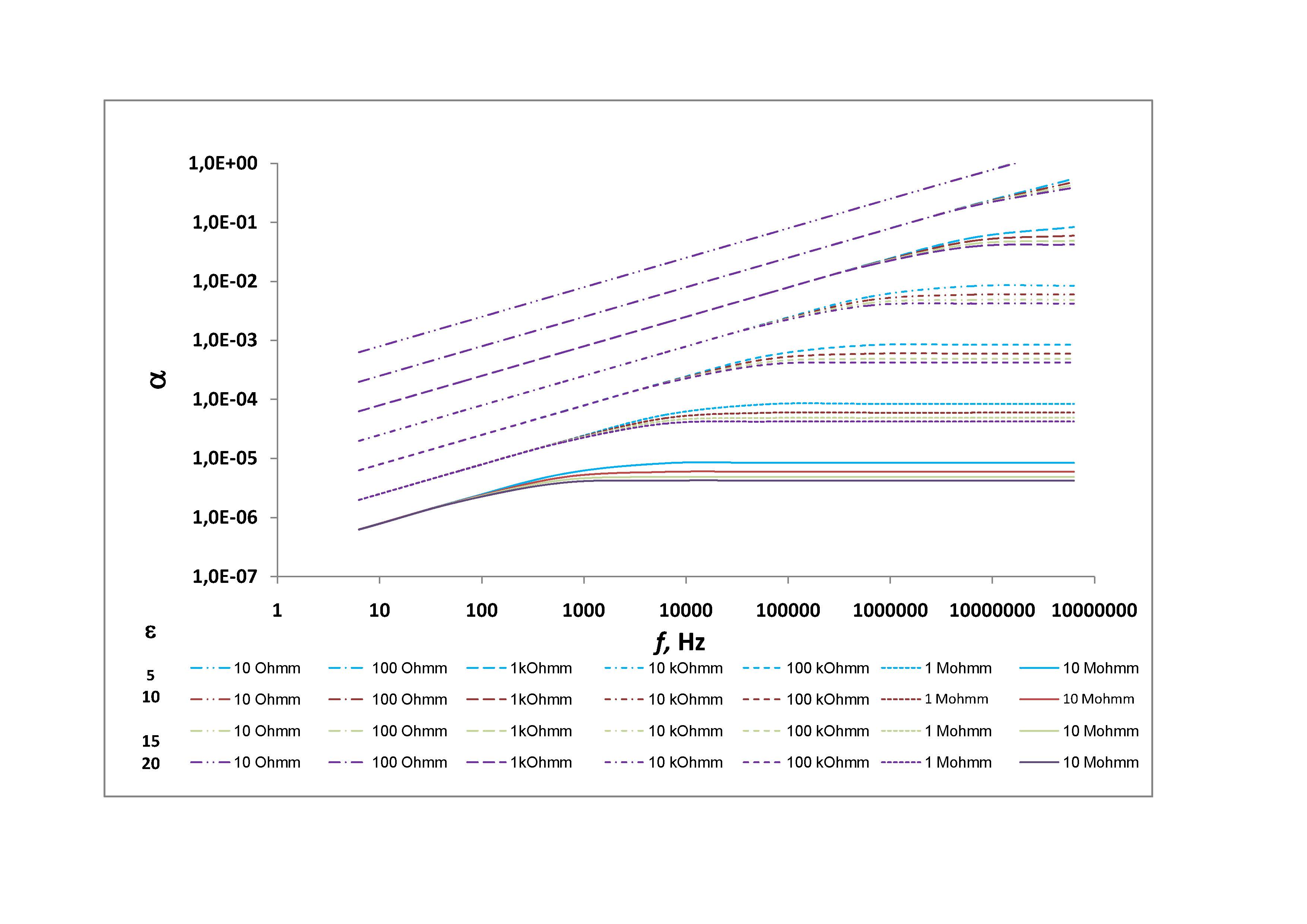
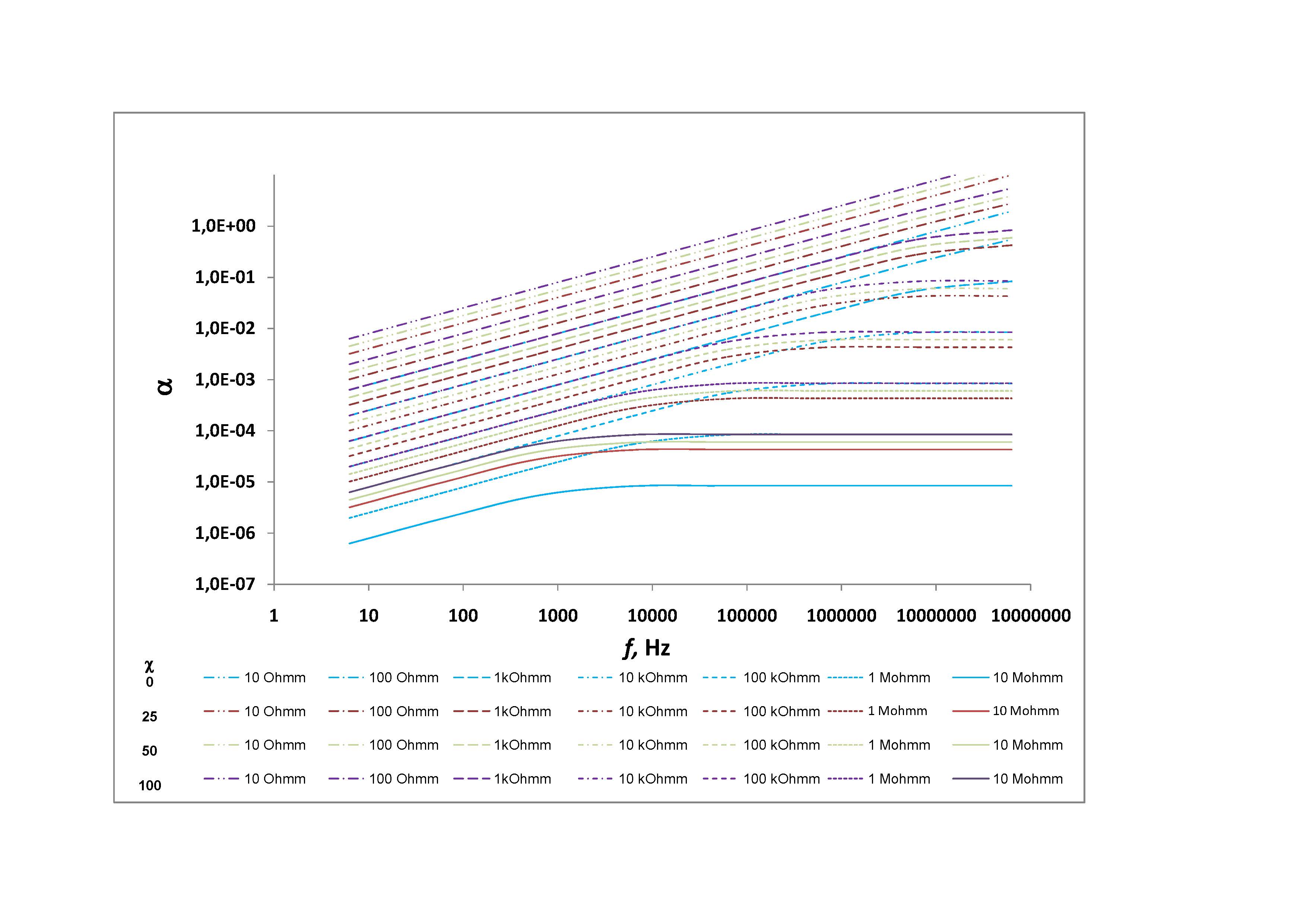
The permittivity, permeability and conductivity of the rocks where the most abundant earthquakes occur are given in Table 1 (Telford, Geldart & Sheriff, Reference Telford, Geldart and Sheriff1990). Note that μ = μ 0(1+χ), where χ is the dimensionless magnetic susceptibility and μ 0 = 4π×10−7 H m–1 is the permeability of free space, and ε = ε 0 ε r, where ε r is the dimensionless dielectric constant and ε 0 = 8.84×10⁻¹² F m–1 is the permittivity of free space.
Table 1. Typical rock electrical parameters (Telford, Geldart & Sheriff, Reference Telford, Geldart and Sheriff1990)

3. Acoustic emission attenuation
Attenuation of acoustic (seismic) emission (AE) in the Earth's crust, a function of distance (r) and frequency (f), is assumed to be conducted (Johnston, Toksöz & Timur, Reference Johnston, Toksöz and Timur1979; Menke, Levin & Sethi, Reference Menke, Levin and Sethi1995) under conditions of constant Q (s) (a rock-dependent property), at least for frequencies above 1–10 Hz and for dry rock. The amplitude A of the AE at a distance r from a plane-wave source of amplitude A 0 is defined:
 $$\begin{equation}
A\left( {f,r} \right) = {A_0}\exp \left( { - \alpha fr} \right)\
\end{equation}$$
$$\begin{equation}
A\left( {f,r} \right) = {A_0}\exp \left( { - \alpha fr} \right)\
\end{equation}$$
where α (m−1) is defined as π/Qv and v (m s–1) is the acoustic wave velocity (which is approximately a constant for either P- or S-waves). For a constant Q (s), α is therefore also a constant.
In the case of a concentrated source this amplitude is also proportional to 1/r since, as mentioned above, the energy which is proportional to A 2 decays as 1/4πr 2.
For liquid-saturated rocks, the use of the ‘wave-induced fluid flow’(WIFF) theoretical approach (Solazzi et al. Reference Solazzi, Rubino, Müller, Milani, Guarrcino and Hollinger2016) is usually applied to calculate AE attenuation. These calculations are also authenticated by experimental measurements. For such materials, 1/Q is no longer a constant. It changes as a function of frequency, showing a high peak at a specific wave frequency and decaying rapidly at both low and high wave frequencies. Regardless, attenuation for wet rocks is much higher than that for dry rocks; since it is presently shown that attenuation is already too great for the detection of seismic waves of high frequencies at longer distances, we consider here dry rocks only.
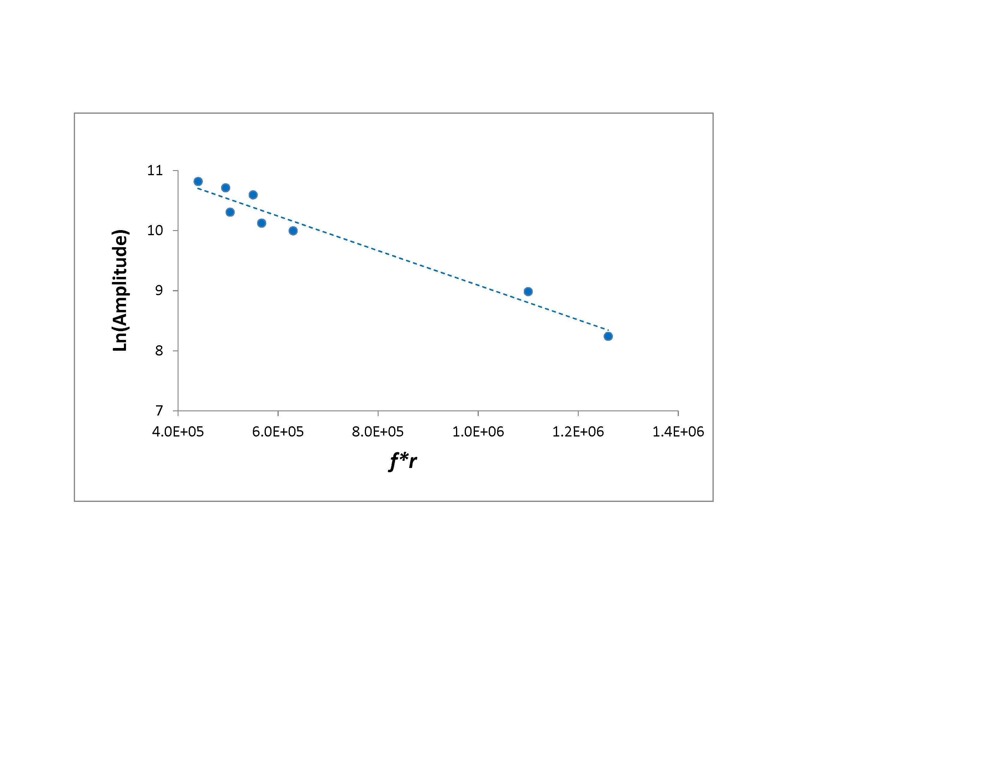
In order to derive physical values for the constant α, we make use of two different experimental results for two different rocks as follows. (1) Seismic measurements of several rather low frequencies were detected at specific distances from the centre of the Ladakh–Karakoram earthquake (Rai, Padhi & Sarma, Reference Rai, Padhi and Sarma2009). A modified figure 4 of Rai, Padhi & Sarma (Reference Rai, Padhi and Sarma2009) is shown here as online Supplementary Figure S1 (available at http://journals.cambridge.org/geo). Using this figure, we obtain α = 3×10⁻⁶ m–1. (2) For Navajo Sandstone at room temperature (porosity 12.5; Toksöz, Johnston & Timur, (Reference Toksöz, Johnston and Timur1979; see Table 1), for plane P-waves we have v = 4250 m s–1 and Q = 7.3 s; we therefore have α = 1.02×10⁻⁴ m–1 and Equation (4) becomes:
 $$\begin{equation*}
A = {A_0}\exp \left( { - \frac{{\pi fr}}{{vQ}}} \right){\rm{\ }} = {\rm{\ }}{A_0}{\rm{exp}}\left( { - 1.02{\rm{x}}{{10}^{ - 4}}fr} \right),
\end{equation*}$$
$$\begin{equation*}
A = {A_0}\exp \left( { - \frac{{\pi fr}}{{vQ}}} \right){\rm{\ }} = {\rm{\ }}{A_0}{\rm{exp}}\left( { - 1.02{\rm{x}}{{10}^{ - 4}}fr} \right),
\end{equation*}$$
where f is the frequency (Hz) and r is the distance (m).
The above results show that: (1) although in some rocks the attenuation of FEMR can be too high and may obscure the detection of high-frequency pulses at convenient distances from an EQ source, it was demonstrated (Fig. 1) that these pulses would generally arrive at the measuring device; and (2) on the other hand, AE (seismic) waves at frequencies of the order kilohertz and megahertz (Fig. 2) will not be able to reach such distances due to their higher attenuation.
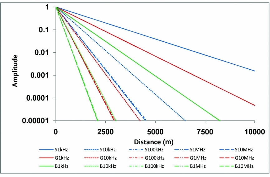
Figure 1. Attenuations (scaled amplitudes v. distance in m) of plane waves of FEMR as functions of frequency. Blue: sandstone; red: granite; green: basalt. Full line: 1 kHz; dashed line: 10 kHz; dot-dashed: 100 kHz; dashed-dot-dot-dashed: 1 MHz; extended dashed: 10 MHz. All attenuations are for averaged rock parameters. Extended attenuation figures for numerous EM parameters are included in the additional material to this paper (see online Supplementary Figs S2, S3, available at http://journals.cambridge.org/geo).
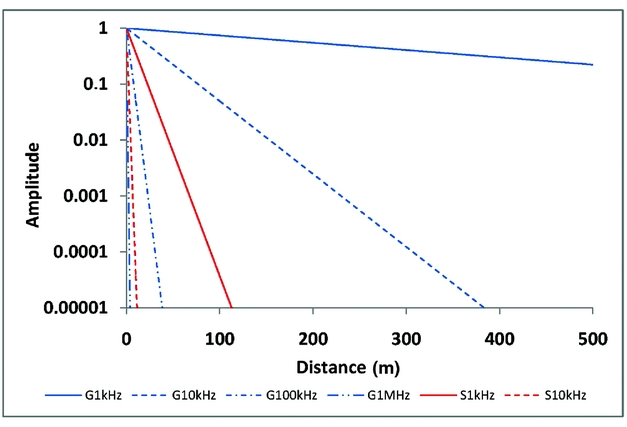
Figure 2. Attenuations (scaled amplitudes v. distance in m) of plane waves of AE as functions of frequency. Note the different scale from Figure 1. Red: sandstone; blue: granite. Full line: 1 kHz; dashed: 10 kHz; dot-dashed: 100 kHz; dashed-dot-dot-dashed: 1 MHz.
4. FEMR noise reduction
The main problem in detecting FEMR is the noise level of electromagnetic radiation from possibly many different sources. These obviously clutter the FEMR signal, making it sometimes impossible to detect. Based on our previous studies (see Appendix part A for a brief description of the measuring process), we suggest a method by which FEMR emitted by fracturing could be discerned from EMR emitted by other causes. As a result of these studies, we have established both experimentally and theoretically (Rabinovitch, Frid & Bahat, Reference Rabinovitch, Frid and Bahat2007) the structure of an FEMR pulse which is emitted from an evolving crack. Figure 3 depicts such a pulse, the amplitude of which first increases exponentially for a certain time (T – t 0, where T and t 0 are the times to the pulse envelope maximum and pulse origin, respectively) and then decays exponentially to zero. The main part is oscillatory with a specific frequency. We have shown that the increasing-amplitude time depends on the crack length and the frequency depends on the crack width. It was also demonstrated (Rabinovitch et al. Reference Rabinovitch, Frid, Bahat and Goldbaum2000; Rabinovitch, Bahat & Frid, Reference Rabinovitch, Bahat and Frid2002) that this shape is invariant to the fracture mode (tension, compression and shear) and to the loading mode (quasi-static and dynamic, e.g. drilling and quarry blasting). Fracture-initiated EM radiation is therefore composed of (multiple) single pulses of a specific shape, while EM radiation from other sources (e.g. radio waves, electronic machines) are usually continuous in time and/or do not follow the shape of Figure 3. We therefore suggest that the field-measured FEMR oscillations should be spread out in time until individual pulses can clearly be discerned; only if their emerging shapes resemble that depicted in Figure 3 should they be considered as originating from fractures and possibly related to the precursors of an earthquake. A method of analysing a single pulse to extract its specific parameters is presented in the Appendix (part B), and applied to an experimental example. For a case where multiple pulses coexist, we refer the interested reader to our papers on FEMR measured from a quarry explosion (Rabinovitch, Bahat & Frid, Reference Rabinovitch, Bahat and Frid2002; Goldbaum et al. Reference Goldbaum, Frid, Bahat and Rabinovitch2003) in which a mathematical method was developed to distinguish individual pulses from overlapping pulses. In addition, experience in FEMR investigations in underground conditions indicates that additional noise reduction can be obtained by placing antennae in underground tunnels (Frid & Vozoff, Reference Frid and Vozoff2005; Wang et al. Reference Wang, He, Liu and Wenquan Xu2012) or/and in boreholes (Fujinawa & Takahashi, Reference Fujinawa and Takahashi1998; Tsutsui, Reference Tsutsui2014). For a description of such measurements see the Appendix, part C.

Figure 3. The standard shape of an FEMR pulse. T–t 0, time of amplitude increase; ω, frequency.
5. Discussion
Attenuation alone is not sufficient to determine the output of a measuring device; the initial amplitude is also crucial. It is not easy to assess the amplitudes of either seismic or electromagnetic signals at their source. A recent paper (McLaskey & Lockner, Reference McLaskey and Lockner2016) deals with this problem in relation to seismic (acoustic) signals, and points out the difficulties encountered in their calibration. For an indication of these amplitudes, we recall that these come from the precursor stages of the earthquake and not from the actual earthquake event when, evidently, amplitudes are much higher. The cracks during these stages are quite small, and we can therefore compare their amplitudes to those obtained in laboratory experiments; for example, signals of amplitudes of up to 15 mV are measured in fractures in granite samples (McLaskey & Lockner, Reference McLaskey and Lockner2016). According to figure 7 of Rabinovitch, Frid & Bahat (Reference Rabinovitch, Frid and Bahat2007) the amplitudes of the electromagnetic signals measured near the cracks reach up to 1.5 mV. The amplitude ratio is therefore only of the order 10 in favour of the AE, which is not high enough to counteract the attenuation ratios.
Noise, or more accurately disturbances, in FEMR arises from two sources: man-made and natural. In an interesting paper by Koulouras et al. (Reference Koulouras, Balasis, Kiourktsidis, Nannos, Kontakos, Stonham, Ruzhin, Eftaxias, Cavouras and Nomicos2009), the authors successfully removed man-made disturbances by measuring earthquake precursors at several distributed locations and at several frequencies. They differentiated FEMR and VHF EMR emitted by natural causes by utilizing their fractal properties. We propose a different approach: noise associated with radiation is generally a continuous phenomenon, while FEMR is composed of singular pulses of the shape depicted in Figure 3. Since this shape is unique, identifying it and its parameters (see Appendix, part B) allows the true identification of FEMR in contrast to other sources.
Supplementary material
To view supplementary material for this article, please visit https://doi.org/10.1017/S0016756817000954
Appendices
Appendix A
The detailed description of the equipment used for our studies can be found in Rabinovitch, Frid & Bahat (Reference Rabinovitch, Frid and Bahat2007). Here we provide only a brief description of equipment. We used a triaxial load frame (TerraTeck stiff press model FX-S-33090, axial pressure up to 450 MPa and confining pressure up to 70 MPa; stiffness, 5×10⁹ N m–1). The confining pressure is constantly controlled by a clock-type sensor and kept constant during the loading process. The axial load is measured with a sensitive load cell (LC-222M) (maximum capacity, 220 kN). The cantilever set consisting of axial and lateral detectors (strain range, c. 10) enables us to measure sample strains in three orthogonal directions parallel to the three principal stresses. FEMR was measured in the frequency range 1 kHz to 50 MHz with 1 mV sensitivity throughout by a magnetic one-loop antenna of diameter 3 cm (EHFP-30 near-field probe set, Electro-Metrics Penril Corporation). It is electrically ‘small’ and exhibits negligible response to external electric fields. This antenna was connected via a low-noise micro-signal amplifier (Mitek Corporation Ltd; frequency range 10 kHz to 500 MHz; gain, 60 ± 0.5 dB) to a Tektronix TDS 420 digital storage oscilloscope and then, by way of a general-purpose interface bus, to an IBM personal computer. The data were analysed after test completion.
Appendix B
The shape of an individual FEMR signal, initiating at t = t 0, was determined (e.g. Rabinovitch, Frid & Bahat, Reference Rabinovitch, Frid and Bahat2007) as:
 $$\begin{equation*}
A = \left\{ {\begin{array}{@{}*{1}{l}@{}} {Bsin\left( {\omega (t - {t_0}} )\right)\left[ {1 - \exp \left( { - \displaystyle\frac{{t - {t_0}}}{\tau }} \right)} \right] \, \text{\it for}\ t \le T}\\[12pt] \displaystyle B\!\left[\! {1 {-} \text{\it exp}\left( { {-} \frac{{T - {t_0}}}{\tau }} \right)}\! \right]\! sin\left( {\omega (t - {t_0}} )\right)\text{\it exp}\left[ { {-} \frac{{t - T}}{\tau }} \right]\\[12pt] \quad \text{\it for}\ t > T \end{array}} \right.
\end{equation*}$$
$$\begin{equation*}
A = \left\{ {\begin{array}{@{}*{1}{l}@{}} {Bsin\left( {\omega (t - {t_0}} )\right)\left[ {1 - \exp \left( { - \displaystyle\frac{{t - {t_0}}}{\tau }} \right)} \right] \, \text{\it for}\ t \le T}\\[12pt] \displaystyle B\!\left[\! {1 {-} \text{\it exp}\left( { {-} \frac{{T - {t_0}}}{\tau }} \right)}\! \right]\! sin\left( {\omega (t - {t_0}} )\right)\text{\it exp}\left[ { {-} \frac{{t - T}}{\tau }} \right]\\[12pt] \quad \text{\it for}\ t > T \end{array}} \right.
\end{equation*}$$
where A is the current pulse amplitude; B is the (unattained) maximal amplitude of the ascending pulse; ω is the angular frequency; t is time; t 0 is time of pulse origin; T–t 0 is the time from pulse origin up to the (attained) pulse envelope maximum; and 1/τ is the decay constant. In order to extract the signal parameters, a simple procedure can be followed.
1. Use an FFT of the signal to deduce ω.
2. Focusing on the maxima of the absolute value of the signal, fit (e.g. by least squares) first the decaying signal part (it usually contains more points than the ascending part) to C exp[–(t–T)/τ] to obtain C, T and τ.
3. Focusing on the maxima of the absolute value of the signal, fit next the ascending part to B{1–exp[–(t–t 0)/τ]} to obtain B and t 0, where τ is taken to be the same as that in stage (2).
4. To check the validity of the procedure, compare C with B×{1–exp[–(T–t 0)/τ]}.
Evidently, if the cracked medium properties are known, these parameter values can be used to estimate the actual fracture properties (length, width, temperature; e.g. Rabinovitch, Frid & Bahat, Reference Rabinovitch, Frid and Bahat2007).
As an example, Figure A1a depicts an FEMR pulse (full line) obtained in a glass ceramic fracturing experiment and the calculated fit by the algorithm (dashed). The absolute value of the FEMR pulse is given in Figure A1b for the envelope analysis (items 2 and 3 below):

Figure A1. (a) The FEMR pulse obtained in glass ceramic fracturing experiment (full line) and the calculated fit by the algorithm (dashed). (b) The absolute value of the pulse.
Figure A2. The calculated fit of (a) descending and (b) ascending parts of the FEMR pulse envelope.
1. Fast Fourier Transform yields f = 74550 Hz and hence ω = 468175 s–1.
2. Fitting the decaying part (Fig. A2a): C = 0.762; T–t 0 = 1.38×10⁻⁵ s; τ = 1.39×10⁻⁵ s; and R 2 = 0.98.
3. Fitting the ascending part (Fig. A2b): B = 1.15; R 2 = 0.97; B×{1–exp[–(T–t 0)/τ]} = 0.73; and C = 0.76 (i.e. c. 4% difference).
Appendix C
An example of an FEMR recording system for boreholes is described by Tsutsui (Reference Tsutsui2014), where measurements were carried out in a borehole 100 m in depth. The EM antennae consisted of triaxial magnetic induction coils to detect a triaxial magnetic field. The coils were wound by a wire of 26000 turns around a permalloy core of 8 cm in length and 1.2 cm in diameter. Each coil was connected to a preamplifier with an amplification factor of 808. EM sensors were hung in the borehole with an electrically non-conductive pipe of 100 m length and 10 cm diameter. Output signals from the preamplifiers were led to a 16-bit analogue-to-digital converter installed in personal computers on the ground. The resolution of detected magnetic flux density was 3 pT.