2.1. Electric potential distribution

The electric potential at a location (x, y) in the channel, given by $\phi (x,y,t)$, arises due to the superposition of the induced external electric potential (streaming potential) and the potential due to surface charges on the microchannel walls (EDL potential). Assuming that the EDL potential is independent of the axial position in the microchannel (which is valid for long microchannels, neglecting any end effects), the total electric potential can be expressed as follows:

(2.4)\begin{equation}\phi (x,y,t) = \psi (y) + [{\phi _0} - x{E_s}(t)],\end{equation}

where ψ(y) is the EDL potential due to the EDL at the equilibrium state corresponding to no fluid motion and no external electric field, ${\phi _s} \equiv {\phi _0} - x{E_s}(t)$ is the streaming electric potential at a given axial location due to the electric field strength ${E_s}$ in the absence of the EDLs, ${\phi _0}$ is the reference value of the potential at $x = 0$ and ${E_s}$ is the streaming potential field that is independent of the position but dependent on time since ${E_s}$ is closely related to the fluid velocity, which is time-dependent (see §§ 2.2 and 2.3). Note that (2.4) is analogous to (8.2) of Masliyah & Bhattacharjee (Reference Masliyah and Bhattacharjee2006), where ${E_s}$ is independent of time.

The local net charge density ρ_e is related to the electric potential $\phi $ through the Poisson equation as follows:

(2.5)\begin{equation}{\nabla ^2}\phi ={-} \frac{{{\rho _e}}}{\varepsilon }.\end{equation}

Introducing (2.4) into the Poisson equation, we obtain the following equation for the slit microchannel:

(2.6)\begin{equation}\frac{{{\textrm{d}^2}\psi }}{{\textrm{d}{y^2}}} ={-} \frac{{{\rho _e}}}{\varepsilon }.\end{equation}

Considering the zero flux of ions in the y direction at equilibrium, (2.3) gives

(2.7)\begin{equation}{j_{i,y}} = {n_i}v - {D_i}\frac{{\textrm{d}{n_i}}}{{\textrm{d}y}} - \frac{{{z_i}e{n_i}{D_i}}}{{{k_B}T}}\frac{{\textrm{d}\psi }}{{\textrm{d}y}} = 0.\end{equation}

Furthermore, as v = 0 for laminar parallel flows, one can derive the Boltzmann distribution for the ionic number concentration near a charged surface from (2.7), i.e.

(2.8)\begin{equation}{n_i} = {n_{i\infty }}\exp \left( { - \frac{{{z_i}e\psi }}{{{k_B}T}}} \right),\end{equation}

where ${n_{i\infty }}$ denotes the bulk number density of ion i at the neutral state where ${\psi = 0}$. Combining (2.6) and (2.8), we obtain the Poisson–Boltzmann equation for the slit microchannel as follows:

(2.9)\begin{equation}\frac{{{\textrm{d}^2}\psi }}{{\textrm{d}{y^2}}} ={-} \frac{e}{\varepsilon }\sum\limits_i {{z_i}{n_{i\infty }}\exp \left( { - \frac{{{z_i}e\psi }}{{{k_B}T}}} \right)} .\end{equation}

Since it is difficult to analytically solve the full set of electrokinetic equations, three main approximation methodologies have been developed over the years, which are appropriate for low surface electric potential, weak field or flow and thin double layers, respectively. For example, the thin-double-layer limit was employed by Yariv, Schnitzer & Frankel (Reference Yariv, Schnitzer and Frankel2011), Schnitzer, Frankel & Yariv (Reference Schnitzer, Frankel and Yariv2012) and Schnitzer & Yariv (Reference Schnitzer and Yariv2016) to investigate streaming potential phenomena. However, this approximation cannot be applied to nanochannels where the EDL thickness is comparable to the size of the channel. In this study, we employed the low-surface-potential assumption, i.e. $|{z_i}e\psi /{k_B}T|< 1$, so that the Debye–Hückel approximation can be applied to (2.9) to obtain the following equation (see Masliyah & Bhattacharjee Reference Masliyah and Bhattacharjee2006):

(2.10a)\begin{equation}\frac{{{\textrm{d}^2}\psi }}{{\textrm{d}{y^2}}} = {\kappa ^2}\psi ,\end{equation}

where

(2.10b)\begin{equation}{\kappa ^2} = \frac{{{e^2}}}{{\varepsilon {k_B}T}}\sum\limits_i {{n_{i\infty }}z_i^2} .\end{equation}

The Debye length is 1/κ, which characterises the EDL thickness (typically ≈ 10 nm). Equation (2.10a) is the linearised version of the Poisson–Boltzmann equation and gives a satisfactory EDL potential profile (even when linearisation is unjustifiable).

With the above basic geometry, the EDL potential varies only along the y axis, and the appropriate boundary conditions are

(2.10c)\begin{equation}\psi = \zeta ,\quad \textrm{at}\;y ={\pm} h,\end{equation}

where ζ is the zeta potential at the walls. Thus, the solution to (2.10a) subject to the conditions in (2.10c) is given as follows:

(2.11)\begin{equation}\psi (y) = \zeta \frac{{\cosh (\kappa y)}}{{\cosh (\kappa h)}},\quad - h \le y \le h.\end{equation}

To determine the streaming potential field in (2.4), the velocity field and the condition of electroneutral current are required. The expression of the streaming potential field and its analysis are presented in § 2.3.

2.2. Fluid velocity and flow rate

For the velocity field, the laminar regime is achieved by applying a small driving (Wi < 1), which corresponds to small amplitudes of the imposed pressure gradient (Casanellas & Ortín Reference Casanellas and Ortín2011, Reference Casanellas and Ortín2012). Thus the flow is parallel to the walls and along the x direction. The velocity is assumed to be V = (u(y, t), 0, 0) and the continuity equation is satisfied automatically. The strain–stress relationship (1.1) of viscoelastic fluids is linear for this unidirectional flow, and on substituting it into the Navier–Stokes equation, we obtain

(2.12a)\begin{equation}\left. {\begin{array}{*{20}{c@{}}} {\rho \dfrac{{\partial u}}{{\partial t}} ={-} \dfrac{{\partial p}}{{\partial x}} + {\eta_s}\dfrac{{{\partial^2}u}}{{\partial {y^2}}}+\sum\limits_{k = 1}^N {\dfrac{{\partial {\tau_k}}}{{\partial y}}} + {\rho_e}{E_s},}\\ {\left( {1 + {\lambda_k}\dfrac{\partial }{{\partial t}}} \right){\tau_k} = {\eta_k}\dfrac{{\partial u}}{{\partial y}}\;,} \end{array}} \right\}\end{equation}

where ${\tau _k}$ is the xy component of ${\boldsymbol{T}_k}$ and ${E_s} ={-} \partial {\phi _s}/\partial x$ is the streaming potential field along the x direction, which is considered to be uniform in the channel. Assuming a harmonic pressure gradient, $\partial p/\partial x = \cos (\omega t)\textrm{d}{p_0}/\textrm{d}\kern0.7pt x = \textrm{Re}(\textrm{d}{p_0}/\textrm{d}\kern0.7pt x\,\textrm{exp(}\textrm{i}\omega t\textrm{)})$ using complex variables, where $\textrm{d}{p_0}/\textrm{d}\kern0.7pt x$ is the amplitude of the applied pressure gradient and $\omega $ the frequency of oscillation. The velocity field, stress tensor and streaming potential field can be written in complex forms as follows:

(2.12b) \begin{equation}u(y,\; t) = \textrm{Re}({u_0}(y)\,{\textrm{e}^{\textrm{i}\omega t}}),\quad \; \; {\tau _k}(y,\; t) = \textrm{Re}(\tau _k^0(y)\,{\textrm{e}^{\textrm{i}\omega t}}),\quad {E_s}(t) = \textrm{Re}({E_0}\,{\textrm{e}^{\textrm{i}\omega t}}),\end{equation}

where $\textrm{Re}$ denotes the real part of a complex number. Substituting these expressions into (2.12a), we obtain

(2.13)\begin{equation}\left. {\begin{array}{*{20}{c@{}}} {\textrm{i}\rho \omega {u_0} ={-} \dfrac{{\textrm{d}{p_0}}}{{\textrm{d}\kern0.7pt x}} + {\eta_s}\dfrac{{{\textrm{d}^2}{u_0}}}{{\textrm{d}{y^2}}}\boldsymbol{+ }\sum\limits_{k = 1}^N {\dfrac{{\textrm{d}\tau_k^0}}{{\textrm{d}y}}} + {\rho_e}{E_0},}\\ {(1 + \textrm{i}\omega {\lambda_k})\tau_k^0 = {\eta_k}\dfrac{{\textrm{d}{u_0}}}{{\textrm{d}y}}.} \end{array}} \right\}\end{equation}

Introducing the following dimensionless groups:

(2.14)\begin{equation}\left. {\begin{array}{*{20}{c@{}}} {Y = \dfrac{y}{h},\quad \varPsi = \dfrac{\psi }{\zeta },\quad X = \dfrac{{{\eta_s}}}{\eta },\quad {\xi_k} = \dfrac{{{\eta_k}}}{\eta },\quad \bar{\omega } = \omega {\lambda_{max}},\quad K = \kappa h,}\\ {{{\bar{E}}_0} = \dfrac{{{E_0}}}{{{E_m}}},\quad {{\bar{u}}_0} = \dfrac{{{u_0}}}{{{u_m}}},\quad \textrm{with}\;{u_m} ={-} \dfrac{{{h^2}}}{\eta }\dfrac{{\textrm{d}{p_0}}}{{\textrm{d}\kern0.7pt x}}\;\textrm{and}\;{E_m} ={-} \dfrac{{{h^2}}}{{\varepsilon \zeta }}\dfrac{{\textrm{d}{p_0}}}{{\textrm{d}\kern0.7pt x}},} \end{array}} \right\}\end{equation}

and eliminating $\tau _k^0$ from (2.13), we obtain

(2.15)\begin{align}&\frac{{{\textrm{d}^2}{{\bar{u}}_0}}}{{\textrm{d}{Y^2}}} - \frac{{\textrm{i}\bar{\omega }}}{{De}}{\left( {X + \sum\limits_{k = 1}^N {\frac{{{\xi_k}}}{{1 + \textrm{i}\omega {\lambda_k}}}} } \right)^{ - 1}}{\bar{u}_0}\nonumber\\ &\quad = {\left( {X + \sum\limits_{k = 1}^N {\frac{{{\xi_k}}}{{1 + \textrm{i}\omega {\lambda_k}}}} } \right)^{ - 1}}\left[ { - 1 + {K^2}{{\bar{E}}_0}\frac{{\cosh (KY)}}{{\cosh (K)}}} \right].\end{align}

Here, ${\rho _e} ={-} \varepsilon {\kappa ^2}\psi $ is used, $\bar{\omega }$ is the non-dimensional frequency, K the inverse of the normalised EDL thickness and De the Deborah number defined in (1.3). Furthermore, by defining the dimensionless parameter

(2.16)\begin{equation}\alpha = \sqrt { - \frac{{\textrm{i}\bar{\omega }}}{{De}}} {\left( {X + \sum\limits_{k = 1}^N {\frac{{{\xi_k}}}{{1 + \textrm{i}\omega {\lambda_k}}}} } \right)^{ - 1/2}},\end{equation}

the solution to (2.15) subject to the no-slip conditions at walls can be expressed as follows:

(2.17)\begin{align}{\bar{u}_0}(Y) &= \frac{{De}}{{\textrm{i}\bar{\omega }}}\left[ {1 - \frac{{\cos (\alpha Y)}}{{\cos (\alpha )}}} \right] - \frac{{{\alpha ^2}De{K^2}{{\bar{E}}_0}}}{{\textrm{i}\bar{\omega }({K^2} + {\alpha ^2})}}\left[ {\frac{{\cosh (KY)}}{{\cosh (K)}} - \frac{{\cos (\alpha Y)}}{{\cos (\alpha )}}} \right]\nonumber\\ &\buildrel \varDelta \over = {\bar{u}_{P0}}(Y) + {\bar{u}_{E0}}(Y) \cdot {\bar{E}_0}.\end{align}

Equation (2.17) gives the complex amplitude of the axial velocity. The first term is the liquid velocity due to the imposed pressure gradient and the second term represents the additional convective transport of the fluid medium due to the induced streaming potential field. Then, the complex amplitude of the dimensionless flow rate (per unit width of the channel) scaled by $h{u_m}$ is given as follows:

(2.18)\begin{align}{\bar{Q}_0} &= 2\int_0^1 {{{\bar{u}}_0}(Y)\,\textrm{d}Y} = \frac{{2De}}{{\textrm{i}\bar{\omega }}}\left[ {1 - \frac{{\tan (\alpha )}}{\alpha }} \right] - \frac{{2{\alpha ^2}De{K^2}{{\bar{E}}_0}}}{{\textrm{i}\bar{\omega }({K^2} + {\alpha ^2})}}\left[ {\frac{{\tanh (K)}}{K} - \frac{{\tan (\alpha )}}{\alpha }} \right]\nonumber\\ &\buildrel \varDelta \over = {\bar{Q}_{P0}} + {\bar{Q}_{E0}}.\end{align}

2.3. Streaming potential field and scaling laws

As stated in the Introduction section, when a flow is driven by a pressure gradient, a streaming current and streaming potential can be established and pressure-to-voltage energy conversion can be achieved. Using (2.3), the current density in the x direction can be expressed as

(2.19)\begin{equation}{i_x} = e\sum\limits_i {{z_i}{j_{i,x}}} + \frac{{{\sigma _{Stern}}}}{h}{E_s} = eu\sum\limits_i {{z_i}{n_i}} - e\sum\limits_i {{D_i}{z_i}\frac{{\partial {n_i}}}{{\partial x}}} + \frac{{{e^2}}}{{{k_B}T}}{E_s}\sum\limits_i {z_i^2{D_i}{n_i}} + \frac{{{\sigma _{Stern}}}}{h}{E_s}.\end{equation}

An additional term (the last term), which accounts for the Stern layer conductance with a surface conductivity ${\sigma _{Stern\; }}$, is introduced into the traditional equation of current density (Davidson & Xuan Reference Davidson and Xuan2008b). The total current per unit width of the slit channel is given by

(2.20)\begin{equation}I = 2\int_0^h {{i_x}\,\textrm{d}y} .\end{equation}

For simplicity, we consider a symmetric electrolyte $({z_ + } ={-} {z_ - } = z)$ with the same ionic diffusion coefficients D. In the present flow system, it is assumed that the ionic concentration does not vary along the length of the channel. Consequently, $\partial {n_i}/\partial x = 0$ and the second term of (2.19) is eliminated. Thus, the current density reduces to

(2.21a) \begin{align} {i_x} & = zeu({n_ + } - {n_ - }) + \dfrac{{{e^2}{z^2}D}}{{{k_B}T}}{E_s}({n_ + } + {n_ - }) + \dfrac{{{\sigma _{Stern}}}}{h}{E_s}\notag\\ & = {\rho _e}{\kern 1pt} u + {\sigma _b}\cosh \left( {\dfrac{{ze\psi }}{{{k_B}T}}} \right){E_s} + \dfrac{{{\sigma _{Stern}}}}{h}{E_s},\end{align}

where the Boltzmann distribution in (2.8) is employed, and the local $(\sigma )$ and bulk $({\sigma _b})$ conductivities of the fluid are expressed as follows:

(2.21b)\begin{equation}\sigma = {\sigma _b}\cosh \left( {\frac{{ze\psi }}{{{k_B}T}}} \right)\quad \textrm{and}\quad {\sigma _b} = \frac{{2{e^2}{z^2}{n_\infty }D}}{{{k_B}T}}.\end{equation}

Note that the factor $\cosh (ze\psi /{k_B}T)$ reflects the influence of diffuse charge cloud on the bulk conductivity.

Applying the Taylor series for the cosh term in (2.21b),

(2.22)\begin{equation}\cosh \left( {\frac{{ze\psi }}{{{k_B}T}}} \right) = 1 + \frac{1}{{2!}}{\left( {\frac{{ze\psi }}{{{k_B}T}}} \right)^2} + O({\psi ^4}),\end{equation}

we find that the local conductivity is a modification of O(ζ ²) in the case of bulk conductivity because of the presence of the diffuse layer. Therefore, the effect of diffuse charges on bulk conductivity can be ignored when assuming a low surface potential; then, $\sigma \approx {\sigma _b}$.

To evaluate the relative importance of Stern layer conductance and bulk conductance, we introduce the Dukhin number, $Du = {\sigma _{Stern}}/h{\mathrm{\sigma }_b}$. From (2.21b), we have that $Du = {\sigma _{Stern}}/h\varLambda {c_b}$, where ${c_b}$ is the ionic concentration of the bulk fluid and $\varLambda = 2{e^2}{z^2}{N_A}D/{k_B}T$ is the molar conductivity with ${N_A}$ the Avogadro number. To examine quantitatively the effect of Stern layer conductance, we consider a KCl solution with ${c_b} = {10^{ - 4}}\;\textrm{M}$ as an example. The ionic diffusion coefficient D is approximately equal to $1.9 \times {10^{ - 9}}\;{\textrm{m}^2}\;{\textrm{s}^{ - 1}}$ (Daiguji et al. Reference Daiguji, Yang, Szeri and Majumdar2004). The molar conductivity $\varLambda $ is calculated to be $0.0144\;\textrm{S}\;{\textrm{m}^2}\;\textrm{mo}{\textrm{l}^{ - 1}}$ at temperature T = 298 K (Davidson & Xuan Reference Davidson and Xuan2008b). The half-height of the channel $h = 1\;\mathrm{\mu }\textrm{m}$. The value of ${\sigma _{Stern}}$ ranges from 10 to 30 pS, according to the experiment of van der Heyden et al. (Reference Van der Heyden, Bonthuis, Stein, Meyer and Dekker2007). Thus, the Dukhin number is between 0.01 and 0.03. This indicates that the Stern layer conductance has an important effect only at very small channel size and extremely low ionic concentration $( < {10^{ - 4}}\;\textrm{M})$. Here, we ignore the influence of the Stern layer conductance.

Integrating the current density over the channel section in (2.20) and applying the complex forms in (2.12b), the complex amplitude of the total ionic current can be obtained:

(2.23a)\begin{equation}{I_0} = 2\int_0^h {{\rho _e}{u_0}} \,\textrm{d}y + 2h{\sigma _b}{E_0}.\end{equation}

From this, the amplitudes of the streaming and conduction currents through the channel can be obtained, respectively, as

(2.23b)\begin{equation}{I_{s0}} = 2\int_0^h {{\rho _e}{u_0}} \,\textrm{d}y\quad \textrm{and}\quad {I_{c0}} = 2h{\sigma _b}{E_0}.\end{equation}

Using the condition of electroneutral current $({I_{s0}} + {I_{c0}} = 0)$, dimensionless variables (2.14) and velocity field (2.17), the amplitude of the dimensionless streaming potential field can be expressed as

(2.24)\begin{equation}{\bar{E}_0} = \frac{{\int_0^1 {\varPsi (Y){{\bar{u}}_{P0}}(Y)} \,\textrm{d}Y}}{{R - \int_0^1 {\varPsi (Y){{\bar{u}}_{E0}}(Y)} \,\textrm{d}Y}},\end{equation}

where

(2.25)\begin{equation}R = \frac{{\eta D}}{{\varepsilon {\zeta ^2}}}\end{equation}

is the inverse ionic Péclet number, characterising the ratio of the conduction current to the streaming current (Chakraborty & Das Reference Chakraborty and Das2008; Chanda et al. Reference Chanda, Sinha and Das2014). Using the analytical solutions of the velocity and the EDL potential $\varPsi$, we obtain

(2.26a)\begin{equation}\int_0^1 {\varPsi (Y){{\bar{u}}_{P0}}(Y)} \,\textrm{d}Y = \frac{{\alpha De}}{{\textrm{i}\bar{\omega }({K^2} + {\alpha ^2})}}\left[ {\frac{\alpha }{K}\tanh (K) - \tan (\alpha )} \right]\end{equation}

and

(2.26b)\begin{align}&\int_0^1 {\varPsi (Y){{\bar{u}}_{E0}}(Y)} \,\textrm{d}Y \nonumber\\ &\quad ={-} \frac{{{\alpha ^2}{K^2}De}}{{\textrm{i}\bar{\omega }({K^2} + {\alpha ^2})}}\left[ {\frac{{2K + \sinh (2K)}}{{4K{{\cosh }^2}(K)}} - \frac{{K\sinh (K)\cos (\alpha ) + \alpha \cosh (K)\sin (\alpha )}}{{({K^2} + {\alpha^2})\cosh (K)\cos (\alpha )}}} \right].\end{align}

For viscous fluids (e.g. Newtonian fluids), the effect of the induced streaming potential on the velocity is negligible compared with that of the pressure gradient (i.e. ${\bar{u}_0} \approx {\bar{u}_{P0}}$) (see figure 5 for low De). Thus, the streaming potential field in (2.24) can be approximated as

(2.27)\begin{equation}{\bar{E}_0} \approx \frac{1}{R}\int_0^1 {\varPsi (Y){{\bar{u}}_{P0}}(Y)} \,\textrm{d}Y.\end{equation}

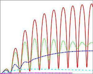
From the definition of R, it can be deduced that ${\bar{E}_0}$ is proportional to ζ ². This indicates that the contribution of streaming potential to the velocity is of O(ζ ²) in (2.17). However, if fluid elasticity dominates the flow behaviour, resonances may occur and result in a very large increase in the amplitudes of the flow rate and streaming potential (figures 6 and 7). At this time, the effect of the streaming potential field on the velocity is significant and cannot be ignored (see figure 5 for high De). As a result, the approximation (2.27) and thereby the relationship ${\bar{E}_0} \propto {R^{ - 1}}$ or ${\bar{E}_0} \propto {\zeta ^2}$ will no longer hold.

Figure 2 shows the variations of the maximum amplitude of streaming potential field, defined by ${\bar{E}_{0,max}} = \textrm{max}|{\bar{E}_0}(\omega )|$, with the ionic Péclet number ${R^{ - 1}}$ at different De. Here, the maximum amplitude occurs at the first-order resonance frequency (see figures 7a and 8b). At other frequencies, similar behaviour can also be observed. For comparison, both (2.24) and (2.27) are employed in figure 2. Using the physical properties $D = 1.9 \times {10^{ - 9}}\;{\textrm{m}^2}\;{\textrm{s}^{ - 1}}$, $\eta = 1.0 \times {10^{ - 3}}\;\textrm{kg}\;{\textrm{m}^{ - 1}}\;{\textrm{s}^{ - 1}}$, $\varepsilon = 7 \times {10^{ - 10}}\;\textrm{C}\;{\textrm{V}^{ - 1}}\;{\textrm{m}^{ - 1}}$ and ζ = 20 mV, we obtain $R \approx 7$. To extend the analysis, R is considered to range from 0.5 to 10 (equivalently, ${R^{ - 1}}$ from 0.1 to 2). We observe that when the fluid viscosity dominates the flow behaviour (represented by low De), the variations of the streaming potential given by the two equations (2.24) and (2.27) are consistent, and a linear relationship, ${\bar{E}_{0,max}} \propto {R^{ - 1}}$, can be invoked as expected. However, the approximation (2.27) gradually fails with increasing De due to the occurrence of elastic resonance and significant deviations from the linear relationship can be observed in the streaming potential field (the resonance behaviour is analysed in detail in § 3).

Figure 2. Scaling relations between the dimensionless streaming potential field and the ionic Péclet number ${R^{ - 1}}$ at different Deborah number, where ${\bar{E}_{0,max}} = \textrm{max}|{\bar{E}_0}(\omega )|$ with ${\bar{E}_0}$ provided by (2.24) (solid line) and the approximation (2.27) (dashed line). (a) K = 15, X = 0; (b) K = 5, X = 0.1.

In figure 3, we show the scaling relations between the streaming potential field ${\bar{E}_{0,max}}$ and the dimensionless EDL thickness ${K^{ - 1}}$ at different De. For viscous fluids (low De), there exist two distinct scaling regimes. For ${K^{ - 1}} < 1$, ${\bar{E}_{0,max}}$ increases with ${K^{ - 1}}$ at ${\bar{E}_{0,max}}\sim {K^{ - 2}}$, which is termed the quadratic regime by Das et al. (Reference Das, Guha and Mitra2013). For ${K^{ - 1}} > 1$, i.e. large EDL thickness relative to the channel size, ${\bar{E}_{0,max}}$ is saturated and shows no further variation with ${K^{ - 1}}$. Hence, this regime is called the saturation regime (Das et al. Reference Das, Guha and Mitra2013). When the elasticity of fluid is dominant (represented by high De, e.g. De = 10), a new regime, in addition to the above two, is observed. This regime occurs near ${K^{ - 1}} \approx 1$ (the onset of EDL overlap) and does not appear in the case of viscous fluids (see the dashed line in figure 3). In this third regime, ${\bar{E}_{0,max}}$ increases with ${K^{ - 1}}$ at ${\bar{E}_{0,max}}\sim {K^{ - 1}}$. It is called the linear regime.

Figure 3. Scaling relations between the dimensionless streaming potential field and EDL thickness ${K^{ - 1}}$ at different Deborah number, where ${\bar{E}_{0,max}} = \textrm{max}|{\bar{E}_0}(\omega )|$ with ${\bar{E}_0}$ provided by (2.24) (solid line) and the approximation (2.27) (dashed line). (a) R = 5, X = 0; (b) R = 1, X = 0.1.

2.4. Electrokinetic energy conversion

Now, consider such a fluid system connected to an external load (with resistance ${R_L}$). Due to the establishment of streaming current and potential, the mechanical energy is converted into electric energy through the external load. This fluid system can be treated as a battery with an ideal current source plus an internal resistance ${R_{ch}}$, and an equivalent circuit has been presented (see, e.g. van der Heyden et al. Reference Van der Heyden, Bonthuis, Stein, Meyer and Dekker2007). The streaming current $({I_s})$ is the current that passes through the circuit when the external resistance ${R_L}$ is zero, i.e. ${I_s}$ can be viewed as the short-circuit current in a circuit where the voltage $\Delta \phi $ is zero. The streaming potential $(\Delta {\phi _s})$ is equal to the voltage on ${R_L}$ when the value of ${R_L}$ is infinite, i.e. $\Delta {\phi _s}$ can be viewed as an open-circuit voltage in a circuit where the current I is zero. For a circuit, the instantaneous output power ${W_{out}} = I\Delta \phi $, where I is the current through ${R_L}$ and $\Delta \phi $ is the voltage across ${R_L}$. Maximum power transfer occurs at ${R_L} = {R_{ch}}$ (Olthuis et al. Reference Olthuis, Schippers, Eijkel and van den Berg2005; van der Heyden et al. Reference Van der Heyden, Bonthuis, Stein, Meyer and Dekker2007). In that case, the current through the external load is half of the streaming current, i.e. $I = {I_s}/2$, and the voltage across ${R_L}$ is half of the streaming potential, i.e. $\Delta \phi = \Delta {\phi _s}/2$. Note that in our system, the current and voltage vary with time. The time-averaged maximum output power over a cycle can be expressed as follows:

(2.28)\begin{equation}{W_{out,max}} = \frac{1}{4}\langle {I_s}\varDelta {\phi _s}\rangle = \frac{\omega }{{8{\rm \pi}}}\int_0^{2{\rm \pi}/\omega } {{I_s}(t)\varDelta {\phi _s}(t)\,\textrm{d}t} .\end{equation}

With the complex forms ${I_s}(t) = \textrm{Re}({I_{s0}}\,{\textrm{e}^{\textrm{i}\omega t}}) = ({I_{s0}}\,{\textrm{e}^{\textrm{i}\omega t}} + I_{s0}^\ast \,{\textrm{e}^{ - \textrm{i}\omega t}})/2$ and ${E_s}(t) = \textrm{Re}({E_0}\,{\textrm{e}^{\textrm{i}\omega t}}) = ({E_0}\,{\textrm{e}^{\textrm{i}\omega t}} + E_0^\ast \,{\textrm{e}^{ - \textrm{i}\omega t}})/2$ (* indicating complex conjugate), the expression $\Delta {\phi _s}(t) ={-} l{E_s}(t)$ with length l of the channel and ${I_{s0}} ={-} {I_{c0}} ={-} 2h{\sigma _b}{E_0}$, we obtain

(2.29)\begin{equation}{W_{out,max}} = \tfrac{1}{4}hl{\sigma _b}|{E_0}{|^2}.\end{equation}

With the flow rate $Q = \textrm{Re}({Q_0}\,{\textrm{e}^{\textrm{i}\omega t}})$ through the channel under a pressure difference $\Delta p = l\partial p/\partial x = l\textrm{Re}(\textrm{d}{p_0}/\textrm{d}\kern0.7pt x\,\textrm{exp(i}\omega t\textrm{)})$, the time-averaged hydrodynamic power is given by

(2.30)\begin{equation}{W_{in}} = \langle Q( - \varDelta p)\rangle ={-} \frac{l}{2}\frac{{\textrm{d}{p_0}}}{{\textrm{d}\kern0.7pt x}}\textrm{Re} ({Q_0}).\end{equation}

Note that the negative sign in the above expression is because the direction of fluid flow is consistent with that of pressure reduction. Furthermore, from (2.29), (2.30) and the non-dimensional forms (2.14) and (2.18), the efficiency of the maximum power transfer can be calculated:

(2.31a)\begin{equation}\xi = \frac{{{W_{out,max}}}}{{{W_{in}}}} = \frac{{R{K^2}|{{\bar{E}}_0}{|^2}}}{{2\textrm{Re} ({{\bar{Q}}_0})}}.\end{equation}

It is worth noting that maximum EKEC efficiency has been defined and calculated in different ways in the literature. For example, Xuan & Li (Reference Xuan and Li2006) calculated the maximum conversion efficiency based on thermodynamics, whereas van der Heyden et al. (Reference Van der Heyden, Bonthuis, Stein, Meyer and Dekker2006) calculated it based on the circuit. A few researchers (Chanda et al. Reference Chanda, Sinha and Das2014; Buren et al. Reference Buren, Jian, Zhao and Chang2018; Koranlou, Ashrafizadeh & Sadeghi Reference Koranlou, Ashrafizadeh and Sadeghi2019) defined the efficiency ξ in terms of a purely pressure-driven volume flow rate without the retardation induced by the back electro-osmotic transport.

In our recent study (Ding et al. Reference Ding, Jian and Tan2019), we demonstrated the equivalence of thermodynamic and electric circuit analyses for calculating the maximum conversion efficiency in the linear response regime. Here, the calculation of maximum EKEC efficiency based on the circuit is adopted. For comparison, we also express the maximum EKEC efficiency based on the purely pressure-driven flow rate as follows:

(2.31b)\begin{equation}\xi ^{\prime} = \frac{1}{4}\frac{{\langle {I_s}\varDelta {\phi _s}\rangle }}{{\langle {Q_p}( - \varDelta p)\rangle }} = \frac{{R{K^2}|{{\bar{E}}_0}{|^2}}}{{2\textrm{Re} ({{\bar{Q}}_{p0}})}},\end{equation}

where

(2.32)\begin{equation}{\bar{Q}_{p0}} = \frac{{2De}}{{\textrm{i}\bar{\omega }}}\left[ {1 - \frac{{\tan (\alpha )}}{\alpha }} \right]\end{equation}

is the purely pressure-driven dimensionless flow rate (see also (2.18)).

For viscous fluids, because the effect of induced streaming potential on velocity is negligible compared with the effect of pressure gradient, ${\bar{Q}_0} \approx {\bar{Q}_{p0}}$. Thus, the efficiencies calculated using (2.31a) and (2.31b) are approximately equal (Olthuis et al. Reference Olthuis, Schippers, Eijkel and van den Berg2005; Berli Reference Berli2010; Ding et al. Reference Ding, Jian and Tan2019). For viscoelastic fluids with resonance behaviour, the effect of streaming potential on the velocity cannot be ignored, and these two different definitions of EKEC efficiency result in significant differences. In particular, when (2.31b) is employed to calculate the EKEC efficiency, it predicts (incorrectly) maximum efficiency above 100 % (see figure 4), which violates the law of thermodynamics. This implies that the conversion efficiency defined by the purely pressure-driven flow rate does not apply to this condition.

Figure 4. EKEC efficiencies calculated by different definitions for Maxwell fluids (X = 0) at different De, where (a) the definition (2.31a) is used and (b) the definition (2.31b) with purely pressure-driven volume flow rate is used. Note that the meaning of the abscissa 2h/λ ₀ can be found in § 3.

3.1. Single-mode Maxwell and Oldroyd-B fluids

To facilitate the analysis of the role of elasticity, we first investigate the resonance phenomenon in electrokinetic transport based on single-mode Maxwell and Oldroyd-B fluids. Such analyses are useful in the investigation of multimode viscoelastic fluids.

In these special cases, the wavelength and damping length of the transverse waves reduce to

(3.12)\begin{equation}\frac{{{\lambda _0}}}{{2{\rm \pi}}} = \sqrt {\frac{{2{h^2}De}}{{\bar{\omega }}}} \sqrt {\frac{{1 + {X^2}{{\bar{\omega }}^2}}}{{(1 - X)\bar{\omega } + \sqrt {(1 + {{\bar{\omega }}^2})(1 + {X^2}{{\bar{\omega }}^2})} }}}\end{equation}

and

(3.13)\begin{equation}{x_0} = \sqrt {\frac{{2{h^2}De}}{{\bar{\omega }}}} \sqrt {\frac{{1 + {X^2}{{\bar{\omega }}^2}}}{{(X - 1)\bar{\omega } + \sqrt {(1 + {{\bar{\omega }}^2})(1 + {X^2}{{\bar{\omega }}^2})} }}} ,\end{equation}

which reproduce the results of Casanellas & Ortín (Reference Casanellas and Ortín2011) for Oldroyd-B fluids (note the differences in the definitions and symbols of the dimensionless variables used). The viscoelastic Stokes parameter can be rewritten in terms of De, non-dimensional frequency $\bar{\omega }$ and solvent viscosity fraction X as follows:

(3.14)\begin{equation}{\varLambda _{ve}} = \frac{1}{{\sqrt {De} }}f(\bar{\omega },X),\end{equation}

with

(3.15)\begin{equation}f(\bar{\omega },X) = \sqrt {\frac{{(X - 1){{\bar{\omega }}^2} + \bar{\omega }\sqrt {(1 + {{\bar{\omega }}^2})(1 + {X^2}{{\bar{\omega }}^2})} }}{{2(1 + {X^2}{{\bar{\omega }}^2})}}} .\end{equation}

Particularly, for Maxwell fluids (X = 0), we have

(3.16)\begin{equation}|\,f(\bar{\omega },X = 0)|= \sqrt {\frac{{\bar{\omega }\sqrt {(1 + {{\bar{\omega }}^2})} - {{\bar{\omega }}^2}}}{2}} = \sqrt {\frac{{\bar{\omega }}}{{2(\sqrt {(1 + {{\bar{\omega }}^2})} + \bar{\omega })}}} \le \frac{1}{2}\end{equation}

and

(3.17)\begin{equation}f(\bar{\omega },X = 0) \approx {\textstyle{1 \over 2}}\;\textrm{as}\;\bar{\omega } \gg 1.\end{equation}

As described by the Maxwell model, viscoelastic fluids have different flow regimes depending on the value of De (de Haro, del Río & Whitaker Reference De Haro, Del Río and Whitaker1996; del Río et al. Reference Del Río, De Haro and Whitaker1998). A critical value, De_c = 1/11.64, which determines whether a dissipative behaviour prevails or a resonance appears at a given frequency, was obtained by de Haro et al. (Reference De Haro, Del Río and Whitaker1996) through numerical calculations for permeability in porous media. In this paper, we derive a different critical value of De from a physical point of view within parallel plate geometry. Based on the viscoelastic Stokes parameter (3.14) and the accurate bound (3.16), we deduce that

(3.18)\begin{equation}{\varLambda _{ve}} = \frac{h}{{{x_0}}} < 1\quad \Leftrightarrow \quad De > \frac{1}{4}\end{equation}

for any $\bar{\omega }$ in the case of Maxwell fluids. Thus, the critical Deborah number can be obtained as De_c = 1/4. For small De (De < De_c), the damping length is small relative to the half-height of the channel and the conventional viscous effect dominates. However, beyond this critical value, the damping length is large relative to the half-height and the fluid system exhibits viscoelastic behaviour. These two flow regimes correspond to ‘wide’ and ‘narrow’ systems, respectively.

To gain some insight into the importance of the above analysis, we present some numerical calculations in the following illustrations, where the typical values of the parameters K = 15 and R = 5 have been adopted for microchannels (see (2.25) for the definition of R). The profiles of normalised axial velocity $\bar{u}$ for Maxwell fluids at different De, with and without the streaming potential effect, are shown in figure 5. In figures 5(a) and 5(b), we show the velocity profiles that satisfy the third-order resonance condition (i.e. 2h/λ ₀ = 5/2) at two time phases, ωt = 0 and ωt = ${\rm \pi}$/2, respectively. Figures 5(c) and 5(d) correspond to the destructive interference condition, 2h/λ ₀ = 3, at the same time phases (ωt = 0 and ωt = ${\rm \pi}$/2, respectively). It can be found that for De > De_c, the elastic effect manifests and the oscillating profile is maintained from plate to plate, because of the large damping length. For larger De, the elastic effect is more significant. Furthermore, when the constructive interference condition (3.10) is satisfied simultaneously, resonance occurs and the amplitude of the velocity is greatly amplified. At resonance, the velocity is in phase with the harmonic pressure gradient, i.e. the velocity is maximum at ωt = 0 and minimum at ωt = ${\rm \pi}$/2 (figure 5a,b). Conversely, outside the resonance (figure 5c,d), the velocity is nearly in quadrature with the pressure gradient and the behaviour is reversed, i.e. the velocity is maximum at ωt = ${\rm \pi}$/2 and minimum at ωt = 0. In addition, at resonances, the presence of the streaming potential tends to decrease the magnitude of velocity, especially for large De. For example, the velocity is reduced by about 40 % at De = 10 and ωt = 0 (see figure 5a).

Figure 6 shows variations of the amplitude of the normalised flow rate at different De, where two variables are used as the horizontal axes. The appearance of elastic resonance behaviour depends on De. When De > De_c, resonance may occur at some special frequencies or values of 2h/λ ₀ (see (3.10)), whereas, for De < De_c, resonance does not occur and the flow rate amplitude drops rapidly to zero. As reported by Casanellas & Ortín (Reference Casanellas and Ortín2011), the advantage of the choice of 2h/λ ₀ instead of the non-dimensional frequency $\bar{\omega }$, for the horizontal axis, is to make the location of the resonant peaks universal (independent of the fluid parameters and set-up dimensions). The increased frequency $\bar{\omega }$ corresponds to the reduced wavelength λ ₀ and, thus, the increased ratio 2h/λ ₀. In the following illustrations, we adopt 2h/λ ₀ instead of the frequency as the horizontal axis, unless otherwise specified. It is observed that the resonance greatly enhances flow rate (several orders of magnitude higher than that of Newtonian fluids). The occurrence of resonance and its locations can be characterised under the conditions given in (3.18) and (3.10), respectively, regardless of whether the streaming potential effect is included (figure 6b). Besides, the streaming potential effect tends to suppress the resonance behaviour and makes the flow rate vary smoothly with resonances, especially for large De.

Figure 6. Variations of the non-dimensional flow rate of Maxwell fluids at different De, where two variables are used as the horizontal axis: (a) non-dimensional frequency $\bar{\omega }$; (b) 2h/λ ₀, with (solid line) and without (dashed line) the streaming potential effect. For comparison, the flow rate for Newtonian fluids (De = 0) is also plotted in (b).

Figure 7(a) shows the variations of the magnitude of the normalised streaming potential with 2h/λ ₀ at different De. The resonance behaviour of the streaming potential can be observed, and it is determined under the conditions in (3.10) and (3.18). At resonances, the amplitude of the streaming potential is greatly amplified, and it is further enhanced as De increases. This explains why the influence of the streaming potential is more pronounced at resonances, as shown in figure 6(b). The EKEC efficiency ξ for Maxwell fluids as a function of 2h/λ ₀ is depicted in figure 7(b). The viscoelastic behaviour of fluids improves the EKEC efficiency. The resonance further amplifies the efficiency by several orders of magnitude compared with that of Newtonian fluids. Here, the maximum efficiency is up to 19 % in the range of the parameters. As shown in figures 6 and 7, as 2h/λ ₀ (or the frequency) increases, the peak values of the flow rate and streaming potential decrease. The maximum peak appears at the first-order resonance. However, this is not true for the EKEC efficiency; as the frequency increases, the peak values of the EKEC efficiency gradually increase and eventually tend to saturation (see figure 7b).

Figure 7. Resonance behaviours of (a) non-dimensional streaming potential and (b) EKEC efficiency ξ with 2h/λ ₀ for Maxwell fluids at different De.

Figures 5–7 show the elastic resonance phenomena in the electrokinetic flow of Maxwell fluids (X = 0) driven by a periodic pressure gradient for different De. Next, we investigate the effect of solvent viscosity using the Oldroyd-B fluids model with positive viscosity ratio X for a fixed De (figure 8). Note that the critical De (De_c = 1/4) derived based on the Maxwell fluids model is still applicable to the case of Oldroyd-B fluids. As shown in figure 8, the contribution of the Newtonian solvent tends to suppress the resonance behaviours of the flow rate and streaming potential in the electrokinetic flow. This is a result of viscous damping, and it has been observed in different contexts (Andrienko et al. Reference Andrienko, Siginer and Yanovsky2000; Casanellas & Ortín Reference Casanellas and Ortín2011).

Figure 8. Variations of (a) non-dimensional flow rate, (b) non-dimensional streaming potential and (c) EKEC efficiency ξ with the ratio 2h/λ ₀ for Oldroyd-B fluid (De = 10). Different lines correspond to different values of the viscosity ratio X.

In particular, the high-order resonance phenomena are extremely sensitive to the effect of solvent viscosity. For a small ratio X of Newtonian solvent viscosity to the total viscosity of the solution (e.g. X = 0.01), the peaks corresponding to the high-order resonances are dramatically reduced and even disappear completely. Note that high-order resonances occur at high frequencies for fixed channel dimensions and fluid properties. This shows that the effect of solvent viscosity is more important in the high-frequency regime. Besides, the relatively large solvent viscosity effect (e.g. X = 0.5) results in a shift in the position of the first-order resonance to a lower frequency relative to the case of X = 0, as given in (3.10). Furthermore, EKEC efficiency is dramatically reduced due to the solvent viscosity effect. For example, the maximum efficiency drops rapidly from 19 % to 6 % when X increases from 0 to 0.01 at a fixed De of 10 (figure 8c). In electrokinetic flows of actual viscoelastic fluids (e.g. polymer solutions), the effect of the Newtonian solvent is inevitable (Yesilata et al. Reference Yesilata, Clasen and Mckinley2006). Hence, in practice, it is almost impossible to achieve the high efficiency predicted by Bandopadhyay & Chakraborty (Reference Bandopadhyay and Chakraborty2012) and Nguyen et al. (Reference Nguyen, Van Den Meer, Van Den Berg and Eijkel2017), although utilising the resonance behaviour of viscoelastic fluids can improve the energy conversion efficiency to some extent.

3.2. Multimode viscoelastic fluids

As explained in the Introduction section, using a multimode model allows a more realistic description of fluid memory by a spectrum of relaxation times. We consider the electrokinetic transport of multimode viscoelastic fluids with the constitutive equation (1.1). This model contains the constants ${\lambda _k}$ and ${\eta _k}$ (k = 1, …, N). We adopt the convention ${\lambda _1} > {\lambda _2} > {\lambda _3} \ldots $, and to reduce the total number of parameters, we employ the following expressions to generate the relaxation time and viscosity of each mode (Bird et al. Reference Bird, Armstrong and Hassager1987):

(3.19a,b)\begin{equation}{\lambda _k} = \frac{\lambda }{{{k^\beta }}},\quad {\eta _k} = {\eta _0}\frac{{{\lambda _k}}}{{\sum\limits_k {{\lambda _k}} }},\end{equation}

where ${\eta _0}$ is the zero-shear-rate viscosity, λ a time constant and β a dimensionless quantity. In our computations, we adopt β = 2, which approximates the value obtained from the Rouse molecular theory to dilute polymer solutions (Prost-Domasky & Khomami Reference Prost-Domasky and Khomami1996). Note that in this model, ${\eta _p} = \sum {\eta _k} = {\eta _0}$, ${\lambda _k}$ decreases as k increases and the largest relaxation time λ_max = λ.

Figure 9(a) shows the variations in the magnitude of the non-dimensional flow rate with 2h/λ ₀ for various N values. The peak values of resonances decrease with an increase in N. This can be attributed to the emergence of a relatively smaller relaxation time, and a role similar to that of the Newtonian solvent component is played by the smallest relaxation time for large N. As N increases, the peak values of high-order resonances dramatically reduce, and even disappear, whereas the first-order resonance behaviour can still be observed for De > De_c, although its peak value also decreases. However, unlike the solvent viscosity effect that causes a deviation in the resonance location, in the multimode case, the position of resonances is well characterised by condition (3.10), and no significant deviation occurs (see also figure 10). The dependence of the resonance behaviour of flow rate on De is displayed in figure 9(b). We observe that De_c = 1/4 derived from the single-mode Maxwell fluid model is still applicable to the multimode case. When De > De_c, resonance occurs, whereas for De < De_c, the resonance disappears and the amplitude of the flow rate drops rapidly to zero with frequency.

Figure 9. Variations of the non-dimensional flow rate for (a) different N (De = 100) and (b) different De (N = 10). Here the solvent viscosity effect is excluded (X = 0).

Figure 10. Variations of the non-dimensional streaming potential with 2h/λ ₀ for different parameters: (a) De = 100, X = 0; (b) De = 100, X = 0.01; (c) N = 30, X = 0; and (d) N = 10, X = 0.

The variations of the magnitude of the non-dimensional streaming potential and EKEC efficiency with 2h/λ ₀ for different parameters N, De and X are depicted in figures 10 and 11, respectively. Multiple relaxation times suppress the elastic resonance behaviours of the streaming potential and EKEC efficiency relative to those of single-mode Maxwell fluids. Similar to the flow rate, the occurrence of resonance in the streaming potential field is dominated by the critical Deborah number. When De < De_c, the resonance disappears and the amplitude of streaming potential field drops to zero with frequency (see figures 10c and 10d). This can be explained as follows: the largest relaxation time determines the elastic nature of the fluid; thus, the Deborah number defined based on the largest relaxation time can capture well the appearance of elastic resonance phenomena. However, in the multimode case, the occurrence of resonance for efficiency is complex. It is dominated by De and N. For small De or large N (e.g. N > 10 in figure 11), the resonance behaviour of efficiency disappears.

Figure 11. Variations of EKEC efficiency ξ with 2h/λ ₀ for multimode viscoelastic fluids at different values of N, X and De: (a) De = 10, X = 0; (b) De = 10, X = 0.01; and (c) N = 10, X = 0.01.