4.1. Amplitude evolution equations of resonant interacting waves

In order to understand the wave generation mechanism due to the triad resonance, we derive the amplitude evolution equations of the interacting wave components by means of the classical multiple-scale perturbation analysis. Since the procedure of the multiple-scale analysis for wave resonance is standard (Mei Reference Mei1985; Kirby Reference Kirby1988; Mei et al. Reference Mei, Stiassnie and Yue2005), we only outline the key procedures and intermediate results of the analysis in appendix A. For illustration, we consider a general resonant triad in the presence of a steady uniform current, which is formed by two propagating surface wave components (with wavenumbers $k_m$ and $k_n$) and one stationary bottom ripple component (with wavenumber $k_b$), under the exact resonance condition ($k_m-k_n=k_b$ and $\omega _m=\omega _n=\omega$). The total wave solution of the velocity potential for the resonant triad can be expressed in the form

(4.1)\begin{align} \phi^{(1)}(x,z,t)&=-\frac{g A_m}{\omega-k_m U} \frac{\cosh (k_m (z+h))}{\cosh (k_m h)} \left[\frac{\mathrm{i}}{2} \exp({\mathrm{i}(k_m x - \omega t)}) \right] \nonumber\\ &\quad -\frac{g A_n}{\omega-k_n U} \frac{\cosh (k_n (z+h))}{\cosh (k_n h)} \left[\frac{\mathrm{i}}{2} \exp({\mathrm{i}(k_n x - \omega t)}) \right] \nonumber\\ &\quad - Ub \frac {g \cosh(k_b z)+U^2 k_b \sinh(k_b z)} {g \sinh(k_b h)-U^2 k_b \cosh(k_b h)} \left[\frac{\mathrm{i}}{2} \exp({\mathrm{i} k_b x}) \right] +\textrm{c.c.}, \end{align}

where $A_m$ and $A_n$ are the complex amplitudes of the propagating waves. The third term on the right-hand side of (4.1) represents the velocity potential associated with the stationary wave resulting from the uniform current passing over bottom ripples. At the resonance, $A_m$ and $A_n$ have slow $x$ and slow $t$ dependences.

Through a multiple-scale perturbation analysis summarized in appendix A, we obtain the following coupled equations governing the evolution of $A_m$ and $A_n$:

(4.2)\begin{equation} \left. \begin{gathered} \frac{\partial A_m(x,t)}{\partial t}+ C_{m} \frac{\partial A_m(x,t)}{\partial x}=\mathrm{i} A_n(x,t) \mathbb{P}, \\ \frac{\partial A_n(x,t)}{\partial t}+ C_{n} \frac{\partial A_n(x,t)}{\partial x}=\mathrm{i} A_m(x,t) \mathbb{Q}, \end{gathered} \right\}\end{equation}

where the group velocities of the propagating wave components, $C_{m}$ and $C_{n}$, and the interaction coefficients $\mathbb {P}$ and $\mathbb {Q}$ are respectively given by (A26), (A27), (A28) and (A29). The two equations in (4.2) can be decoupled to yield the separate second-order partial differential equations for $A_m(x,t)$ and $A_n(x,t)$:

(4.3)\begin{equation} \left. \begin{gathered} \frac{\partial^2 A_m(x,t)}{\partial t^2}+(C_{m}+C_{n})\frac{\partial^2 A_m(x,t)}{\partial x \partial t} +C_{m}C_{n}\frac{\partial^2 A_m(x,t)}{\partial x^2}+\mathbb{P} \mathbb{Q} A_m(x,t)=0,\\ \frac{\partial^2 A_n(x,t)}{\partial t^2}+(C_{m}+C_{n})\frac{\partial^2 A_n(x,t)}{\partial x \partial t} +C_{m}C_{n}\frac{\partial^2 A_n(x,t)}{\partial x^2}+\mathbb{P} \mathbb{Q} A_n(x,t)=0. \end{gathered}\right\} \end{equation}

With proper boundary and initial conditions, we can solve the above equations to obtain the solutions of $A_m(x,t)$ and $A_n(x,t)$. It should be noted that the above equations are similar to those derived in Kirby (Reference Kirby1988), who studied the current effects on Bragg resonant reflection of surface water waves by sand bars. The specific cases addressed in Kirby (Reference Kirby1988) are associated with triads (1) and (5) with the $k_3$ or $k_4$ wave component as the incident wave and the $k_1$ component as the reflected wave. The present study focuses on the growth of unsteady waves (from small initial disturbances) in steady current interaction with bottom ripples without incident waves.

4.2. Temporal evolution

If the rippled bottom extends indefinitely in the $x$-direction, we can consider $A_m(x,t)$ and $A_n(x,t)$ to be independent of $x$. In this special case, equations (4.3) reduce to

(4.4)\begin{equation} \left. \begin{gathered} \frac{\textrm{d}^2 A_m(t)}{\textrm{d}t^2}=- \mathbb{P} \mathbb{Q} A_m (t), \\ \frac{\textrm{d}^2 A_n(t)}{\textrm{d}t^2}=- \mathbb{P} \mathbb{Q} A_n (t). \end{gathered}\right\} \end{equation}

For given initial values of $A_m(0)=A_{m0}$ and $A_n(0)=A_{n0}$, we solve (4.4) for $A_m(t)$ and $A_n(t)$ to obtain

(4.5)\begin{equation} \left. \begin{gathered} A_m(t)=\frac{1}{2} \left( A_{m0}+\frac{\mathrm{i} A_{n0} \mathbb{P}}{\gamma} \right) \textrm{e}^{\gamma t} + \frac{1}{2} \left( A_{m0}-\frac{\mathrm{i} A_{n0} \mathbb{P}}{\gamma} \right) \textrm{e}^{-\gamma t}, \\ A_n(t)=\frac{1}{2} \left( A_{n0}+\frac{\mathrm{i} A_{m0} \mathbb{Q}}{\gamma} \right) \textrm{e}^{\gamma t} + \frac{1}{2} \left( A_{n0}-\frac{\mathrm{i} A_{m0} \mathbb{Q}}{\gamma} \right) \textrm{e}^{-\gamma t}, \end{gathered}\right\} \end{equation}

where the parameter $\gamma$ is defined as

(4.6)\begin{equation} \gamma=\sqrt{-\mathbb{PQ}}\,. \end{equation}

If $\mathbb {PQ}\geqslant 0$, $\gamma$ is imaginary (or zero) so that $|A_m(t)|$ and $|A_n(t)|$ are bounded in time. If $\mathbb {PQ}<0$, $\gamma$ is positive real so that $|A_m(t)|$ and $|A_n(t)|$ can grow exponentially with time. These indicate that the steady flow over the rippled bottom is stable (unstable) to a small disturbance consisting of wave components with wavenumbers $k_m$ and $k_n$ under the condition of $\mathbb {PQ} \geqslant 0$ ($\mathbb {PQ} < 0$). For all the six resonant triads, we numerically evaluate the value of $\mathbb {PQ}$ and present the temporal stability features in table 1. The result with triad (3) is consistent with the finding of Yih (Reference Yih1976) based on the linear instability analysis. The characteristic behaviour of the present result for flow over rippled bottoms is similar to that of McHugh (Reference McHugh1986) for flow over wavy sidewalls.

Table 1. Temporal stability of steady flow over the infinitely extended horizontal rippled bottom derived based on the triad resonance.

4.3. Spatial evolution

When the bottom contains a finite-length patch of ripples, the interest is on the spatial amplitude variation of the interacting waves after long-time triad resonant interactions. This corresponds to solving for the steady-state solutions of $A_m(x,t)=A_m(x)$ and $A_n(x,t)=A_n(x)$. After removing the terms containing time derivatives in (4.3), we obtain the spatial evolution equations for $A_m(x)$ and $A_n(x)$:

(4.7)\begin{equation} \left. \begin{gathered} \frac{\textrm{d}^2 A_m(x)}{{\textrm{d} x}^2}=-\frac{\mathbb{PQ}}{C_{m} C_{n}} A_m(x), \\ \frac{\textrm{d}^2 A_n(x)}{{\textrm{d} x}^2}=-\frac{\mathbb{PQ}}{C_{m} C_{n}} A_n(x). \end{gathered}\right\} \end{equation}

With two boundary conditions for each $A_m$ and $A_n$, the above second-order differential equations can be solved to give the solutions of $A_m(x)$ and $A_n(x)$. Depending on the situation, the boundary conditions are specified in terms of the amplitude and/or the slope of the amplitude of the wave at the ends of the rippled bottom patch.

Since our interest in this work is on the generation mechanism of upstream-propagating waves by steady flow over a rippled bottom, we consider here the resonant triad with wavenumber combination (6). In this triad, the $k_1$ wave propagates upstream while the (energy of the) $k_2$ wave propagates downstream. The bottom ripples are assumed to be located within $0 \leqslant x\leqslant L$, outside of which the bottom is horizontal. For the boundary conditions, we consider that, at the downstream end of the rippled bottom patch ($x=L$), the $k_2$ wave has a small amplitude $A_2(x=L)=a_2$ and the $k_1$ wave has a negligibly small amplitude $A_1(x=L)=0$ (as the generation of the $k_1$ wave by the triad resonance starts at $x=L$). From (4.2), these amplitude boundary conditions also imply the following conditions for the slope of the amplitude: $\textrm {d}A_2/{\textrm {d} x} (x=L)=0$ and $\textrm {d}A_1/{\textrm {d} x} (x=L)=\mathrm {i} a_2 \mathbb {P}/C_{1}$. With these boundary conditions, we solve (4.7) to obtain the solution of $A_1(x)$ and $A_2(x)$ given by

(4.8a,b)\begin{equation} A_1(x)=\mathrm{i} \frac{a_2 \mathbb{P}}{\theta C_{1}}\sinh(\theta(x-L)) \quad \mbox{and}\quad A_2(x)=a_2 \cosh (\theta (x-L)), \end{equation}

where the parameter $\theta$ is defined as

(4.9)\begin{equation} \theta=\sqrt{- \frac{\mathbb{PQ}}{C_{1}C_{2}}}\,. \end{equation}

If ${\mathbb {PQ}}/{C_{1}C_{2}}\geqslant 0$, then $\theta$ is imaginary (or zero) and $A_{1,2}(x)$ are sine and/or cosine functions of $x$ whose amplitudes are bounded. If ${\mathbb {PQ}}/{C_{1}C_{2}}<0$, then $\theta$ is positive real so that $A_{1,2}(x)$ can grow exponentially in $x$. Similar results for other triads can be obtained. Table 2 presents the spatial stability features of steady flow over the infinitely extended rippled bottom associated with all the six resonant triads.

Table 2. Spatial stability of steady flow over the infinitely extended horizontal rippled bottom derived based on the triad resonance.

As a numerical illustration, we consider one of the experimental cases to be described in the next section, for which we have $L/\lambda _b=7.5$, $h/\lambda _b=0.8$ and $\epsilon _b\equiv k_b b=0.602$, where $\lambda _b=2{\rm \pi} /k_b$. For this bottom ripple configuration, figure 6 displays the values of $\mathbb {P}$, $\mathbb {Q}$, $C_{1}$ and $C_{2}$ as functions of $F_r$ for the resonant triad (6). Both $\mathbb {P}$ and $\mathbb {Q}$ are positive, and, as expected, $C_{2}$ is positive while $C_{1}$ is negative. As a result, the parameter $\theta$ is real and positive, as shown in figure 7(a). The amplitudes of the generated unsteady waves $A_{1,2}(x)$ thus achieve an exponential growth with the interaction distance $L-x$. Figure 7(b) plots the maximum amplitude of the upstream-propagating $k_1$ wave obtained at $x=0$ as a function of $F_r$, which is seen to decrease with increasing $F_r$.

Figure 6. (a) Dimensionless group velocities $C_{1}/\sqrt {gh}$ (------) and $C_{2}/\sqrt {gh}$ (- - -), and (b) dimensionless interaction coefficients $\tilde {P}=\mathbb {P}\sqrt {h/g}$ (------) and $\tilde {Q}=\mathbb {Q}\sqrt {h/g}$ (- - -) as functions of $F_r$ for resonant triad (6). (Here $L/\lambda _b=7.5$, $h/\lambda _b=0.8$ and $\epsilon _b=0.602$.)

Figure 7. (a) Spatial growth rate $\theta$ and (b) maximum amplitude of the generated upstream-propagating wave, $|A_1(0)/a_2|$, as functions of $F_r$ for resonant triad (6). (Here $L/\lambda _b=7.5$, $h/\lambda _b=0.8$, and $\epsilon _b=0.602$.)

We note that, since $\mathbb {P}\mathbb {Q}$ is always positive, the parameter $\gamma$ is pure imaginary from (4.6). In the case of bottom ripples that are uniformly extended to infinity, the unsteady wave components in the triad (6) do not grow exponentially with time. This indicates that the steady flow is temporally stable to the disturbance dominated by $k_1$ and $k_2$ wave components. On the other hand, the above results show that the steady flow is spatially unstable to the $k_1$ and $k_2$ wave disturbance. This cannot be obtained by the temporal instability analysis (Yih Reference Yih1976; Raj & Guha Reference Raj and Guha2019).

If the resonance condition is not satisfied exactly, the detuning effect should be included in the solution. For illustration, we consider the detuning case in which the frequency ($\omega$) of the generated unsteady waves is fixed while the current speed is shifted by a small amount ${\rm \Delta} U$ from the speed $U$ under the exact resonance condition ($\omega , U$). The current speed detuning ${\rm \Delta} U$ causes the wavenumber detunings ${\rm \Delta} k_1$ and ${\rm \Delta} k_2$ in $k_1$ and $k_2$, which can be calculated from the dispersion relation (with the use of $\omega$ and $U+{\rm \Delta} U$). Since $\omega$ is invariant, the evolution equations for $A_1(x)$ and $A_2(x)$ are found to take the same form as (4.7) but with the coefficients evaluated at the detuning condition (i.e. $\omega$, $U+{\rm \Delta} U$, $k_1+{\rm \Delta} k_1$, $k_2+{\rm \Delta} k_2$). Taking the exact resonance at $F_r=0.3$ (cf. figure 7b) as an example, we examine the solution of the resonance-generated upstream-propagating wave amplitude as a function of the current speed detuning ${\rm \Delta} U$. Figure 8 shows $C_{1}$, $C_{2}$, $\mathbb {P}$ and $\mathbb {Q}$ while figure 9 shows the growth rate $\theta$ and maximum amplitude of the upstream-propagating wave $|A_1(0)|$ as functions of ${\rm \Delta} U$. It is seen that $|A_1(0)|$ becomes unbounded when the detuned current speed approaches the critical speed $U_c$ (associated with the critical frequency $\omega _c=\omega$ considered). (The relation between $U_c$ and the critical wave frequency $\omega _c$ is shown in figure 2b.) The singular behaviour of $|A_1(0)|$ results from the fact that $\theta$ becomes infinitely large as both $C_{1}$ and $C_{2}$ approach zero at $U_c$. These results indicate that, despite not at the exact resonance, the generation of upstream-propagating waves is substantially amplified in the neighbourhood of the critical current speed $U_c$ (or critical frequency $\omega _c$) due to the continuous buildup of energy in time for the unsteady $k_1$ and $k_2$ waves from the near-resonant triad interaction. We remark that the exact resonance does not occur at the critical flow condition under which $k_1=k_2$, so that the triad resonance condition cannot be satisfied exactly.

Figure 8. (a) Dimensionless group velocities $C_{1}/U$ (------) and $C_{2}/U$ (- - -), and (b) dimensionless interaction coefficients $\tilde {P}=\mathbb {P}\sqrt {h/g}$ (------) and $\tilde {Q}=\mathbb {Q}\sqrt {h/g}$ (- - -) as functions of current speed detuning $\Delta U/U$ from the exact resonance of triad (6). (Here $L/\lambda _b=7.5$, $h/\lambda _b=0.8$, $F_r=0.30$ and $\epsilon _b=0.602$.) The vertical line (— $\cdot$ —) represents the critical wave-flow condition.

Figure 9. (a) Spatial growth rate $\theta$ and (b) maximum amplitude of generated upstream-propagating wave, $|A_1(0)/a_2|$, as functions of current speed detuning ${\rm \Delta} U/U$ from the exact resonance of triad (6). (Here $L/\lambda _b=7.5$, $h/\lambda _b=0.8$, $F_r=0.30$ and $\epsilon _b=0.602$.) The vertical line (— $\cdot$ —) represents the critical wave-flow condition.

5.1. Experimental apparatus and set-up

To assist in understanding the phenomenon and verify the theoretical analysis of upstream-propagating wave generation in steady flow over a rippled bottom, we conducted a series of laboratory experiments in a relatively large-scale wave flume. The experimental set-up and configurations were optimized on the basis of Kyotoh's preliminary observation of upstream-advancing waves in a rather small wave flume (Kyotoh & Fukushima Reference Kyotoh and Fukushima1997). While the design and initial stage of the experiments as well as some preliminary qualitative observations were reported in Fan et al. (Reference Fan, Zheng, Tao, Yu and Wang2016), the experimental set-up was improved and the experiments were recalibrated for better accuracy afterwards. The quantitative experimental results presented in this paper have not been reported elsewhere. For clarity and completeness, we summarize the latest primary experimental set-up, apparatus and calibrations below.

Figure 10 displays a sketch of the flume experiment set-up. Unlike in Kyotoh & Fukushima (Reference Kyotoh and Fukushima1997), where the flume bottom was inclined to produce the incoming flow, we chose to use a horizontal flume bottom with a steady incoming flow generated by a water pump installed under the flume. The longitudinal distance between the upstream flow inlet and the downstream flow outlet is 51.0 m. The width and height of the flume are 1.0 m and 1.5 m, respectively. A patch of rippled wooden bottom consisting of seven-and-a-half sinusoidal ripples was installed in the relatively downstream side of the flume. The length of the rippled patch is $L_b=1.80$ m, with the ripple wavelength equal to $\lambda _b=0.24$ m. Four different ripple amplitudes of $b=0.040$, 0.0305, 0.0265 and 0.023 m were used in the experiments. The corresponding ripple steepnesses are $\epsilon _b\equiv k_b b=2{\rm \pi} b/\lambda _b=1.047$, 0.798, 0.694 and 0.602, respectively. The centre of the rippled patch is 33.0 m away from the upstream flow inlet. The rippled patch was embedded into the flume's flat bottom so that the average water depth is nearly equal to that over the flat bottom in the flume.

Figure 10. Sketch of the flume experiment set-up.

For each rippled bottom configuration, a wide range of water depths and incoming flow velocities, as displayed in table 3, were tested to ensure the observation of upstream-propagating waves. The range of parameters considered in table 3 is mainly for intermediate and shallow depths. In order to measure the free-surface oscillation, a total of 26 capacitive wave gauges were installed along the transverse centreline of the flume, 17 of which were uniformly set above the rippled bottom with a horizontal spatial interval of 0.12 m (equal to a half of the ripple wavelength), as shown in figure 10. For measuring the upstream-propagating waves, six wave gauges were set as three pairs upstream of the rippled bottom. Their distances from the upstream edge of the rippled patch are 3.0 m, 6.0 m and 9.0 m, respectively. In each pair, the distance between the wave gauges is set to be 0.30 m in order to calculate the wavelength of the upstream-propagating waves. (Note that this distance is much less than the wavelength of the observed upstream-propagating waves.) Besides these, another pair and one single wave gauges were placed downstream at 3.75 m and 6.75 m from the downstream edge of the rippled bottom, respectively. In the experiments, the flow conditions in the flume were calibrated before each test. The relationship between flow volume and voltage of the water pump's converter was acquired and utilized to calculate the input voltage for each experimental case.

Table 3. Ranges of Froude number $F_r$ for different combinations of bottom ripple steepness and water depth that were tested with the observation of upstream-propagating waves in the experiments.

5.2. Experimental results

We observed in the experiments that, for given rippled bottom configuration and water depth, unsteady waves that propagate against the steady incoming current are generated when the current reaches a narrow critical range of speed. For the current speed outside the critical range, such unsteady wave generation was not observed. For given ripple wavenumber, the critical range of current speed for upstream-propagating wave generation varies with water depth and ripple amplitude; and the frequency of the generated upstream-propagating waves is dependent on the current speed and water depth.

Figure 11 displays sample time variations and corresponding amplitude spectra of the free-surface elevations far upstream of the rippled bottom, above the rippled bottom and downstream of the rippled bottom in the case with $\epsilon _b=0.798$, $h/\lambda _b=0.6$ and $F_r=0.280$. In the upstream location and over the rippled bottom, the free-surface elevation shows the presence of a dominant wave component at the same frequency $\omega =2{\rm \pi} f=4.75\ \textrm {rad}\ \textrm {s}^{-1}$. Downstream, the free-surface elevation is composed of small broad-banded wave components without a clear dominant component. Figure 12 shows a sample instantaneous free-surface pattern with the presence of monochromatic upstream-propagating waves.

Figure 11. Time variations (a–c) and amplitude spectra (d–f) of the free-surface elevations (a,d) at the upstream side of the rippled bottom ($x/\lambda _b=-38.125$), (b,e) above the rippled bottom ($x/\lambda _b=3.75$) and (c,f) at the downstream side of the rippled bottom ($x/\lambda _b=22.5$). (Here $h/\lambda _b=0.6$, $F_r=0.280$ and $\epsilon _b=0.798$.)

Figure 12. Instantaneous free-surface pattern upstream of the rippled bottom, showing the presence of upstream-propagating waves for the experimental case in figure 11. (b) Close-up of the enclosed region in panel (a).

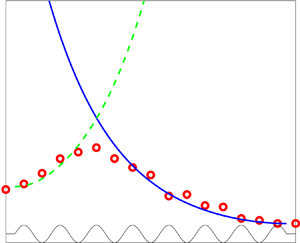
Figure 13 plots the amplitude of the dominant component of the generated upstream-propagating waves, which is measured in the upstream flat horizontal bottom, as a function of current speed for different ripple steepnesses and water depths. The data show that the upstream-propagating waves with significantly large amplitude exist only in the narrow critical range of current speed for a given ripple configuration and water depth. The amplitude of the unsteady wave is negligibly small away from the critical range of current speed. For given ripple steepness, the critical current speed is observed to increase as the water depth decreases. For given water depth, the critical current speed is seen to decrease as the ripple steepness increases. The wave generation phenomenon becomes weaker at larger water depth in general. The upper limit of water depth for the observed wave generation becomes larger with steeper bottom ripples.

Figure 13. Experimental data of the amplitude of upstream-propagating waves (over the upstream flat bottom) as a function of the Froude number ($F_r$) for the bottom ripple steepness (a) $\epsilon _b=0.602$, (b) 0.694, (c) 0.798 and (d) 1.047 with water depth $h/\lambda _b= 0.5$ ($\diamond$), 0.6 ($\square$), 0.7 ($\bigcirc$), 0.8 ($\triangle$), 0.9 ($+$) and 1.0 ($\ast$).

Figure 14 depicts the period of upstream-propagating waves as a function of current speed for different bottom steepnesses and water depths. The results indicate that the period of the upstream-propagating waves is in the narrow range of 1.2 s to 1.5 s. The wave period generally becomes larger with increasing current speed except at very shallow water depth and steep bottom ripples, under which the wave motion over the rippled area is strongly nonlinear.

Figure 14. Experimental data of the period of upstream-propagating waves (over the upstream flat bottom) as a function of the Froude number ($F_r$) for the bottom ripple steepness (a) $\epsilon _b=0.602$, (b) 0.694, (c) 0.798 and (d) 1.047 with water depth $h/\lambda _b=0.5$ ($\diamond$), 0.6 ($\square$), 0.7 ($\bigcirc$), 0.8 ($\triangle$), 0.9 ($+$) and 1.0 ($\ast$).

Figure 15 displays the spatial variation of the generated unsteady wave amplitude over the rippled bottom patch as well as upstream of the patch. In this figure, only representative cases are plotted for clarity. For all the cases shown, the unsteady wave amplitude increases rapidly from a near-zero value with distance from the downstream edge of the rippled bottom and reaches a peak value at approximately one to two ripple wavelengths from the upstream edge of the rippled bottom, and then reduces to a near-constant value over the flat upstream bottom. The unsteady wave amplitude is seen to be negligibly small over the downstream flat bottom.

Figure 15. Experimental data of the spatial variation of the unsteady wave amplitude over the rippled bottom and upstream flat bottom with: (a) $\epsilon _b=0.602$ for $h/\lambda _b=0.5$ and $F_r=0.320$ ($\diamond$), $h/\lambda _b=0.6$ and $F_r=0.315$ ($\square$), $h/\lambda _b=0.7$ and $F_r=0.305$ ($\bigcirc$) and $h/\lambda _b=0.8$ and $F_r=0.300$ ($\triangle$); (b) $\epsilon _b=0.694$ for $h/\lambda _b=0.5$ and $F_r=0.300$ ($\diamond$), $h/\lambda _b=0.6$ and $F_r=0.305$ ($\square$), $h/\lambda _b=0.7$ and $F_r=0.285$ ($\bigcirc$) and $h/\lambda _b=0.8$ and $F_r=0.285$ ($\triangle$); (c) $\epsilon _b=0.798$ for $h/\lambda _b=0.6$ and $F_r=0.280$ ($\square$), $h/\lambda _b=0.7$ and $F_r=0.275$ ($\bigcirc$) and $h/\lambda _b=0.8$ and $F_r=0.270$ ($\triangle$); and (d) $\epsilon _b=1.047$ for $h/\lambda _b=0.6$ and $F_r=0.250$ ($\square$), $h/\lambda _b=0.7$ and $F_r=0.240$ ($\bigcirc$), $h/\lambda _b=0.8$ and $F_r=0.240$ ($\triangle$) and $h/\lambda _b=0.9$ and $F_r=0.230$ ($+$). (Note that the horizontal scale over the flat bottom for $x<0$ differs from that over the rippled bottom for $x\geqslant 0$.)

Apart from the wave amplitude, we show in figure 16 the spatial variation of the primary unsteady wave period over the rippled bottom patch for some representative cases. The experimental data indicates that the periods of the generated (dominant) unsteady wave components in all cases remain nearly invariant over the entire rippled bottom. We note that, in the case of very shallow depth and steep ripples, super-harmonic (double-frequency) wave components are also observed due to strong nonlinear free-surface boundary effects.

Figure 16. Experimental data of the spatial variation of the primary unsteady wave period over the rippled bottom with: $\epsilon _b=0.602$, $h/\lambda _b=0.5$ and $F_r=0.320$ ($\diamond$); $\epsilon _b=0.694$, $h/\lambda _b=0.6$ and $F_r=0.305$ ($\square$); $\epsilon _b=0.798$, $h/\lambda _b=0.7$ and $F_r=0.275$ ($\bigcirc$); and $\epsilon _b=1.047$, $h/\lambda _b=0.9$ and $F_r=0.230$ ($+$).

6.1. Period of generated upstream-propagating wave versus current speed

As discussed in § 3, resonant triads (1), (5) and (6) all involve the upstream-propagating ($k_1$) wave component. Among them, triad (5) can be excluded since the steady flow is spatially stable to small unsteady wave disturbances that are contained in triad (5) (see table 2). In principle, triads (1) and (6) could produce the $k_1$ wave component. The experimental data of the observed $k_1$ wave period, however, clearly exclude the possible participation of triad (1). We thus compare the theory with experiments for triad (6) only.

We first compare the frequency and wavenumber of the unsteady wave measured at the upstream side of the rippled bottom patch in the flume with the theoretical prediction from the resonance condition of triad (6). For the experimental data, the wave frequency is chosen to be the peak frequency of the free-surface elevation spectrum. The wavenumber is calculated from its relation with the frequency and phase speed. The phase speed of the wave can be determined from the correlation coefficient of the wave elevation measured at two neighbouring wave gauges (Kyotoh & Fukushima Reference Kyotoh and Fukushima1997).

In figures 17–21, we present the experimental data of the frequency of the observed upstream-propagating waves versus the associated incoming current speed with different ripple steepnesses and water depths. In relatively deep depth ($h/\lambda _b=0.9$), the data for the mildest ripple case ($\epsilon _b=0.602$) are not shown in figure 17 since the amplitude of the upstream-propagating wave is negligibly small. In the shallow depth ($h/\lambda _b=0.5$), the data for the steep ripple cases ($\epsilon _b=0.798$ and 1.047) are not shown in figure 21 since the flow motion is strongly nonlinear and turbulent. In these figures, the theoretical condition for the resonant triad (6), expressed as the relation between the frequency of the upstream-propagating wave and the incoming current speed, is also shown for comparison with the experimental data. The comparisons show that, in the cases with relatively mild ripples and large water depths, the experimental data fall right on or very close to the theoretical curves. In the cases with steeper ripples and shallow water depths, the experimental data somewhat shift from the theoretical curves to the lower current speeds. The discrepancy between the experimental data and the theoretical prediction becomes larger as the ripple steepness increases and/or water depth decreases. We note that the theory assumes a uniform incoming current while the experimental data use the average flow velocity, which is equal to the flow flux divided by the mean water depth over the flat bottom. Owing to the real-fluid effect in the experiments, the flow velocity near the free surface is known to be larger in magnitude than the average velocity. This effect is stronger for shallower depth. After taking this fact into account, the experimental data would move towards larger current speeds, leading to better agreement with the theory than appeared in figures 17–21.

Figure 17. Comparison of the frequency ($\varOmega =\omega (h/g)^{1/2}$) of the triad-resonance-generated upstream-propagating wave as a function of current speed ($F_r=U/(gh)^{1/2}$) between the experimental measurements ($\square$) and the theoretical prediction from the resonance condition for triad (6) (------) in the case of water depth $h/\lambda _b=0.9$ and bottom ripple steepness (a) $\epsilon _b=0.694$, (b) 0.798 and (c) 1.047. The critical flow condition over the rippled bottom region (- - -) is shown for reference.

Figure 18. Comparison of the frequency ($\varOmega =\omega (h/g)^{1/2}$) of the triad-resonance-generated upstream-propagating wave as a function of current speed ($F_r=U/(gh)^{1/2}$) between the experimental measurements ($\square$) and the theoretical prediction from the resonance condition for triad (6) (------) in the case of water depth $h/\lambda _b=0.8$ and bottom ripple steepness (a) $\epsilon _b=0.602$, (b) 0.694, (c) 0.798 and (d) 1.047. The critical flow condition over the rippled bottom region (- - -) is shown for reference.

Figure 19. Comparison of the frequency ($\varOmega =\omega (h/g)^{1/2}$) of the triad-resonance-generated upstream-propagating wave as a function of current speed ($F_r=U/(gh)^{1/2}$) between the experimental measurements ($\square$) and the theoretical prediction from the resonance condition for triad (6) (------) in the case of water depth $h/\lambda _b=0.7$ and bottom ripple steepness (a) $\epsilon _b=0.602$, (b) 0.694, (c) 0.798 and (d) 1.047. The critical flow condition over the rippled bottom region (- - -) is shown for reference.

Figure 20. Comparison of the frequency ($\varOmega =\omega (h/g)^{1/2}$) of the triad-resonance-generated upstream-propagating wave as a function of current speed ($F_r=U/(gh)^{1/2}$) between the experimental measurements ($\square$) and the theoretical prediction from the resonance condition for triad (6) (------) in the case of water depth $h/\lambda _b=0.6$ and bottom ripple steepness (a) $\epsilon _b=0.602$, (b) 0.694, (c) 0.798 and (d) 1.047. The critical flow condition over the rippled bottom region (- - -) is shown for reference.

Figure 21. Comparison of the frequency ($\varOmega =\omega (h/g)^{1/2}$) of the triad-resonance-generated upstream-propagating wave as a function of current speed ($F_r=U/(gh)^{1/2}$) between the experimental measurements ($\square$) and the theoretical prediction from the resonance condition for triad (6) (------) in the case of water depth $h/\lambda _b=0.5$ and bottom ripple steepness (a) $\epsilon _b=0.602$ and (b) 0.694. The critical flow condition over the rippled bottom region (- - -) is shown for reference.

Figure 22 shows the comparisons of the wavenumber of the upstream-propagating waves as a function of the current speed between the experimental measurements and the theoretical prediction from the resonance condition for triad (6). Consistent with the frequency comparisons shown in figures 17–21, better agreements between the experimental data and the theoretical prediction are obtained for the cases with mild bottom ripples and/or relatively large water depths. As discussed above, if the real-fluid effect on the surface current speed is accounted for, the experimental data in the cases of steep bottom ripples and shallow water depth would be moved to larger values of $F_r$, leading to better agreements with the theory.

Figure 22. Comparison of the wavenumber ($k_1h$) of the triad-resonance-generated upstream-propagating wave as a function of current speed ($F_r=U/(gh)^{1/2}$) between the theoretical prediction from the resonance condition for triad (6) (------) and the experimental measurements with bottom ripple steepness $\epsilon _b=0.602$ ($\square$), 0.694 ($\ast$), 0.798 ($\bigcirc$) and 1.047 ($\bigtriangleup$) and water depth (a) $h/\lambda _b=0.9$, (b) 0.8, (c) 0.7, (d) 0.6 and (e) 0.5.

The good agreements between the experimental data and the theory on the kinematics of the upstream-propagating waves confirm that the triad resonance involving the unsteady $k_1$ and $k_2$ waves as well as stationary bottom ripples (and/or the resulting steady waves) is capable of producing upstream-propagating waves (i.e. with wavenumber $k_1$) when a steady current passes over a rippled bottom patch. The remaining question is why the generation of upstream-propagating waves in the experiment is clearly observed only in a narrow range of current speeds but not for speeds outside this critical range, for which the same type of triad resonances can also occur in theory.

The analysis in § 4.3 indicates that the amplitude of the upstream-propagating wave can be significantly amplified if the triad resonance happens in the neighbourhood of the critical wave-flow condition (described in terms of critical current speed $U_c$ and critical wave frequency $\omega _c$). Note that $\omega _c$ is uniquely related to $U_c$ as shown in figure 2(b). To examine the role of the critical wave flow on the upstream-propagating wave generation in the experiments, we need to estimate the (near-surface) current speed over the rippled bottom patch where the triad resonant wave–ripple interactions occur. The average current speed over the rippled bottom patch ($\tilde {U}$) is actually larger than the ideal uniform current speed ($U$) (used in the theoretical analysis) due to two factors associated with the real-fluid effects in the flow over bottom ripples.

First, it is known from the existing numerical and experimental studies in the literature that, when a uniform incoming flow passes over a sinusoidal rippled solid surface, flow separation occurs in the case of relatively large ripple amplitudes (Zilker & Hanratty Reference Zilker and Hanratty1979; Buckles, Hanratty & Adrian Reference Buckles, Hanratty and Adrian1984; Kuzan, Hanratty & Adrian Reference Kuzan, Hanratty and Adrian1989; Hudson, Dykhno & Hanratty Reference Hudson, Dykhno and Hanratty1996; Shen et al. Reference Shen, Zhang, Yue and Triantafyllou2003). Since the time-averaged flow velocity in the separated-flow region on the leeward side of ripples is much smaller than outside the separated-flow region (Buckles et al. Reference Buckles, Hanratty and Adrian1984), it is reasonable (and in fact conservative) to assume that the effective depth over which the flow fluxes downstream is the distance from the crest of the ripples to the mean water surface, $h-b$. This would enlarge $\tilde {U}$ from $U$ by a factor of $\xi _1=h/(h-b)$.

Second, the incoming current in the flume is actually a shear flow over the stationary flat bottom so that the flow velocity near the free surface is larger than the depth-averaged speed $U$. Figure 23 shows the experimental data of two sample vertical profiles of steady current in the flume of a flat bottom. The approximate velocity profiles from the empirical $1/7\textrm {th}$ and $1/11\textrm {th}$ power laws for the fully developed boundary layers are also shown for comparison. At relatively large water depth with smaller velocity, the velocity profile is seen to match the $1/7\textrm {th}$ power law well. At shallow depth with larger velocity, the velocity profile is better described by the $1/n\textrm {th}$ power law with $n>7$, which is consistent with the finding in the literature (Schlichting & Gersten Reference Schlichting and Gersten2017). For illustration, based on the empirical $1/7\textrm {th}$ power law (White Reference White2006), we obtain the displacement thickness $\delta ^*=h/8$. This effect would further enlarge $\tilde {U}$ from $U$ by a factor of $\xi _2=h/(h-\delta ^*)=1.143$. Upon combining these two real-fluid effects, we have the relation $\tilde {U} =\xi _1\xi _2 U$.

Figure 23. Vertical profiles of horizontal velocity of the steady current in the flume with a flat bottom with water depth (a) $h/\lambda _b=0.9$ and (b) 0.6, where $\lambda _b=0.24$ m. The symbols and curves represent the experimental data from velocity gauges A ($\bigtriangleup$), B ($\square$) and C ($\bigcirc$) as well as the approximate velocity profiles from the $1/7\textrm {th}$ (------) and $1/11\textrm {th}$ ($\cdots \cdots$) power laws. (Gauges A, B and C are located at 1.5 m, 0.9 m and 0.3 m from the upstream edge of the ripple patch.)

In figures 17–21, we plot the critical wave-flow condition over the rippled bottom patch, which is represented by the dashed line. We note that the theoretical resonance condition for triad (6) and the experimental data points in these figures are displayed in terms of the ideal (depth-averaged) uniform current velocity $U$ (i.e. $F_r=U/(gh)^{1/2}$). Thus, any point on this dashed line represents that the wave flow over the rippled bottom has the critical wave frequency ($\omega _c$) and critical current speed ${\tilde {U}}_c$, while the corresponding uniform flow speed over the flat bottom is given by $U={\tilde {U}}_c/(\xi _1\xi _2)$. We see in figures 17–21 that the experimental data points are clustered in the close neighbourhood of the intersection of the critical wave-flow curve and the triad resonance condition curve. In particular, the experimental data points are seen to be right at this intersection point in the cases with mild ripples and large water depths. This shows that the observable upstream-propagating waves (with a significantly large amplitude) are generated by the triad resonant wave–ripple interactions only when the wave flow over the rippled bottom region is near the critical condition associated with wave frequency $\omega _c$ and current speed ${\tilde U}_c$. For steeper ripples at shallower water depth, the experimental data points are seen to slightly deviate from this intersection point to lower current speed. This deviation may be due to several factors. First, as mentioned above, since the experimental data points are plotted in terms of the uniform depth-averaged flow speed $U$, they are shifted to somewhat lower speed due to the shear flow effect. Second, the flow separation effect near the rippled bottom is underestimated by the use of $\xi _1$, especially at relatively shallow depth and steeper ripples. Third, nonlinear ripple amplitude effects on the wave dispersion relation could influence the theoretical prediction of the triad resonance condition (which is based on the linear dispersion relation in the present study). Detailed understanding and quantification of these real-fluid and higher-order nonlinear effects requires the use of expensive turbulent flow computations, which is beyond the scope of this work.

Away from the neighbourhood of the intersection point, the triad resonant wave–ripple interaction still occurs, but with the growth rate $\theta =O(1)$ (i.e. bounded). In this case, as the analysis in § 4.3 shows, the maximum amplitude of the generated upstream-propagating wave depends on the length ($L$) of the rippled bottom patch. As a result, the generated upstream-propagating waves may not be observable in the physical experiments if $L$ is not sufficiently large. This is consistent with the feature of comparisons between the experiment and the present theory in figures 17–21.

6.2. Spatial variation of upstream-propagating wave amplitude

The theoretical analysis in § 4.3 provides an asymptotic solution of the amplitudes, (4.8a,b), of the interacting waves involved in the triad resonance or near-resonance. For given bottom ripple properties and water depth, the current speed ($\tilde {U}$) over the rippled bottom patch and the amplitude of the $k_2$ wave ($a_2$) at the starting location ($x=L$) of resonant wave–ripple interactions are needed to evaluate the theoretical solution of $A_1(x)$ and $A_2(x)$. To compare the theoretical prediction with the experimental measurements, we let $a_2$ be the small experimental value of the unsteady wave amplitude at $x=L$. To determine $\tilde {U}$, we match the theoretical solution of the (maximum) unsteady wave amplitude $|A_1(x)+A_2(x)|$ to the experimental data.

Figure 24 displays representative comparisons of the theoretical solution of $|A_1(x)+A_2(x)|$, given by (4.8a,b), with the experimental data for two sample cases with (a) $\epsilon _b=0.602$, $h/\lambda _b=0.8$ and $F_r=0.30$ and (b) $\epsilon _b=0.694$, $h/\lambda _b=0.7$ and $F_r=0.285$, respectively. For the theoretical solution, $\tilde {U}=0.994U_c$ and $\tilde {U}=0.985U_c$ are used in cases (a) and (b), respectively. It is seen that the theoretical prediction agrees with the experimental data very well over most of the rippled bottom patch (for $(2\text {--}2.5)\lambda _b \leqslant x \leqslant L$), in particular, on the feature of exponential growth of $A_{1,2}(x)$ with the interaction distance from the starting point ($L-x$). In the upstream end region of the rippled patch ($0 \leqslant x < (2\text {--}2.5)\lambda _b$), unlike the theoretical solution, the experimental data show that $|A_1(x)+A_2(x)|$ reverses the trend of exponential growth with $L-x$ and reduces to a value that matches the amplitude of upstream-propagating waves over the flat bottom. The reason for the deviation of the experimental data from the theoretical prediction (4.8a,b) is that, in the experiment, the current speed $U$ over the upstream flat bottom is slightly smaller than $\tilde {U}$ over the rippled patch so that $A_2$ must decrease to vanish at $x=0$ since the $k_2$ wave cannot exist in the upstream flat bottom. This would reduce the growth of $A_1(x)$ by the triad resonance in the region near the upstream end of the rippled bottom patch. This effect is, however, not considered in the theoretical solution (4.8a,b), which is determined based on the boundary conditions at the downstream end only.

Figure 24. Comparison of the amplitude of unsteady waves, $|A_1(x)+A_2(x)|$, over the rippled bottom patch between the experimental measurement ($\bigcirc$) and the theoretical solutions (4.8a,b) (------) and (6.1a,b) (- - -) for: (a) $\epsilon _b=0.602$, $h/\lambda _b=0.8$ and $F_r=0.30$; and (b) $\epsilon _b=0.694$, $h/\lambda _b=0.7$ and $F_r=0.285$.

While it is an uneasy analytical practice to derive the theoretical solution that accounts for the varying current speed effect over the entire rippled bottom patch, we can obtain an asymptotic solution in the upstream end region of the rippled patch, which is controlled by the boundary conditions at $x=0$. We consider the boundary conditions: $A_2(x=0)=0$ and $A_1(x=0)=a_1$, with $a_1$ being equal to the experimental measurement of the unsteady wave amplitude at $x=0$. From (4.2), we obtain the slope condition: $\textrm {d}A_1/{\textrm {d} x} (x=0)=0$ and $\textrm {d}A_2/{\textrm {d} x} (x=0)=\mathrm {i} a_1 \mathbb {Q}/C_{2}$. With these boundary conditions, we solve (4.7) for $A_1(x)$ and $A_2(x)$ to obtain:

(6.1a,b)\begin{equation} A_1(x)=a_1 \cosh (\theta x) \quad \mbox{and}\quad A_2(x)=\mathrm{i} a_1 \frac{\mathbb{Q}}{\theta C_{2}}\sinh(\theta x). \end{equation}

For comparison, these solutions (with $\tilde {U}=0.994U_c$ and $0.985U_c$, respectively, for cases (a) and (b)) are also presented in figure 24. It is seen that the theoretical solution (6.1a,b) matches the experimental data quite well in the upstream end region of the rippled patch ($0 \leqslant x < (1.5\text {--}2) \lambda _b$). Together, the theoretical solutions (4.8a,b) and (6.1a,b) properly reflect the distinctive growth feature of the unsteady waves by near-triad resonance over the rippled bottom patch observed in the experiment. In addition, the results of $\tilde {U}=0.994U_c$ and $0.985U_c$ in these two sample cases further confirm that the significant development of the upstream-propagating wave can be achieved only when the associated triad resonance occurs near the critical wave-flow condition over the rippled bottom.