2.1. Problem settings

We consider a liquid ligament drawn out of a pure-liquid bath by a perfectly wetting rod at a constant velocity $U$. The liquid under consideration is incompressible and Newtonian, of dynamic viscosity $\mu$, density $\rho$ and surface tension $\gamma$. As shown in figure 1, a cylindrical coordinate system is built, the centre is fixed at the initial position of the rod bottom. The rod has a circular cross-section of radius $R$, the meniscus then is pinned at $r=R$. During the whole drawing process the ligament is assumed to be axisymmetric with respect to the $z$-axis, so that the interface is defined at $r=f(z,t)$, with $t$ the time. According to the one-dimensional model built by Eggers & Dupont (Reference Eggers and Dupont1994), the two-dimensional axisymmetric partial differential system presented in § 6.1, can be reduced to a system of three equations:

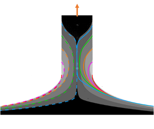
Figure 1. Sketches of the liquid ligament under consideration, showing the notations, in particular the locations $z_d$, $z_s$, and $L(t)$ where the boundary conditions are imposed. The origin of the cylindrical coordinate system is fixed at the initial position of the rod bottom. The initial configuration is presented in $(a)$, where a static meniscus is formed between the rod (located at $z=0$) and the bath (located at $z=-H_s$, dotted line) with a static meniscus angle $\theta _s = {\rm \pi}/2$, $g$ is gravity. The configuration in $(b)$ represents the liquid ligament at a later time, with a dynamic meniscus angle $\theta (t)$. The distance between the bath and the rod bottom is defined as the height $H(t)$, whereas the distance travelled by the rod is defined as the length $L(t)$.

1. (i) mass conservation equation

   (2.1)\begin{equation} \partial_t \,f^2 + \partial_z \left(\,f^2 u \right)= 0, \end{equation}

2. (ii) momentum equation

   (2.2)\begin{equation} f^2 \rho \left(\partial_t u + u \partial_z u \right) + f^2 \gamma \partial_z K + f^2 \rho g - 3 \mu \partial_z \left( f^2 \partial_z u \right)= 0, \end{equation}

3. (iii) mean curvature

   (2.3)\begin{equation} K(z,t) = \frac{1}{f \left[1 + (\partial_z f)^2 \right]^{1/2}} - \frac{\partial_{zz} f}{\left[1 + (\partial_z f)^2 \right]^{3/2}}, \end{equation}

where $u=u(z,t)$ is the extensional velocity and $K$ is the mean curvature. The first two terms in (2.2) account for inertia while the rest account, respectively, for capillary pressure, gravity and the extensional viscous stress (Trouton Reference Trouton1906). Note that we keep the full expression of the curvature in the one-dimensional model, as it allows us to have a full description of the ligament including the regions close to the bath and the rod. The same approaches have proven to provide good agreement with experimental results for ligaments (Eggers & Dupont Reference Eggers and Dupont1994; Clasen et al. Reference Clasen, Eggers, Fontelos, Li and Mckinley2006; van Hoeve et al. Reference van Hoeve, Gekle, Snoeijer, Versluis, Brenner and Lohse2010; Vincent, Duchemin & Le Dizès Reference Vincent, Duchemin and Le Dizès2014a; Martínez-Calvo et al. Reference Martínez-Calvo, Rubio-Rubio and Sevilla2018) and films (Champougny et al. Reference Champougny, Rio, Restagno and Scheid2017; Kofman et al. Reference Kofman, Rohlfs, Gallaire, Scheid and Ruyer-Quil2018). In particular, in Martínez-Calvo et al. (Reference Martínez-Calvo, Rubio-Rubio and Sevilla2018) the authors used it for the same geometry: a ligament and a liquid bath, with remarkable agreement.

2.2. Non-dimensionalised problem

Applying the following transformations,

(2.4a–d)\begin{gather} f \rightarrow R f , \quad z \rightarrow R z , \quad H \rightarrow R H , \quad L \rightarrow R L , \end{gather}

(2.4e–g)\begin{gather} K \rightarrow \frac{1}{R}K , \quad u \rightarrow \frac{\gamma}{\mu} u , \quad t \rightarrow \frac{\mu R}{\gamma} t , \end{gather}

the non-dimensional system of equations becomes

(2.5)\begin{gather} \partial_t\, f^2 + \partial_z (\,f^2 u)= 0, \end{gather}

(2.6)\begin{gather} \frac{1}{Oh^2} f^2 \left(\partial_t u + u \partial_z u \right) + f^2 \left( \partial_z K + Bo \right) - 3 \partial_z \left( f^2 \partial_z u \right)= 0, \end{gather}

(2.7)\begin{gather} K(z,t) = \frac{1}{f \left[1 + (\partial_z f)^2 \right]^{1/2}} - \frac{\partial_{zz} f}{\left[ 1 + (\partial_z f)^2 \right]^{3/2}} , \end{gather}

where $Bo$ and $Oh$ are the Bond and Ohnesorge numbers, respectively, defined as

(2.8a,b)\begin{equation} Bo= \frac{\rho g R^2}{\gamma}\text{ and} \quad Oh = \frac{\mu}{\sqrt {\rho \gamma R}}. \end{equation}

2.3. Initial and boundary conditions

The dynamic system requires two initial conditions respectively for $f$ and $u$. Naturally, we consider the static meniscus shown in figure 1 as the initial profile, with a static meniscus angle $\theta _s$ at the rod bottom, which is located at a dimensionless height $H_s$ above the bath. Simplified from (2.6) and (2.7), the non-dimensional static system is

(2.9)\begin{gather} K_{s}^\prime ={-} Bo , \end{gather}

(2.10)\begin{gather} K_{s} = \frac{1}{f_{s} \left(1 + \,f_{s}^{\prime 2} \right)^{1/2}} - \frac{f_{s}^{\prime \prime}}{\left(1 + \,f_{s}^{\prime 2} \right)^{3/2}} , \end{gather}

where $\,f_{s}(z)$ represents the static profile, $K_{s}(z)$ the static curvature and the prime denotes the derivative with respect to the $z$-coordinate. It is an ordinary differential equation system requiring three boundary conditions,

(2.11a)$$\begin{gather} K_{s} ( - H_{s} ) = 0, \end{gather}$$

(2.11b)$$\begin{gather}f_{s}^{\prime} ( - H_{s} ) ={-} \infty , \end{gather}$$

(2.11c)$$\begin{gather}f_{s}(0) = 1 , \end{gather}$$

where $-H_{s}$ is the position of the flat bath. However, an analytical solution does not obviously exist and a numerical method should be applied. Firstly, integrating (2.9) with respect to $z$ and using the boundary condition (2.11a) yields

(2.12)\begin{equation} K_{s} ={-} Bo \left( z + H_{s} \right) . \end{equation}

Substituting (2.10) into (2.12), we obtain

(2.13)\begin{equation} f_{s}^{\prime \prime} = Bo \left( z + H_{s} \right) \left( 1+ \,f_{s}^{\prime 2} \right)^{3/2} + \frac{1}{f_{s}} \left( 1 + \,f_{s}^{\prime 2} \right) . \end{equation}

To avoid the infinite boundary condition (2.11b), a position $z_s$ (see figure 1) close to the bath is used as the new boundary, i.e. $f_{s}^\prime (-H_{s})$ is replaced by $\,f_{s}^\prime ( z_s)$. According to Benilov & Oron (Reference Benilov and Oron2010), the asymptotic solutions of $f_s$ and $f_s^\prime$ close to the bath are

(2.14a)$$\begin{gather} f_{s} (z_s) = \frac{1}{\sqrt{Bo} } \left[ -\ln(a(z_s+H_{s})) - \frac{ \ln (-\ln(a(z_s+H_{s}))) }{2} - \frac{ 2 \ln (-\ln(a(z_s+H_{s})))-1 }{8 \ln(a(z_s+H_{s})) } \right] \nonumber\\ +\,O\left[ \frac{1}{\sqrt{Bo} } \left( \frac{ \ln(-\ln(a(z_s+H_{s}))) }{ \ln(a(z_s+H_{s})) } \right)^2 \right], \end{gather}$$

(2.14b)$$\begin{gather}f_{s}^\prime (z_s) ={-}\frac{1}{\sqrt{Bo} (z_s + H_{s})} \left[ 1+ \frac{1}{2 \ln ( a(z_s+H_{s}))} + \frac{3-2\ln(-\ln(a(z_s+H_{s})))}{8 \left( \ln(a(z_s+H_{s})) \right)^2} \right] \nonumber\\ +\,O\left[ \frac{2\ln(-\ln(a(z_s+H_{s}))) \left( 1- \ln(-\ln(a(z_s+H_{s})))\right)}{\sqrt{Bo} (z_s+H_{s}) \left( \ln a(z_s+H_{s})\right)^3} \right], \end{gather}$$

for $z_s \rightarrow -H_{s}$, where $a$ is a positive constant parameter. To obtain the static solution for a certain $Bo$ and a certain $H_s$, we seek for the corresponding parameter $a(Bo, H_s)$, namely shooting $f_s$ using (2.14) and adjusting the parameter $a$ until $f_s$ satisfies (2.11c). After obtaining the solutions, we calculate the static meniscus angles $\theta _s$ using $f_s^{\prime } (0)$ and find that two solutions with two $\theta _s$ (equivalently $a$) exist for most of the cases. Instead, we found it more convenient to parametrize the profile, the meniscus height and the parameter $a$ with $Bo$ and $\theta _s$ henceforth, namely $f_{s} (z, Bo, \theta _s)$, $H_{s} (Bo, \theta _s)$ and $a (Bo, \theta _s)$. For the following, we define the static meniscus height with a right angle meniscus as $H_{{\rm \pi} /2,s} (Bo) = H_s (Bo, {\rm \pi}/2)$, the maximum static meniscus height of a certain $Bo$ as $H_{b,s} (Bo)$, and the corresponding static meniscus angle as $\theta _{b,s}$, hence $H_{b,s} (Bo)=H_s (Bo,\theta _{b,s})$ and $\partial _{\theta _s} H_s (Bo, \theta _{b,s})=0$.

As presented in figure 1, one can draw ligaments from static menisci with various initial $\theta _s$. We show in Appendix A that the contraction stages are reasonably independent of the initial $\theta _s$, while the preliminary stages can be significantly influenced by $\theta _s$. We also show in § 6.2 that strong two-dimensional effects exist for ligaments close to the bath. Hence, to focus on the contraction dynamics and avoid the two-dimensional effects, we consider ligaments drawn from static menisci with $\theta _s={\rm \pi} /2$, i.e. from an initial height $H_{{\rm \pi} /2,s}$, in the present paper. The dimensionless initial conditions and the initial guess for $K$ are

(2.15a)$$\begin{gather} f(z,0) = \,f_{s} (z, Bo, {\rm \pi}/2), \end{gather}$$

(2.15b)$$\begin{gather}u(z,0) = \frac{Ca}{ f_{s}^2 (z,Bo,{\rm \pi}/2)} , \end{gather}$$

(2.15c)$$\begin{gather}K(z,0) = K_{s} (z, Bo, {\rm \pi}/2) , \end{gather}$$

where the capillary number $Ca$ is defined as

(2.16)\begin{equation} Ca = \frac{\mu U}{\gamma} . \end{equation}

According to the dimensionless transformations (2.4), $Ca$ henceforth is also mentioned as the dimensionless drawing velocity. We approximate the initial condition (2.15b) on $u$ by solving the stationary version of the conservation equation (2.5), using the constant speed at the rod as the boundary condition (see (2.17b)).

For the boundary conditions, using the same strategy as Champougny et al. (Reference Champougny, Rio, Restagno and Scheid2017), four boundary conditions are required, two at the rod side,

(2.17a)$$\begin{gather} f ( L(t) , t ) = 1 , \end{gather}$$

(2.17b)$$\begin{gather}u ( L(t) , t ) = Ca , \end{gather}$$

where $L(t)=Ca\, t$ is the dimensionless position of the rod, and two at a position $z_d$ close to the bath,

(2.18a)$$\begin{gather} \partial_z f(z_d,t) = \partial_z \,f_{s} (z_d, Bo, {\rm \pi}/2), \end{gather}$$

(2.18b)$$\begin{gather}K (z_d,t) = K_{s} (z_d, Bo, {\rm \pi}/2) . \end{gather}$$

The boundary conditions (2.18) impose that the profile sufficiently close to the bath ($-H_s < z < z_d$) generally remains static and can translate horizontally, as we only fix the slope and the curvature at that boundary. This quasi-static approach will later be validated in § 6.2, and can also be found in simulations of fibres (Ryck & Quéré Reference Ryck and Quéré1996), plates (Scheid et al. Reference Scheid, Delacotte, Dollet, Rio, Restagno, van Nierop, Cantat, Langevin and Stone2010) and films (Champougny et al. Reference Champougny, Rio, Restagno and Scheid2017) pulled out of a liquid bath. Note that, now there are two near-bath boundary positions $z_s$ and $z_d$ respectively for the static and the dynamic systems, with the relationship $-H_s < z_s < z_d <0$ (see figure 1). The reasons we do not keep $z_s$ in the dynamic system are: on the one hand, $-\partial _z \,f_{s} \approx 1/( Bo^{1/2} (z_s+H_s) )$ inferred from (2.14b) can be quite large for small $Bo$ and brings convergence difficulties for the partial differential equation (PDE) system; on the other hand, we show in Appendix B that the results are independent of the boundary position for $-\partial _z \,f_{s} \gtrsim 100$. In practice, we first solve the static system with $z_s = -0.999 H_{s}$ (ensuring the three decimal accuracy for $H_{s}$), obtaining $f_s$, $\partial _z f_s$ and $K_s$, then solve the dynamic system with $\partial _z f_s$ and $K_s$ at the position $z_d$ where $\partial _z \,f_{s} = -100$.

Based on the above, it results that the problem is governed by three independent parameters, the Bond number $Bo$, the capillary number $Ca$ and the Ohnesorge number $Oh$. Finally, the Ohnesorge number can also be expressed as a function of $Bo$,

(2.19)\begin{equation} Oh= \frac{\mu}{Bo^{1/4} \sqrt{\rho \gamma \ell_c }} , \end{equation}

such that only $Bo$ and $Ca$ should be varied independently for a given liquid. The dimensional physicochemical parameters we implement in the simulations (except Appendix C) are those of the $V5000$ silicone oil that we used in the experiments presented in § 5, namely $\mu = 4.92\ \text {Pa}\,\text {s}$, $\rho = 970\ \text {kg}\,\text {m}^{-3}$, $\gamma = 21.1\ \text {mN}\,\text {m}^{-1}$. We will show both numerically in Appendix C and experimentally in § 5 that drawing processes are reasonably independent of the Ohnesorge number for large-viscosity liquids with $\mu \geq 0.5\ \text {Pa}\,\text {s}$. The following parameter space is therefore considered in the present paper:

(2.20a)$$\begin{gather} 10^{{-}4} \leq Bo \leq 1 , \end{gather}$$

(2.20b)$$\begin{gather}10^{{-}5} \leq Ca \leq 1 , \end{gather}$$

(2.20c)$$\begin{gather}2.86 \leq Oh . \end{gather}$$

The static system of ordinary differential equations (2.13), (2.14) and (2.11c) is solved using MATLAB R2019b. The dynamic system of partial differential equations (2.5)–(2.7), supplemented by the initial conditions (2.15) and boundary conditions (2.17)–(2.18), is solved using the direct solver MUMPS in COMSOL 5.4. The computational domain $(z_d \le z \le L(t))$ is deforming with time due to the moving rod boundary, thus, the arbitrary Lagrangian–Eulerian (ALE) algorithm is applied for the moving mesh computation.

3.1. Basic results

We first consider the static meniscus height $H_s (Bo, \theta _s)$, the results of which are shown in figure 2$(a)$. For a certain $Bo$, $H_s$ first increases with $\theta _s$ and reaches the maximum value $H_{b,s}$ when $\theta _s=\theta _{b,s}$, then decreases with $\theta _s$. Note that, as given in (2.4), we non-dimensionalise the meniscus height with the rod radius $R$, the square of which appears in $Bo$. To show the dependence of meniscus heights on $R$ or equivalently on $Bo$, we present $\sqrt {Bo}\, H_{s}$ in figure 2$(b)$, namely the meniscus height non-dimensionalised by the capillary length $\ell _c$ ($\ell _c=\sqrt {\gamma /\rho g}$). It can be observed that though $H_{s}$ decreases with $Bo$, $\sqrt {Bo}\, H_{s}$ increases with $Bo$. The maximum height curve, as shown by the dashed line in figure 2, shows $\theta _{b,s}$ varying between 0 for $Bo \rightarrow \infty$ and ${\rm \pi} /2$ for $Bo \rightarrow 0$ (Padday & Pitt Reference Padday and Pitt1973). This critical curve further separates the static menisci into the unstable ($\theta _s < \theta _{b,s}$), the stable ($\theta _s > \theta _{b,s}$) and the neutral ($\theta _s = \theta _{b,s}$) regions (Padday & Pitt Reference Padday and Pitt1973; Pitts Reference Pitts1976; Benilov & Oron Reference Benilov and Oron2010). The static meniscus with $\theta _s = {\rm \pi}/2$ is therefore always stable, i.e. for all values of $Bo$. It thus appears as the suitable choice for the initial solution of the dynamic system of equations, as set up in § 2.3. Figure 3$(a)$ shows $H_s$ varying with $Bo$ for various $\theta _s$, $H_{s}$ tends to be linear to $\ln Bo$ with different slopes depending on $\theta _s$. The first derivative of $H_s$ with respect to $\ln Bo$ is presented in figure 3$(b)$, showing that the linear relationship holds when $Bo \lesssim 10^{-2}$, and the slopes tend to be the same for supplementary angles. This relationship is mentioned as the Derjaguin–James formula in the literature Tang (Reference Tang and Cheng2019), which has been analysed analytically James (Reference James1974), but only at the leading order. A similar behaviour was reported by Kovitz (Reference Kovitz1975), the author having observed that the envelope of menisci of various radii behaves like $y \sim - x \ln x$ with $y = \sqrt {Bo} (z+H_{s})\, {\rm and}\ x = \sqrt {Bo} \,f_{s}$, when $Bo \rightarrow 0$.

Figure 2. Dimensionless height of the static meniscus $H_{s}$ in $(a)$, and rescaled height $\sqrt {Bo}\, H_{s}$ in $(b)$, varying with static meniscus angle $\theta _s$ for different values of $Bo$. The dashed lines represent the maximum height cases for $\theta _s = \theta _{b,s}$.

Figure 3. Dimensionless height of the static meniscus $H_{s}$ in $(a)$ and first derivative of $H_s$ with respect to $\ln Bo$ in $(b)$, varying with $Bo$ for different values of the static meniscus angle $\theta _s$. The dashed lines represent the maximum height cases $H_{b,s}$ for $\theta _s = \theta _{b,s}$, the squares in $(b)$ represent the analytical values of $(\sin \theta _s )/2$ (see (3.11a)).

3.2. Static meniscus in the low gravity case

As suggested by the results in the previous section, some simplifications can arise in the low gravity case corresponding to $Bo \lesssim 10^{-2}$. To unravel the underlying mechanism, we introduce the radial curvature $K_r$, the axial curvature $K_a$ and define $K_g$ as the gravity term,

(3.1a–c)\begin{equation} K_r = \frac{1}{f_{s} \left(1 + \,f_{s}^{\prime 2} \right)^{1/2}}, \quad K_a ={-} \frac{f_{s}^{\prime \prime}}{\left(1 + f_{s}^{\prime 2} \right)^{3/2}} , \quad K_g ={-} Bo ( z + H_{s}) . \end{equation}

Then the static system (2.12) can be written as a balance between the three components of pressure, $K_r + K_a = K_g$. Typical profiles and comparisons of the three terms for $\theta _s={\rm \pi} /2$ are presented in figure 4. At the rod boundary ($z=0$), we have boundary conditions $f_{s} = 1$ and $f_{s}^\prime = \cot \theta _s$, leading to a finite radial curvature $K_r$. On the other hand, the gravity term $K_g$ is at least one order of magnitude smaller than $K_r$ for $Bo \lesssim 10^{-2}$. In fact, not only at the rod boundary but also from a position slightly above the bath, the relationship $K_r \approx - K_a \gg K_g$ holds, as shown in figure 4$(b)$. The top region of the static meniscus therefore can be described as

(3.2)\begin{equation} \frac{1}{f_{s} \left(1 + \,f_{s}^{\prime 2} \right)^{1/2}} - \frac{f_{s}^{\prime \prime}}{\left(1 + \,f_{s}^{\prime 2} \right)^{3/2}} \approx 0 \quad \text{for } Bo \lesssim 10^{{-}2} \text{ and }z \gnsim -H_{s}, \end{equation}

in which $O(Bo)$ terms have been omitted. Note that we use the symbol $\gnsim -H_{s}$ to represent the position away from the bath, we will later use the opposite symbol $\lnsim 0$ to represent the position away from the rod, namely the top region and the bottom region, respectively. The solution of the top region static meniscus with $\theta _s={\rm \pi} /2$ can be found in de Gennes, Brochard-Wyart & Quéré (Reference de Gennes, Brochard-Wyart and Quéré2004), which turns out to be a catenoid. In Appendix D we derive the solutions for arbitrary $\theta _s$, obtaining

(3.3)$$\begin{gather} f_{s, top} (z, \theta_s) \approx \cos^2 \left( {\frac {\theta_s}{2} } \right) \exp \left(\frac{z}{\sin \theta_s}\right) + \sin^2 \left({\frac {\theta_s}{2} }\right) \exp \left(\frac{- z}{\sin \theta_s}\right) \nonumber\\ \text{for } Bo \lesssim 10^{{-}2} \text{ and }z \gnsim -H_{s} . \end{gather}$$

This profile being independent of $Bo$, it automatically describes the entire meniscus profile in the agravic limit, i.e. for $Bo \rightarrow 0$.

Figure 4. Typical results of static menisci for $\theta _s = {\rm \pi}/2$ and different values of $Bo$. $(a)$ Static profiles in solid lines as compared with the static meniscus in the agravic limit (see (3.3)) as a dashed line. $(b)$ The radial curvatures $K_r$ in solid lines, the axial curvature $-K_a$ in dashed lines and the gravity term $K_g$ in dotted lines.

In the meniscus region away from the rod the derivative $f_{s}^\prime$ becomes large, i.e. $\,f_{s}^{\prime 2} \gg 1$. Following the work of Benilov & Oron (Reference Benilov and Oron2010), the bottom region of the static meniscus can then be described as

(3.4)\begin{equation} - \frac{1}{f_{s} \,f_{s}^\prime} + \frac{f_{s}^{\prime \prime}}{f_{s}^{\prime 3}} \approx{-} Bo ( z + H_{s})\quad \text{for } z \lnsim 0 . \end{equation}

The solution of the bottom region has the form

(3.5)\begin{equation} f_{s} (z, Bo, \theta_s) \approx \frac{1}{\sqrt Bo} F (x) \quad \text{for } x >0 , \end{equation}

where $x = a (z+H_{s})$, in which $a=a (Bo, \theta _s)$ is the positive parameter in (2.14b), and $F(x)$ is a certain function to be determined. As shown in figure 5$(a)$, $a(Bo, \theta _s)$ tends to be symmetric around ${\rm \pi} /2$ and converges to a certain $a(\theta _s)$ for $Bo \lesssim 10^{-2}$, where the explicit expression for $a(\theta _s)$ is derived below. Meanwhile the numerical result of $F(x)$ in figure 5$(b)$ shows that $\ln F(x)$ is linear to $x$ for $x \gnsim 0$, namely

(3.6)\begin{equation} F (x) = \exp(m x +n) \quad \text{for } x \gnsim 0 , \end{equation}

where $m = -1.251$ and $n = 0.108$ are fitted from the numerical results. We then obtain the bottom region static meniscus,

(3.7)\begin{equation} f_{s, bot} (z, Bo, \theta_s) \approx \frac{1}{\sqrt Bo} F ( a (\theta_s) ( z+H_{s}) ) \quad \text{for } Bo \lesssim 10^{{-}2} \text{ and }z \lnsim 0 . \end{equation}

Figure 5. $(a)$ Parameter $a$ varying with $\theta _s$ for different values of $Bo$, and the analytical solution $a(\theta _s)$ (see (3.11b)) is the solid line. $(b)$ The numerical result of $F (x)$ is the solid line, and the asymptote (see (3.6)) is the dashed line.

In addition to the top and bottom regions, there is the middle region that should satisfy both conditions, namely, $K_r \approx -K_a \gg K_g$ and $\,f_{s}^{\prime 2} \gg 1$. The middle region of the static meniscus therefore can be described as

(3.8)\begin{equation} - \frac{1}{f_{s} \,f_{s}^\prime} + \frac{f_{s}^{\prime \prime}} {f_{s}^{\prime 3}} \approx 0 \quad \text{for } Bo \lesssim 10^{{-}2} \text{ and } -H_{s} \lnsim z \lnsim 0 . \end{equation}

The analytical solution can be obtained as

(3.9)\begin{equation} f_{s, mid} (z, Bo, \theta_s) \approx \exp( k z + b ) \quad \text{for } Bo \lesssim 10^{{-}2} \text{ and }-H_{s} \lnsim z \lnsim 0 , \end{equation}

where $k$ and $b$ are parameters depending on $Bo$ and $\theta _s$. Equations (3.3), (3.7) and (3.9) represent the three regions of the static meniscus in the low gravity case, and as shown in figure 4$(a)$, the middle region becomes longer with smaller $Bo$. To match the different regions, we compare the logarithms of (3.3), (3.7), (3.9), and use (3.6), yielding

(3.10a)$$\begin{gather} k \approx{-} \frac{1}{\sin \theta_s} \approx m a , \end{gather}$$

(3.10b)$$\begin{gather}b \approx 2 \ln \sin {\frac{\theta_s}{2}} \approx m a H_{s} + n - \frac{1}{2}\ln Bo , \end{gather}$$

for $Bo \lesssim 10^{-2}$, where only the second term of (3.3) is used here since the first term is negligible for $z \lnsim 0$. Combining (3.10) gives the relationships

(3.11a)$$\begin{gather} H_{s} (Bo, \theta_s) \approx{-} \frac{1}{2} \sin \theta_s \ln Bo + \sin \theta_s \left( n- 2 \ln \sin {\frac{\theta_s}{2}} \right) , \end{gather}$$

(3.11b)$$\begin{gather}a(Bo, \theta_s) \approx a(\theta_s) ={-}\frac{1}{m \sin \theta_s} , \end{gather}$$

for $Bo \lesssim 10^{-2}$. Equation (3.11a) is actually the Derjaguin–James formula, which reveals the linear relationship between $H_{s}$ and $\ln Bo$ we observed in figure 2$(b)$ for $Bo \lesssim 10^{-2}$, while (3.11b) gives the explicit expression of the parameter $a$ in this low gravity case reproduced in figure 5$(a)$. Finally, we derive from (3.11a) the explicit expression for $H_{{\rm \pi} /2,s}$,

(3.12)\begin{equation} H_{{\rm \pi}/2,s} (Bo) \approx{-}\dfrac{1}{2}\ln Bo+ \ln 2 + n \quad \text{for } Bo \lesssim 10^{{-}2}. \end{equation}

4.1. Basic results

Typical profiles $f(z,t)$ and axial velocities $u(z,t)$ are presented in figure 6, at different lengths $L(t)$ during drawing. At $L=0$, a static meniscus forms between the liquid bath and the rod, the bottom of which is initially located at $z=0$, and set into motion at a constant dimensionless velocity $Ca$. As the rod goes up, the ligament extends axially and contracts radially, whereas the bottom profile remains static. In a first stage for $L \lesssim 2.3$, the ligament evolves with the following behaviour: the middle part of the profile is generally tangent to the dashed line in figure 6$(b)$, and the velocity stays in the range $0 \lesssim u \lesssim Ca$ as seen in figure 6$(c)$. The dashed line corresponds to (3.9) with $\theta _s = {\rm \pi}/2$, namely $f_{s, mid}=\exp (-z-\ln 2)$. The instability effect is not clearly observable in the first behaviour, which is thus referred to as the ductility stage. As the rod is drawn higher for $L > 2.3$, it enters the capillarity stage, in which the former ductility behaviour fails due to the observable capillary instability. As shown in figure 6$(b)$, the middle part of the profile departs from the dashed line and develops into a local symmetric shape around the thinnest position, while the axial velocity forms a bimodal shape with a peak value $u > Ca$ and a trough value $u < 0$. The ligament length at which the ductility/capillarity transition occurs is defined as the transition length $L_t$. We here use the result $L_t \approx 2.3$ of the agravic limit obtained in § 4.2 to approximately identify the transition, marked by the squares in figure 6. Finally, when the thinnest radius $\,f_{ min} \ll 1$, the process enters the pinch-off stage. As we are concerned with large-viscosity ligaments for $Oh \geq 2.86$, the process first enters the viscous regime (Papageorgiou Reference Papageorgiou1995; Eggers Reference Eggers2005) with the well-defined dimensionless relationship $\,f_{ min} = 0.0709 (t_b-t)$. The first derivative of $\,f_{ min}$ with respect to $t$ is shown in figure 7, for a typical Bond number $Bo=10^{-2}$ and different velocities in $(a)$, and a typical dimensionless velocity $Ca=0.1$ and different $Bo$ in $(b)$. The derivative converges to $-0.0709$ when $t_b-t \lesssim 0.1$. Hence, the drawing length $L_p$ within the pinch-off stage of duration $t_b-t$ verifies

(4.2)\begin{equation} L_{p} \lesssim 0.1 Ca \ll 0.1 L_b , \end{equation}

since $Ca \ll L_b$ as observed below in figure 8$(a)$. As the ligament continues contracting, it will later enter the final viscous-inertial regime (Eggers Reference Eggers1993, Reference Eggers2005). Now, we do not elaborate more on the pinch-off stage as the additional length (4.2) indicates it has a negligible contribution to the breakup length. The pinch-off stage is here used as the stop criterion for the simulation, i.e. when the minimum radius reaches $10^{-5}$, which ensures a numerical accuracy of three decimals for $L_b$.

Figure 6. Dimensionless profiles $f(z,t)$ in $(a)$ linear and $(b)$ log scales, axial velocities $u(z,t)$ in $(c)$ at different drawing lengths $L(t)=Ca \, t$ during the drawing for $Bo=10^{-2}$ and $Ca=0.3$. The bath is located at $-H_{ {\rm \pi}/2,s}=-3.111$, as shown as a dotted line in $(a)$. The ligament breakup, defined as the instant when the minimum dimensionless profile radius reaches $10^{-5}$, occurs at $L_b=3.065$ (presented in the inset of $b$). The inset in $(a)$ shows the dynamic meniscus angle $\theta$ varying with $L(t)$, with the minimum value $\theta _{ min}$ marked by a circle. The squares indicate the ligament length $L_t \approx 2.3$ when the ductility/capillarity transition occurs. The dashed line in $(b)$ represents the line of the middle region static meniscus in the agravic limit, the dash–dotted line in $(c)$ represents $u=Ca$.

Figure 7. First derivative of $\,f_{ min}$ with respect to $t$, converges to $-0.0709$ when it enters the viscous pinch-off regime. $(a)\ $ Bound number $Bo=10^{-2}$ with different Ca, $(b)$ the dimensionless drawing velocity $Ca=0.1$ with different $Bo$.

Figure 8. $(a)$ Breakup lengths $L_b (Bo,Ca)$ vs $Ca$ for different values of $Bo$ in solid lines, the static limit $L_{b,s} (Bo)$ in dotted lines, the agravic limit $L_{b,a} (Ca)$ as a dashed line. The inset shows $L_b$ vs $Bo$ for $Ca=1$. $(b)$ Breakup heights $H_b (Bo,Ca)$ vs $Ca$ for different values of $Bo$ in solid lines, the maximum static meniscus height $H_{b,s} (Bo)$ in dash–dotted lines.

We also present the development of the dynamic meniscus angle $\theta$ in the inset of figure 6$(a)$, showing that $\theta$ first decreases then increases with $L$, and the minimum dynamic meniscus angle $\theta _{ min}=41.4^\circ$ occurs at $L= 1.20$. This result validates the hypothesis that the liquid ligament remains pinned at the edge of the rod bottom, provided the receding contact angle of the liquid on the rod bottom is smaller that $\theta _{ min}$, which is the case in the experiments presented in § 5.

Breakup lengths $L_b$ varying with $Ca$ for typical values of $Bo$ are presented in figure 8$(a)$, compared with the static limit $L_{b,s}$ and the agravic limit $L_{b,a}$, the corresponding regimes are shown in figure 9. The static breakup length is defined as $L_{b,s}(Bo) = H_{b,s}(Bo) - H_{{\rm \pi} /2,s} (Bo)$. The agravic limit $L_{b,a}(Ca)$ is obtained numerically by omitting the gravity term in the dimensionless momentum equation (2.6) and starting with the agravic static meniscus (3.3). As one can expect intuitively, the breakup length increases with the drawing velocity. For very slow drawing, i.e. $Ca \rightarrow 0$, $L_b$ tends to $L_{b,s}$ such as the drawing of ligaments can be regarded as a quasi-static process. As shown in figure 8$(a)$, $L_b$ converges to $L_{b,a}$ for $Bo \lesssim 10^{-2}$ (see the inset) and $Ca \gtrsim Bo$, indicating that gravity has a negligible influence on the drawing dynamics, since $Bo \lesssim 10^{-2}$ ensures that the initial meniscus approximates the agravic static meniscus, while $Ca \gtrsim Bo$ ensures the extensional viscous forces to dominate the gravitational drainage (Champougny et al. Reference Champougny, Rio, Restagno and Scheid2017). These cases with low gravity and not slow drawing velocities are defined as the agravic drawing (see figure 9), whose results are thus identical to the agravic limit $L_{b,a}$,

(4.3)\begin{equation} L_b (Bo, Ca) \approx L_{b,a} (Ca) \quad \text{for } Bo \lesssim 10^{{-}2} \text{ and } Ca \gtrsim Bo . \end{equation}

Note that, for convenience, $L_{b,a}$ can be fitted by $4.661Ca^{0.609}+1.072Ca^{0.157}$ (without physical background). Breakup heights $H_b$ are shown in figure 8$(b)$, which generally increases with the same law for the dimensionless drawing velocity $Ca$, and generally decreases linearly with $\ln Bo$. For the agravic drawing regime, substituting (3.12) and (4.3) into (4.1) yields

(4.4)\begin{equation} H_{b} (Bo, Ca) \approx H_{{\rm \pi}/2,s}(Bo) + L_{b,a}(Ca) \quad \text{for } Bo \lesssim 10^{{-}2} \text{ and } Ca \gtrsim Bo. \end{equation}

Figure 9. Regimes of ligaments drawn out of a pure-liquid bath in our parameter space, the static limit for $Ca \rightarrow 0$, the agravic limit for $Bo \rightarrow 0$, the low gravity case for $Bo \lesssim 10^{-2}$ and the agravic drawing for $Bo \lesssim 10^{-2}$ and $Ca \gtrsim Bo$.

4.2. Transient drawing dynamics

It is a fact that the breakup length (height) does result from the interaction of ductility and capillarity (Ide & White Reference Ide and White1976). However, the transient dynamics of ligaments drawing have rarely been studied. As presented in figure 8 and (4.3), the agravic drawing cases represent the main feature of the drawing dynamics, it is therefore reasonable to focus on the agravic limit $L_{b,a}$ (with no gravity) to unravel its mechanism. To describe the development of the ligament quantitatively, we define the contraction and the contraction velocity as

(4.5a)$$\begin{gather} \eta (Ca, L(t)) = 1 - \,f_{ min} (Ca, L(t)) , \end{gather}$$

(4.5b)$$\begin{gather}\xi (Ca, L(t)) = \frac{\partial \eta}{\partial t} = Ca \frac{\partial \eta}{\partial L} . \end{gather}$$

Contractions $\eta$ for different $Ca$ are presented in figure 10$(a)$, starting at 0 and breaking at 1. Note that the squares in figure 10 are the transition lengths $L_t (Ca)$ which are later obtained by (4.10). For $Ca \lesssim 10^{-2}$, $\eta$ first increases slowly with $L$ in the ductility stage ($L \lesssim L_t$) and then suddenly increases more rapidly ($L > L_t$) in the capillarity stage. This transition corresponds to the failure of the ductility behaviour (see figure 6$b{,}c$), whereas it is less clear for $Ca > 10^{-2}$. The corresponding contraction velocities $\xi$ are shown in figure 10$(b)$, with $\xi = 0.0709$ when it enters the pinch-off stage, as shown in the inset of figure 10$(b)$ and discussed in § 4.1. Transitions in the slope of $\xi$ can also be clearly observed when $Ca \lesssim 10^{-2}$.

Figure 10. Results of the agravic limit ($Bo = 0$) with different dimensionless drawing velocity $Ca$. Dimensionless contractions in $(a)$, numerical results $\eta$ in solid lines and the ductility solution $\eta _{d}$ is a dashed line. Dimensionless contraction velocities in $(b)$, numerical results $\xi$ in solid lines (final values in the inset), the ductility-induced $\xi _d$ in dashed lines and the capillarity-induced $\xi _c$ is a dash–dotted line. The squares represent the transition lengths $L_t$ (obtained by solving $\xi _d=\xi _c$, i.e. the lengths corresponding to the intersections of the dashed lines and the dash–dotted line), separating the whole process into a ductility stage ($0 < L \lesssim L_t$) and a capillarity stage ($L_t < L < L_b$).

4.2.1. Determining the transition length

Obviously, determining the transition length $L_t$ is the principal step of unravelling the transient drawing dynamics. We assume the capillary instability to be determined by the transient profile, which corresponds to the ductility profile in the ductility stage (see figure 6$b$). Notice the ductility behaviour could be observed in all cases, indicating that they could be approximately described in an identical spatial function $f_d(z,L)$ for all $Ca$, which can help us to obtain the ductility-induced and capillarity-induced contraction velocities independently. We therefore first seek the approximate ductility solution and then determine the ductility/capillarity transition by comparing the respective contraction velocities.

For the agravic limit, the initial profile can be derived by substituting $\theta _s={\rm \pi} /2$ into the agravic static meniscus (3.3), yielding

(4.6)\begin{equation} f (z,0) = \tfrac{1}{2} \left( e^z +e^{{-}z} \right) , \end{equation}

which is a catenoid. As presented in figure 6$(b)$, the bottom profile remains quasi-static during the whole process. We thus assume the approximate ductility solution in the form

(4.7)\begin{equation} f_{d} (z,t) = \tfrac{1}{2} \left( E(t) e^z +e^{{-}z} \right) , \end{equation}

where $E(t)$ is a new function depending on $t$. Substituting (4.7) into the boundary condition (2.17a) at the rod bottom, we obtain the approximate ductility solution, written in the spatial form

(4.8)\begin{equation} f_{d} (z,L) = \frac{1}{2} \left( \frac{ 2 e^L -1}{e^{2L}} e^z +e^{{-}z} \right) . \end{equation}

Notice $f_d(z,L)$ is referred hereafter to as the ductility solution. The corresponding contraction and contraction velocity could be derived by minimizing (4.8) and substituting the result into (4.5), which gives

(4.9a)$$\begin{gather} \eta_{d} (L) = 1 - \frac{\sqrt {2 e^L -1}}{e^L} , \end{gather}$$

(4.9b)$$\begin{gather}\xi_{d} (L, Ca) = Ca \left( \frac{\sqrt{2 e^L -1}}{e^L} - \frac{1}{\sqrt{2 e^L -1}} \right) . \end{gather}$$

As shown in figure 10$(a)$, $\eta _{d}$ is a spatial function identical for all $Ca$, while figure 10$(b)$ shows that $\xi _{d}$ is a family of curves proportional to $Ca$. They fit well the numerical results in the ductility stage for $Ca \lesssim 10^{-3}$, and approach the tendency for $Ca >10^{-3}$.

After the ligament is drawn for a while in the ductility stage, the profile can be approximately described by $f_d(z,L)$, which is then used to infer the capillarity-induced contraction. We consider the process starting from $\,f_{d}(z,L)$ with zero drawing speed, and use the numerical method described in § 2 to solve the nonlinear transient problem with modified initial and boundary conditions, obtaining the capillarity-induced contraction velocity $\xi _c (L)$, as detailed in Appendix E. Results are presented in figure 10$(b)$ as a dash–dotted line, showing that $\xi _{c}$ increases rapidly with $L$.

With contraction velocities $\xi _{d}$ and $\xi _{c}$, the transition length $L_t(Ca)$ can be obtained by solving

(4.10)\begin{equation} \xi_{d} (Ca, L_t) = \xi_{c} (L_t) , \end{equation}

i.e. the intersections of the dashed lines and the dash–dotted line shown in figure 10$(b)$. In figure 10$(a{,}b)$, $L_t$ for typical values of $Ca$ are marked by squares on the one-dimensional solutions in solid lines. They fit the numerical ductility/capillarity transition regions quite well, indicating that the transition indeed results from the competition of contraction velocities induced by ductility and capillarity.

4.2.2. Capillary instability for the stretched ligaments

We show in the following that the transient drawing dynamics can be further explained by the transient development of the growth rate. Defining $\sigma (L)$ as the estimate of the transient growth rate for each ductility profile $f_d(z,L)$, yielding $\sigma (L) = \xi _c (L)/ \eta _d (L)$. We show $\sigma (L)$ in figure 11$(a)$, compared with the analytical solution $\sigma _{cy}$ of a viscous cylindrical ligament whose dimensionless radius is unity. We observe that $\sigma \rightarrow 0$ when $L \rightarrow 0$, which agrees with the neutrally stable property of the initial static meniscus. As $L$ increases, $\sigma$ increases while the profile becomes thinner and longer, and $\sigma$ gradually tends to the same magnitude as $\sigma _{cy}$ for $L \gtrsim 1$. To understand the underlying mechanism, we display the characteristic curvatures of $f_d (z,L)$ at the $\,f_{ min}$ position, namely $K_{c,r}$ for the radial curvature, $-K_{c,a}$ for the axial curvature and $K_c$ for the mean curvature, as shown in figure 11$(b)$. The radial curvature destabilizes the ligaments: for $L\lesssim 1$, $K_{c,r} \approx -K_{c,a}$, leading to very small $K_c$ and $\sigma$; for $L > 1$, $K_{c,r}$ dominates the mean curvature $K_c$, leading to $\sigma$ close to $\sigma _{cy}$. Related findings can be found in Rubio-Rubio et al. (Reference Rubio-Rubio, Sevilla and Gordillo2013), Gordillo, Sevilla & Campo-Cortés (Reference Gordillo, Sevilla and Campo-Cortés2014) and Martínez-Calvo et al. (Reference Martínez-Calvo, Rubio-Rubio and Sevilla2018), where the authors pointed out the essential stabilizing role played by the axial curvature. In particular, Martínez-Calvo et al. (Reference Martínez-Calvo, Rubio-Rubio and Sevilla2018) found that the growth rate tends to a very small value when the ligament profile tends to a neutral meniscus, while it tends to a finite value when the ligament is quite long, which is similar to our results in figure 11$(a)$.

Figure 11. $(a)\ $Estimate of the transient growth rate $\sigma (L)$ for different profiles $f_d(z,L)$, compared with the analytical maximum growth rate $\sigma _{cy}$ of a viscous cylindrical ligament (of unit dimensionless radius). $(b)$ Characteristic values of the radial curvature ($K_{c,r}$), of the axial curvature ($-K_{c,a}$), and of the mean curvature ($K_c$), for $f_d(z,L)$ at the $f_{ min}$ position.

5.1. Experimental set-up

Ligaments are drawn out of a pure-liquid bath by a steel cylindrical rod of radius $R = 75$, 250 or $750\ \mathrm {\mu }\textrm {m}$. As sketched in figure 12$(a)$, the rod is attached on a vertical translation plate, which can be lifted at a constant velocity $0.01\ \text {mm}\,\text {s}^{-1} \leq U \leq 10\ \text {mm}\,\text {s}^{-1}$ by a motorised screw stage. The acceleration distance is tested to be less than $3 \ \mathrm {\mu }\textrm {m}$ even for the highest velocity of $10\ \text {mm}\,\text {s}^{-1}$, which is negligible compared with the rod radius. A liquid container with diameter $120\ \text {mm}$ and depth $40 \ \text {mm}$ is put on a fixed platform. We use silicone oil to form the ligaments, which can be considered as a model Newtonian pure liquid. Table 1 shows the physicochemical parameters of the different silicone oils used in the experiments, the viscosities and surface tensions are respectively measured with a viscosimeter (NDJ-5S, LICHEN) and a tensiometer (MC-1021, MINCEE) at the temperature $25\,^{\circ }\textrm {C}$. The results of ligament drawing are recorded by a high-speed camera (Phantom V2512, USA) fitted with a Nikkro 100 mm microlens at frame rates ranging from 2000 to 5000 frames per second and resolution of $3 - 13 \ \mathrm {\mu }\textrm {m}$ per pixel, with flickerless backlighting produced by a high-intensity LED lamp.

Figure 12. $(a)$ Sketch of the experimental set-up. $(b - d)$ Sketches (top) and experimental pictures (bottom, for $R= 750\ \mathrm {\mu }\textrm {m}$, $Ca=0.108$) of the critical states with respectively the dimensional height $H^*=0$, $H_{{\rm \pi} /2,s}^*$ and $H_{b, exp}^*$. The dotted lines (top) and the bottom edges (bottom) represent the flat surface of the bath.

Table 1. Main physicochemical parameters of the silicone oils used in the experiments, all parameters are given at $25\,^{\circ }\textrm {C}$.

We use symbols with the superscript $()^*$ to represent the dimensional experimental variables. The rod is initially just attached to the flat surface of the bath, namely at the dimensional height $H^*=0$, as shown in figure 12$(b)$. The liquid climbs up along the outside of the rod and forms an outside static meniscus (James Reference James1974), which is different from the static meniscus we considered in the present paper, namely the meniscus attached to the edge of the rod bottom. The experiments are operated in the following three steps: (i) lift the rod up from $H^*=0$ slowly at a constant velocity $U = 0.01\ \text {mm}\,\text {s}^{-1}$, until it reaches a dimensional height $H_{{\rm \pi} /2,s}^*$ (see figure 12$(c)$, $H_{{\rm \pi} /2,s}^*$ is defined as $H_{{\rm \pi} / 2,s} R$, inferred from the static solution); (ii) stop the rod at the position for 20 s; (iii) lift the rod up at a prescribed constant velocity $0.01\ \text {mm}\,\text {s}^{-1} \leq U \leq 10\ \text {mm}\,\text {s}^{-1}$, the ligament breaks at a dimensional height $H_{b, exp}^*$ (see figure 12$d$). During step (i), the outside meniscus gradually retreats from the rod side and transforms into the static meniscus considered in this paper as the initial condition. By doing this, we obtain a perfectly wetting rod with a very small receding contact angle (ideally zero), meaning that the dewetting phenomenon will not occur in our experiments, which is also validated in the experimental results. In order to ensure that the meniscus we start with in step (iii) is the static one, we stop the rod in step (ii) for a duration much larger than the typical time scale $\mu R / \gamma$, which is at most $2.04\ \text {s}$ for the largest rod ($R= 750\ \mathrm {\mu }\textrm {m}$) and the most viscous oil ($V60000$). Step (iii) corresponds to the ligament drawing considered in the present paper. The dimensional breakup heights $H_{b, exp}^{*}$ are identified from the final breakup images, the corresponding dimensionless breakup heights $H_{b, exp}$ are obtained by $H_{b, exp}=H_{b, exp}^{*}/R$. The experimental errors are $\lesssim 0.5\,\%$ for the breakup height, $2\,\%$ for the viscosity and $0.05\,\%$ for the surface tension.

5.2. Experimental results

We first investigate the influence of the drawing velocity, using the silicone oils of various viscosities shown in table 1 and the same rod of radius $R= 750\ \mathrm {\mu }\textrm {m}$ ($Bo=2.5\times 10^{-1}$). The dimensionless results $H_{b, exp}$ are shown in figure 13$(a)$, compared with the one-dimensional prediction $H_b$. Data points are obtained with viscosities varying over two orders of magnitude and drawing velocities varying over three orders of magnitude. Each point is the average value over three measurements, with the standard deviation being smaller than the size of the symbols. As shown in figure 13$(a)$, $H_{b, exp}$ for all three oils collapse onto a single master curve when plotted vs $Ca$, indicating that inertia has little effect on the drawing dynamics (see also Appendix C). This was also the case for films (Champougny et al. Reference Champougny, Rio, Restagno and Scheid2017), but with a different destabilizing mechanism taking its origin in van der Waals forces while ligaments are destabilized by capillary forces. Data for $V60000$ lie slightly above those of $V500$ and $V5000$, which should be attributed to the coating effect during step (i) in experiments (see § 6.2). The experimental results $H_{b, exp}$ agree well with the one-dimensional predictions $H_b$, while small deviations could be observed: $H_{b, exp}$ are lower than $H_b$ for $Ca \lesssim 0.2$, while higher for $Ca > 0.2$.

Figure 13. $(a)$ The dimensionless breakup heights $H_{b, exp}$ in symbols for three different silicone oils, using the same rod of radius $R = 750\ \mathrm {\mu }\textrm {m}$ ($Bo=2.5\times 10^{-1}$), compared with the corresponding one-dimensional predictions $H_b$ shown as a solid line. $(b)$ The dimensionless breakup heights $H_{b, exp}$ in symbols for $V5000$ silicone oil, using rods of radii $R=75\ \mathrm {\mu }\textrm {m}$ ($Bo=2.5\times 10^{-3}$), $250\ \mathrm {\mu }\textrm {m}$ ($Bo=2.8\times 10^{-2}$) and $750 \ \mathrm {\mu }\textrm {m}$ ($Bo=2.5\times 10^{-1}$), compared with the corresponding one-dimensional predictions $H_b$ in solid lines.

The influences of the rod radius are then investigated, using the $V5000$ silicone oil, and rods of different radii $R= 75\ \mathrm {\mu }\textrm {m}$ ($Bo=2.5\times 10^{-3}$), $250\ \mathrm {\mu }\textrm {m}$ ($Bo=2.8\times 10^{-2}$) and $750 \ \mathrm {\mu }\textrm {m}$ ($Bo=2.5\times 10^{-1}$). Results are presented in figure 13$(b)$, each point is again repeated three times. For all three rods, $H_{b, exp}$ agree well with the corresponding $H_b$, showing small deviations similar to those observed in figure 13$(a)$. We will show in § 6 that, except for the slight elevation of the $V60000$ silicone oil, the deviations between $H_{b, exp}$ and $H_b$ are mainly due to two-dimensional effects but not the coating effect.

6.1. Two-dimensional model

The flow in the liquid ligament and inside the bath can be modelled with the dimensionless mass conservation and the dimensionless momentum equations

(6.1a)$$\begin{gather} \boldsymbol{\nabla} \boldsymbol{\cdot} \boldsymbol{v} = 0, \end{gather}$$

(6.1b)$$\begin{gather}\frac{1}{Oh^2} \left(\partial_t \boldsymbol{v} + \boldsymbol{v} \boldsymbol{\cdot} \boldsymbol{\nabla} \boldsymbol{v} \right)= \boldsymbol{\nabla} \boldsymbol{\cdot} \textsf{$\mathbf{\tau}$} - Bo \boldsymbol{e}_z, \quad \text{at}\ \mathcal{V} , \end{gather}$$

where $\textsf{$\mathbf{\tau}$} =-p \boldsymbol{\mathsf{I}} + \boldsymbol {\nabla } \boldsymbol {v} + (\boldsymbol {\nabla } \boldsymbol {v})^T$ is the stress tensor, $\boldsymbol {v}$ is the velocity and $p$ is the pressure. These equations hold at any position, $\boldsymbol {x}$, of the deformable axisymmetric domain $\mathcal {V}(t)$ occupied by the liquid. To deal with the deformable domain, the ALE method is used, as in Martínez-Calvo et al. (Reference Martínez-Calvo, Rivero-Rodríguez, Scheid and Sevilla2020), and Rivero-Rodriguez, Perez-Saborid & Scheid (Reference Rivero-Rodriguez, Perez-Saborid and Scheid2021). In this method, any point $\boldsymbol {X}$ of a reference domain $\mathcal {V}_{ ref}$ is transformed into a point in the actual domain, such that $\boldsymbol {x}=\boldsymbol {x}(\boldsymbol {X},t) \in \mathcal {V}$. We choose the mapping $\boldsymbol {q} = \boldsymbol {x}-\boldsymbol {X}$ to fulfil

(6.2)\begin{equation} \nabla^2 \boldsymbol{q} = 0 \quad\text{at}\ \mathcal{V}, \end{equation}

for which boundary conditions must be imposed. The boundary of $\mathcal {V}$ consists of the truncation boundary of the infinite bath, $\varSigma _{\infty }$, the interphase between the rod and the liquid, $\varSigma _{ rod}$, and the free surface, $\varSigma$. The truncation boundary is sufficiently far to avoid influence on the dynamics. The truncation boundary is fixed whereas we use a Lagrangian description for the displacement of the rod and an Eulerian description for the velocity of the free surface,

(6.3a)$$\begin{gather} \boldsymbol{q} = \boldsymbol{0} \quad\text{at}\ \varSigma_{\infty} , \end{gather}$$

(6.3b)$$\begin{gather}\boldsymbol{q} = Ca \, t \boldsymbol{e}_z \quad\text{at}\ \varSigma_{ rod} , \end{gather}$$

(6.3c)$$\begin{gather}\partial_t \boldsymbol{q} = v_n \boldsymbol{n} \quad\text{at}\ \varSigma , \end{gather}$$

where $v_n=\boldsymbol {v} \boldsymbol {\cdot } \boldsymbol {n}$ is the normal component of the velocity. The quality of the mesh is ensured by remeshing when the distortion exceeds a certain value and the independence of the results with respect to the mesh and remeshing criteria has been checked.

Initially, the system is started from rest,

(6.4)\begin{equation} p={-}Bo (z+H_s) , \quad \boldsymbol{v} = \boldsymbol{0} , \quad\text{at}\ \mathcal{V}_{ ref} , \end{equation}

where $z=-H_s$ is the reference in the $z$ coordinate of the bath level, $z=0$ is the initial position of the rod, and the domain occupied by the liquid at static equilibrium is set to the reference one. Thus, at the initial time, the identity mapping holds, $\boldsymbol {x}(\boldsymbol {X},0)=\boldsymbol {X}$. Hydrostatic pressure is imposed at the truncation boundary, the liquid follows the movement of the rod and surface tension is considered at the free surface,

(6.5a)$$\begin{gather} \textsf{$\mathbf{\tau}$} \boldsymbol{\cdot} \boldsymbol{n} = Bo (z+H_s) \boldsymbol{n} \quad\text{at}\ \varSigma_\infty , \end{gather}$$

(6.5b)$$\begin{gather}\boldsymbol{v} = Ca \, \boldsymbol{e}_z \quad\text{at}\ \varSigma_{ rod} , \end{gather}$$

(6.5c)$$\begin{gather}\textsf{$\mathbf{\tau}$} \boldsymbol{\cdot} \boldsymbol{n} ={-} \boldsymbol{n} \boldsymbol{\nabla}_s \boldsymbol{\cdot} \boldsymbol{n} \quad\text{at}\ \varSigma . \end{gather}$$

The system of (6.1)–(6.5) has been solved in COMSOL 5.4, coupled with the moving mesh and weak form PDE modules. Linear Lagrangian interpolants are used for the pressure and quadratic ones for the velocity and geometry.

6.2. Deviations: the two-dimensional effect

In figure 14$(a)$ we show the one-dimensional breakup height $H_b$, the two-dimensional breakup height $H_{b, 2D}$ and the experimental breakup height $H_{b, exp}$, for the rod of radius $R= 250\ \mathrm {\mu }\textrm {m}$ ($Bo=2.8\times 10^{-2}$) and the $V5000$ silicone oil. The two-dimensional model is stopped at a minimum dimensionless radius 0.005, which is then in the pinch-off stage and, thus, accurate enough for $H_{b, 2D}$. The agreement with $H_{b, exp}$ is almost perfect, which validates the two-dimensional model. We can thus state that the deviations between $H_b$ and $H_{b, exp}$ observed in figures 13 and 14$(a)$ are mainly due to the two-dimensional effects and not the coating effect as explained hereafter. In experiments, as we lift the rod at a small constant velocity $U=0.01\ \text {mm}\,\text {s}^{-1}$ in step (i), a liquid layer is coated on the rod side during the retreat of the outside meniscus, as shown in figure 14$(b)$. Following the works of Landau & Levich (Reference Landau and Levich1942) and Champougny et al. (Reference Champougny, Rio, Restagno and Scheid2017), the effective rod radius can be estimated quantitatively as $R_{ eff} = (1+1.34Ca^{2/3})R$, namely $R_{ eff}=1.024R$ for $Ca=2.33\times 10^{-3}$. The dimensionless effective experimental breakup height, defined as $H_{b, eff}=H_{b, exp}^*/R_{ eff}$, is presented in figure 14$(a)$. Note that $H_{b, eff}$ actually corresponds to a new Bond number $Bo_{ eff}=1.05Bo$. According to (4.4), the dimensionless breakup heights $H_{b, 2D}$ and $H_b$ for $Bo_{ eff}$ should be quite close to those for $Bo$, which are thus not presented in figure 14$(a)$. It can be observed that the influence of the coating effect on the breakup height is negligible compared with that of two-dimensional effects, and is thus not the main reason for the deviations between $H_b$ and $H_{b, exp}$.

Figure 14. $(a)$ The dimensionless experimental breakup height $H_{b, exp}= H_{b, exp}^*/R$ and the dimensionless effective experimental breakup height $H_{b, eff}= H_{b, exp}^*/R_{ eff}$, using the rod radius $R=250\ \mathrm {\mu }\textrm {m}$ ($Bo=2.8\times 10^{-2}$) and the $V5000$ silicone oil. The dashed line and the solid line represent respectively the two-dimensional breakup height $H_{b, 2D}$ and the one-dimensional breakup height $H_b$, both for $Bo=2.8\times 10^{-2}$. $(b)$ Sketches of the rod boundary, the ideal condition considered in the models (top) and the practical condition coated with oils in the experiments (bottom).

The profile developments of all three methods are presented in figure 15$(a)$, showing an almost perfect agreement between the two-dimensional and experimental results, and good agreement for the one-dimensional results. The deviations of the one-dimensional model mainly occur at the position close to the bath, where the one-dimensional profiles remain static for $z < -1.5$ while the experimental and the two-dimensional profiles actually fall down. To show the underlying mechanism of this bath side deviation, we plot streamlines in figure 15$(b)$. The one-dimensional streamlines are obtained by plotting the isocontours of the dimensionless streamfunction $\psi$ by integrating $u r$ with respect to $r$. They coincide well with the two-dimensional ones in the region higher than the minimum radius position, but turns different for the lower region. Here, we find that the liquid drains from the ligament into the quasi-static meniscus (which actually could translate horizontally) in the one-dimensional model, but not as much as in the two-dimensional model that includes the bath volume. We further show in figure 16 that it is reasonable to impose the quasi-static bath boundary conditions (2.18) in the one-dimensional model, as the profile close enough to the bath also remains static in the two-dimensional model (see figure 16a–c). Therefore, the two-dimensional effects are two-fold: (i) a two-dimensional convective effect inside the ligament, leading to a longer ligament by expanding the dynamic region (see figure 16a–c compared with figure 16d–f); (ii) a two-dimensional drainage effect at the bath boundary, decreasing the breakup height by reducing the liquid volume inside the ligament, thus promoting its contraction. In the case of ligaments drawn out of a liquid bath, the two-dimensional drainage effect wins when $Ca \lesssim 0.2$, and the two-dimensional convective effect wins when $Ca > 0.2$. For ligaments stretched between disks, only the two-dimensional convective effect works since the two-dimensional drainage effect is prevented by the bottom disk; hence, the one-dimensional model always predicts a lower breakup height (Yildirim & Basaran Reference Yildirim and Basaran2001). Despite the two-dimensional effects, the one-dimensional model predicts the drawing process quite well. As shown in figure 16, the ductility stage and the capillarity stage we find using the one-dimensional model are observed similarly in the two-dimensional model, as discriminated by the dashed lines.

Figure 15. $(a)$ Ligament profiles during the drawing for the rod radius $R=250\ \mathrm {\mu }\textrm {m}$ ($Bo=2.8\times 10^{-2}$) and the dimensionless drawing velocity $Ca=0.342$: experimental pictures with $H_{b, exp}=6.126$; two dimensional (2D) on the left in dashed lines, with $H_{b, 2D}=5.961$; one dimensional (1D) on the right in solid lines, with $H_b=5.817$. The two-dimensional simulation is stopped when $\,f_{ min}=0.005$, the one-dimensional simulation is stopped when $\,f_{ min}=10^{-5}$. $(b)$ Streamlines for the case shown in $(a)$, at the length $L=1.701$ (top) and the breakup states (bottom), two dimensional on the left and one dimensional on the right. The bath is located at $-H_{{\rm \pi} /2,s}=-2.594$, namely the bottom edge of $(a)$ and the red dotted lines in $(b)$.

Figure 16. Profiles $f(z,t)$ in log scales for different $Bo= 1$, $10^{-2}$, $10^{-4}$ with the same dimensionless drawing velocity $Ca=0.342$ for $(a{-}c)$ the two-dimensional model and $(d{-}f)$ the one-dimensional model. Dashed lines represent the line of the middle region static meniscus in the agravic limit, generally discriminating the ductility and the capillarity stages. The bath positions for $Bo=1$, $10^{-2}$, $10^{-4}$ are $-H_{{\rm \pi} /2,s}=-0.997, -3.111, -5.411$, respectively, shown in dotted lines.