1. Introduction
1.1. In this paper, we will consider mis-estimation risk in setting a demographic basis, i.e. the risk that the current estimate of biometric risk is incorrect. We will leave to one side the question of projecting future rates and the uncertainty therein, as this is usually dealt with separately. The methodology in this paper applies to bases for any demographic risk which can be modelled statistically. However, for simplicity we will illustrate our points with reference to a single-decrement example, i.e. the mortality rates for a portfolio of pensions in payment.
1.2. The methodology presented in this paper requires that the basis is derived from the portfolio’s own experience. There are, of course, other techniques available where the portfolio has insufficient amount of its own data. However, techniques which do not use a portfolio’s own experience data introduce basis risk, i.e. the risk that the rating method fails to capture some portfolio-specific characteristics. As a result, it is usually preferable to use a portfolio’s own experience data wherever it is both available and credible. What counts as “credible” will be partly quantitative (number of lives and deaths, total exposure time) and partly qualitative (are the data free of obvious corruption?), so judgement will have to be on a case-by-case basis.
1.3. When setting a basis using experience analysis, there are two natural questions to ask: “what other bases could be credibly supported by the data?” and “what would be the financial impact of using those other bases?”. In this paper, we will demonstrate a method for answering both of these questions. Besides the obvious use of such answers in pricing and risk management, some regulatory regimes require that insurers itemise the capital held against specific risks, including mis-estimation risk. Examples include the former Individual Capital Assessment (ICA) regime in the United Kingdom and the Solvency II regime in the EU. Richards et al. (Reference Richards, Currie and Ritchie2014) give a stylised list of sub-risks for longevity, which is reproduced in Table 1. One of these is mis-estimation risk, i.e. the risk that an insurer has got its current estimate of risk rates wrong. In territories with this kind of itemised approach, it is implicit that the capital requirements be calibrated probabilistically. The method demonstrated in this paper is based on a well-specified statistical model. In the United Kingdom, insurers currently use a wide variety of ad hoc methods for assessing mis-estimation risk, but this paper is not a review or summary of these methods. Instead, this paper proposes an objective method for calculating an allowance for mis-estimation risk based on robust statistical foundations.
Table 1 Sample Itemisation of the Components of Longevity Risk
A diversifiable risk can be reduced by growing the size of the portfolio and benefiting from the law of large numbers. Reproduced from Richards et al. (Reference Richards, Currie and Ritchie2014).
1.4. At a high level our approach is to use the variance–covariance matrix to explore consistent alternative parameter vectors. This makes mis-estimation risk synonymous with parameter risk. A full-portfolio valuation is performed with each new parameter vector, and this gives rise to a distribution of possible expected portfolio values. We use this distribution to set the allowance for mis-estimation risk, typically by using a particular quantile such as 99.5% or calculating a conditional tail expectation (CTE). In this paper, we will illustrate our approach to setting the capital for mis-estimation risk with reference to a portfolio of annuities or pensions in payment. The basic principles also apply to other types of insurance risk.
1.5. Other authors have looked at the subject of mis-estimation risk. For example, Hardy & Panjer (Reference Hardy and Panjer1998) used a credibility approach based around A/E ratios against a standard table. However, in this paper, we will use a parametric model with risk factors. The conversion of the results into a percentage of a standard table is covered in Appendix 4.
1.6. The plan of the paper is to first define the components of a longevity-risk module in section 2. Having defined what is and is not covered by mis-estimation risk, we give a short introduction to one-parameter mortality modelling in section 3, which includes a demonstration of the key properties of maximum likelihood estimates (MLE). This is followed in section 4 by an illustration of how these maximum likelihood properties can be used to assess the impact of mis-estimation risk on an insurance liability. Section 4 also demonstrates how simulation can be used to assess mis-estimation risk in place of an analytical, stress-test approach. In section 5, we extend the mortality model to include an arbitrary number of parameters, and in section 6 we look at assessing mis-estimation risk for a basic two-parameter model. Section 7 looks at the benefits of using data which span multiple years, and how these benefits can be more modest than might be expected where there is a time trend. Section 8 considers the minimum requirements of a model for financial applications, and the resulting impact on mis-estimation risk. Section 9 considers the impact of portfolio size and some pitfalls to guard against, while section 10 concludes the paper.
1.7. In this paper, we will denote a single parameter by θ and a vector of multiple parameters by
 $$\underline{{\mib \theta } } $$
. The unknown underlying value of a parameter will be marked with an asterisk (*), while an estimate of that parameter will be marked with a circumflex (^). A stressed estimate of a parameter will be marked with ′. All numerical examples are based on the actual data for a pension scheme in England and Wales, details of which are given in Appendix 1.
$$\underline{{\mib \theta } } $$
. The unknown underlying value of a parameter will be marked with an asterisk (*), while an estimate of that parameter will be marked with a circumflex (^). A stressed estimate of a parameter will be marked with ′. All numerical examples are based on the actual data for a pension scheme in England and Wales, details of which are given in Appendix 1.
2. Components of Longevity Risk
2.1. In modern insurance work, it is often necessary to quote a single capital amount or percentage of reserve held in respect of a risk such as longevity. This single figure is usually made up of sub-risks, such as those itemised in Richards et al. (Reference Richards, Currie and Ritchie2014) and reproduced in Table 1.
2.2. Table 1 is not intended to be exhaustive and, depending on the nature of the liabilities, other longevity-related elements might appear. In a defined benefit pension scheme, or in a portfolio of bulk-purchase annuities, there would be uncertainty over the proportion of pensioners who were married, and whose death might therefore lead to the payment of a spouse’s pension. Similarly, there would be uncertainty over the age of that spouse. Within an active pension scheme, there might be risk related to early retirements, commutation options or death-in-service benefits. These risks might be less important to a portfolio of individual annuities, but such portfolios would be exposed to additional risk in the form of anti-selection from policyholder behaviour. An example of this would be the existence of the enhanced annuity market in the United Kingdom.
2.3. This paper will only address the mis-estimation component of Table 1, so the figures in Tables 3, 4 and 5 can only be minimum values for the total capital requirement for longevity risk. Other components will have to be estimated in very different ways: reserving for model risk requires a degree of judgement, while idiosyncratic risk can best be assessed using simulations of the actual portfolio. For large portfolios, the idiosyncratic risk will often be diversified away almost to zero in the presence of other components. In contrast, trend risk and model risk will always remain, regardless of how large the portfolio is.
3. A One-Parameter Primer in Mortality Analysis
3.1. Before we illustrate the full multivariate approach in section 5, we begin with a one-parameter primer to establish the basics. This section looks at the model behind the mortality analysis, while section 4 looks at how it can be applied to the task of assessing mis-estimation risk. We assume for simplicity that we have a risk which can be modelled with a single parameter, θ. We further assume that we have a log-likelihood function,
 $$\ell (\theta )$$
, which can be differentiated at least twice.
$$\ell (\theta )$$
, which can be differentiated at least twice.
 $$\ell $$
is maximised at
$$\ell $$
is maximised at
 $$\hat{\theta }$$
, i.e. where equations (1) and (2) are satisfied:
$$\hat{\theta }$$
, i.e. where equations (1) and (2) are satisfied:
 $${\partial \over {\partial \theta }}\ell (\hat{\theta })\,{\equals}\,0$$
 $${{\partial ^{2} } \over {\partial \theta ^{2} }}\ell (\hat{\theta })\,\lt\,0$$
3.2.
 $$\hat{\theta }$$
is then the MLE of the unknown true parameter,
$$\hat{\theta }$$
is then the MLE of the unknown true parameter,
 $$\theta ^{{\asterisk}} $$
. The maximum likelihood theorem states that
$$\theta ^{{\asterisk}} $$
. The maximum likelihood theorem states that
 $$\hat{\theta }$$
has a normal distribution with unknown mean
$$\hat{\theta }$$
has a normal distribution with unknown mean
 $$\theta ^{{\asterisk}} $$
and unknown variance σ
2 (Cox & Hinkley, Reference Cox and Hinkley1996, page 296). As
$$\theta ^{{\asterisk}} $$
and unknown variance σ
2 (Cox & Hinkley, Reference Cox and Hinkley1996, page 296). As
 $$\hat{\theta }$$
is an estimate for
$$\hat{\theta }$$
is an estimate for
 $$\theta ^{{\asterisk}} $$
, and as the curvature in equation (2) is inversely related to the variance of
$$\theta ^{{\asterisk}} $$
, and as the curvature in equation (2) is inversely related to the variance of
 $$\hat{\theta }$$
, we can use the approximation
$$\hat{\theta }$$
, we can use the approximation
 $$\hat{\theta }\,\sim\,N{\rm (}\hat{\theta },\,\hat{\sigma }^{2} {\rm )}$$
, where
$$\hat{\theta }\,\sim\,N{\rm (}\hat{\theta },\,\hat{\sigma }^{2} {\rm )}$$
, where
 $$\hat{\sigma }^{2} \,{\equals}\,\left[\!{{\minus}{{\partial ^{2} } \over {\partial \theta ^{2} }}\ell (\hat{\theta })} \right]^{{{\!\minus}\!1}} \!$$
.
$$\hat{\sigma }^{2} \,{\equals}\,\left[\!{{\minus}{{\partial ^{2} } \over {\partial \theta ^{2} }}\ell (\hat{\theta })} \right]^{{{\!\minus}\!1}} \!$$
.
3.3. To illustrate this, consider a simplistic example assuming constant mortality between the ages of 60 and 65. We assume that θ represents the logarithm of the constant force of mortality, i.e.
 $$\mu _{x} \,{\equals}\,e^{\theta } $$
for all ages
$$\mu _{x} \,{\equals}\,e^{\theta } $$
for all ages
 $$x\in[60,\,65]$$
. Past experience of the scheme in Appendix 1 observes d=122 deaths out of E
c
=16,586.3 life-years lived by 6,439 pensioners between 2007 and end of 2012. Assuming a Poisson-distributed number of deaths, the likelihood function, L, is given in the following equation:
$$x\in[60,\,65]$$
. Past experience of the scheme in Appendix 1 observes d=122 deaths out of E
c
=16,586.3 life-years lived by 6,439 pensioners between 2007 and end of 2012. Assuming a Poisson-distributed number of deaths, the likelihood function, L, is given in the following equation:
 $$L(\theta \!\mid\!d,E^{c} )\propto{{e^{{{\minus}E^{c} e^{\theta } }} \,(E^{c} e^{\theta } )^{d} } \over {d\,!\,}}$$
and so the log-likelihood simplifies to the following equation:
 $${ \ell (\theta \!\mid\!d,E^{c} )\, \,{\equals}\,&{{\rm log}}_e L \cr \,{\equals}\,{\minus}E^{c} e^{\theta } {\plus}d\theta {\plus}{\rm constant} $$
3.4. Equations (3) and (4) are maximised at
 $$\hat{\theta }\,{\equals}\,{{\rm log}}_e {d \over {E^{c} }}$$
. A plot of the log-likelihood function is shown as the solid line in Figure 1, where the function is seen to be maximised at
$$\hat{\theta }\,{\equals}\,{{\rm log}}_e {d \over {E^{c} }}$$
. A plot of the log-likelihood function is shown as the solid line in Figure 1, where the function is seen to be maximised at
 $$\hat{\theta }\,{\equals}\,{{\rm log}}_e {{122} \over {16,586.3}}\,{\equals}\,{\minus}4.9123$$
. The curvature around this value is
$$\hat{\theta }\,{\equals}\,{{\rm log}}_e {{122} \over {16,586.3}}\,{\equals}\,{\minus}4.9123$$
. The curvature around this value is
 $${{\partial ^{2} } \over {\partial \theta ^{2} }}\ell \,{\equals}\,{\minus}E^{c} e^{\theta } $$
, and so the approximate standard error of
$${{\partial ^{2} } \over {\partial \theta ^{2} }}\ell \,{\equals}\,{\minus}E^{c} e^{\theta } $$
, and so the approximate standard error of
 $$\hat{\theta }$$
is
$$\hat{\theta }$$
is
 $$\hat{\sigma }\,{\equals}\,\sqrt {(E^{c} e^{{\hat{\theta }}} )^{{{\minus}1}} } \,{\equals}\,0.09054$$
. The near-quadratic form of the log-likelihood function is consistent with
$$\hat{\sigma }\,{\equals}\,\sqrt {(E^{c} e^{{\hat{\theta }}} )^{{{\minus}1}} } \,{\equals}\,0.09054$$
. The near-quadratic form of the log-likelihood function is consistent with
 $$\hat{\theta }$$
having an approximately Normal distribution with mean
$$\hat{\theta }$$
having an approximately Normal distribution with mean
 $$\hat{\theta }$$
and variance
$$\hat{\theta }$$
and variance
 $$\hat{\sigma }^{2} $$
, the log-likelihood for which is shown as the dashed line in Figure 1. Thus, the log-likelihood gives us an estimate for θ and an idea of what other estimates would be consistent with the data. We also have a close approximation for the log-likelihood, which can simplify the generation of likely alternative values that are consistent with the data. We can now assess the impact of these plausible alternative estimates on the value of a liability, i.e. to assess mis-estimation risk, which we do in section 4.
$$\hat{\sigma }^{2} $$
, the log-likelihood for which is shown as the dashed line in Figure 1. Thus, the log-likelihood gives us an estimate for θ and an idea of what other estimates would be consistent with the data. We also have a close approximation for the log-likelihood, which can simplify the generation of likely alternative values that are consistent with the data. We can now assess the impact of these plausible alternative estimates on the value of a liability, i.e. to assess mis-estimation risk, which we do in section 4.
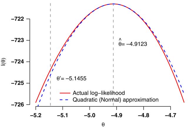
Figure 1 Log-likelihood in equation (4) with d=122 and E=16,586.3.
4. A One-Parameter Primer in Mis-Estimation Risk
4.1. Although θ is the parameter describing the mortality risk in section 3, actuaries have to value a monetary liability based on that risk. This can be described as a function of the risk parameter, say a(θ). a(θ) could be a valuation function for a single policy or, more usefully, the valuation of the liability for an entire portfolio. The best estimate of the liability in our simplistic mortality model would therefore be
 $$a(\hat{\theta })$$
. However, to allow for mis-estimation risk we would calculate something like
$$a(\hat{\theta })$$
. However, to allow for mis-estimation risk we would calculate something like
 $$a(\theta ')$$
, where θ′ was a stressed alternative value to
$$a(\theta ')$$
, where θ′ was a stressed alternative value to
 $$\hat{\theta }$$
which was less likely but nevertheless consistent with the observed data. For example, in Figure 1 an approximate 99.5% stress value for low mortality would be around θ′=5.1455 (see section 4.4 for derivation of θ′).
$$\hat{\theta }$$
which was less likely but nevertheless consistent with the observed data. For example, in Figure 1 an approximate 99.5% stress value for low mortality would be around θ′=5.1455 (see section 4.4 for derivation of θ′).
4.2. We can see from Figure 1 that the log-likelihood for θ is nearly quadratic and thus that
 $$\hat{\theta }$$
has an approximate Normal distribution. This means that we can generate alternative values to
$$\hat{\theta }$$
has an approximate Normal distribution. This means that we can generate alternative values to
 $$\hat{\theta }$$
which are consistent with the data by drawing values from a Normal distribution with mean
$$\hat{\theta }$$
which are consistent with the data by drawing values from a Normal distribution with mean
 $$\hat{\theta }$$
and variance
$$\hat{\theta }$$
and variance
 $$\hat{\sigma }^{2} $$
. In other words, we can generate
$$\hat{\sigma }^{2} $$
. In other words, we can generate
 $$\theta '\,{\equals}\,\hat{\theta }{\plus}\hat{\sigma }Z$$
, where Z represents a value from the cumulative distribution function for a N(0,1) variable,
$$\theta '\,{\equals}\,\hat{\theta }{\plus}\hat{\sigma }Z$$
, where Z represents a value from the cumulative distribution function for a N(0,1) variable,
 $$\Phi ()$$
. For finding a specific, consistent-but-stressed value for θ′ at a given p-value, we would calculate either
$$\Phi ()$$
. For finding a specific, consistent-but-stressed value for θ′ at a given p-value, we would calculate either
 $$Z\,{\equals}\,\Phi ^{{{\!\minus\!}1}} (p)$$
or
$$Z\,{\equals}\,\Phi ^{{{\!\minus\!}1}} (p)$$
or
 $$Z\,{\equals}\,\Phi ^{{{\!\minus\!}1}} (1{\minus}p)$$
, depending on whether increasing or decreasing θ raises or lowers the liability function, a(θ).
$$Z\,{\equals}\,\Phi ^{{{\!\minus\!}1}} (1{\minus}p)$$
, depending on whether increasing or decreasing θ raises or lowers the liability function, a(θ).
4.3. To illustrate this, assume that we want to value a temporary pension from age 60–65 years. The survival curve for our simple model is given by
 $$_{t} p_{{60}} \,{\equals}\,e^{{{\minus}te^{\theta } }} $$
. Ignoring discounting for simplicity, the valuation function for a continuously paid 5-year temporary annuity is given in the following equation:
$$_{t} p_{{60}} \,{\equals}\,e^{{{\minus}te^{\theta } }} $$
. Ignoring discounting for simplicity, the valuation function for a continuously paid 5-year temporary annuity is given in the following equation:
 $$a(\theta )\,{\equals}\,{{1{\minus}e^{{{\minus}5e^{\theta } }} } \over {e^{\theta } }}$$
4.4. In our example from section 3.4, the best-estimate liability is
 $$a(\hat{\theta })\,{\equals}\,a\,({\minus}\!4.9123)\,{\equals}\,4.9092$$
. If we then wanted to find the 99.5th percentile for mis-estimation risk, we would use
$$a(\hat{\theta })\,{\equals}\,a\,({\minus}\!4.9123)\,{\equals}\,4.9092$$
. If we then wanted to find the 99.5th percentile for mis-estimation risk, we would use
 $$Z\,{\equals}\,\Phi ^{{{\!\minus\!}1}} (0.005)\,{\equals}\,{\minus}2.5758$$
(Lindley & Scott, Reference Lindley and Scott1984, page 35), as lowering θ increases the liability. The value of the liability allowing for mis-estimation risk at the 99.5% level is then
$$Z\,{\equals}\,\Phi ^{{{\!\minus\!}1}} (0.005)\,{\equals}\,{\minus}2.5758$$
(Lindley & Scott, Reference Lindley and Scott1984, page 35), as lowering θ increases the liability. The value of the liability allowing for mis-estimation risk at the 99.5% level is then
 $$a(\hat{\theta }{\plus}\hat{\sigma }Z)\,{\equals}\,a\,({\minus}5.1455)\,{\equals}\,4.9279$$
, i.e. 0.38% higher than the central estimate. Our 99.5% allowance for mis-estimation risk would then be 0.38% of the best-estimate reserve.
$$a(\hat{\theta }{\plus}\hat{\sigma }Z)\,{\equals}\,a\,({\minus}5.1455)\,{\equals}\,4.9279$$
, i.e. 0.38% higher than the central estimate. Our 99.5% allowance for mis-estimation risk would then be 0.38% of the best-estimate reserve.
4.5. An implicit assumption in section 4.1 is that a(θ) is a monotonically increasing or decreasing function of θ (which is the case in equation (5)). If the liability function a(θ) is not simple or neatly behaved, then we can use simulation to generate values of Z. Specifically, we can repeatedly draw Z from the N(0,1) distribution, use Z to calculate θ′ and thus a(θ′), then add the value of a(θ′) to a set, S. We can then calculate the appropriate percentile of S as an estimate for the liability allowing for mis-estimation risk. A short R script for doing this with our simplistic temporary annuity example is given below:

which gives a value of 4.9275 for the 99.5th percentile, i.e. close to the analytical value in section 4.4. A more efficient estimate of the 99.5th percentile can be obtained by using the estimator from Harrell & Davis (Reference Harrell and Davis1982), as shown in the R script below:
which produces a value of 4.9278 for the 99.5th percentile, i.e. even closer agreement with the analytical approximation in section 4.4. In subsequent sections, we will see why correlations between parameters mean that, in most practical situations, we will invariably have to use the simulation approach of section 4.5. Appendix 3 considers methods for assessing mis-estimation risk which do not require large numbers of simulations.
4.6. In section 5, we will describe the general, multi-parameter case involving simulation, then in section 6 we will return to a simple two-parameter example for illustrative purposes.

5. The Multi-Parameter Case
5.1. We now assume a more realistic case where there are multiple parameters in a vector,
 $$\underline{{\mib{\theta }} } $$
. As in section 3, we have a log-likelihood function,
$$\underline{{\mib{\theta }} } $$
. As in section 3, we have a log-likelihood function,
 $$\ell (\underline{{\mib{\theta }} } )$$
, which we assume we can differentiate at least twice. The vector
$$\ell (\underline{{\mib{\theta }} } )$$
, which we assume we can differentiate at least twice. The vector
 $$\underline{{\mib{\theta }} } $$
is the analogue of the scalar θ in section 3, while the analogue of σ
2 is the variance–covariance matrix of
$$\underline{{\mib{\theta }} } $$
is the analogue of the scalar θ in section 3, while the analogue of σ
2 is the variance–covariance matrix of
 $$\underline{{\mib{\theta }} } $$
, say
V
. As in section 3.2, we have an unknown true parameter vector,
$$\underline{{\mib{\theta }} } $$
, say
V
. As in section 3.2, we have an unknown true parameter vector,
 $$\underline{{\mib{\theta }} } ^{{\bf {\asterisk}}} $$
, and an unknown true variance–covariance matrix,
V
*.
$$\underline{{\mib{\theta }} } ^{{\bf {\asterisk}}} $$
, and an unknown true variance–covariance matrix,
V
*.
5.2. Unlike in the one-parameter case in section 4.3, there is no easy analytical option to calculate the liability value allowing for mis-estimation. This is because the analogue of the scalar σ
2 in section 4.3 is a matrix,
V
, i.e. the parameters in
 $$\underline{{\mib{\theta }} } $$
will have various positive and negative correlations with each other. A visual example of this is given in Figure 4, where changing the value of the intercept (α
0) leads to a changed value for the slope (β
0). Thus, to assess the impact of mis-estimation risk we have to perform repeated valuations of the entire portfolio using a series of consistent alternative parameter vectors, analogous to the procedure in section 4.5. We repeat this process of valuation, which gives rise to a set, S, of portfolio valuations. S can then be used to set a capital requirement to cover mis-estimation risk. For example, Solvency II regime in the EU demands that this calculation takes place at the 99.5th percentile, and so the capital requirement would be given by the following formula:
$$\underline{{\mib{\theta }} } $$
will have various positive and negative correlations with each other. A visual example of this is given in Figure 4, where changing the value of the intercept (α
0) leads to a changed value for the slope (β
0). Thus, to assess the impact of mis-estimation risk we have to perform repeated valuations of the entire portfolio using a series of consistent alternative parameter vectors, analogous to the procedure in section 4.5. We repeat this process of valuation, which gives rise to a set, S, of portfolio valuations. S can then be used to set a capital requirement to cover mis-estimation risk. For example, Solvency II regime in the EU demands that this calculation takes place at the 99.5th percentile, and so the capital requirement would be given by the following formula:
 $$\left( {{{{\rm 99}{\rm .5}^{{{\rm th}}} \;{\rm percentile}\;{\rm of}\;S} \over {{\rm mean}\;{\rm of}\;S}}{\minus}1} \!\!\right){\times}100\,\%\,$$
5.3. The question then is how we generate those consistent alternative parameter vectors. To do this we use the same result from the theory of maximum likelihood as in section 3.2, which states that the joint estimate at the MLE is distributed as a multivariate Normal random variable with mean
 $$\underline{{\mib{\theta }} } ^{{\bf {\asterisk}}} $$
and a variance–covariance matrix,
V
* (Cox & Hinkley, Reference Cox and Hinkley1996, page 296). As in the one-parameter case, the true value of
$$\underline{{\mib{\theta }} } ^{{\bf {\asterisk}}} $$
and a variance–covariance matrix,
V
* (Cox & Hinkley, Reference Cox and Hinkley1996, page 296). As in the one-parameter case, the true value of
 $$\underline{{\mib{\theta }} } ^{{\bf {\asterisk}}} $$
is unknown, and so we substitute
$$\underline{{\mib{\theta }} } ^{{\bf {\asterisk}}} $$
is unknown, and so we substitute
 $$\underline{{{{\hat{\theta }}} }} $$
, the vector of MLE. We now seek a similar substitute for the unknown
V
*.
$$\underline{{{{\hat{\theta }}} }} $$
, the vector of MLE. We now seek a similar substitute for the unknown
V
*.
5.4. In some software packages, an estimated variance–covariance matrix is available directly. For example, in R (R Core Team, 2012) an estimate of
V
* is returned from using the vcov() function on a model object. However, actuaries often need to fit models which are unavailable in such software (Richards, Reference Richards2012), so it is useful to outline the general principle for estimating
V
* from knowledge of
 $$\ell (\underline{{\mib{\theta }} } )$$
alone.
$$\ell (\underline{{\mib{\theta }} } )$$
alone.
5.5. Let
 ${\scr H}(\underline{{\mib{\theta }} } )$
be the Hessian, i.e. the matrix of second-order partial derivatives of the log-likelihood function (McCullagh & Nelder, Reference McCullagh and Nelder1989, page 6). Let
${\scr H}(\underline{{\mib{\theta }} } )$
be the Hessian, i.e. the matrix of second-order partial derivatives of the log-likelihood function (McCullagh & Nelder, Reference McCullagh and Nelder1989, page 6). Let
 ${\scr I}\,{\equals}\,{\minus\!}{\scr H}(\underline{{{{\hat{\theta }}} }} )$
, i.e. the negative Hessian evaluated at the MLE
${\scr I}\,{\equals}\,{\minus\!}{\scr H}(\underline{{{{\hat{\theta }}} }} )$
, i.e. the negative Hessian evaluated at the MLE
 $$\underline{{{{\hat{\theta }}} }} $$
.
$$\underline{{{{\hat{\theta }}} }} $$
.
 ${\scr I}$
is the observed information matrix (sometimes also called the observed Fisher information). The diagonal elements of
${\scr I}$
is the observed information matrix (sometimes also called the observed Fisher information). The diagonal elements of
 ${\scr I}^{{{\!\minus}\!1}} $
are the Cramer–Rao lower bounds for the diagonal elements of
V
* (Cox & Hinkley, Reference Cox and Hinkley1996), and for practical purposes we substitute
${\scr I}^{{{\!\minus}\!1}} $
are the Cramer–Rao lower bounds for the diagonal elements of
V
* (Cox & Hinkley, Reference Cox and Hinkley1996), and for practical purposes we substitute
 ${\scr I}^{{{\!\minus}\!1}} $
for
V
*.
${\scr I}^{{{\!\minus}\!1}} $
for
V
*.
5.6. We thus have a multivariate Normal distribution for the MLE vector with mean
 $$\underline{{{{\hat{\theta }}} }} $$
and variance–covariance matrix
$$\underline{{{{\hat{\theta }}} }} $$
and variance–covariance matrix
 ${\scr I}^{{{\!\minus}\!1}} $
, i.e. MVN(
${\scr I}^{{{\!\minus}\!1}} $
, i.e. MVN(
 $\underline{{{{\hat{\theta }}} }} ,\,{\scr I}^{{{\!\minus}\!1}} $
) in place of MVN(
$\underline{{{{\hat{\theta }}} }} ,\,{\scr I}^{{{\!\minus}\!1}} $
) in place of MVN(
 $\underline{{\mib{\theta }} } ^{{\bf {\asterisk}}} ,\,{\mib{V}} ^{{\rm {\asterisk}}} $
). We can use this to simulate consistent vectors of alternative parameters as a means of investigating parameter risk and thus mis-estimation risk. To do this we calculate the expression in the following formula:
$\underline{{\mib{\theta }} } ^{{\bf {\asterisk}}} ,\,{\mib{V}} ^{{\rm {\asterisk}}} $
). We can use this to simulate consistent vectors of alternative parameters as a means of investigating parameter risk and thus mis-estimation risk. To do this we calculate the expression in the following formula:
 $$\underline{{{{\hat{\theta }}} }} {\plus}A\underline{{\mib{z}} } $$
where
 $$\underline{{\mib{z}} } $$
is a vector of independent, identically distributed N(0,1) variates with the same length as
$$\underline{{\mib{z}} } $$
is a vector of independent, identically distributed N(0,1) variates with the same length as
 $$\underline{{{{\hat{\theta }}} }} $$
. The matrix A represents the “square root” of
$$\underline{{{{\hat{\theta }}} }} $$
. The matrix A represents the “square root” of
 ${\scr I}^{{{\!\minus}\!1}} $
, of which there are generally several non-unique possibilities. However, the variance–covariance matrix
${\scr I}^{{{\!\minus}\!1}} $
, of which there are generally several non-unique possibilities. However, the variance–covariance matrix
 ${\scr I}^{{{\!\minus}\!1}} $
is a non-negative, definite matrix, and it is positive-definite apart from some trivial cases – see Lindgren (Reference Lindgren1976, page 464) for more details. We therefore set A to be the Cholesky decomposition of
${\scr I}^{{{\!\minus}\!1}} $
is a non-negative, definite matrix, and it is positive-definite apart from some trivial cases – see Lindgren (Reference Lindgren1976, page 464) for more details. We therefore set A to be the Cholesky decomposition of
 ${\scr I}^{{{\!\minus}\!1}} $
, i.e. A is a lower-triangular matrix such that
${\scr I}^{{{\!\minus}\!1}} $
, i.e. A is a lower-triangular matrix such that
 $AA^{T} \,{\equals}\,{\scr I}^{{{\!\minus}\!1}} $
– see Venables & Ripley (Reference Venables and Ripley2002, pages 62 and 422). From this we can use equation (7) to simulate parameter error consistent with the data, and thus use these perturbed parameter vectors to value the portfolio and explore mis-estimation risk.
$AA^{T} \,{\equals}\,{\scr I}^{{{\!\minus}\!1}} $
– see Venables & Ripley (Reference Venables and Ripley2002, pages 62 and 422). From this we can use equation (7) to simulate parameter error consistent with the data, and thus use these perturbed parameter vectors to value the portfolio and explore mis-estimation risk.
5.7. We then only require to calculate (i) the first derivatives of
 $$\ell $$
for finding the joint MLE, and (ii) the second partial derivatives to calculate
$$\ell $$
for finding the joint MLE, and (ii) the second partial derivatives to calculate
 ${\scr I}\!$
. These derivatives can be either worked out analytically or else approximated using finite differences. Appendix 2 considers these two approaches, and finds that analytical derivatives are strongly preferred for mis-estimation risk. We therefore use analytical derivatives throughout the main body of this paper.
${\scr I}\!$
. These derivatives can be either worked out analytically or else approximated using finite differences. Appendix 2 considers these two approaches, and finds that analytical derivatives are strongly preferred for mis-estimation risk. We therefore use analytical derivatives throughout the main body of this paper.
6. A Two-Parameter Case: The Importance of Acknowledging Correlations
6.1. In section 3, we had a simple one-parameter model behind the log-likelihood function, while the liability function in section 4 was not particularly realistic. In this section, we illustrate the calculation of mis-estimation risk for a pension paid throughout life and calibrate the mortality model using a wider age range from the pension scheme data in Appendix 1. Although the mortality model only contains two parameters, the example is sufficient to demonstrate the critical importance of acknowledging correlations between parameters when assessing mis-estimation risk.
6.2. We start by building
 $$\ell (\underline{{\mib{\theta }} } )$$
using a survival model for the force of mortality,
$$\ell (\underline{{\mib{\theta }} } )$$
using a survival model for the force of mortality,
 $$\mu _{x} $$
, which is defined in the following equation:
$$\mu _{x} $$
, which is defined in the following equation:
 $${ \mu _{x} \,{\equals}\, & \mathop {{\rm lim}}\limits_{h\to0^{{\plus}} } {1 \over h}{\rm Pr}\left( {{\rm death}\;{\rm before}\;{\rm age}\;x{\plus}h\!\mid\!{\rm alive}\;{\rm at}\;{\rm age}\;x} \right) \cr \,{\equals}\,\mathop {{\rm lim}}\limits_{h\to0^{{\plus}} } {{_{h} q_{x} } \over h} $$
and where the survival probability from age x to age x+t, t p x , is given by the following equation for any form of μ x :
 $$_{t} p_{x} \,{\equals}\,{\rm exp}\left( {{\!\!\minus}\!{\int}_0^t \mu _{{x{\plus}s}} ds} \right)$$
6.3. By using survival models we will therefore be modelling mortality at the level of the individual, rather than the group-level modelling of section 3. For further details of actuarial applications of survival models to pensioner and annuitant mortality the reader can consult Richards et al. (Reference Richards, Kaufhold and Rosenbusch2013).
6.4. In this section, we use a simple, two-parameter Gompertz (Reference Gompertz1825) model for each life in the following equation:
 $$\mu _{{x_{i} }} \,{\equals}\,e^{{\alpha _{0} {\plus}\beta _{0} x_{i} }} $$
6.5. The model in equation (10) is a simple model in age only, i.e. ignoring gender or any of the other known relevant risk factors (inclusion of other risk factors is considered in section 8). The results of fitting the model to the pension scheme experience data described in Appendix 1 are shown in Table 2, while Figure 2 shows the essentially quadratic profile of the log-likelihood for the two parameters. Note that we are applying a deliberately over-simple model to a fraction of the available data in order to reveal some important basic features. In section 8, we will make the model more realistic and practical.
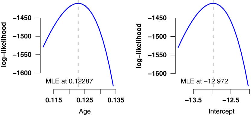
Figure 2 Log-likelihood profiles for model in Table 2. These profiles demonstrate the quadratic shape around the maximum likelihood estimates (MLEs), which is consistent with the multivariate Normal distribution for the estimates used in equation (7).
Table 2 Summary of Simple Gompertz (Reference Gompertz1825) Model Fitted to 2012 Mortality Experience of the Pension Scheme Described in Appendix 1

Data for ages 60 years and over, males and females combined.
Parameter significance is labelled according to the same scheme used in R (R Core Team, 2012), i.e. * for 5%, ** for 1% and *** for 0.1%.
6.6. Figure 3 shows the fitted mortality hazard from Table 2 against the crude mortality hazard for the pension scheme. We will not get sidetracked with questions of quality of fit or adequacy at this point, as our aim is to demonstrate mis-estimation risk. However, we note that section 8 introduces the concept of a financially suitable model as a critical foundation for assessing mis-estimation risk, together with a test for determining financial suitability.

Figure 3 log e (crude mortality hazard) and 95% confidence intervals for fitted model for ages 60 year and over. Data and model from Table 2. The crude mortality hazard is the actual number of deaths in the age interval [x,x+1) divided by the time lived in that interval.
6.7. In our model in Table 2 we have the MLEs
 $$\hat{\alpha }_{0} \,{\equals}\,{\!\minus}\!12.972$$
and
$$\hat{\alpha }_{0} \,{\equals}\,{\!\minus}\!12.972$$
and
 $$\hat{\beta }_{0} \,{\equals}\,0.122872$$
. If we define our MLE vector as
$$\hat{\beta }_{0} \,{\equals}\,0.122872$$
. If we define our MLE vector as
 $$\underline{{{{\hat{\theta }}} }} \,{\equals}\,(\hat{\beta }_{0} ,\hat{\alpha }_{0} )'$$
, then the estimated variance–covariance matrix using the approach defined in section 5.4 is as follows:
$$\underline{{{{\hat{\theta }}} }} \,{\equals}\,(\hat{\beta }_{0} ,\hat{\alpha }_{0} )'$$
, then the estimated variance–covariance matrix using the approach defined in section 5.4 is as follows:
 $$\matrix{ {\vskip18pt{\hat{\beta }_{0}} } \cr {\hat{\alpha }_{0} } \cr } \left(\!\! {\matrix{ {\matrix{ {\hat{\beta }_{0} } \cr {3.18189{\times}10^{{{\!\minus}\!5}} } \cr {{\!\minus}\!0.00261762} \cr } } & {\matrix{ {\hat{\alpha }_{0} } \cr {{\!\minus}\!0.00261762} \cr {0.218081} \cr } } \cr } } \!\!\right)$$
6.8. The correlation between
 $$\hat{\alpha }_{0} $$
and
$$\hat{\alpha }_{0} $$
and
 $$\hat{\beta }_{0} $$
is −99.4%
$$\hat{\beta }_{0} $$
is −99.4%
 $\left( {{\!\minus}\!99.4\,\%\,\,{\equals}\,{{{\!\minus}\!0.00261762} \over {\sqrt {3.18189{\times}10^{{{\!\minus}\!5}} {\times}0.218081} }}{\times}100\,\%\,} \!\right)$
(see Table 9 for further illustration of this). In other words, if
$\left( {{\!\minus}\!99.4\,\%\,\,{\equals}\,{{{\!\minus}\!0.00261762} \over {\sqrt {3.18189{\times}10^{{{\!\minus}\!5}} {\times}0.218081} }}{\times}100\,\%\,} \!\right)$
(see Table 9 for further illustration of this). In other words, if
 $$\hat{\alpha }_{0} $$
is mis-estimated then
$$\hat{\alpha }_{0} $$
is mis-estimated then
 $$\hat{\beta }_{0} $$
changes in the opposite direction by an almost perfectly known amount (and vice versa). This is illustrated in Figure 4, where we stress the intercept by 1.96 s.e. and re-estimate the age slope. Due to the strong correlation, a change in one parameter is accompanied by an important offsetting change in another. This is why a simple parallel shift in mortality table is not in general a correct statement of mis-estimation risk: the level of mortality (as represented by α
0) and the increase with age (as represented by β
0) are highly negatively correlated. A downward shift in level would result in an upward shift in the rate of increase by age, as shown in Figure 4. Mortality levels and rates of change by age are generally negatively correlated, as demonstrated later in Table 9, and this topic is explored in some detail for various risk factors in Richards et al. (Reference Richards, Kaufhold and Rosenbusch2013). Appendix 5 considers how to restructure a model to reduce parameter correlation, but this only works for the very simplest models. It is therefore important that any assessment of mis-estimation risk should acknowledge these correlations.
$$\hat{\beta }_{0} $$
changes in the opposite direction by an almost perfectly known amount (and vice versa). This is illustrated in Figure 4, where we stress the intercept by 1.96 s.e. and re-estimate the age slope. Due to the strong correlation, a change in one parameter is accompanied by an important offsetting change in another. This is why a simple parallel shift in mortality table is not in general a correct statement of mis-estimation risk: the level of mortality (as represented by α
0) and the increase with age (as represented by β
0) are highly negatively correlated. A downward shift in level would result in an upward shift in the rate of increase by age, as shown in Figure 4. Mortality levels and rates of change by age are generally negatively correlated, as demonstrated later in Table 9, and this topic is explored in some detail for various risk factors in Richards et al. (Reference Richards, Kaufhold and Rosenbusch2013). Appendix 5 considers how to restructure a model to reduce parameter correlation, but this only works for the very simplest models. It is therefore important that any assessment of mis-estimation risk should acknowledge these correlations.

Figure 4 log e (crude mortality hazard) with best-estimate fit and alternative line with stressed intercept (α 0) and re-estimated age slope (β 0). Ages 60 years and over, data and model from Table 2. The crude mortality hazard is the actual number of deaths in the age interval [x,x+1) divided by the time lived in that interval.
6.9. However, there are further consequences of the variance–covariance matrix in section 6.7, namely that the impact of mis-estimation risk varies by age. Figure 3 shows the 95% confidence interval for the fitted mortality hazard, which forms a bowed shape courtesy of the correlation in section 6.8. Within the model structure, the relative uncertainty is greatest at the youngest and oldest ends of the age range. The reason for this is that we are fitting a straight line, which must go through the data in the central age range. As a consequence, any mis-estimation of α 0 will cause a change in the estimation of β 0. As with a child’s see-saw, the change in fit near the centre will be much smaller than at either end. This same see-saw phenomenon will have major consequences for using multi-year data, as covered in section 7.
6.10. It is therefore important that any assessment of mis-estimation risk should acknowledge the age-related distribution of liabilities as well as the parameter correlations. To demonstrate this, assume that the liability function is for a single annuity at outset age x, i.e.
 $$a(\underline{{\mib{\theta }} } )$$
is defined as in the following equation:
$$a(\underline{{\mib{\theta }} } )$$
is defined as in the following equation:
 $${ a(\underline{{\mib{\theta }} } )\,{\equals}\, & \bar{a}_{x} \cr \,{\equals}\, & {\int}_0^\infty _{_t_} p_{x} v(t)dt $$
where v(t) is the continuous-time discount function. We use a constant net annual discount rate of 1% in this paper – UK government gilts with a maturity of 14–18 years yield around 3% at the time of writing and the Bank of England has a 2% inflation target (defined-benefit pensions in payment in the UK have compulsory indexation). However, it could also be argued that index-linked gilt yields are relevant for valuing pension scheme cashflows, and the yields for these are all negative at the time of writing. Using the model in Table 2, and a 1% net discount rate in the liability function in equation (11), the procedure described in section 4.5 yields the mis-estimation capital requirements shown in Figure 5. The mis-estimation capital required increases rapidly with age, which emphasises the importance of allowing for the age-related distribution of liabilities. The choice of discount rate (or yield curve) is obviously also important, as demonstrated in Figure 6, where a lower effective discount rate leads to a higher mis-estimation capital requirement.
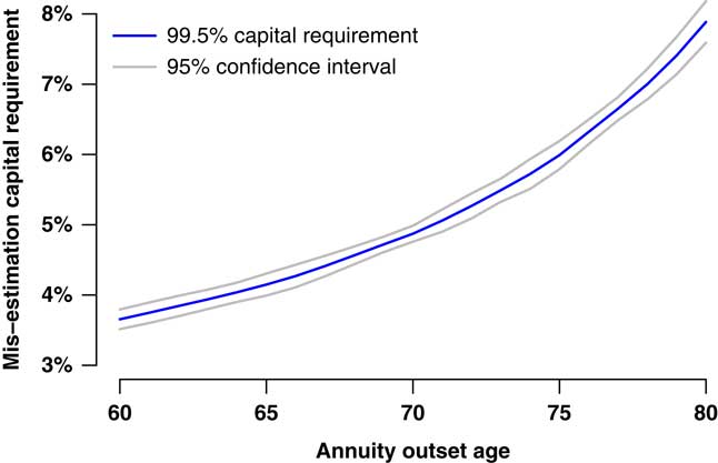
Figure 5 Mis-estimation risk capital requirement at 99.5% level as percentage of best-estimate reserve (with 95% confidence interval using Harrell & Davis (Reference Harrell and Davis1982) estimate). The liability is a single-level lifetime annuity from each stated age at outset, valued as in equation (11). Estimated from 10,000 simulations using model from Table 2 and discounting a level annuity at 1%/annum.
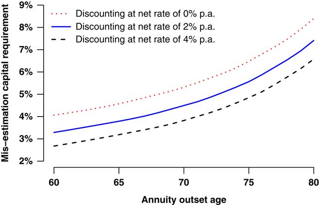
Figure 6 Mis-estimation risk capital requirement at 99.5% level as percentage of best-estimate reserve under various discount rates. The liability is a single-level lifetime annuity from each stated age at outset, valued as in equation (11). Estimated from 10,000 simulations using model from Table 2 with varying discount rates.
6.11. A selection of the mis-estimation capital requirements from Figure 5 is listed in Table 3. The average age of the 12,720 survivors at 1 January 2013 was 71.9 years (71.2 years weighted by annualised pension). Using a single model point would therefore suggest a mis-estimation capital requirement somewhere in the interval (4.90%, 5.22%).
Table 3 Specimen Mis-Estimation Capital Requirements from Figure 5 (95% Confidence Intervals Using the Method of Harrell & Davis (Reference Harrell and Davis1982), Calculated from 10,000 Valuations of a Single Annuity Discounted at a Net Rate of 1%/Annum)

6.12. However, it is doubtful whether a single model point, or even a handful of model points, can capture the impact of mis-estimation risk on an entire portfolio. It would obviously be more accurate to perform an entire portfolio valuation instead. This is relatively straightforward to do, and we therefore redefine the valuation function as in the following equation:
 $$a(\underline{{\mib{\theta }} } )\,{\equals}\,\mathop{\sum}\limits_{i\,{\equals}\,1}^n w_{i} \bar{a}_{{x_{i} }} $$
for all n survivors in the pension scheme. This automatically allows for not only the age distribution via the individual ages, x i , but also the liability distribution via the individual pensions, w i . Using the full-portfolio valuation function in equation (12) and the procedure in section 4.5 we get a 95% confidence interval for the mis-estimation capital of (4.57%, 4.90%). We can see that the range of mis-estimation capital requirements using the full-portfolio valuation is lower than would be implied by using a specimen model point at the average age and looking up Table 3. To show the impact of the distribution of the w i , setting all the pensions to the same value and redoing the full-portfolio valuation with section 4.5 yields a 95% confidence interval for the mis-estimation capital range of (4.64%, 5.00%). A full-portfolio valuation of individual liabilities yields a more accurate value for the mis-estimation capital requirement, which in this case also meant a lower requirement.
6.13. However, the model in Table 2 is implausibly simple: it does not contain enough relevant risk factors and only uses 1 year’s experience when more data are available. In section 8, we will fit models with more risk factors and consider other mortality laws, but we first need to consider the impact of using multi-year data.
7. The Impact of Using Multi-Year Data
7.1. The mis-estimation capital requirements in Figure 5 and Table 3 are based on only a single year’s mortality experience. In practice, most portfolios have experience data spanning several years, and this extra data contributes to improved estimation of parameters. This extra data also contributes to significantly reduced mis-estimation risk, as illustrated by comparing the first two rows in Table 4.
Table 4 99.5% Mis-Estimation Capital Requirements as Percentage of Best-Estimate Reserve

Results for various models and time periods calculated from 10,000 simulations. The 95% confidence intervals were calculated using the method of Harrell & Davis (Reference Harrell and Davis1982). Models calibrated using data for ages 60 years and over. For models including a time trend, the rates fitted are for 1 January 2010, i.e. µ x,2010.
7.2. However, an implicit assumption in the simple age-only model is that mortality is a stationary process in time. As many studies have shown, such as Willets (Reference Willets1999), mortality rates of pensioners and annuitants have been continuously falling for decades. We can allow for the fact that mortality is a moving target by including a time-trend parameter, δ, as in the following equation:
 $$\mu _{{x_{i} ,y}} \,{\equals}\,e^{{\alpha _{0} {\plus}\beta _{0} x_{i} {\plus}\delta (y{\!\minus}\!2000)}} $$
where µ x,y is the instantaneous force of mortality at exact age x and calendar time y. The offset of −2,000 keeps the parameters well scaled. The δ parameter could obviously be used to project mortality rates into the future as well as measuring the recent changes in mortality levels. However, we are concerned in this paper with mis-estimation risk of current rates, so to keep things comparable in Table 4, we generate static mortality rates as at 1 January 2010, i.e. using equation (13) the fitted rates used in the mis-estimation assessment will be µ x,2010.
7.3. One consequence of including this time-trend parameter is that it offsets a large part of the benefit of having the extra data, as shown in the third row of Table 4. This is an example of a phenomenon which occurs repeatedly with mis-estimation risk: enhancing the model’s fit can lead to an increase in mis-estimation risk. In the case of Table 4, there is little doubt that the model including time trend is a better fit: the Akaike information criterion (Akaike, Reference Akaike1987) is 15,801.3 with the time trend and 15,808.1 without it, while the log-likelihood profiles in Figure 7 confirm the validity of including each parameter as none of their plausible ranges includes 0. However, the better-fitting of the two models results in a higher mis-estimation capital requirement. Indeed, the inclusion of the time-trend parameter has added back over two-thirds of the reduction in mis-estimation capital requirements from the extra data.
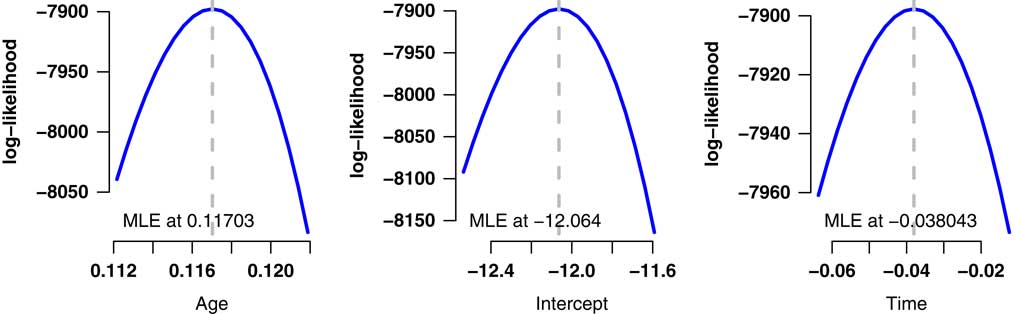
Figure 7 Log-likelihood profiles for Age+Time model in Table 4. These profiles demonstrate the quadratic shape around the maximum likelihood estimates (MLEs), which is consistent with the multivariate Normal distribution for the estimates in equation (7).
7.4. As this phenomenon might strike some readers as counter-intuitive, it is worth explaining it in more detail. At its heart we have the same see-saw phenomenon as in Figure 4, but here operating in calendar time. The time-trend parameter, δ, will be forced to pass through the “average” level of mortality across the period of observation, but it will be much less constrained at either end. This was the case in Figure 4 when looking at the behaviour of β 0 in response to changes in α 0. Thus, there is more uncertainty over the level of mortality at either end of the exposure period than there is over the mid-point of the period. In the presence of a time-varying mortality process, it is this see-saw effect which is offsetting much of the extra estimating power from using multi-year data.
7.5. This can be thought of more figuratively. Leaving aside the fact that mortality increases with age, if mortality were a static process in time then more experience data over a longer period of time will validly reduce mis-estimation risk. If there is no time trend, then the experience data of 5 years ago (say) will help inform you about mortality levels now: there is more relevant data on a process which is not changing in time. This is illustrated by comparing the first two rows of Table 4. However, if there is a time trend, then the experience data of 5 years ago is of less use in estimating current levels of mortality. While the time trend can be estimated, there is still uncertainty over its precise value, and it is this uncertainty which is undoing some of the benefit of the multi-year data. This is illustrated by comparing the last two rows of Table 4. Thus, where risk levels vary in time, as with pensioner and annuitant mortality, using experience data spanning multiple years will only yield modest reductions in mis-estimation risk. This is illustrated by comparing the first and last rows of Table 4. Other necessary improvements to the model will also increase the mis-estimation capital requirements, but for quite different reasons, and we will see why this is so in section 8.
8. A Minimally Acceptable Model for Financial Purposes
8.1. So far we have considered a simple two-parameter Gompertz model, which works well enough for ages above 60 years. However, Figure A1 shows an important amount of unused experience data in the age range 50–60 years, while Figure A2 shows that the data in this range will not fit the straight-line Gompertz assumption on a logarithmic scale. We solve this problem by using the mortality law in equation (14), which includes a constant component as per Makeham (Reference Makeham1860):
 $$\mu _{{x_{i} }} \,{\equals}\,{{e^{{\epsilon}} {\plus}e^{{\alpha _{0} {\plus}\beta _{0} x_{i} }} } \over {1{\plus}e^{{\alpha _{0} {\plus}\beta _{0} x_{i} }} }}$$
As before, we can also define a time-varying version of equation (14):
 $$\mu _{{x_{i} ,y}} \,{\equals}\,{{e^{{\epsilon}} {\plus}e^{{\alpha _{0} {\plus}\beta _{0} x_{i} {\plus}\delta (y{\!\minus}\!2000)}} } \over {1{\plus}e^{{\alpha _{0} {\plus}\beta _{0} x_{i} {\plus}\delta (y{\!\minus}\!2000)}} }}$$
8.2. The models in equations (14) and (15) do not allow for many risk factors, however. We can extend our model’s capabilities as follows:
 $$\mu _{{x_{i} ,y}} \,{\equals}\,{{e^{{\epsilon}} {\plus}e^{{\alpha _{0} {\plus}\mathop{\sum}{_{j} \alpha _{j} I_{{i,j}} {\plus}\beta _{0} x_{i} {\plus}\delta (y{\!\minus}\!2000)} }} } \over {1{\plus}e^{{\alpha _{0} {\plus}\mathop{\sum}{_{j} \alpha _{j} I_{{i,j}} {\plus}\beta _{0} x_{i} {\plus}\delta (y{\!\minus}\!2000)} }} }}$$
where α j represents the effect of risk factor j and I i,j is an indicator function taking the value 1 when life i possesses risk factor j and 0 otherwise. In this section, we will consider gender and pension size band as additional risk factors, but there is no practical limit to the number of risk factors which can be considered when modelling individual-level mortality. The benefits of individual- over group-level modelling are discussed in Richards et al. (Reference Richards, Kaufhold and Rosenbusch2013).
8.3. For a model to be useful for actuarial purposes we additionally require that all financially significant risk factors are included. To test whether a model achieves this we use the process of bootstrapping described in Richards et al. (Reference Richards, Kaufhold and Rosenbusch2013), i.e. we sample from the data and calculate the ratio of the actual number of deaths in the sample to the predicted number according to the model. The results of this are shown for two models in Table 5, where the ratios for the lives column are close to 100%. This means that both models have a good record in predicting the number of deaths, as one would expect for models fitted by the method of maximum likelihood. However, we can see that the model in the first row has a poor record when the ratio is weighted by pension size. This is because those with larger pensions have a lower mortality rate, thus leading the first model to over-state pension-weighted mortality. The first model in Table 5 is therefore unacceptable for financial purposes.
Table 5 Bootstrapping Results for Two Alternative Models

Calibrated to 2007–2012 mortality experience of pension scheme described in Appendix 1 (ages 50 years and over). Bootstrap sample size is 1,000 (sampling with replacement) and 1,000 samples are taken. Mortality rates are as at 1 January 2013, i.e. we are using µ x,2013 without projection. Model notation follows that of Baker & Nelder (Reference Baker and Nelder1978).
8.4. The second row in Table 5 shows that the addition of a three-level risk factor for pension size makes a material improvement in the amounts-weighted bootstrap ratio. Although the median bootstrap ratio is not quite as close to 100% as we might like, it is a clear improvement on the first model and could therefore be regarded as a minimally acceptable model for financial purposes. We can also see that the inclusion of a necessary risk factor (pension size) has increased the capital requirement for mis-estimation risk. The reason for this is the concentration of risk demonstrated in Table A2 – the bulk of the total pension is paid to a small proportion of the overall lives, yet these same lives experience lower mortality rates, as shown in Table 6. In effect, the liability of the scheme is driven by a much smaller effective number of lives than a simple headcount would imply, and the mortality level of these lives is lower. This concentration of risk makes it very important that (i) the model reflects these dynamics, and (ii) that the mis-estimation valuation function
 $$a(\underline{{\mib{\theta }} } )$$
reflects the impact of these lives. Using a valuation function which performs a valuation of the whole portfolio will do this.
$$a(\underline{{\mib{\theta }} } )$$
reflects the impact of these lives. Using a valuation function which performs a valuation of the whole portfolio will do this.
Table 6 Summary of Age+Gender+Makeham+Time+Size Model Using Equation (16)

Calibrated using experience data for ages 50 years and over. Parameter significance is labelled according to the same scheme used in R (R Core Team, 2012), i.e. * for 5%, ** for 1% and *** for 0.1%.
8.5. In practice, an actuary would use a more sophisticated model than the one in Table 6. Risk factors like gender and pension size would normally be allowed to vary by age, for example, and most portfolios have scope for additional rating factors such as early retirement indicators or postcode-based profiling – see Richards (Reference Richards2008) for further details (Figure 8).
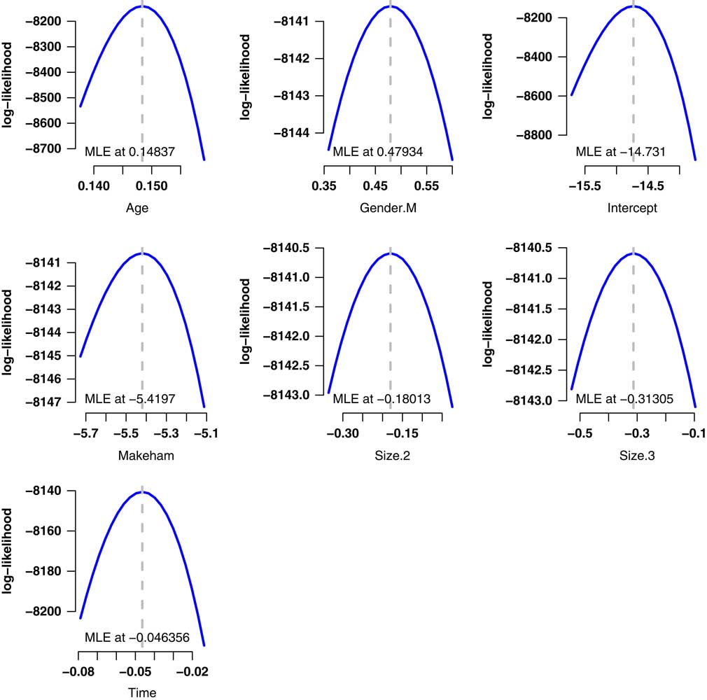
Figure 8 Log-likelihood function in profile for each of the seven parameters in Table 6, showing the essentially quadratic nature of the function, and thus the validity of the multivariate normal assumption in section 5.3.
9. Discussion
9.1. Before using the mis-estimation method described in this paper, it is important that the analyst check three items. The first requirement is that the independence assumption must hold: data must be deduplicated and the model must be well specified. Data with duplicates will give a falsely low estimate of mis-estimation risk, but a bigger risk comes from badly specified models. One example is the still-encountered practice of chopping up the experience of individuals into non-overlapping annual pieces and fitting a q x model with a generalised linear model. Such models will understate mis-estimation risk capital if applied in the manner described in this paper.
9.2. The second requirement is that the model allows for all financially significant risk factors. A model which does not contain these will give an erroneously low estimate of mis-estimation risk, as illustrated in Table 5. This is because the financial impact of each life is not the same – those with larger pensions have a much larger influence than those with smaller pensions. This is compounded by the fact that those with larger pensions usually live longer, as shown by the lower mortality of the Size.3 group in Table 6. Thus, both the overall reserves and the associated mis-estimation risk are largely driven by a small proportion of the overall portfolio membership. The bootstrapping procedure of section 8.3 can test whether a model has included all financially relevant risk factors.
9.3. The third requirement for multi-year data is to check that the model includes a time-trend parameter, if one is needed. An additional useful check is that the log-likelihood function is approximately quadratic around each MLE, i.e. that the multivariate Normal assumption behind Formula 7 holds.
9.4. Mis-estimation risk is portfolio dependent. Different portfolios, and models with different risk factors, will produce different mis-estimation capital requirements. By and large, the more experience data there is, the lower the mis-estimation risk will be. We can illustrate this by using a large population of German pensioners. A comparison of the scale of the data sets is given in Table 7, where the German data set is a factor of around 15 times larger.
Table 7 Comparison of UK Pension Scheme from Appendix 1 and a German Pensioner Population

9.5. A comparison of Tables 5 and 8 shows that the same minimally acceptable model does a reasonable – but not perfect – job of explaining financially weighted mortality variation in the UK scheme and amongst the German pensioners. However, although the German data set is around 15 times larger, the mis-estimation capital requirement is only reduced by three quarters.
Table 8 Bootstrapping Results for German Pensioner Data

Calibrated to 2007–2011 mortality experience of pension scheme described in Richards et al. (Reference Richards, Kaufhold and Rosenbusch2013) (ages 50 years and over). Bootstrap sample size is 1,000 (sampling with replacement) and 1,000 samples are taken. Mortality rates are as at 1 January 2012, i.e. we are using µ x,2012 without projection. Model notation follows that of Baker & Nelder (Reference Baker and Nelder1978).
9.6. More data can come from the portfolio being larger or from a longer exposure period, although the benefit of multi-year data is tempered when a time trend exists. The mis-estimation capital requirements also vary according to the discount rate or yield curve, as shown in Figure 6, so such calculations will need to be regularly updated as the interest rate environment changes.
9.7. The capital requirements produced by this method should also be taken as a lower bound, and actuarial judgement will need to be applied as to the extent of any additional allowances which might be necessary. For example, if a portfolio were growing quickly, a larger addition would be needed than if the portfolio were growing slowly. A still-larger adjustment might be required if the portfolio were growing due to a new business source. For example, consider a life office that historically wrote internal vesting annuities, but then made a decision to write open-market annuities or bulk-purchase annuities. This would create extra mis-estimation risk that could not be captured in a procedure calibrated using only the internal-vesting mortality experience. Such circumstances would require additional capital to be held for mis-estimation risk, and this can only be determined by actuarial judgement.
9.8. We note also that a matrix of correlations between parameters, C, can be derived from the variance–covariance matrix, V, by setting
 $c_{{i,j}} \,{\equals}\,v_{{i,j}} \!/\!\sqrt {v_{{i,i}} v_{{j,j}} } $
, where c
i,j
and v
i,j
are the values in row i and column j of the matrices C and V, respectively. C is symmetric around the leading diagonal, as is V, and the leading diagonal of C is composed of 1s, as each parameter is perfectly correlated with itself. All entries in C lie between −1 and +1 (which represent perfect negative and perfect positive correlation, respectively). An example of correlation matrix is given in Table 9, calculated according to the steps outlined above.
$c_{{i,j}} \,{\equals}\,v_{{i,j}} \!/\!\sqrt {v_{{i,i}} v_{{j,j}} } $
, where c
i,j
and v
i,j
are the values in row i and column j of the matrices C and V, respectively. C is symmetric around the leading diagonal, as is V, and the leading diagonal of C is composed of 1s, as each parameter is perfectly correlated with itself. All entries in C lie between −1 and +1 (which represent perfect negative and perfect positive correlation, respectively). An example of correlation matrix is given in Table 9, calculated according to the steps outlined above.
Table 9 Percentage Correlations Between Coefficients in the Model from Table 6, i.e. c i,j ×100%

As with the variance–covariance matrix, the correlation matrix is symmetric about the leading diagonal. The leading diagonal is 100% because a parameter value is perfectly correlated with itself.
9.9. One item worth noting in Table 9 is that the time-trend parameter has little correlation with any parameter apart from the intercept, with which it is negatively correlated. This is different from the model for the German pensioner data set in Richards et al. (Reference Richards, Kaufhold and Rosenbusch2013), where the time-trend parameter was not strongly correlated with any of the other parameters. This has potential application to the correlation matrix used by insurers when allowing for diversification of risks under the Solvency II regime. The correlation between the time-trend parameter and the others could be used to support the assumed correlation between mis-estimation risk and mortality improvements. This would have to be assessed on a portfolio-by-portfolio basis, however, and would require actuarial judgement. In the case of this portfolio, however, the negative correlation between the time trend and the intercept could perhaps be used to justify a negative correlation between mis-estimation risk and trend risk. If so, this would bring an overall indirect capital benefit from using multi-year data, despite the modest reduction in mis-estimation capital in section 7 from including a time trend in the model.
10. Conclusions
10.1. Mis-estimation risk for a portfolio can be straightforwardly assessed using the portfolio’s own experience data and some basic results for MLEs. An approximation for the variance–covariance matrix is required, but this can be quickly derived from the log-likelihood function for any statistical model. Increased portfolio size leads to better estimation and thus lower mis-estimation capital requirements, but section 9 shows that there is a diminishing return. Similarly, experience data spanning multiple years provide only a modest reduction in mis-estimation capital requirements where risk rates are changing in time, as shown in section 7. However, larger portfolio size or a longer exposure period could bring indirect capital benefits from examining the matrix of parameter correlations, as in section 9.9.
10.2. Parameters estimated from any statistical model are correlated to some extent, and these correlations need to be acknowledged in assessing mis-estimation risk. Furthermore, uncertainty over fitted rates varies by age and some of the greatest parameter uncertainty applies to the lives with the largest concentration of liabilities. The concentration of liabilities in a small subset of lives is one reason why an improved model fit can lead to higher mis-estimation risk. A full-portfolio valuation using appropriately perturbed model parameters will therefore allow for all of these aspects when assessing mis-estimation risk.
Acknowledgements
The author thanks Gavin P. Ritchie, Dr Shane F. Whelan, Dr Iain D. Currie, Dr Matthias Börger, Professor Andrew J. G. Cairns and Kai Kaufhold for helpful comments. Data validation and preparation for modelling were done using Longevitas (Longevitas Development Team, 2014), which was also used to fit all the models and assess mis-estimation risk. Graphs were done in R (R Core Team, 2012). Any errors or omissions remain the sole responsibility of the author.
11. Appendix 1: Details of Scheme Used to Illustrate Results
11.1. The data used to illustrate results in this paper are for a medium-sized, local-authority pension scheme in England and Wales. The data fields available were as follows: date of birth, gender, commencement date, total annual pension, end date, postcode, National Insurance number and whether the pensioner was a child, retiree or widow(er). The end date was determined differently for deaths, temporary pensions and survivors to the extract date. For deaths, the end date was the date of death. For children’s pensions and trivial commutations, the end date was the date the pension ceased or was commuted. For other survivors, the end date was the date of extract in early 2013. The experience data beyond 31 December 2012 were not used to avoid bias from delays in death reporting.
11.2. There were 17,068 benefit records available before deduplication, of which one was rejected for having an end date inconsistent with the commencement date. Of the remaining 17,067 records, 2,265 were marked as deaths.
11.3. Annuitants and pensioners often have multiple benefit records. It is particularly common in annuity portfolios for people to have multiple annuities, as demonstrated in Richards (Reference Richards2008). The phenomenon is less common for pension schemes, but multiple benefit records for the same individual can still arise. The first scenario is where an individual accrues two or more benefits from separate periods of service. The second scenario is where an individual receives a pension in respect of their own service and also a spouse’s pension if they were a widow(er) of a deceased pensioner in the same scheme. Administratively, it is usually easier to handle these multiple benefits separately, even though they are paid to the same person, and so duplicate records arise.
11.4. It is essential in any statistical model that the assumption of independence is valid, so we must perform deduplication, i.e. the identification of individuals with multiple benefit records. Following Richards (Reference Richards2008) we use two different deduplication schemes based on matching individual data items on each record. Each matching rule forms a deduplication key based on verified data items; if all items of the deduplication key match, then the two or more matching records are merged and the pension amounts added together. The details of this procedure are summarised in Table A1. The two records with conflicting life statuses were rejected, leaving 16,131 records (16,131=17,068−1−934−2).
Table A1 Deduplication Results for Medium-Sized Pension Scheme in England and Wales

11.5. The number of duplicates may seem modest in relation to the overall number of records, but it is important to deduplicate for a number of reasons. For example, if an individual received two pensions of £4,000 each, this should be recognised as one individual in group S09 in Table A2 and not two records in group S07. Failure to deduplicate leads to bias in mortality models and to falsely comforting estimates of parameter variance, and thus under-statement of mis-estimation risk. The resulting data volumes are shown in Figure A1.
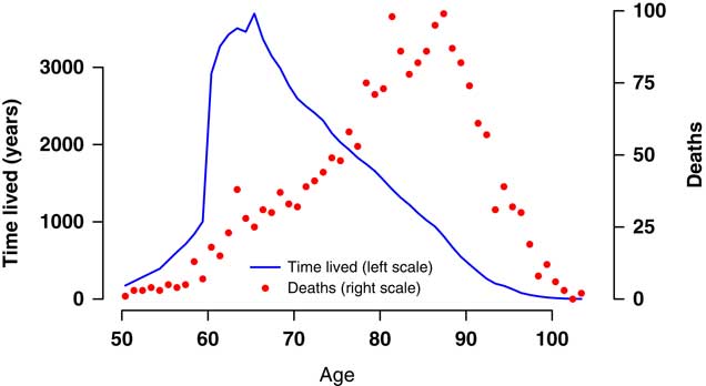
Figure A1 Deaths and time lived at ages 50 years and over for 2007–2012, males and females combined. In the given age and date range there were 2,076 deaths among 15,698 lives, with a total exposure time of 71,162.93 years. Exposure time and deaths before 1 January 2007 were not used and exposure times and deaths after 31 December 2012 were discarded to reduce the influence of delays in death reporting.
Table A2 Data by Pension Size Band

11.6. One issue with pension schemes is that pensions are usually increased from year to year. This creates a bias problem for cases which terminate early, i.e. deaths and temporary pensions. To put all pension values on the same approximate financial footing, therefore, the annual pension amounts for early terminations were revalued by 2.5%/annum to the end of the period of observation (the Retail Price Index increased by a geometric average of 2.68% over this period, while the Consumer Price Index increased by 2.90%). A more accurate approach would have been to establish the actual scheme increases over the period, together with their timing and split between different types of benefits. However, this level of detail would not have made any material change to the results in this paper.
11.7. Table A2 shows the breakdown of the deduplicated data by revalued annual pension. The pension scheme shows considerable concentration of risk, as the top 20% of lives account for 58.7% of the total pension. This phenomenon is common in the United Kingdom, as demonstrated for other portfolios in Richards (Reference Richards2008).
11.8. Figure A2 shows the crude mortality hazard on a logarithmic scale for males and females combined. There is no obvious evidence of a data problem, with the mortality hazard approximately log-linear above age 60 years. A further useful check on the validity of the data is to plot the Kaplan–Meier curves (Kaplan & Meier, Reference Kaplan and Meier1958). We have encountered other portfolios where there is not a clear separation between survival curves for males and females. This is sometimes evidence of a data-corruption problem, which can be related to the processing of benefits for surviving spouses. However, Figure A3 shows that females have a consistently higher probability of reaching any given age, leading us to conclude that the data here do not suffer from any obvious corruption. Table A3 contains the mortality ratios for the deduplicated scheme data, which suggest falling mortality levels with a large degree of volatility in the annual experience.
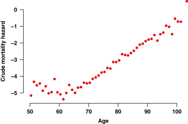
Figure A2 Crude mortality hazard for males and females combined in medium-sized UK pension scheme. Data cover ages 50 years and over for the period 2007–2012. The crude mortality hazard is the actual number of deaths in the age interval [x,x+1) divided by the time lived in that interval. The falling mortality rate over the age range 50–60 years is caused by excess mortality from ill-health retirements (the gender mix in this age range is broadly constant, with females accounting for variable 42%–53% of exposure at individual ages).
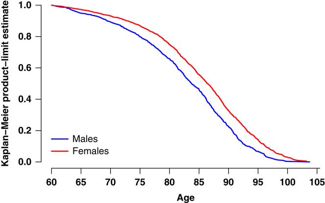
Figure A3 Kaplan–Meier product-limit estimate from age 60 years for males and females in medium-sized UK pension scheme. The data cover ages 60 years and over in the period 2007–2012. The version of the Kaplan–Meier estimate plotted is that defined in Richards (Reference Richards2012).
Table A3 Actual Deaths Against S2PA Without Adjustment, Weighted by Lives and Revalued Pension Amounts

12. Appendix 2: Analytical Derivatives Versus Numerical Approximations
12.1. When fitting mortality models, the foundation of modern statistical inference is the log-likelihood function,
 $$\ell $$
. The point at which the log-likelihood has its maximum value gives you the joint MLEs of the parameters, while the curvature of the log-likelihood gives information about the uncertainty of those parameter estimates. The key to both is the calculation of derivatives: gradients (first derivatives) for maximising the log-likelihood function and curvature (second partial derivatives) for estimating the variance–covariance matrix. In each case, we require either the analytical derivatives themselves, or else numerical approximations of them.
$$\ell $$
. The point at which the log-likelihood has its maximum value gives you the joint MLEs of the parameters, while the curvature of the log-likelihood gives information about the uncertainty of those parameter estimates. The key to both is the calculation of derivatives: gradients (first derivatives) for maximising the log-likelihood function and curvature (second partial derivatives) for estimating the variance–covariance matrix. In each case, we require either the analytical derivatives themselves, or else numerical approximations of them.
12.2. Numerical approximations to derivatives can be obtained relatively straightforwardly by using difference quotients. This involves perturbing a parameter by a small value, say h, and then expressing the change in function value relative to h. For example, a central difference quotient of the single-parameter log-likelihood function,
 $$\ell (\theta )$$
, will yield a numerical approximation of the first derivative, as in the following equation:
$$\ell (\theta )$$
, will yield a numerical approximation of the first derivative, as in the following equation:
 $${{\partial \ell } \over {\partial \theta }}\,\approx\,{{\delta _{h} [\ell ](\theta )} \over h}\,{\equals}\,{{\ell (\theta {\plus}h\,/\,2){\!\minus}\!\ell (\theta {\!\minus}\!h\!/\!2)} \over h}$$
and a similar central difference quotient can be used to approximate the second derivative, as in the following equation:
 $${{\partial ^{2} \ell } \over {\partial \theta ^{2} }}\,\approx\,{{\delta _{h}^{2} [\ell ](\theta )} \over {h^{2} }}\,{\equals}\,{{\ell (\theta {\plus}h){\!\minus}\!2\ell (\theta ){\plus}\ell (\theta {\!\minus}\!h)} \over {h^{2} }}$$
12.3. For the multi-parameter case, equation (A1) must be applied to each parameter in turn, with the other parameters unperturbed. A simple extension of equation (A2) is used for second partial derivatives. In theory, the smaller the value of h, the closer the numerical approximation will be to the actual derivative. Such numerical approximations have the advantage that they avoid the need to work out large numbers of analytical derivatives for each mortality law. However, there are drawbacks in terms of stability and accuracy, and this is most evident for estimating the curvature. By way of illustration, Table A4 shows the estimates and approximate standard errors for one of the parameters in a simple two-parameter Gompertz model using numerical approximations for the derivatives.
Table A4 Estimated Value and Approximate Standard Error for the Intercept (
 $$\hat{\alpha }_{0} $$
) Parameter in the Simple Gompertz Model for Mortality in Table 2
$$\hat{\alpha }_{0} $$
) Parameter in the Simple Gompertz Model for Mortality in Table 2

12.4. The MLE of the intercept parameter in Table A4 is consistent to five significant figures for values of h=10−4 and smaller, with a degree of convergence apparently achieved for values of h=10−5 and smaller. However, there is no such obvious convergence for the approximate standard error, with the estimate becoming unstable for very small values of h. This is not an isolated result – similar work with other schemes and other models produces the same finding. Furthermore, although the value of h=10−4 looks like the best compromise in Table A4, this is not the case for other models and other data sets. Our conclusion therefore is that while numerical approximations are often fine for finding the MLEs, they are not reliable enough for estimating the variance–covariance matrix.
12.5. For reliability one simply has to do the maths and find the expressions for the analytical derivatives. This has the additional advantage that points of possible arithmetic underflow can be identified and handled – see Richards (Reference Richards2012) for a list of some problematic expressions and how to cope with them. Another advantage is that using the analytical derivatives typically results in faster fitting times. Using analytical derivatives the values for the parameters in Table A4 are −12.972 for the intercept and 0.467 for s.e. (see Table 2). From this we can deduce that h=10−4 was indeed the best-performing approximation step in Table A4. There is of course a degree of irony in having to calculate the analytical derivatives to find out which numerical approximation performs best – one might as well just use the analytical derivatives. However, it is useful to be able to do both as a means of checking one’s mathematics.
12.6. The methodology in this paper requires the accurate estimation of the variance–covariance matrix, which we estimate from the inverted matrix of second partial derivatives. The best way to accurately estimate the latter is to work out the analytical derivatives. This is admittedly more work than using difference quotients like equations (A1) and (A2), but, as demonstrated in Table A4, using analytical derivatives is the most reliable way to fit the model parameters and to estimate their variance–covariance matrix.
13. Appendix 3: Number of Simulations Required
13.1. In the main body of this paper we used 10,000 simulations of equation (7), followed by full-portfolio valuations in section 8. The simulations can be done quickly enough, but the portfolio valuations which accompany them can be computationally demanding. It is worth commenting on two practical methods to speed things up.
13.2. The first method is to exploit the fact that each simulation in equation (7) is independent of all the others, as are the associated portfolio valuations. We can therefore use parallel processing to perform the same work in a much shorter period of time. The mis-estimation algorithm in this paper is highly scaleable, i.e. spreading the work over u CPUs means the work can be done in
 $${1 \over u}$$
of the elapsed time. This was the method adopted for this paper, where calculations were spread over seven CPUs.
$${1 \over u}$$
of the elapsed time. This was the method adopted for this paper, where calculations were spread over seven CPUs.
13.3. The second method is to see whether there is an appropriate distributional assumption which can be made for the portfolio valuations in S (as defined for equation 6). The number of simulations could be curtailed if it were found that the values in S followed, say, a Normal distribution, as the mean and variance could be robustly estimated and all higher-order moments are a function of these. This approach was considered by Richards et al. (Reference Richards, Currie and Ritchie2014), where the much larger number of parameters in projection models – and the greater variance in the estimates – made an approach like equation (7) trickier. However, the distribution of the values in the resulting set S in Richards et al. (Reference Richards, Currie and Ritchie2014) was only Normally distributed for a subset of projection models, so this second method could not be universally used. That said, the mis-estimation approach in equation (7) is very different and the number of parameters is much smaller, so it is worth considering if this second method might apply here.
13.4. The Normal distribution is fully characterised by its mean and variance, i.e. the first two moments of the distribution. Higher-order moments are merely a function of the first two. In general, if a distribution has mean µ, then the coefficient of skewness (standardised third moment) is given by the following formula:
 $${{E(s{\!\minus}\!\mu )^{3} } \over {[E(s{\!\minus}\!\mu )^{2} ]^{{{3 \over 2}}} }}$$
where E denotes expectation – see Wetherill (Reference Wetherill1982, page 88). Formula A3 is zero for the Normal distribution. Similarly, adjusting the coefficient of kurtosis (standardised fourth moment) given in Wetherill (Reference Wetherill1982, page 88) we get the following formula:
 $${{E(s{\!\minus}\!\mu )^{4} } \over {[E(s{\!\minus}\!\mu )^{2} ]^{2} }}$$
which is 3 for the Normal distribution. Thus, if the skewness coefficient of the data in S is close to 0 and the kurtosis coefficient of the same data is close to 3, then it would be appropriate to use the Normal distribution as a means of finding the percentiles of S. The skewness and kurtosis of the valuations in S for the models used in the main body of this paper are given in Table A5. For comparison we also show the skewness and kurtosis of 10,000 simulations from the N(0,1) distribution using the R script below:
Table A5 Skewness and Kurtosis of Portfolio Valuations and simulated N(0,1) variates


13.5. The results in Table A5 show that the portfolio valuations in S have a skewness close to 0 and a kurtosis close to 3. In each case the distribution of S can therefore be closely approximated by a Normal distribution. Thus, for these models and this particular portfolio at least, one could calculate the mis-estimation capital requirements from the mean and standard deviation of S, together with the appropriate value of
 $$\Phi ^{{{\!\minus}\!1}} ()$$
. Indeed, one could arguably use far fewer than 10,000 simulations, as the mean and standard deviation of Normally distributed data can be reliably estimated with fewer data points.
$$\Phi ^{{{\!\minus}\!1}} ()$$
. Indeed, one could arguably use far fewer than 10,000 simulations, as the mean and standard deviation of Normally distributed data can be reliably estimated with fewer data points.
14. Appendix 4: Conversion to Published Tables
14.1. It is one thing to be able to fit a bespoke model with multiple risk factors. However, actuaries also need to express their bespoke bases in terms of a published table for communication purposes. Examples include reserving bases, communication with third parties (such as regulators and auditors) and of course circumstances where one wants to keep one’s bespoke basis private (as in competitive pricing).
14.2. A good way to convert mortality bases is by equating reserves, the so-called “equivalent-annuity method” – see Willets (Reference Willets1999) and Richards et al. (Reference Richards, Kaufhold and Rosenbusch2013) for examples. This involves solving an equation where the only difference on each side is the mortality basis being used. For example, two mortality bases B and T would be deemed equivalent for a given annuity portfolio if the following equation held:
 $$\mathop{\sum}\limits_{i\,{\equals}\,1}^n w_{i} \ddot{a}_{{x_{i} }}^{T} \,{\equals}\,\mathop{\sum}\limits_{i\,{\equals}\,1}^n w_{i} \ddot{a}_{{x_{i} }}^{B} $$
where w
i
is the annual pension paid to life i and
 $$\ddot{a}_{{x_{i} }} $$
values an immediate level lifetime annuity paid to a life aged x
i
. Without loss of generality we can think of B as the bespoke, multi-factor basis and T as the much simpler one based on the published table. In the case of gender-differentiated rates in T, which is usually the norm, equation (A5) is generally applied separately to males and females. For example, the equivalent percentages of S2PA (CMI Ltd., 2014) for the model in Table 6 are given in the first row of Table A6, where the values are consistent with the 2012 column of Table A3.
$$\ddot{a}_{{x_{i} }} $$
values an immediate level lifetime annuity paid to a life aged x
i
. Without loss of generality we can think of B as the bespoke, multi-factor basis and T as the much simpler one based on the published table. In the case of gender-differentiated rates in T, which is usually the norm, equation (A5) is generally applied separately to males and females. For example, the equivalent percentages of S2PA (CMI Ltd., 2014) for the model in Table 6 are given in the first row of Table A6, where the values are consistent with the 2012 column of Table A3.
14.3. Alternatively, the actuary can solve for a target reserve value, as in the following equation:
 $$\mathop{\sum}\limits_{i\,{\equals}\,1}^n w_{i} \ddot{a}_{{x_{i} }}^{T} \,{\equals}\,S^{p} $$
where S
p
would be the appropriate percentile of the set of mis-estimation valuations carried out with similar
 $$\ddot{a}$$
functions. For example, an approximate 95% confidence interval for the best-estimate basis could be obtained by solving for S
2.5% and S
97.5%. This is done in the second row of Table A6, where we note that the confidence interval is not symmetric around the best-estimate percentages. One important point to note is that for gender-differentiated rates we would have to solve equation (A6) separately for males and females. Alternatively, we could solve for the aggregate male and female reserves combined and use the same percentage of table for both genders. Bearing in mind the similar percentages for males and females in Table A6, this would be an option here.
$$\ddot{a}$$
functions. For example, an approximate 95% confidence interval for the best-estimate basis could be obtained by solving for S
2.5% and S
97.5%. This is done in the second row of Table A6, where we note that the confidence interval is not symmetric around the best-estimate percentages. One important point to note is that for gender-differentiated rates we would have to solve equation (A6) separately for males and females. Alternatively, we could solve for the aggregate male and female reserves combined and use the same percentage of table for both genders. Bearing in mind the similar percentages for males and females in Table A6, this would be an option here.
14.4. Finally, we can also express our 99.5% mis-estimation stress in terms of a standard table by using S 99.5% in equation (A6). This is given in the third row of Table A6. One reason for doing this might be if one needed a rough-and-ready approximation for daily stress testing.
15. Appendix 5: Orthogonality and Parameter Correlation
15.1. In section 6.8, we noted a high correlation between the estimates of the intercept (
 $$\hat{\alpha }_{0} $$
) and age parameter (
$$\hat{\alpha }_{0} $$
) and age parameter (
 $$\hat{\beta }_{0} $$
). In the case of the simple two-parameter Gompertz model, this is a direct result of the choice of parameterisation in equation (10). However, we can attempt to orthogonalise
$$\hat{\beta }_{0} $$
). In the case of the simple two-parameter Gompertz model, this is a direct result of the choice of parameterisation in equation (10). However, we can attempt to orthogonalise
 $$\hat{\alpha }_{0} $$
and
$$\hat{\alpha }_{0} $$
and
 $$\hat{\beta }_{0} $$
by re-parameterising the model as in the following equation:
$$\hat{\beta }_{0} $$
by re-parameterising the model as in the following equation:
 $$\mu _{{x_{i} }} \,{\equals}\,e^{{\alpha _{0} {\plus}\beta _{0} (x_{i} {\!\minus}\!o)}} $$
where o is an offset constant. In a model for grouped mortality counts, Cairns et al. (Reference Cairns, Blake and Dowd2006) used
 $$o\,{\equals}\,\bar{x}$$
, i.e. the mean of the age range. However, in equation (A7) setting o to the mid-point of the age range is not enough to eliminate the correlation between
$$o\,{\equals}\,\bar{x}$$
, i.e. the mean of the age range. However, in equation (A7) setting o to the mid-point of the age range is not enough to eliminate the correlation between
 $$\hat{\alpha }_{0} $$
and
$$\hat{\alpha }_{0} $$
and
 $$\hat{\beta }_{0} $$
– the distribution of time lived and deaths is not even, as shown in Figure A1. We can calculate the correlation between
$$\hat{\beta }_{0} $$
– the distribution of time lived and deaths is not even, as shown in Figure A1. We can calculate the correlation between
 $$\hat{\alpha }_{0} $$
and
$$\hat{\alpha }_{0} $$
and
 $$\hat{\beta }_{0} $$
in equation (A7) for various values of o, as shown in Figure A4. We see that o=82 delivers a correlation of −3%, while a value of o slightly >82 will give zero correlation.
$$\hat{\beta }_{0} $$
in equation (A7) for various values of o, as shown in Figure A4. We see that o=82 delivers a correlation of −3%, while a value of o slightly >82 will give zero correlation.
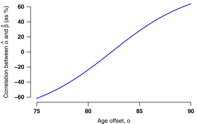
Figure A4 Correlation between
 $$\hat{\alpha }_{0} $$
and
$$\hat{\alpha }_{0} $$
and
 $$\hat{\beta }_{0} $$
for various values of offset age, o, in equation (A7). Data as in Table 2.
$$\hat{\beta }_{0} $$
for various values of offset age, o, in equation (A7). Data as in Table 2.
15.2. In practice, it would be necessary to determine o afresh for each portfolio (or for each altered age range for the same portfolio) if one wanted to eliminate the correlation between
 $$\hat{\alpha }_{0} $$
and
$$\hat{\alpha }_{0} $$
and
 $$\hat{\beta }_{0} $$
in equation (A7). This alone might argue for the simplicity of equation (10). However, the offset o also needs to be changed whenever the model changes. For example, we can introduce gender as a risk factor as in the following equation:
$$\hat{\beta }_{0} $$
in equation (A7). This alone might argue for the simplicity of equation (10). However, the offset o also needs to be changed whenever the model changes. For example, we can introduce gender as a risk factor as in the following equation:
 $$\mu _{{x_{i} }} \,{\equals}\,e^{{\alpha _{0} {\plus}\alpha _{{{\rm male}}} I_{{i,{\rm male}}} {\plus}\beta _{0} (x_{i} {\!\minus}\!o)}} $$
where I
i,male is an indicator variable taking the value 1 for males and 0 for females. Table A7 shows the correlations between the parameters, and the correlation between
 $$\hat{\alpha }_{0} $$
and
$$\hat{\alpha }_{0} $$
and
 $$\hat{\beta }_{0} $$
has strengthened due to the change in model. Furthermore, the correlation between
$$\hat{\beta }_{0} $$
has strengthened due to the change in model. Furthermore, the correlation between
 $$\hat{\alpha }_{0} $$
and
$$\hat{\alpha }_{0} $$
and
 $$\hat{\alpha }_{{{\rm male}}} $$
is large and cannot be easily eliminated. In fact, setting o=83 reduces the correlation between
$$\hat{\alpha }_{{{\rm male}}} $$
is large and cannot be easily eliminated. In fact, setting o=83 reduces the correlation between
 $$\hat{\alpha }_{0} $$
and
$$\hat{\alpha }_{0} $$
and
 $$\hat{\beta }_{0} $$
to −1%, but leaves the correlation between
$$\hat{\beta }_{0} $$
to −1%, but leaves the correlation between
 $$\hat{\alpha }_{0} $$
and
$$\hat{\alpha }_{0} $$
and
 $$\hat{\alpha }_{{{\rm male}}} $$
almost unchanged at −64%. Thus, our mis-estimation methodology must take account of parameter correlations as they cannot be avoided. We therefore prefer to use the simpler model structure of equation (10) without the orthogonalising constant in equation (A7).
$$\hat{\alpha }_{{{\rm male}}} $$
almost unchanged at −64%. Thus, our mis-estimation methodology must take account of parameter correlations as they cannot be avoided. We therefore prefer to use the simpler model structure of equation (10) without the orthogonalising constant in equation (A7).