I. INTRODUCTION
The problems connected with high-frequency mounting the function of the multiconductor transmission lines (MTLs) are various (crosstalk, distortion, attenuation, etc.). Skin and proximity effects make the problem more complicated, because the inclusion of these effects requires a model of distributed line with linear parameters related to frequency. They are, then, aggravated as a result of the propagation effects whenever the length of the interconnection liaison becomes large in relation to the wavelength. The traditional models of such liaisons (localized constant model or the cascade model) have become old-fashioned.
The major difficulty is then to have a distributed MTL model with losses (resistive, dielectric) valid in both time and frequency domains for linear and non-linear charges.
Diverse publications [Reference Paul1] have addressed this problem by using a modeling of cell cascade. This method provokes not only the oscillations of the echelon response (Heaviside function; Gibbs phenomenon [Reference Bakoglu2]), but also it needs an extreme important calculus time that penalizes simulation greatly. Furthermore, it is very difficult to model MTL with linear parameters based on the frequency. The modal method [Reference Paul1] that allows to represent MTLs, with the help of the BRANIN model [Reference Branin3–Reference Mejdoub, Saih, Rouijaa and Ghammaz5], is easy to be implemented in circuit simulators, but it does not permits to be tackled as lines without losses.
In this paper, we will focus basically on the general characteristics of the method developed by Dounavis et al. [Reference Dounavis, Xin, Nakhla and Achar6] to model MTL variable losses. This method, which is based on Padé approximation [Reference Baker and Graves-Morris7, Reference Rouijaa8] allows one to represent an MTL under, the “macro-model” form. Contrary to traditional cell method, this method does not present the Gibbs phenomenon; it can be easily integrated in generic or circuit simulators of type SPICE or ESACAP [Reference Stangerup9] using the MNA method “Modified Nodal Analysis” [Reference Ho, Ruehli and Brennan10].
Our contribution resides in macro-model optimization size, and therefore the reduction of variables number (macro-model matrix size) and subsequently the reduction of simulation duration. We show the specificities of the macro-model that we have developed and illustrate the importance of this model through various application examples.
II. PADE MARCO-MODEL: FROM LINE TO EQUIVALENT CIRCUIT
A) Reminder: MTL general equations
We consider MTL represented by Laplace parameter s through a coupled equation as below [Reference Paul11]:
 $$\left\{\matrix{\displaystyle{{\delta} \over {\delta z}}V\lpar z\comma \; s\rpar =- \lpar R+sL\rpar I\lpar z\comma \; s\rpar \comma \; \hfill \cr \displaystyle{\delta \over {\delta z}}I\lpar z\comma \; s\rpar =- \lpar G+sC\rpar V\lpar z\comma \; s\rpar \comma \; \hfill} \right.$$
or R, L, C and G ∈ ℜ N × ℜ N are matrix of linear parameters, and z is the propagation axis.
The solution of system (1) takes the form:
 $$\left[\matrix{V\left({\ell\comma \; s} \right)\hfill \cr - I\lpar \ell\comma \; s\rpar \hfill} \right]=e^Z \left[\matrix{V\left({0\comma \; s} \right)\hfill \cr I\lpar 0\comma \; s\rpar \hfill} \right]\comma \;$$
with
 $Z=\left[{\matrix{ 0 & { - \left({R+sL} \right)\ell } \cr { - \left({G+sC} \right)\ell } & 0 \cr } } \right]$
ℓ is the line length.
$Z=\left[{\matrix{ 0 & { - \left({R+sL} \right)\ell } \cr { - \left({G+sC} \right)\ell } & 0 \cr } } \right]$
ℓ is the line length.
The method proposed in [Reference Dounavis, Xin, Nakhla and Achar6] permits approximating the solution of equation (2) in the time domain.
B) Pade method: application to MTL
1) MATHEMATIC FORMULATION
Pade developments used in the field of enslaved systems to approximate a pure delay by a quotient of two polynomials have recently been applied in the analysis of the MTL. In this case, we extrapolate the previous method using the developments of Pade [Reference Baker and Graves-Morris7, Reference Rouijaa8] for the approximation of the exponential function matrix
 $e^Z $
. Thus, equation (2) becomes:
$e^Z $
. Thus, equation (2) becomes:
 $$\left[\matrix{V\left({\ell\comma \; s} \right)\hfill \cr - I\lpar \ell\comma \; s\rpar \hfill} \right]=e^Z \left[\matrix{V\left({0\comma \; s} \right)\hfill \cr I\lpar 0\comma \; s\rpar \hfill} \right]=B_{pq} \left(Z \right)^{ - 1} A_{pq} \left(Z \right)\left[\matrix{V\left({0\comma \; s} \right)\hfill \cr I\lpar 0\comma \; s\rpar \hfill} \right]\comma \;$$
with
 $$A_{pq} \lpar Z\rpar =\sum\limits_{j\;=\;1}^p {\displaystyle{{\lpar p+q+j\rpar !p!} \over {\lpar p+q\rpar !j!\lpar p - j\rpar !}}\lpar Z\rpar ^j }\comma \;$$
 $$B_{pq} \lpar Z\rpar =\sum\limits_{j\;=\;1}^q {\displaystyle{{\lpar p+q+j\rpar !q!} \over {\lpar p+q\rpar !j!\lpar q - j\rpar !}}\lpar Z\rpar ^j }\comma \;$$
or p and q represent the Pade approximation order, B pq −1(Z) and A pq (Z) are polynomials of matrices.
Using diagonal Pade approximation ( p = q ), we can express polynomials product B pq −1(Z).A pq (Z) using poles and zeros [Reference Rouijaa8]:
-
• p = 2.k pair:
(6) $$\eqalignno{B_{pq} \lpar Z\rpar ^{ - 1} A_{pq} \lpar Z\rpar & =\mathop \prod \limits_i^{\theta\;=\;p/2} \underbrace {\left[{\lpar u_i {\bi I} - Z\rpar \lpar u_{_i }^\ast {\bi I} - Z\rpar } \right]^{ - 1} }_{B_{pqi}^{-1} } \cr &\quad\, \underbrace {\left[{\lpar u_i {\bi I}+Z\rpar \lpar u_{_i }^\ast {\bi I}+Z\rpar } \right]^{ - 1} }_{A_{pqi}}.}$$
I is the identified matrix N × N.
with u i = x i + jy i , Polynomial complex pole B pq (Z), u i * is the conjugated pole.
-
• p = 2.k + 1 impair:
(7)
$$\eqalign{& B_{pq}^{ - 1} \lpar Z\rpar \, A_{pq} \lpar Z\rpar =\underbrace {\left({u_0 {\bi I} - Z} \right)^{ - 1} }_{B_{pq0}} \underbrace {\left({u_0 {\bi I}+Z} \right)}_{A_{pq0} } \cr & \quad \times \prod\limits_{i=1}^k {\underbrace {\left[{\left({u_i - Z} \right)\left({u_i ^\ast {\bi I} - Z} \right)} \right]^{ - 1} }_{B_{pqi}^{ - 1} }} \underbrace {\left[{\left({u_i {\bi I}+Z} \right)\left({u{_i }^\ast {\bi I}+Z} \right)} \right]}_{A_{pqi} }}$$
with u 0, polynomial real pole B pq (Z).


2) PADE MACRO-MODEL
From the previous equations, it is possible to determine an equivalent macro-model. Let us consider, for instance, the case of p impair. From equations (3) and (7), the transmission line can, then, be modeled by a macro-model that is constituted from a plurality cells of the first and the second order (cells with real and complex poles) whose number depends on the Pade approximation order (Fig. 1).
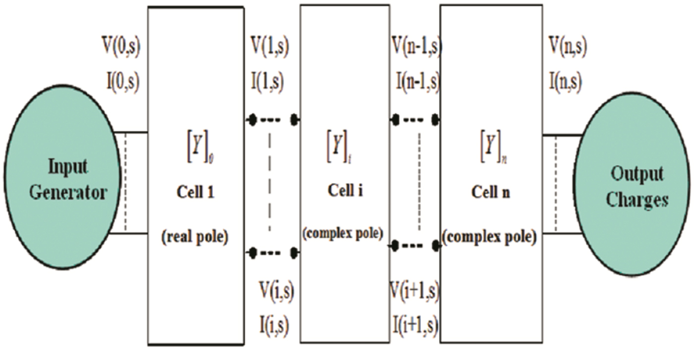
Fig. 1. Line equivalent circuit according to Pade: the first- and second-order cells.
We can relate the tension, input, and output current vectors of each cell of the Fig. 1 to its hybrid matrix.
-
1) Cell of real pole
Cell of real pole is defined by the hybrid representation
 $$\left[\matrix{V_\ell \hfill \cr I_\ell \hfill} \right]=B_{pq_0 }^{ - 1} \lpar Z\rpar A_{pq_0 } \lpar Z\rpar \left[\matrix{V_0 \hfill \cr I_0 \hfill} \right]\comma \;$$
 $${\rm with} \;B_{pq_0 }=\lpar u_0 {\bi I} - Z\rpar \comma \;$$
 $$A_{pq_0 }=\lpar u_0 {\bi I}+Z\rpar \comma \;$$
or
-
– V ℓ, I ℓ, V 0 and I 0 are, respectively, input and output variables
-
– I is the matrix unity.
-
2) Cell of complex pole
The cell of complex pole is defined by the hybrid representation
 $$\left[\matrix{V_{i+1} \hfill \cr I_{i+1} \hfill} \right]=B_{pqi}^{ - 1} \lpar Z\rpar A_{pq_i } \lpar Z\rpar \left[\matrix{V_i \hfill \cr I_i \hfill} \right]\comma \; \quad i=1\comma \; \ldots\comma \; n - 1$$
with
 $$A_{pqi}=\lpar u_i {\bi I}+Z\rpar \lpar u_i ^\ast {\bi I}+Z\rpar \comma \;$$
 $$B_{pqi}=\lpar u_i {\bi I}+Z\rpar \lpar u_i ^\ast {\bi I} - Z\rpar .$$
The vectors V 1, …, V n−1 and I 1, …, I n−1 are the intermediary variables that can be used for representing the macro-model.
3) DETERMINATION OF PADE APPROXIMATION ORDER
Pade approximant order ( p , q ) is determined with the help of the following inequality:
 $$\displaystyle{{\left\Vert {e^{\lsqb Z \rsqb } - B_{pq}^{ - 1} \lpar Z\rpar A_{pq} \lpar Z\rpar } \right\Vert } \over {\left\Vert {e^{\lsqb Z \rsqb } } \right\Vert _\infty }}\lt \xi _r$$
with ξ r the relative value of the error on the matrix exponential.
In the numeric approach, we have used the recurrence relations as follows:
 $$\displaystyle{{\left\Vert {B_{p+1q+1}^{ - 1} \lpar Z\rpar A_{p+1q+1} \lpar Z\rpar - B_{pq}^{ - 1} \lpar Z\rpar A_{pq} \lpar Z\rpar } \right\Vert _\infty } \over {\left\Vert {B_{p+1q+1}^{ - 1} \lpar Z\rpar A_{p+1q+1} \lpar Z\rpar } \right\Vert _\infty }}\lt \xi _r$$
with
 $$\fleqalignno{B_{pq} \lpar Z\rpar & =B_{p - 1q} \lpar Z\rpar +Z\left({\displaystyle{{ - q} \over {\lpar q+p\rpar \lpar q+p - 1\rpar }}} \right)B_{p - 1q - 1} \lpar Z\rpar \matrix{\comma \; \cr } \cr & \quad p \geq l\comma \; q \geq l\comma \;}$$
 $$B_{pq} \lpar Z\rpar =B_{pq - 1} \lpar Z\rpar +Z\left({\displaystyle{p \over {\lpar q+p\rpar \lpar q+p - 1\rpar }}} \right)B_{p - 1q - 1} \lpar Z\rpar \comma \;$$
 $$A_{pq} \lpar Z\rpar =B_{p - 1q} \lpar Z\rpar +Z\left({\displaystyle{p \over {\lpar q+p\rpar \lpar q+p - 1\rpar }}} \right)A_{p - 1q - 1} \lpar Z\rpar \comma \;$$
 $$B_{pq} \lpar Z\rpar =B_{pq - 1} \lpar Z\rpar +Z\left({\displaystyle{{ - q} \over {\lpar q+p\rpar \lpar q+p - 1\rpar }}} \right)B_{p - 1q - 1} \lpar Z\rpar .$$
In a simulation, the value ξ r relates to the used application (time or frequency domain) and to precision constraints in these domains.
III. MODEL STABILITY AND PASSIVITY
The study of a complete circuit comprises generally a source of excitement, a transmission line, and output load. The study of such circuit imposes typically a problem of model stability. The problem of the equivalent circuit stability can be approached in many ways. We are interested, as in the case of the extern stability, in the evolution of circuit output excited by a certain stimulus (stability BIBO, i.e. bounded input–bounded output). We study, in the case of the intern stability, the natural evolution of circuit analyzing the transient evolution of an adapted scalar function, such as the total energy and its derivative (Lyapunov stability). In a hybrid approach, we can analyze the energetic evolution of circuit excited by any input entry. This approach, since it corresponds the notion of passivity [Reference Lozano, Brogliato, Egeland and Maschke12], is considered as the most suitable for our case.
The analysis of the different constraints related to the stability, causality, and passivity, was conducted in [Reference Triverio, Grivet-Taloua, Nakhla, Canaveo and Achar13]. Comparison of the stresses associated with these concepts show that passivity presents the most interesting proprieties but also the hardest constraints.
Thus, the association of two macro-models, stable individually, does not guarantee the stability of the whole [Reference Feldmann14, Reference Desoer and Kuh15]. As against the property of passivity is essential as it ensures the stability of all macro-models constituting the circuit: if a model is passive, it is necessarily stable (the reverse is not always true) and the association of two passive models, resulting in an overall passive model. Given these properties, it will suffice that the Pade macro-model is passive to ensure a complete passivity of the entire network (the other network elements are assumed to be passive) and, subsequently, its stability [Reference Rouijaa8].
Recalling that, from a physical point of view, the passivity or “dissipativity” means that the energy of the system at time T is less than or equal to the sum of the initial energy and the energy supplied to the circuit during the interval (0, T) by the external source. It corresponds to the following mathematical definition:
 $$W\lpar T\rpar \leq W\lpar 0\rpar +\vint_0^T {V\lpar \tau \rpar .I\lpar \tau \rpar .d\tau } .$$
Applied to the n-port networks study, it leads to the following two conditions [Reference Dounavis, Achar and Nakhla16] that must satisfy the admittance matrix Y (s):
-
• Y (s*) = Y *(s)
-
• Y (s): the real positive definite matrix
The first condition implies that the coefficients of the rational matrix are real: this condition is always verified.
It will suffice, then, to ensure that Y (s) is a real positive matrix for all Re(s) > 0 to guarantee the model stability.
As we mentioned earlier, Pade macro-model is composed of cells and complex real poles. According to the criterion of passivity, it is sufficient that these two cells are passive (Y 0 and Y i are real positives) for the macro-model is passive and therefore stable.
Admittance matrices Y 0 and Y i contain linear parameters of the line R, L, C, and G. All these matrices are real positive and then the Pade macro-model is passive [Reference Dounavis, Xin, Nakhla and Achar6].
IV. MNA METHOD: FROM EQUIVALENT CIRCUIT TO APPLIED EQUATIONS
A) MNA method
The “Modified Nodal Approach” MNA method [Reference Rouijaa8, Reference Ho, Ruehli and Brennan10] is a method based on Kirchhoff laws, which is applied to every type circuit constituted from passive elements (linear and/or non-linear) and active ones (independent excitement sources). This mixed method permits to use the tensions and currents like unknown variables in a circuit simultaneously.
The relations (8) and (11) can be represented as follows:
 $$G_\pi \left[\matrix{V \hfill \cr I \hfill} \right]+C_\pi \left[\matrix{V \hfill \cr I \hfill} \right]=\left[\matrix{J \hfill \cr F \hfill} \right].$$
The matrices C π and G π contain the passive elements (R, L, C, and G).
MNA method is easy to be implemented especially if we know the network description and output requirement. The calculus leads to sparse matrices, which are well adapted to digital computation.
B) MNA method application of Pade macro-model
Using the circuits theory [Reference Kuh and Rohrer17, Reference Louis18] and from the admittance matrix of each cell (Y 0 and Y i ), we obtain two equivalent electric schema related to each cell (real and complex cell poles). MNA method application of electric schema, corresponding to each cell, leads to these matrices C π and G π. The size of the matrices C π and G π has been reduced (see Table 1) to the proposed [Reference Dounavis, Achar and Nakhla19] work. Optimized expressions of these matrices are given below.
Table 1. Optimization of matrices C π and G π.

The determination of state equation (MNA method) from electric schema and blocks optimization will be given with more detail in the following paragraph.
1) CELL OF REAL POLE
From the admittance matrix of the cell real pole, we get the equivalent electric schema below (Fig. 2).
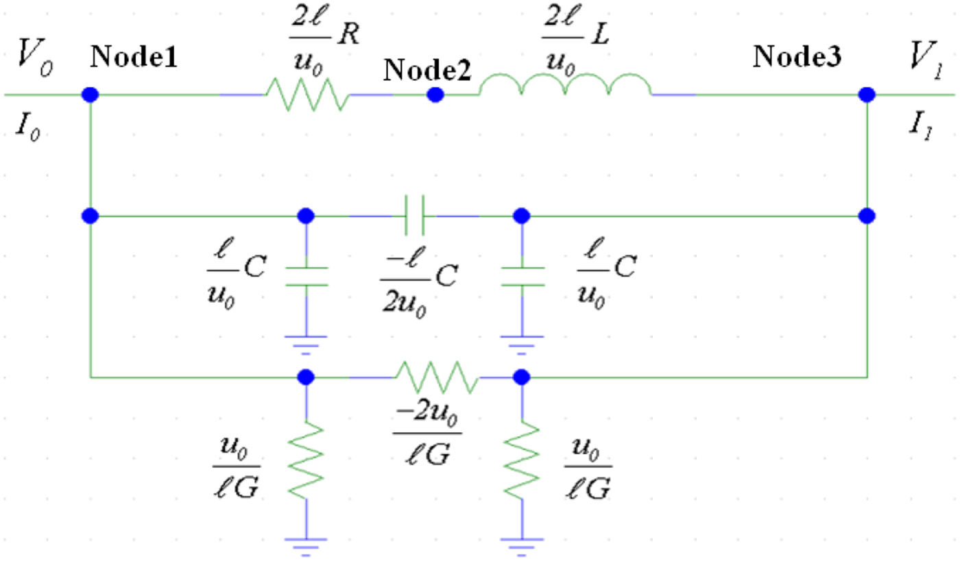
Fig. 2. Equivalent schema of cell real pole.
The representation of this circuit is difficult to be generalized in the case of MTL. Of course, this method is not systematic at all: it is necessary to redefine the equivalent schema of each studied case. In addition, the number of quadruple and the number of elements (RLC) in question become very important. Finally, the equivalent circuit is further complicated by the addition of the coupling impedances.
MNA method application of schema (cell of real pole), leads to the matrices
 $C_\pi $
and
$C_\pi $
and
 $G_\pi $
their expressions are given below:
$G_\pi $
their expressions are given below:
Matrice G π, Matrice C π
 $$\eqalign{& G_\pi=\mathop {\left[{\matrix{ {node1} & {node2} & {node3} & I_L \cr {\displaystyle{\ell \over {2\mu _0 }}G} & 0 & {\displaystyle{\ell \over {2\mu _0 }}G} & I \cr 0 & {\displaystyle{{\mu _0 } \over {2\ell }}R^{ - 1} } & {\displaystyle{{ - \mu _0 } \over {2\ell }}R^{ - 1} } & { - I} \cr {\displaystyle{\ell \over {2\mu _0 }}G} & {\displaystyle{{ - \mu _0 } \over {2\ell }}R^{ - 1} } & {\left({\displaystyle{{\mu _0 } \over {2\ell }}R^{ - 1}+\displaystyle{\ell \over {2\mu _0 }}G} \right)} & 0 \cr { - I} & I & 0 & 0 \cr } } \right]}\comma \; \cr & \quad C_\pi=\mathop {\left[{\matrix{ {node1} & node2 & {node3} & {I_L } \cr {\displaystyle{\ell \over {2\mu _0 }}C} & 0 & {\displaystyle{\ell \over {2\mu _0 }}C} & 0 \cr 0 & 0 & 0 & 0 \cr {\displaystyle{\ell \over {2\mu _0 }}C} & 0 & {\displaystyle{\ell \over {2\mu _0 }}C} & 0 \cr 0 & 0 & 0 & {\displaystyle{{2\ell } \over {\mu _0 }}L} \cr } } \right]} .}$$
It is possible to simplify the matrices
 $C_\pi $
and
$C_\pi $
and
 $G_\pi $
taking into account the fact that the current in the resistance between nodes 1 and 2 is the same as the inductance between nodes 2 and 3. Also, it is possible to replace these two branches in one branch and reduce the dimensions of matrices according to the following expressions (node 2 is deleted).
$G_\pi $
taking into account the fact that the current in the resistance between nodes 1 and 2 is the same as the inductance between nodes 2 and 3. Also, it is possible to replace these two branches in one branch and reduce the dimensions of matrices according to the following expressions (node 2 is deleted).
Matrice G π, Matrice C π :
 $$\eqalign{& G_\pi=\mathop {\left[{\matrix{ {node1} & {node2} & {I_{L1}} \cr {\displaystyle{\ell \over {2\mu _0 }}G} & {\displaystyle{\ell \over {2\mu _0 }}G} & I \cr {\displaystyle{\ell \over {2\mu _0 }}G} & {\left({\displaystyle{{\mu _0 } \over {2\ell }}R^{ - 1}+\displaystyle{\ell \over {2\mu _0 }}G} \right)} & { - I} \cr { - I} & I & {\displaystyle{{2\ell } \over {\mu _0 }}R} \cr } } \right]}\cr \comma \; \cr & \quad C_\pi=\mathop {\left[{\matrix{ {node1} & {node2} & {I_{L1}} \cr{\displaystyle{\ell \over {2\mu _0 }}C} & {\displaystyle{\ell \over {2\mu _0 }}C} & 0 \cr {\displaystyle{\ell \over {2\mu _0 }}C} & {\displaystyle{\ell \over {2\mu _0 }}C} & 0 \cr 0 & 0 & {\displaystyle{{2\ell } \over {\mu _0 }}L} \cr } } \right]}.}$$
2) CELL OF COMPLEX POLE
As we have seen before, it is possible to determine the matrices
 $C_\pi $
and
$C_\pi $
and
 $G_\pi $
of the cell complex pole.
$G_\pi $
of the cell complex pole.
Matrice G π:
 $$\eqalign{&G_\pi=\left[{\matrix{ {\displaystyle{{x_i^2+y_i^2 } \over {4x_i \ell }}R^{ - 1}+\displaystyle{\ell \over {4x_i }}G} & 0 & {\displaystyle{\ell \over {4x_i }}G} \cr 0 & {\displaystyle{{x_i \ell } \over {x_i^2+y_i^2 }}G} & {\displaystyle{{ - x_i \ell } \over {x_i^2+y_i^2 }}G}\cr {\displaystyle{\ell \over {4x_i }}G} & {\displaystyle{{ - x_i \ell } \over {x_i^2+y_i^2 }}G} & {\left({\displaystyle{{x_i \ell } \over {x_i^2+y_i^2 }}+\displaystyle{\ell \over {4x_i }}} \right)G}\cr {\displaystyle{{x_i^2+y_i^2 } \over {4x_i \ell }}R^{ - 1} } & 0 & 0 \cr { - I} & I & 0 \cr 0 & 0 & { - I} \cr } } \right.\cr &\qquad \qquad \qquad \qquad \qquad \left.{\matrix{ {\displaystyle{{x_i^2+y_i^2 } \over {4x_i \ell }}R^{ - 1} } & I & 0 \cr 0 & { - I} & 0 \cr 0 & 0 & I \cr {\displaystyle{{x_i^2+y_i^2 } \over {4x_i \ell }}R^{ - 1} } & 0 & { - I} \cr 0 & {\displaystyle{\ell \over {x_i }}R} & 0 \cr I & 0 & 0 \cr } } \right].}$$
Matrice C π:
 $$C_\pi=\left[{\matrix{ {\displaystyle{\ell \over {4x_i }}C} & 0 & {\displaystyle{\ell \over {4x_i }}C} & 0 & 0 & 0 \cr 0 & {\displaystyle{{x_i \ell } \over {x_i^2+y_i^2 }}C} & {\displaystyle{{ - x_i \ell } \over {x_i^2+y_i^2 }}C} & 0 & 0 & 0 \cr {\displaystyle{\ell \over {4x_i }}C} & {\displaystyle{{ - x_i \ell } \over {x_i^2+y_i^2 }}C} & {\left({\displaystyle{{x_i \ell } \over {x_i^2+y_i^2 }}+\displaystyle{\ell \over {4x_i }}} \right)C} & 0 & 0 & 0 \cr 0 & 0 & 0 & 0 & 0 & 0 \cr 0 & 0 & 0 & 0 & {\displaystyle{\ell \over {x_i }}L} & 0 \cr 0 & 0 & 0 & 0 & 0 & {\displaystyle{{4x_i \ell } \over {x_i^2+y_i^2 }}L} \cr } } \right].$$
Knowing the matrices C π and G π, we have implemented the state equation defined by MNA method in circuit simulator ESACAP [Reference Stangerup9]. In the following paragraph, we present an example of simulations realized depending on our circuit approach.
V. APPLICATION: TRANSIENT ANALYSIS OF THREE MICROSTRIP LINES PCB WITH A PERFECTLY CONDUCTING GROUND PLANE
In this example, an extract is taken from the study done by Chang in 1970 [Reference Chang20]. We will compare the induced tensions in transient analysis in two receptor conductors (near- and far-crosstalk tensions) obtained through Pade Macro-model with the decomposition method in cells cascade. Let us consider three rectangular conductors placed in a non-homogeneous dielectric (ε r = 4.65) with electrical reference for conducting ground plane perfectly. These conductors are excited by a generator e(t) internal impedance 50 Ω, rise time T r = 1 ns, delivering an echelon of 1 V amplitude (Fig. 3).

Fig. 3. Three-wire line electric schema.
Depending on these geometric parameters of the three ribbons defined in Fig. 4, the linear parameters R, L, and C are presented below [Reference Gilles21, Reference Inzoli and Rouijaa22]:
 $$\eqalign{L & =\left[{\matrix{ {3.879} & {1.6238} & {0.8252} \cr {1.6238} & {3.7129} & {1.6238} \cr {0.8252} & {1.6238} & {3.879}} } \right]\, {\rm nH/cm\comma \; } \cr \quad C &=\left[{\matrix{ {1.0413} & { - 0.3432} & { - 0.014} \cr { - 0.3432} & {1.1987} & { - 0.3432} \cr { - 0.014} & { - 0.3432} & {1.0413}} } \right]\, {\rm pF/cm\comma \; }}$$
 $$\eqalign{R & =\left[{\matrix{ {R_{dc} } & 0 & 0 \cr 0 & {R_{dc} } & 0 \cr 0 & 0 & {R_{dc} }} } \right]\, \Omega /{\rm cm\comma \; } \cr \quad R_{dc} & =\displaystyle{1 \over {\sigma wd}}=3.18\, \Omega /{\rm cm}\; ^{\hbox{\lpar see\ e.g.\comma Paul \lsqb 1\rsqb \rpar }}}$$
with σ = 58 m/mm2, copper conductivity.

Fig. 4. Sectional view of three rectangular conductors immersed in a dielectric.
The comparison with a rigorous analytical approach is difficult to be realized because the dielectric is non-homogenous. The frequency range is very high; the conductors' number is important and all these present further losses.
It is possible to determine an equivalent homogenous dielectric medium introducing a constant and effective dielectric, such as
 $\varepsilon _e \colon \varepsilon _e=\displaystyle{{1+\varepsilon _r } \over 2}.$
Also, the propagation time is:
 $\Delta T=\displaystyle{l \over \nu }=1.7\, {\rm ns}\matrix{\semicolon \; \cr } \; \nu=\displaystyle{{3.10^8 } \over {\varepsilon _e }}$
(see, e.g., [Reference Paul1]).
$\Delta T=\displaystyle{l \over \nu }=1.7\, {\rm ns}\matrix{\semicolon \; \cr } \; \nu=\displaystyle{{3.10^8 } \over {\varepsilon _e }}$
(see, e.g., [Reference Paul1]).
Figures 5 and 6 show the evolution of the far- and near-crosstalk tensions in terms of time in the case of cell model and Pade macro-model. The first method uses 766 variables, whereas the macro-model uses only 65 variables (see Table 2).

Fig. 5. Transient response of the input tensions of the three conductors (far-crosstalk).
Fig. 6. Transient response of the output tensions of the three conductors (near-crosstalk).
Table 2. Comparison between cells decomposition method and Pade macro-model.
The different curves clearly show the return time (3.4 ns or 2xΔT; ΔT = 1.7 ns delay line) associated with different mismatches in and out of the line.
We note that T = 1.5 ns (Fig. 5), the tension V 1a of the generator conductor input equals the value 0.55 V: this value corresponds the potentiometric division to input impedance of disruptive conductor, Z in1 = 68 Ω which also represents, due to the absence of the effects of propagation up to this time, the characteristic impedance of the line.
The disruptive conductor mismatch is from the origin of the augmentation of the tension V 1a from the moment T = 3.4 ns (positive reflection).
Far- and near-crosstalk tensions have substantially the same shape.
The very small rise time of the generator (T r = 1 ns, equivalent bandwidth of the order of 350 MHz) does not obviously allow to represent by localized elements, and consequently a simple physical interpretation of crosstalk phenomenon. The analytical method [Reference Vabre23] used for the study of weak coupling in the three-wire lines could possibly be extrapolated to interpret qualitatively the curves.
Finally, the simulation results are in good concordance with those from the measurements [Reference Chang20].
Table 2 below sums up the main interest of our method in terms of its relation to the method of decomposition cells.
VI. CONCLUSION
In this paper, we have presented a new digital model of transmission lines using a circuit approach. This method is based on the transmission lines theory, which is also based on the Pade approximation of exponential matrix. Its software implementation has been carried out by the MNA method.
First, we determined the admittance matrix of the line based on linear parameters thereof and Pade polynomials. This admittance matrix was associated with a model called Pade macro-model. Also, we analyzed its problems of stability and passivity.
Finally, the macro-model also allows one to take into account the losses in the lines. In the presented application examples, we compared the performance of our model with the cells cascade model. Through these examples, we have shown the optimization interests of Pade model compared to cells method: the reduction of variables number and blocks leads consequently to a reduction of simulation duration.
The extension of the macro-model LTM with varying losses with frequency is an interesting possibility to model real situations. In the same process, it will be interesting to extend the case of LTM excited by EM wave and LTM shielded.
 Youssef Mejdoub was born in Morocco, in 1980. He received the DESA (6 years study after the baccalaureate, equivalent to Master) in Telecommunications & Network from Cadi Ayyad University, Marrakech Morocco, in 2007. He is a Ph.D. student in Electrical Systems and Telecommunications Laboratory LSET at Cadi Ayyad University – Marrakech – Morocco. His research interest includes the electromagnetic compatibility, multiconductor transmission lines, and telecommunications.
 Hicham Rouijaa is a Professor of Physics, attached to Cadi Ayyad University, Marrakech Morocco. He obtained his Ph.D. thesis on Modeling of Multiconductor Transmission Lines, in 2004, from Aix-Marseille University – France. He is an associate member of Electrical Systems and Telecommunications Laboratory LSET at the Cadi Ayyad University. His current research interests concern electromagnetic compatibility and multiconductor transmission lines.
 Abdelilah Ghammaz received the Ph.D. degree of Electronic from the National Polytechnic Institut (ENSEEIHT) of Toulouse, France, in 1993. In 1994, he went back to Cadi Ayyad University of Marrakech – Morroco. Since 2003, he has been a Professor at the Faculty of Sciences and Technology, Marrakech, Morroco. He is a member of Electrical Systems and Telecommunications Laboratory LSET at the Cadi Ayyad University. His research interests concern electromagnetic compatibility, multiconductor transmission lines, telecommunications, and antennas.