2. Formulation of the basic equations: quasi-gesostrophic limit

Consider motions in a rotating system in which the standard scaling applies; that is, the horizontal coordinates are scaled by L, the horizontal velocities by U and the time by L/U. The vertical velocity is scaled by UD/L and the pressure anomaly by $\rho _{o}2\varOmega UL$ , where $\varOmega$ is the magnitude of the rotation whose axis is now inclined at an angle $\theta$ with respect to the y axis (which, as usual, points northward). The dimensional density is written as $\rho _{*}=\rho _{o}(1+2(({\varOmega UL})/({gD}))\rho )$ , where $\rho _{*}$ is the dimensional density and $\rho _{o }$ is the basic state density which may also be a function of z, the vertical coordinate. As is standard, the perturbation density and pressures are small compared with their resting values $p_{o}$ and $\rho _{o }$ .

The non-dimensional equations of motion are then the momentum equations, which ignoring friction are

(2.1a) \begin{align} \epsilon \frac{{\rm d}u}{{\rm d}t}-\sin\theta v+\delta \cos\theta w&=-\frac{\partial p}{\partial x}, \end{align}

(2.1b) \begin{align} \epsilon \frac{{\rm d}v}{{\rm d}t}+\sin\theta u&=-\frac{\partial p}{\partial y},\end{align}

(2.1c) \begin{align} \epsilon \delta ^{2}\frac{{\rm d}w}{{\rm d}t}-\delta \cos\theta u&=-\frac{\partial p}{\partial z}-\rho.\end{align}

And the incompressibility condition which is valid because of the smallness of the Rossby number is

(2.1d) \begin{equation} \frac{\partial u}{\partial x}+\frac{\partial v}{\partial y}+\frac{\partial w}{\partial z}=0 .\end{equation}

The final equation is the energy equation which we simplify to conservation of density:

(2.1e) \begin{equation}\epsilon \frac{{\rm d}\rho }{{\rm d}t}-Sw=0.\end{equation}

The symbols are standard and $\epsilon$ is the Rossby number $U/2\varOmega L$ and is considered a small parameter. The stratification parameter, $S={(N^{2}D^{2})}/{(4\varOmega ^{2}L^{2})}$ , where N is the Brunt–Väisälä frequency, will be considered O(1)I as will the aspect ratio, $\delta .$ The aspect ratio now will be considered. The set (2.1) is immediately recognized as the form that the equations of motion take when written for motion on a sphere except that the metric terms in spherical coordinates have been replaced by their Cartesian equivalents, i.e. we are using a tangent plane model of the motion.

The operator d/dt is ${\partial }/({\partial t})+u({\partial }/{\partial x})+v({\partial }/{\partial y})$ , the vertical advection term being negligible from the conservation of density equation (2.1e ).

We proceed by an expansion in the Rossby number assuming that the aspect ratio, $\delta$ , is not small, at least in comparison with the Rossby number.

At the lowest order in $\epsilon$ , the above equations yield (assuming small w)

(2.2a,b,c) \begin{equation}\sin \theta u_{o}=-\frac{\partial p_{o}}{\partial y},\quad-\delta \cos \theta u_{o}=-\frac{\partial p_{o}}{\partial z}-\rho _{o},\quad\sin \theta v_{o}=\frac{\partial p_{o}}{\partial x}\end{equation}

The axis of rotation is tilted from the y axis by the angle $\theta$ so along that axis ${\partial z}/{\partial s}=\sin \theta$ and along the y axis ${\partial y}/{\partial s}=\cos \theta$ , combining (2.2a ) and (2.2b ):

(2.3) \begin{equation}\rho _{o}=-(1/\sin \theta )\partial p_{o}/\partial s.\end{equation}

It then follows from the lowest-order geostrophic balance that the familiar thermal wind equations for u _o and v_o become

(2.4a,b) \begin{equation}(\partial u_o)/\partial s=(\partial \rho_o)/\partial y,\quad(\partial v_o)/\partial s=-(\partial \rho_o)/\partial x.\end{equation}

Note that (2.4b ) holds even if $\delta \cos \theta w$ is retained in (2.2c ). The physical content of (2.4a,b ) involves the tilting of the planetary vorticity vector, which by definition is along the s axis, into the x and y directions by the velocity shear along that axis, i.e. by the change along the z axis and the horizontal axes as well. This result has also been found by de Verdiere & Schopp (Reference de Verdiere and Schopp2006).

Thus again, it is the axis of rotation that plays the role of the third axis of the problem. The spatial variation of the horizontal velocity occurs along the tilted rotation axis and not the vertical determined by gravity and, as a consequence, we will find ourselves dealing with the non-orthogonal $(x,y,s)$ coordinate system. In each case, the response to the lateral density gradient which would give rise to a forcing term for production of vorticity by the cross product of the pressure and density gradients is, instead, balanced by the tilting of the planetary vorticity. The tilting requires a shear in the horizontal velocity along the axis of the planetary vortex tube, e.g. the tilted axis of rotation.

At the next order in Rossby number, order $\epsilon$ , the momentum equations become

(2.5a) \begin{align} \frac{{\rm d}u_{o}}{{\rm d}t}-\sin \theta v_{1}+\delta \cos\theta w_{1}&=-\frac{\partial p_{1}}{\partial x}, \end{align}

(2.5b) \begin{align} \frac{{\rm d}v_{o}}{{\rm d}t}+\sin \theta u_{1}&=-\frac{\partial p_{1}}{\partial y}, \end{align}

(2.5c) \begin{align} -\delta \cos \theta u_{1}&=\frac{\partial p_{1}}{\partial z}-\rho _{1}, \end{align}

(2.5d) \begin{align} \frac{\partial u_{1}}{\partial x}+\frac{\partial v_{1}}{\partial y}+\frac{\partial w_{1}}{\partial z}&=0, \end{align}

(2.5e) \begin{align} \frac{{\rm d}\rho _{o}}{{\rm d}t}-Sw_{1}&=0,\end{align}

where the operator $\textrm{d}/{{\rm d}t}={\partial }/{\partial t}+u_{o}({\partial }/{\partial x})+v_{o}({\partial }/{\partial y})$ .

Cross-differentiating (2.5a,b) in the usual manner and using (2.5d ) we obtain the vorticity equation:

(2.6) \begin{equation}\frac{\partial \zeta _{o}}{\partial t}+u_{o}\frac{\partial \varsigma _{o}}{\partial x}+v_{o}\frac{\partial \varsigma _{o}}{\partial y}=\frac{\partial w_{1}}{\partial s}.\end{equation}

Thus, it is the stretching of the vertical component of the planetary vorticity along the vertical and the tilting of the horizontal component of the planetary vorticity into the vertical that are dynamically significant in changing the vorticity (see also (7.5) for another example of the physical content of this result). Using (2.3) and (2.5e ) in (2.6) yields the new quasi-geostrophic potential vorticity equation:

(2.7) \begin{equation}\frac{{\rm d}\varsigma _{o}}{{\rm d}t}+\frac{1}{\sin \theta }\frac{\rm d}{{\rm d}t}\left(\frac{\partial }{\partial s}\frac{1}{S}\frac{\partial p_{o}}{\partial s}\right)=0.\end{equation}

Again, we see that the variable that replaces the vertical coordinate z is the coordinate along the rotation axis. Also, from now on since $\delta$ is considered an O(1) parameter, I will just be set equal to 1 to make the algebra slightly neater.

The geostrophic streamfunction is $\psi =p_{o}/\sin \theta $ , in terms of which (2.7) becomes

(2.8) \begin{equation}\frac{\rm d}{{\rm d}t}\nabla ^{2}\psi +\frac{\rm d}{{\rm d}t}\left(\frac{\partial }{\partial s}\frac{1}{S}\frac{\partial \psi }{\partial s}\right)=0,\end{equation}

which will be our governing equation. This quasi-geostrophic equation in this form has appeared before in the literature.

It is important to note that the independent variables in (2.8) (x, y and s) are three variables that are not mutually orthogonal. Before proceeding further, we must discuss how to deal with this unusual situation.

Although it is clear from a physical point of view that s, the distance along the axis of the rotation vector, is the natural third coordinate, it is not clear whether y is the natural complementary coordinate. This is the focus of our discussion in § 3.

3. The coordinate system revisited

The results of the previous section suggest that the rotation axis, the direction upon which the motion changes, is a natural third coordinate, called s. What is the complementary coordinate? To find that direction consider the representation of an arbitrary point in the (y, z) or (y, s) plane in terms of the unit vectors j and s which, respectively, are aligned with the y axis and the s axis. Any vector V in the (y, z) or (y, s) plane can be written as a linear combination of two vectors in those directions. That is, for any V we can write

(3.1) \begin{equation}\boldsymbol{V}=A\boldsymbol{j}+B\boldsymbol{s}.\end{equation}

To find the coordinates of V in the (y, s) frame, i.e. A and B in this coordinate system, we can take the inner product of V with each of the unit vectors giving two equations for the coordinates A and B. The calculation is straightforward and the result is

(3.2a) \begin{align} A&=(\boldsymbol{V}\cdot \boldsymbol{j}-(\boldsymbol{V}\cdot \boldsymbol{s})(\boldsymbol{s}\cdot \boldsymbol{j}))/(1-(\boldsymbol{s}*\boldsymbol{j})^{\textbf{2}}), \end{align}

(3.2b) \begin{align} B&=(\boldsymbol{V}\cdot \boldsymbol{s}-(\boldsymbol{V}\cdot \boldsymbol{j})(\boldsymbol{s}\cdot \boldsymbol{j}))/(1-\left(\boldsymbol{s}*\boldsymbol{j})^{\textbf{2}}\right). \end{align}

Figure 1. A schematic showing the (y, z) plane and the s axis aligned with the rotation vector. An arbitrary point in the (y, z) plane has coordinates $z/\sin \theta$ on the s axis and its complementary coordinate $y_{o}$ on the y axis, as shown.

If V = y j + z k , i.e. the position vector, it follows that B, the coordinate along the s axis, i.e. s, is (note that $\textbf{s}\cdot \boldsymbol{j}=\cos \theta$ )

(3.3a) \begin{equation}B=\frac{z}{\sin \theta }=s\end{equation}

just what we would expect from a simple trigonometric argument. However, the natural coordinate along the y axis is more surprising. From the solution for A it follows that

(3.3b) \begin{equation}A=\left(y-z\frac{\cos \theta }{\sin \theta }\right)=(y-s \cos \theta ).\end{equation}

The result (3.3b ) may seem odd, but a little thought makes it more natural. First one can think about how we find those coordinates in the (y, z) system (see figure 1). From the point (y, z) we move horizontally, i.e. parallel to the y axis, until we intersect the z axis and that is the coordinate of the point on the z axis. We do the same to find the y coordinate, i.e. we move parallel to the z axis until we intersect the y axis to find the y coordinate. It is exactly the same in the tilted s system. From the point (y, z) in the plane we move parallel to the y axis until we strike the tilted s axis to find the s coordinate at $z/\sin \theta$ . Now we move parallel to the s axis until we strike the y axis, as shown in figure 1, and we find that intersection point at

(3.3c) \begin{equation}y_{0}=y-s\cos \theta,\end{equation}

and this is the result (3.3b ). In this system the natural coordinates are $x,\ s$ and $y_{0}$ .

Before proceeding further, we will examine a simple model problem that will, hopefully, make this more plausible.

First note that the partial derivative in y at constant z is the same as the derivative with respect to y _o at constant s. Consider the solution to the equation

(3.5) \begin{equation}\nabla ^{2}\psi +\frac{\partial }{\partial s}\frac{1}{S}\frac{\partial \psi }{\partial s}=0.\end{equation}

For the present purpose we consider the case where S is constant and then write the last term in (3.5) in x, y, z coordinates leading to

(3.6) \begin{equation}S\left(\frac{\partial ^{2}\psi }{\partial y^{2}}+\frac{\partial ^{2}\psi }{\partial x^{2}}\right)+(\sin \varTheta )^{2}\frac{\partial ^{2}\psi }{\partial z^{2}}+2\sin \varTheta \cos \varTheta \frac{\partial ^{2}\psi }{\partial y\partial z}+\left(\cos \theta \right)^{2}\frac{\partial ^{2}\psi }{\partial y^{2}}=0.\end{equation}

We can find a solution of the form $\psi =\phi (z){\rm e}^{ily+ikx}$ . The equation for $\phi (z)$ is simply

(3.7) \begin{equation}\phi _{ZZ}+2il \phi _{z}\frac{\cos \theta }{\sin \theta }\sin \theta -\phi \left(\frac{S\left(k^{2}+l^{2}\right)}{(\sin \theta )^{2}}\right)+l^{2}\left(\frac{\cos \left(\theta \right)}{\sin \left(\theta \right)}\right)^{2}=0,\end{equation}

the solution of which leads to

(3.8) \begin{equation}\psi ={\rm e}^{il(y - s\cos \theta )+ikx}\big(A{\rm e}^{-Ks}+B{\rm e}^{Ks}\big),\quad K^{2}=S\big(k^{2}+l^{2}\big),\end{equation}

where we have used $s=z/\sin \theta$ . Note that the first exponential in (3.8) is simply our new friend, $y_{o}$ . This is an illustration of how the natural coordinates of our problem are the variables s and $y_{o}$ rather than y and z. We shall profit from this example in the next section when we take up the Eady problem with the tilted rotation vector.

4. The Eady problem

The model, first proposed by Eady (Reference Eady1949), considers a flow produced by a constant meridional density gradient in the y direction and the thermal wind thus produced the basic state whose stability is examined. In Eady’s problem, that gives rise to a flow in the x direction increasing linearly with height, e.g. z. As we have shown, in our model with the tilted rotation vector, linear variation occurs with s, the coordinate along the axis of rotation. Thus, our streamfunction consists of the basic state, a zonal velocity in

(4.1) \begin{equation}U_{o}=\lambda s.\end{equation}

We write the perturbation streamfunction as

(4.2) \begin{equation}\phi =A{\rm e}^{ikx+il{y_{o}}-ikct} F(s),\end{equation}

where the real part is understood, while, as in the example of § 3, $F$ satisfies

\begin{equation*} F_{ss}-S(k^{2}+l^{2})F=0, \end{equation*}

the solution of which as before can be written

(4.3) \begin{equation}F\left(s\right)=A\sinh \left(Ks\right)+\textit{B}\,\textrm{cosh}(Ks),\end{equation}

where $K^{2}=S(k^{2}+l^{2})$ . The boundary conditions on z = 0 and $z=D=s \sin \theta$ imply that D in the classical stability criterion is replaced by ${D}/{\sin\theta }$ and thus the condition becomes, for $\delta =1$ ,

(4.4) \begin{equation}K\lt 2.3994\sin \theta.\end{equation}

Thus, as the tilt gets larger, i.e. the rotation axis approaches the horizontal and $\sin \theta$ goes to zero, the instability becomes expunged since K has a minimum given by l. The tilt thus stabilizes the flow. The fundamental reason for this change is that, as in the original formulation, the Eady model becomes stabilized if the two boundaries are far enough apart so that they no longer interact, given the exponential decay of the perturbations from the horizontal boundaries. In the tilted case, the distance between the boundaries is measured in s and as the tilt becomes larger the distance in s increases like $1/\sin \theta$ .

5. The beta effect

As was remarked upon in § 2, the governing equations given there have the same form as the equations of motion written on a sphere with $\theta$ as the latitude. The Cartesian coordinates used can be interpreted as the coordinates on the tangent plane to the sphere at that latitude. In just the same way as is usually done, we can include the spatial variations of those trigonometric terms by including small variations in the north–south distance y from the central latitude. Thus if L is a characteristic spatial departure from the central latitude and if R is the sphere’s radius and if $L/R$ is $O(\epsilon )$ , expanding the trigonometric functions gives us the beta plane extension of the horizontal momentum equations, from which the vorticity equation directly follows:

(5.1) \begin{equation}\frac{{\rm d}\varsigma _{o}}{{\rm d}t}+\frac{1}{\sin \theta }\frac{\rm d}{{\rm d}t}\left(\frac{\partial }{\partial s}\frac{1}{S}\frac{\partial p_{o}}{\partial s}\right)+bv_{o}=0,\end{equation}

where $b={(2\varOmega \cos (\theta )L^{2})}/({RU})$ , in which U is the scaling velocity. We recognize (5.1) as the familiar beta plane version of the potential vorticity equation where $v_{o}={\partial \psi }/{\partial x}$ . If the fluid is contained in a layer of non-dimensional unit thickness (or D in dimensional units) the frequency corresponding to the linear normal mode is

(5.2) \begin{equation}\psi _{n}=A\sin ( kx+ly_{o}-\omega t)*\cos ( n\pi s*(\sin \theta )/S),\end{equation}

for n = 0, 1, 2, …, and yielding a frequency $\omega =-bk/(k^{2}+l^{2}+(n\pi )^{2}({(\sin (\theta )^{2})}/{S}))$ . Thus as the tilt of the rotation axis from the vertical increases and $\theta$ approaches zero, the frequency for any n rather surprisingly approaches that of the barotropic mode, i.e. independent of the stratification.

6. Quasi-geostrophy: final remarks

The principal change in the quasi-geostrophic dynamics is the loss of the hydrostatic balance and the emergence of the axis of rotation as the natural direction for the thermal wind shear alters the basic formulation of the dynamics in the quasi-geostrophic limit. The new form of the quasi-geostrophic potential vorticity suggests further dynamical consequences. The familiar stability theorems, such as the Charney–Stern criterion (Charney & Stern Reference Charney and Stern1962) and similar theorems, follow in modified form, with modifications similar to those found in the analysis in § 4 of the Eady problem, an exercise also left to the reader. It raises interesting questions about what the bounds are of the phase speed of unstable waves.

7. Planetary-scale geostrophy

We examine now the alteration in the geostrophic (low-Rossby-number) dynamics when the aspect ratio is of order one and the planetary radius, R, is used for scaling both the horizontal and vertical dimensions of the motion occurring on a planetary scale.

In the limit of small Rossby number the governing momentum equations are, in spherical non-dimensional coordinates, where $\theta ,\ \varphi$ and r are the latitude, longitude and radial position of a fluid element,

(7.1a) \begin{align} \sin \theta u&=-\frac{1}{r}\frac{\partial p}{\partial \theta }, \end{align}

(7.1b) \begin{align} -\sin \theta v+\cos \theta w&=-\frac{1}{r\cos \theta }\frac{\partial p}{\partial \varphi }, \end{align}

(7.1c) \begin{align} -\cos \theta u&=-\frac{\partial p}{\partial r}-\rho . \end{align}

For simplicity, we assume that the fluid is incompressible so that the divergence of the velocity is zero, which in spherical coordinates yields

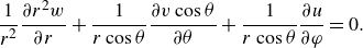(7.1d) \begin{equation}\frac{1}{r^{2}}\frac{\partial r^{2}w}{\partial r}+\frac{1}{r\cos \theta }\frac{\partial v\cos \theta }{\partial \theta }+\frac{1}{r\cos \theta }\frac{\partial u}{\partial \varphi }=0.\end{equation}

The thermodynamic equation for the density will be simplified in consonance with (7.1d ):

(7.1e) \begin{equation}\frac{\partial \rho }{\partial t}+\frac{u}{r\cos \theta }\frac{\partial \rho }{\partial \varphi }+\frac{v}{r}\frac{\partial \rho }{\partial \theta }+w\frac{\partial \rho }{\partial r}=\mathcal{H},\end{equation}

where $\mathcal{H}$ represents all non-adiabatic forcings, such as heating or friction that could lead to changes in density.

Obviously, for gaseous planets a more complex statement of mass conservation and thermal heating would be necessary but (7.1d ) and (7.1e ) are sufficient to illustrate some dynamical novelties for this non-hydrostatic, planetary-scale, dynamics.

To start, let us check on the form that the thermal wind equations take. For the zonal wind, cross-differentiating (7.1a ) and (7.1c ) immediately yields

(7.2) \begin{equation}\sin \theta \frac{\partial u}{\partial r}+\cos \theta \frac{1}{r}\frac{\partial u}{\partial \theta }=\frac{1}{r}\frac{\partial \rho }{\partial \theta }=\frac{\partial u}{\partial s},\end{equation}

as in our previous result, where s is the variable along the rotation axis, whose tilt with respect to the local gravitational vertical is now a function of latitude. The basic result is the same as the quasi-geostrophic one. The same is not true for the meridional velocity.

Cross-differentiating (7.1b ) and (7.1c ) after first multiplying (7.1b ) by r yields

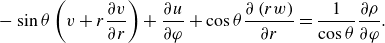(7.3a) \begin{equation}-\sin \theta \left(v+r\frac{\partial v}{\partial r}\right)+\frac{\partial u}{\partial \varphi }+\cos \theta \frac{\partial \left(rw\right)}{\partial r}=\frac{1}{\cos \theta }\frac{\partial \rho }{\partial \varphi }.\end{equation}

Then with use of (7.1d ) , i.e. conservation of mass, we obtain

(7.3b) \begin{equation}\sin \theta \frac{\partial v}{\partial r}+\cos \theta \frac{1}{r}\frac{\partial v}{\partial \theta }=-\frac{1}{r\cos \theta }\frac{\partial \rho }{\partial \varphi }-\cos \theta \frac{w}{r}.\end{equation}

The last term in (7.3b ) is an unexpected one and has no equivalent in the smaller-scale quasi-geostrophic limit. Its origin is the same twisting term in the vector vorticity equation, $(\boldsymbol{\omega }\cdot \nabla )\textbf{u}$ , where now the gradient operates on the unit vectors in spherical coordinates whose derivatives with respect to latitude are different from zero. The final term in (7.3b ) is slightly difficult to interpret but it can be shown to involve tilting of the rotation vector by a component of the radial velocity. For large r the term is generally small because the local surface approaches a flat tangent plane.

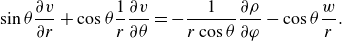
If we now construct the lowest-order vorticity balance by cross-differentiating (7.1a ) and (7.1b ) and using (7.1d ), we easily obtain

(7.4) \begin{equation}v\frac{\cos \theta }{r}=\frac{\sin \theta }{r^{2}}\frac{\partial r^{2}w}{\partial r}+\frac{1}{r\cos \theta }\frac{\partial w(\cos \theta )^{2}}{\partial r},\end{equation}

or, carrying out the differentiation in (7.4),

(7.5) \begin{equation}v\frac{\cos \theta }{r}=\sin \theta \frac{\partial w}{\partial r}+\cos \theta \frac{1}{r}\frac{\partial w}{\partial \theta }=\frac{\partial w}{\partial s},\end{equation}

which we recognize as the non-dimensional form of the vorticity equation in which vortex stretching along the rotation axis leads to northward motion on the beta plane, but here on the spherical pathway in the planet’s fluid envelope.

The content of (7.5) is, again, slightly richer. The first term on the right-hand side of (7.5) is clearly the traditional production of vorticity by stretching along the axis of the fluid column oriented in the radial direction and producing vorticity by the stretching of the local vertical component of the planetary vorticity. However, the second term on the right-hand side of (7.5) is a tilting term. The horizontal variation of w in the meridional direction will tilt that component into the vertical direction, adding (or subtracting) that effect from the stretching term. The sum of the two produces a northward or southward movement due to the beta effect, the term on the left-hand side of (7.5).

Further, (7.1a ) and (7.1c ) together imply that

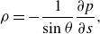(7.6) \begin{equation}\rho =-\frac{1}{\sin \theta }\frac{\partial p}{\partial s},\end{equation}

as in the quasi-geostrophic limit.

Ertel’s theorem, i.e. the equation for the potential voriticity, follows from the above relations. As shown in Pedlosky (Reference Pedlosky1986), if a function $\lambda$ can be written as a function of p and $\rho$ then the vorticity equation can be written as an equation for the potential vorticity, $q=\omega _{a}\cdot \nabla \lambda$ , where, in the case at hand, $\omega _{a}$ is simply, in dimensional units, $2\vec {\varOmega }$ . In the case discussed here, the density itself can be chosen to take the role of $\lambda$ , so that the potential vorticity $\boldsymbol{\omega }_{\boldsymbol{a}}\cdot \nabla \boldsymbol{\rho }$ is, in our non-dimensional units, just

(7.7) \begin{equation}q=\frac{\partial \rho }{\partial s}\end{equation}

and its governing equation is

(7.8) \begin{equation}\frac{\partial }{\partial t}\frac{\partial \rho }{\partial s}+\frac{u}{r\cos \theta }\frac{\partial }{\partial \varphi }\left(\frac{\partial \rho }{\partial s}\right)+v\frac{1}{r}\frac{\partial }{\partial \theta }\left(\frac{\partial \rho }{\partial s}\right)+w\frac{\partial }{\partial r}\left(\frac{\partial \rho }{\partial s}\right)=0.\end{equation}

In (7.8) $u\ \textrm{and}\ \rho$ can be written directly in terms of the pressure p and its derivatives, while w is related to v via (7.5). But these relationships are not easy and the system as a whole is difficult to work with.

8. An example

Some progress can be made, however. Combining (7.1b ) and (7.5) leads to

(8.1) \begin{equation}\frac{\partial w}{\partial s}-\frac{(\cos \theta )^{2}}{\sin \theta }w=\frac{1}{r\sin \theta }\frac{\partial p}{\partial \varphi }.\end{equation}

If we consider the special case where the radial density gradient is determined by other thermodynamic processes, this leads to a large radial density gradient existing in the absence of motion such that the dominant density gradient is radial and

(8.2) \begin{equation}\frac{\partial \rho _{o}}{\partial r}=S.\end{equation}

Where that radial gradient exceeds in magnitude all perturbations of the density $\rho$ , the linear governing equation would be simply

(8.3) \begin{equation}\frac{\partial \rho }{\partial t}+wS=0.\end{equation}

Using (8.1), (8.2) and (8.3) we obtain

(8.4) \begin{equation}\frac{\partial }{\partial t}\left[\frac{\partial }{\partial s}\frac{1}{S}\left(\frac{\partial p}{\partial s}\right)+\frac{(\cos \theta )^{2}}{\sin \theta }\frac{\frac{\partial p}{\partial s}}{S}\right]=-\frac{1}{r\sin \theta }\frac{\partial p}{\partial \varphi }.\end{equation}

Roughly speaking, (8.4) recalls the form of the potential vorticity equation of § 2 except that on these scales the relative vorticity of the background flow is negligible in comparison with the planetary vorticity gradient. Motion in that field is given by the term on the right-hand side of (8.4) while the potential vorticity is dominated by the stretching of the planetary vorticity, the rate of change of which is given by the left-hand side of (8.4).

If the pressure field is expanded in a series, then

(8.5) \begin{equation}p=\sum _{n}F_{n}(s)\varPsi_{n}(\varphi ,t),\end{equation}

where the functions $F_{n }$ satisfy

(8.6) \begin{equation}\frac{\partial }{\partial s}\frac{1}{S}\left(\frac{\partial F_{n}}{\partial s}\right)+\frac{(\cos \theta )^{2}}{\sin \theta }\frac{\frac{\partial }{\partial s}F_{n}}{S}=-{\lambda _{n}}^{2}F_{n},\end{equation}

leading to

(8.7) \begin{equation}\frac{\partial \varPsi_{n}}{\partial t}=-\frac{1}{{r\cos \theta \lambda _{n}}^{2}}\frac{\partial \varPsi_{n}}{\partial \varphi }.\end{equation}

This leads to propagation of this long wave always westward. Note that in this formulation latitude is a parameter of the motion.