


1. Introduction
We consider a gravity-driven two-dimensional liquid film falling down a plane tilted at an angle  $\phi$ with respect to the horizontal, in contact with a counter-current gas flow that is strongly confined by an upper wall placed at
  $y=H$ (figure 1). Both fluids are Newtonian, with constant fluid properties, and the flow is laminar. Confined falling liquid films occur in rectification columns for cryogenic air separation, which contain structured packings that subdivide the column cross-section into millimetric channels (Valluri et al. Reference Valluri, Matar, Hewitt and Mendes2005). Even stronger confinement is realized in compact reflux condensers (Vlachos et al. Reference Vlachos, Paras, Mouza and Karabelas2001), falling-film microreactors (Zhang et al. Reference Zhang, Chen, Yue and Yuan2009) and micro-gap coolers (Kabov et al. Reference Kabov, Zaitsev, Cheverda and Bar-Cohen2011). We are interested in nonlinear waves that form on the surface of the falling liquid film due to the long-wave Kapitza instability (Kapitza Reference Kapitza1948), and, in particular, how these are affected by the gas velocity in a strongly confined setting. Such waves are known to trigger flooding events, by local obstruction of the channel, by flow reversal or by wave reversal (Vlachos et al. Reference Vlachos, Paras, Mouza and Karabelas2001; Trifonov Reference Trifonov2010a; Tseluiko & Kalliadasis Reference Tseluiko and Kalliadasis2011).

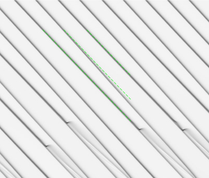
Figure 1. Problem sketch: gravity-driven falling liquid film (lower blue streamlines) in contact with a counter-current gas flow (upper red streamlines) flowing through a channel of dimensional gap height  $H^\star$ inclined at an angle
  $\phi$ with respect to the horizontal. Streamlines (separated by constant streamfunction increments) are shown in the wall-fixed reference frame, and
  $\varLambda$ is the wavelength.
For weak confinements, flooding seems to be favoured by decreasing the gap height and/or increasing the gas flow rate. Experiments (Kofman, Mergui & Ruyer-Quil Reference Kofman, Mergui and Ruyer-Quil2017) and numerical simulations (Trifonov Reference Trifonov2010a,Reference Trifonovb) alike have shown that the amplitude of nonlinear waves increases with increasing counter-current gas flow, and that this growth diverges in the vicinity of the flooding point (Drosos, Paras & Karabelas Reference Drosos, Paras and Karabelas2006). Moreover, actual flooding experiments have shown that the critical gas flow rate decreases with diminishing gap height (Sudo Reference Sudo1996). Linear stability investigations, which demonstrate an increase in the maximal linear growth rate with increasing gas velocity, tend to confirm this nonlinear picture (Alekseenko et al. Reference Alekseenko, Aktershev, Cherdantsev, Kharlamov and Markovich2009; Vellingiri, Tseluiko & Kalliadasis Reference Vellingiri, Tseluiko and Kalliadasis2015; Schmidt et al. Reference Schmidt, Náraigh, Lucquiaud and Valluri2016; Trifonov Reference Trifonov2017).
On the other hand, recent investigations suggest that strong confinements may, in fact, lower the risk of flooding. Lavalle et al. (Reference Lavalle, Li, Mergui, Grenier and Dietze2019) have shown that the Kapitza instability can be entirely suppressed by sufficiently confining the gas, as suggested by Tilley, Davis & Bankoff (Reference Tilley, Davis and Bankoff1994) and confirmed by Kushnir et al. (Reference Kushnir, Barmak, Ullmann and Brauner2021), and that this is facilitated by low tilt angles. Further, the authors observed that the linear stabilization, which they confirmed experimentally, is amplified by increasing the counter-current gas flow rate. Recent nonlinear direct numerical simulations (DNS) of inclined falling liquid films (Trifonov Reference Trifonov2020) have identified a non-monotonic variation of the interfacial velocity, mean film thickness and inter-phase friction coefficient with increasing counter-current gas velocity, although the trend of the wave amplitude remained monotonic and increasing.
These investigations have motivated us to take a closer look at strongly confined inclined falling liquid films, in contrast to Dietze & Ruyer-Quil (Reference Dietze and Ruyer-Quil2013) and Lavalle et al. (Reference Lavalle, Grenier, Mergui and Dietze2020), who studied the vertical configuration, where the gas-induced linear stabilization is relatively weak. This is because the inertia-induced destabilizing mechanism of the Kapitza instability is weakened less and less by the stabilizing effect of normal gravity as the tilt angle is increased, and thus the relative weight of the gas effect diminishes (Lavalle et al. Reference Lavalle, Li, Mergui, Grenier and Dietze2019). We aim to confront linear stability predictions with the response of nonlinear surface waves to an increasingly strong counter-current gas flow. In particular, we wish to know whether nonlinear travelling waves can be damped under the effect of the gas flow, in line with the linear observations, and, if so, whether they may resist secondary instability. Such a situation would amount to a reduced flooding risk. By secondary instability we mean the loss of stability of travelling-wave solutions (TWS) produced by the primary Kapitza instability (Liu & Gollub Reference Liu and Gollub1993; Lavalle et al. Reference Lavalle, Grenier, Mergui and Dietze2020), and our analysis is restricted to two-dimensional such instability modes.
An enticing preliminary result was obtained by Samanta (Reference Samanta2014), who showed that applying a constant interfacial shear stress to an inclined wavy falling liquid film can strongly reduce the amplitude of nonlinear surface waves. However, for the strong confinement studied here, variations of the shear stress with wave height play an important role (Lavalle et al. Reference Lavalle, Li, Mergui, Grenier and Dietze2019), and the gas pressure gradient, which was also neglected in the model of Samanta (Reference Samanta2014), needs to be accounted for (Dietze & Ruyer-Quil Reference Dietze and Ruyer-Quil2013).
To tackle this problem, we use the two-phase weighted residual integral boundary layer (WRIBL) model of Dietze & Ruyer-Quil (Reference Dietze and Ruyer-Quil2013) to construct TWS, with the continuation software ‘Auto07P’ (Doedel Reference Doedel2008), and to compute spatially evolving wavy falling liquid films, with our own finite-difference code (Lavalle et al. Reference Lavalle, Grenier, Mergui and Dietze2020). These nonlinear computations are confronted with linear stability calculations based on the WRIBL model, and solutions of the full Orr–Sommerfeld (OS) eigenvalue problem (Tilley et al. Reference Tilley, Davis and Bankoff1994), whereby we have employed a spatial stability formulation (Barmak et al. Reference Barmak, Gelfgat, Vitoshkin, Ullman and Brauner2016). Also, we check for periodic secondary instabilities via transient periodic computations started from TWS (Lavalle et al. Reference Lavalle, Grenier, Mergui and Dietze2020), and confront our model with a DNS based on the full Navier–Stokes equations, using the finite-volume solver ‘Basilisk’ (Popinet Reference Popinet2015).
Our paper is structured as follows. The mathematical description and numerical methods are introduced in § 2, followed by § 3, which reports results of our linear and nonlinear computations. Then, § 3.1 is dedicated to surface waves of the linearly most-amplified frequency, whereas § 3.2 concerns low-frequency solitary waves (here, we will also introduce our DNS data). Conclusions are drawn in § 4.
2. Mathematical description
The flow in figure 1 is governed by the Navier–Stokes and continuity equations, written in Einstein notation using the directional indices  $i=1,2$ and
  $j=1,2$ (
 $x_1=x,\ u_1=u,\ x_2=y$ and
  $u_2=v$), and the phase indicator
  $m$, which identifies liquid (
 $m = l$) and gas (
 $m = g$):
 $$\begin{gather} {X_m\partial_{t} {u}_i}+{u}_j \partial_{{x}_j}{u}_i={-}\partial_{{x}_i}{p_m} + {{Re}_m^{{-}1}} \partial_{{x}_j{x}_j}{u}_i +X_m^2{Fr}^{{-}2}\{\delta_{i1}\sin(\phi)-\delta_{i2}\cos(\phi)\}, \end{gather}$$
 $$\begin{gather}\partial_{{x}_j}{u}_j=0, \end{gather}$$
where lengths have been scaled with the channel height  $\mathcal {L} = H^\star$ (stars denote dimensional quantities throughout), velocities with the phase-specific signed superficial velocities
  $\mathcal {U}_m = q_{m0}^\star$/
 $H^\star$, time with
  $\mathcal {T} = \mathcal {L}$/
 $\mathcal {U}_l$, and the phase-specific pressure
  $p_m$ with
  $\rho _m\mathcal {U}_m^2$. Further,
  $\delta _{ij}$ is the Kronecker symbol,
  $X_l = 1$ and
  $X_g = \mathcal {U}_l/\mathcal {U}_g$. The gravitational acceleration
  $g$ enters through the Froude number
  ${Fr} = \mathcal {U}_l$/
 $\sqrt {g\mathcal {L}}$, and the Reynolds numbers
  ${Re}_m = \mathcal {U}_m\mathcal {L}({\rho _m}/{\mu _m}) = q_{m0}^\star ({\rho _m}/{\mu _m})$ are based on the phase-specific signed nominal flow rates
  $q_{m0}^\star$ of the flat-film primary flow,
  $q^\star _{g0}$ and
  ${Re}_g$ being negative for a counter-current gas flow. The boundary conditions are
 $$\begin{gather} {u_{l}}|_{y=0}= {v_{l}}|_{y=0}= {u_{g}}|_{y=1}= {v_{g}}|_{y=1}=0, \end{gather}$$
and the kinematic and dynamic coupling conditions at the film surface  $y = h(x,t)$,
 $$\begin{gather} {u}_{l}=X_g^{{-}1}{u}_{g},\quad {v}_{l}=X_g^{{-}1}{v}_{g}=\partial_{{t}}{h}+{{u}_{l}} \partial_{{x}}{h}, \end{gather}$$
 $$\begin{gather}p_l+[{S}^{l}_{ij} n_j] n_i=X_g^{{-}2}\varPi_{\rho} p_g+{X_g^{{-}1}\varPi_{\mu}}[{S}^{ g}_{ij} n_j] n_i+{We} \,{\kappa}, \end{gather}$$
 $$\begin{gather}[{S}^{ l}_{ij} n_j] \tau_i=X_g^{{-}1}\varPi_{\mu}[{S}^{ g}_{ij} n_j] \tau_i, \end{gather}$$
where  $S^{m}_{ij} = \frac {1}{2}(\partial _{x_j} u_i+\partial _{x_i} u_j)$ denotes the strain-rate tensor,
  $\varPi _\mu = \mu _g/\mu _l$ and
  $\varPi _\rho = \rho _g/\rho _l$ are the dynamic viscosity and density ratios, and the surface tension
  $\sigma$ enters through the Weber number
  ${We} = \sigma \rho _l^{-1}\mathcal {U}_l^{-2}\mathcal {L}^{-1}$. The orthonormal surface coordinate system is constructed by
  $\boldsymbol {n} = [{-{\partial _x h }, 1} ]( {1+{\partial ^2_x h } } )^{ - 1/2}$ and
  $\boldsymbol {\tau } = [ {1, {\partial _x h }} ]( {1 + {\partial ^2_x h } } )^{ - 1/2}$, from which we obtain the film surface curvature
  ${\kappa } = -\boldsymbol {\nabla }\boldsymbol {\cdot }\boldsymbol {n}$.
We perform two types of calculations based on the first principles (2.1) to validate our low-dimensional model. First, we solve the OS linear stability problem (Tilley et al. Reference Tilley, Davis and Bankoff1994), assuming spatially growing normal modes (Barmak et al. Reference Barmak, Gelfgat, Vitoshkin, Ullman and Brauner2016):
 \begin{equation} \begin{bmatrix} h\\ \varPhi\\ \varPsi\\ p_m \end{bmatrix}= \begin{bmatrix} h_0\\ \varPhi_0(y)\\ \varPsi_0(y)\\ p_{m0}(x,y) \end{bmatrix} + \begin{bmatrix} \hat{h}\\ \phi(y)\\ \psi(y)\\ \hat{p}_m(y) \end{bmatrix}\exp\{\textrm{i}(kx-\omega t)\}, \end{equation}
where  $\varPhi$ and
  $\varPsi$ designate the streamfunctions in the liquid and gas, the subscript
  $0$ denotes the flat-interface base flow,
  $k\in \mathbb {C}$ is the complex wavenumber of the perturbation and
  $\omega \in \mathbb {R}$ is its angular frequency. We focus on long-wave instability modes, which we track through numerical continuation using Auto07P (Lavalle et al. Reference Lavalle, Li, Mergui, Grenier and Dietze2019), having checked with a Chebyshev collocation code (Barmak et al. Reference Barmak, Gelfgat, Vitoshkin, Ullman and Brauner2016) that short wave modes remain stable throughout the studied parameter range. Second, we perform a DNS with the finite-volume solver Basilisk (Popinet Reference Popinet2015), based on the volume-of-fluid (VOF) and the continuum surface force (CSF) methods, following (Dietze Reference Dietze2019). Here, we impose periodic conditions on a domain spanning the wavelength
  $\varLambda$.
Our low-dimensional model is based on the WRIBL approach (Ruyer-Quil & Manneville Reference Ruyer-Quil and Manneville1998; Kalliadasis et al. Reference Kalliadasis, Ruyer-Quil, Scheid and Velarde2012), which describes the flow via evolution equations for the flow rate  $q$ and film height
  $h$. We employ the two-phase formulation of Dietze & Ruyer-Quil (Reference Dietze and Ruyer-Quil2013) written in Einstein notation (
 $m = l,g$ and
  $n = l,g$):
 $$\begin{gather} \{S_m \partial_t q_m + F_{mn} q_m\partial_x q_n+G_{mn} q_{j}q_{m}\partial_x h\}\nonumber\\ \quad ={-}{We}\,\partial_{xxx} h +{Fr}^{{-}2}( 1-\varPi_\rho ) \{\sin(\phi)-\cos(\phi)\partial_xh\}+ {Re}_m^{{-}1}C_{m}q_m\nonumber\\ \qquad +{Re}_m^{{-}1}\{J_m q_m ( \partial_x h) ^2 + K_m \partial_x q_m \partial_x h + L_m q_m \partial_{xx} h + M_m \partial_{xx} q_m\}, \end{gather}$$
 $$\begin{gather} \partial_x q_l+\partial_t h=0,\quad \partial_x q_g-X_g\partial_t h=0,\end{gather}$$
where  $q_l$ and
  $q_g$ denote the liquid and gas flow rates (per unit width) and the coefficients
  $S_m$,
  $F_{mn}$,
  $G_{mn}$,
  $C_{mn}$,
  $J_n$,
  $K_n$,
  $L_n$ and
  $M_n$ are known functions of the film height
  $h$ (Dietze & Ruyer-Quil Reference Dietze and Ruyer-Quil2013).
We perform linear stability calculations by solving the dispersion equation  ${DR}(\omega ,k)=0$, obtained by linearizing (2.3) around
  $[h_0,q_{l0},q_{g0}]$, for
  $k = k_r+\textrm {i}k_i$ at a given
  $\omega \in \mathbb {R}$:
 $$\begin{gather} [h,q_l,q_g]^\textrm{T}=[h_0,q_{0l},q_{0g}]^\textrm{T}+[\hat{h},\hat{q}_{l},\hat{q}_{g}]^\textrm{T} \exp\{\textrm{i}(kx-\omega t)\}, \end{gather}$$
 $$\begin{gather} {DR}=\textrm{i}\omega^2\{S_g-S_l\}+\textrm{i}k\omega \{F_{ml}q_m-F_{mg}q_m\}+\textrm{i}k^2G_{mn}q_mq_n\nonumber\\ \quad +\textrm{i}k^2{Fr}^{{-}2}\{\cos(\phi)-\varPi_\rho\cos(\phi)\}-i^3k^4{We} +\omega\{{Re}_g^{{-}1}C_g-{Re}_l^{{-}1}C_l\}\nonumber\\ \quad -k{Re}_m^{{-}1}\partial_h C_mq_m-i^2k^3{Re}_m^{{-}1}L_mq_m +i^2k^2\omega\{{Re}_g^{{-}1}M_g-{Re}_l^{{-}1}M_l\}. \end{gather}$$
We also compute nonlinear TWS, which remain unaltered in a reference frame moving at the wave speed  $c$, through numerical continuation based on (2.3), using Auto07P (Doedel Reference Doedel2008). Our code allows us to track TWS at the linearly most-amplified angular frequency
  $\omega = \omega _{max}$, via the following constraints (Dietze, Lavalle & Ruyer-Quil Reference Dietze, Lavalle and Ruyer-Quil2020):
 \begin{equation} {DR}(\omega_{max},k)=0, \quad {\partial_\omega k_i}|_{\omega=\omega_{max}}=0. \end{equation}
Finally, we check the stability of nonlinear TWS via transient computations based on (2.3), using either periodic or inlet/outlet boundary conditions (Lavalle et al. Reference Lavalle, Grenier, Mergui and Dietze2020).
3. Results
We set the tilt angle to  $\phi = 10^\circ$ and focus on a single fluid combination, a 83 % by weight aqueous dimethylsulfoxide (DMSO) solution used in experiments (Dietze, Al-Sibai & Kneer Reference Dietze, Al-Sibai and Kneer2009), where
  $\rho _l=1098.3$ kg m
 $^{-3}$,
  $\mu _l = 3.13$ mPa s and
  $\sigma =0.0484$ N m
 $^{-1}$, in contact with ambient air. The Kapitza number for this combination is
  ${Ka} = \sigma \rho _l^{-1/3}g^{-1/3}\mu _l^{-4/3}=509.5$. The channel height
  $H^\star$ is varied as
  $H^\star =1.2$, 1.7, 1.8, 1.9, 2.1 and 2.4 mm, which corresponds to values of
  $\eta =2$, 2.8, 3, 3.1, 3.4 and 3.9 for the relative confinement:
 \begin{equation} {\eta=H^\star{/} {h^\star_0}|_{M=1}=1/ {h_0}|_{M=1},} \end{equation}
where  ${h_0}|_{M=1}$ is the primary flow film thickness for an aerostatic gas pressure gradient, i.e.
  $M = {\partial _xp_g}/{\sin (\phi )}=1$. We wish to confront the linear and nonlinear implications of increasing the counter-current gas flow rate at fixed
  ${Re}_l$. In particular, we wish to know whether nonlinear waves can be damped via increasing
  $|{Re}_g|$.
3.1. Most-amplified waves
Figure 2 demonstrates the effect of increasing the counter-current gas flow rate on the linearly most-amplified waves ( $\omega =\omega _{max}$) at fixed
  ${Re}_l=15$ for different
  $\eta$ values. Along each curve in figures 2(a) and 2(c), the channel height
  $H^\star$ remains fixed while
  $h_0$ increases (between 10 % for the strongest and 20 % for the weakest confinement), and so
  $\eta$ (3.1) specifies a representative confinement for each case, corresponding to the rightmost point of each curve (where
  $M=1$). Curves in figure 2(a) track the maximum linear spatial growth rate
  $-k_i^{max}$ in terms of
  ${Re}_g$, dashed lines corresponding to OS and solid lines to WRIBL calculations. At the largest
  $\eta$ (filled squares,
  $\eta =3.9$), the growth rate increases monotonically with
  $|{Re}_g|$, implying a gas-induced destabilization, up to the onset of absolute instability (AI), where
  $-k_{i max}$ diverges (Vellingiri et al. Reference Vellingiri, Tseluiko and Kalliadasis2015). Conversely, at very small
  $\eta$ values (open squares and pentagons,
  $\eta =2$, 2.8), the effect of the gas is monotonically stabilizing, up to the point of fully suppressing (S) the long-wave Kapitza instability (Lavalle et al. Reference Lavalle, Li, Mergui, Grenier and Dietze2019; Kushnir et al. Reference Kushnir, Barmak, Ullmann and Brauner2021). In the intermediate range (crosses, asterisks and diamonds,
  $\eta =3$, 3.1 and 3.4), the behaviour is non-monotonic, stabilization occurring at low and destabilization at large values of
  $|{Re}_g|$. Figures 2(b) (
 $\eta =3.1$) and 2(d) (
 $\eta =2$) represent dispersion curves for the non-monotonic and fully stabilizing cases. Overall, there is quantitative agreement for
  $|{Re}_g| < 150$ between linear OS and WRIBL predictions in figures 2(a), 2(b) and 2(d), whereas qualitative agreement is retained when approaching the AI limits.

Figure 2. Most-amplified waves:  $\phi = 10^\circ$,
  ${Re}_l=15$,
  ${Ka}=509.5$. Linear (a,b,d) versus nonlinear (c) predictions. Filled squares,
  $\eta =3.9$; diamonds,
  $\eta =3.4$; asterisks,
  $\eta =3.1$; crosses,
  $\eta =3$; pentagons,
  $\eta =2.8$; open squares,
  $\eta =2$. (a) Maximal linear growth rate
  $-k_i^{max}$ versus
  ${Re}_g$, related to the aerostatic limit
  $\{-k_i^{max}\}_{M=1}$, where
  $M = {\partial _xp_g}/{\sin (\phi )}$. Solid, WRIBL; dashed, OS. (b,d) Dispersion curves
  $-k_i(\omega )$ for two cases from panel (a). Red curves trace
  $-k_i^{max}(\omega _{max})$ up to absolute instability (AI) or full stabilization (S). (b) For
  $\eta =3.1$, from right to left:
  $M=1$,
  ${Re}_g=-60$,
  $-100$,
  $-145$,
  $-170$ and
  $-184$. (d) For
  $\eta =2$, from right to left:
  $M=1$,
  ${Re}_g=-4$,
  $-7$ and
  $-10$. (c) Amplitude of nonlinear TWS (WRIBL) at
  $\omega = \omega _{max}$. PH denotes period-halving bifurcations and dot-dashed green lines identify periodically unstable TWS.
Figure 2(c) plots the upper and lower relative film height deflections  $h_{max}/\bar {h}-1$ and
  $h_{min}/\bar {h}-1$ for nonlinear TWS at
  $\omega = \omega _{max}$, where
  $\bar {h} = \varLambda ^{-1}\int _0^\varLambda h \,{\textrm {d} x}$ is the film height averaged over one wavelength, with
  $\bar {h}\neq h_0$ in the case of nonlinear waves. For
  $\eta =3$, 3.1 and 3.4, TWS display a non-monotonic trend that is opposed to the linear one. That is,
  $h_{max}/\bar {h}-1$ in figure 2(c), which we will refer to as the wave amplitude, first increases and then decreases with increasing
  $|{Re}_g|$, whereas
  $-k_i^{max}$/
 $\{-k_i^{max}\}_{M=1}$ in figure 2(a) first decreases and then increases. Conversely, for
  $\eta =2$ and 2.8, the nonlinear and linear trends both imply stabilization, and, for
  $\eta =3.9$, they both imply destabilization, at least up to the amplitude maximum in figure 2(c). Except for the two weakest confinements (
 $\eta =2$, 2.8, 3 and 3.1), TWS are bounded by a nonlinear wave suppression, where
  $h_{max} = h_{min}$, resulting from period-halving (PH) bifurcations (marked by symbols), which sets in before the linear AI and S thresholds in figure 2(a). Figure 3(a) shows wave profiles leading up to such a PH bifurcation (
 $\eta =3$). The sole precursory capillary ripple is seen to grow until splitting the wave into two identical halves. Conversely, for
  $\eta =3.9$ (figure 3b), the capillary ripple disappears when increasing
  $|{Re}_g|$ towards the AI limit.

Figure 3. Wave profiles of TWS from figure 2(c). (a) For  $\eta =3$ (cross in figure 2c). Approaching the PH bifurcation:
  ${Re}_g=-37$ (thick solid) to
  ${Re}_g=-88$ (green). (b) For
  $\eta =3.9$ (filled square in figure 2c). Suppression of the capillary ripple while approaching the AI limit:
  ${Re}_g=-79$ (thick solid) to
  ${Re}_g=-348$ (green).
We conclude from figure 2 that linear stability predictions can be misleading. In particular, the amplitude of nonlinear waves may grow with increasing counter-current gas velocity, even though the linear growth rate decreases. Further, TWS become unstable to periodic secondary instability modes (dot-dashed lines in figure 2c) beyond a threshold  ${Re}_g$, which we have determined via transient periodic computations started from TWS. These periodic modes do not lead to dangerous events, but TWS are also prone to a subharmonic instability in the case of a spatially evolving film (see supplementary movie 1 available at https://doi.org/10.1017/jfm.2021.417). Originally identified in unconfined films (Liu & Gollub Reference Liu and Gollub1993), this instability triggers wave coalescence events (Chang, Demekhin & Kalaidin Reference Chang, Demekhin and Kalaidin1996a) that can lead to intermittent flooding in long channels (Dietze & Ruyer-Quil Reference Dietze and Ruyer-Quil2013).
3.2. Solitary waves
We focus now on low-frequency solitary waves at a fixed wavelength  $\varLambda =4.5\tilde {\varLambda }_{max}$, where
  $\tilde {\varLambda }_{max}$ denotes the linearly most-amplified wavelength for a passive outer phase, all other parameters remaining as in figure 2. These waves lie on the ascending branch of the linear dispersion curves in figures 2(b) and 2(d), and thus the linear effect of increasing the gas flow is monotonic, either destabilizing (
 $\eta =3$, 3.1, 3.4 and 3.9) or stabilizing (
 $\eta =2$ and 2.8). Figure 4(a) represents the nonlinear response of solitary TWS, evidencing a monotonic gas-induced attenuation of the wave amplitude for
  $\eta =2$, 2.8, 3 and 3.1. For
  $\eta =3$ and 3.1, this nonlinear effect is opposed to the linear amplification, and both effects are inverted with respect to the initial response of the most-amplified waves (figure 2a,c). Solution branches of solitary TWS in figure 4(a) are bounded either by the linear thresholds of absolute instability (AI,
  $\eta =3$, 3.1 and 3.4) and full stabilization (S,
  $\eta =2$ and 2.8) from figure 2(a), or by a nonlinear limit point (LP,
  $\eta =3.9$) that occurs slightly before (about 2 % in terms of
  $Re _g$) the AI bound.

Figure 4. Solitary waves:  $\phi = 10^\circ$,
  ${Re}_l=15$,
  ${Ka}=509.5$,
  $\varLambda =4.5\tilde {\varLambda }_{max}$. (a) Amplitude of nonlinear TWS (WRIBL). Right to left:
  $\eta =2, 2\ (\varPi _\mu =0), 2\ (\varPi _\rho =0),\ 2.8,\ 3,\ 3.1,\ 3.4$ and 3.9. Dot-dashed green lines highlight periodically unstable solutions. (b) Wave profiles corresponding to open circles (
 $\eta =3.9$) in panel (a). Bottom to top:
  ${Re}_g=-10$,
  $-$100,
  $-$145 and
  $-$149. (c) Transient periodic computation started from thick-solid TWS in panel (b). Black, local film height; green, wave height. (d) Flat-top wave corresponding to black filled circle in figure 4(a):
  $\eta =2$,
  ${Re}_g=-7$. Streamlines in the wave-fixed reference frame. (e) Different limits of the
  $\eta =2$ solution in panel (d) (filled circles in panel a). Solid black, full inter-phase coupling; dashed blue,
  $\varPi _\mu =0$ in (2.1e) and (2.1f); dot-dot-dashed red,
  $\varPi _\rho =0$ in (2.1e); open circles, DNS at
  $M = {\partial _xp_g}/{\sin (\phi )} = M_{TWS}=84.8$,
  ${Re}_l=15.7$.
For the strongest confinement,  $\eta =2$ (open squares in figure 4a), linear and nonlinear effects are aligned and stabilizing. In that case, the gas shapes the wave hump into an elongated flat-top form (figure 4d). In figure 4(e), we compare this solution (solid line) with TWS in the limits
  $\varPi _\rho =0$ (red dot-dot-dashed) and
  $\varPi _\mu =0$ (blue dashed), which respectively deactivate the gas pressure and the gas-side viscous stresses in (2.1e) and (2.1f). From this comparison, we can conclude that the gas pressure gradient and not the gaseous viscous stresses are the cause for wave flattening. The flat-top TWS (also shown in figure 1), which we have reproduced with a DNS at slightly greater
  ${Re}_l=15.7$ (open circles in figure 4e), is stable in periodic transient computations, and undergoes only weak modulations in a spatially evolving film (see supplementary movie 2).
For the weakest confinement,  $\eta =3.9$, solitary TWS are more susceptible to secondary instability modes. We discuss this based on the wave profiles in figure 4(b), which correspond to the TWS marked by open circles in figure 4(a). The TWS at
  ${Re}_g=-145$ (thick solid profile in figure 4b, second from left open circle in figure 4a) still lies on the periodically stable solution branch (solid curve in figure 4a). For this case, secondary instability can only arise through wave interactions. Pradas et al. (Reference Pradas, Kalliadasis, Nguyen and Bontozoglou2013) showed, for the case of a passive atmosphere, that solitary waves can develop such interactions via the precursory capillary ripples, leading to oscillations around bound states, where neighbouring waves repeatedly approach and recoil from one another. Thereby, the approaching wave always grows, whereas the slowing wave always diminishes, in amplitude. In the presence of a counter-current gas flow, we observe a secondary instability mode that involves a different wave interaction. We demonstrate this through an open-domain computation with coherent inlet forcing at the TWS frequency
  $f = {2{\rm \pi} }/{\omega } = \,f_{TWS}=0.20$. Figures 5(a) and 5(b) (see also supplementary movie 3) show that the instability produces solitary waves of diminishing amplitude that accelerate in the slipstream of their growing leading neighbours. This clearly differs from the behaviour of unconfined falling films, such as the above-mentioned oscillations around bound states (Pradas et al. Reference Pradas, Kalliadasis, Nguyen and Bontozoglou2013) or the well-known coarsening dynamics (Chang et al. Reference Chang, Demekhin, Kalaidin and Ye1996b), where larger-amplitude waves catch up with and accumulate the smaller ones travelling in front. The slipstreaming occurs in concert up- and downstream of a leading wave, and thus the latter is increasingly exposed to the counter-current gas flow, leading eventually to its destruction through a wave breaking event, before coalescence can occur.

Figure 5. Slipstreaming (a,b) and wave splitting (c,d) in solitary wave trains. Spatio-temporal computations with our WRIBL model (2.3) on an open domain of length  $L = 31.4 \varLambda _{TWS}$, applying coherent inlet forcing at
  $f = \,f_{TWS}$:
  $\phi = 10 ^\circ$,
  $\eta =3.9$,
  ${Re}_l=15$,
  ${Ka}=509.5$. Space–time plots of the film height
  $h$ (a,c), and wave profile snapshots (b,d). Parallel green dashed lines indicate initial TWS celerity. (a,b) For
  ${Re}_g=-145$,
  $\,f_{TWS}=0.20$. (c,d) For
  ${Re}_g=-149$,
  $\,f_{TWS}=0.19$. Red symbols identify primary/secondary wave maxima.
When increasing the counter-current gas velocity further, TWS become periodically unstable (dot-dashed branches in figure 4a). For the TWS at  $\eta =3.9$ and
  ${Re}_g=-149$ (thin solid profile in figure 4b, leftmost open circle in figure 4a), the instability leads to a self-sustained repeated breaking and reconstructing of the wave crest, as shown in figure 4(c) via a transient computation with periodicity conditions started from the TWS. In a spatially evolving film, which we have mimicked through an open-domain computation with inlet forcing frequency
  $f = \,f_{TWS}=0.19$ (figure 5c,d, and see supplementary movie 4), the instability leads to ubiquitous wave splitting events that refine the solitary wave train into a train of shorter and smaller daughter waves. This gas-induced refining dynamics can be viewed as the opposite of the coarsening dynamics observed in unconfined films (Chang et al. Reference Chang, Demekhin, Kalaidin and Ye1996b). We point out that isolated wave splitting events have been observed in noise-driven wave regimes, both experimentally (Kofman et al. Reference Kofman, Mergui and Ruyer-Quil2017) and numerically (Dietze & Ruyer-Quil Reference Dietze and Ruyer-Quil2013).
4. Conclusion
In this work, we have demonstrated that linear stability predictions of strongly confined falling liquid films can mislead in estimating the effect of a counter-current gas flow on the film's waviness. Both for waves of the most amplified frequency and for low-frequency solitary waves, we have identified situations where the linear and nonlinear responses are opposed, i.e. linear waves are damped while nonlinear ones are amplified, or vice versa. In some cases, linear waves are bounded by absolute instability, whereas nonlinear waves are fully suppressed via a period-halving bifurcation. Nonetheless, at very strong confinement, both the linear and nonlinear responses imply stabilization and TWS resist secondary instability. This suggests that the risk of wave-induced flooding can be lowered by strongly confining the flow. At weaker confinement, we have found two new secondary instability modes not observed in unconfined films. The first tends to coarsen the wave train, via smaller waves accelerating in the slipstream of their leading neighbours. The second causes wave splitting events that refine the wave train into a sequence of less dangerous shorter and smaller daughter waves.
Our two-dimensional analysis cannot account for the spanwise destabilization of TWS, which entails the formation of three-dimensional waves in the downstream portion of a spatially evolving falling liquid film (Chang Reference Chang1994; Liu, Schneider & Gollub Reference Liu, Schneider and Gollub1995; Scheid, Ruyer-Quil & Manneville Reference Scheid, Ruyer-Quil and Manneville2006; Dietze et al. Reference Dietze, Rohlfs, Nährich, Kneer and Scheid2014; Kofman, Mergui & Ruyer-Qui Reference Kofman, Mergui and Ruyer-Qui2014; Kharlamov et al. Reference Kharlamov, Guzanov, Bobylev, Alekseenko and Markovich2015). Nonetheless, we expect our conclusion on the stabilizing effect of strong confinement to extend to that situation. Firstly, the inertia-driven three-dimensional secondary instability mode (Kofman et al. Reference Kofman, Mergui and Ruyer-Qui2014) is known to weaken at the small tilt angles considered here. In experiments, this translates to quasi-two-dimensional wave fronts with only weak spanwise modulations, which are maintained up to large gas velocities (Kofman et al. Reference Kofman, Mergui and Ruyer-Quil2017). Secondly, the spanwise instability mode is dictated by the wall-normal acceleration of liquid within the initially two-dimensional wave hump. Thus, the gas effect on the amplitude of two- and three-dimensional wave humps is expected to be concurrent. This is supported by the weakly confined experiments of Kofman et al. (Reference Kofman, Mergui and Ruyer-Quil2017), where the counter-current gas flow amplified both instability modes. In our strongly confined setting, we expect the opposite, i.e. a damping of both modes.
The channel heights considered here ( $1.2~\mathrm {mm} \le H^\star \le 2.4~\mathrm {mm}$) lie in between the range of classical (Vlachos et al. Reference Vlachos, Paras, Mouza and Karabelas2001) falling-film experiments (
 $H^\star \ge 5$ mm) and microchannel (Zhang et al. Reference Zhang, Chen, Yue and Yuan2009; Hu & Cubaud Reference Hu and Cubaud2018) falling-film experiments (
 $H^\star \le 1$ mm). Also, strongly confined experiments have generally not considered small tilt angles. Our numerical computations suggest that this uncharted part of the regime map deserves experimental attention. Should experiments confirm our findings, it would mean that surface waves can be maintained in very compact liquid/gas exchangers without the risk of flooding. Current microreactor designs consist of arrays of narrow grooves, where the film surface is pinned laterally (Al-Rawashdeh et al. Reference Al-Rawashdeh, Hessel, Löb, Mevissen and Schönfeld2008), and this effectively suppresses surface waves (Pollak, Haas & Aksel Reference Pollak, Haas and Aksel2011), solving the flooding problem, but at the cost of waiving the substantial wave-induced intensification of heat/mass transfer (Yoshimura, Nosoko & Nagata Reference Yoshimura, Nosoko and Nagata1996). Our results suggest relaxing the lateral confinement in such devices to allow for the development of surface waves. Experiments in horizontal wavy liquid-film/gas flows through mini-gaps (Kabov et al. Reference Kabov, Lyulin, Marchuk and Zaitsev2007, Reference Kabov, Zaitsev, Cheverda and Bar-Cohen2011) have shown that it is possible to produce the strong crosswise confinement levels studied here (
 $H^\star =2$ mm) at weak spanwise confinement (
 $W^\star =40$ mm).
Supplementary movies
Supplementary movies are available at https://doi.org/10.1017/jfm.2021.417.
Acknowledgements
We appreciate helpful discussions with J.P. Hulin.
Funding
This work was supported by the ANR wavyFILM project, grant ANR-15-CE06-0016-01 of the French Agence Nationale de la Recherche.
Declaration of interests
The authors report no conflict of interest.


