3.1 Problem definition

The problem studied is the evolution of a shock wave developed when a piston is suddenly accelerated from rest to $\tilde{u} _{p}$ in a uniform granular gas with zero macroscopic speed (figure 2). The system is composed of $N$ colliding disks (in two dimensions), with identical masses and diameters, occupying an initial volume fraction $\unicode[STIX]{x1D702}$ . All collisions are assumed to be elastic, unless the impact velocity (normal relative velocity, as shown in figure 3) exceeds a velocity threshold $\tilde{u} ^{\ast }$ , i.e.

(3.1) $$\begin{eqnarray}\displaystyle |\tilde{u} _{i(N)}-\tilde{u} _{j(N)}|>\tilde{u} ^{\ast }. & & \displaystyle\end{eqnarray}$$

If the collision is inelastic, the disks collide with a constant coefficient of restitution $\unicode[STIX]{x1D700}$ , which gives the ratio of pre- and post-collision normal velocities,

(3.2) $$\begin{eqnarray}\displaystyle \unicode[STIX]{x1D700}=-\frac{(\tilde{u} _{i(N)}^{\prime }-\tilde{u} _{j(N)}^{\prime })}{(\tilde{u} _{i(N)}-\tilde{u} _{j(N)})}\quad \text{where}~0\leqslant \unicode[STIX]{x1D700}\leqslant 1. & & \displaystyle\end{eqnarray}$$

This is a simple treatment for viscoelastic collisions (Kuwabara & Kono Reference Kuwabara and Kono1987; Pöschel, Brilliantiov & Schwager Reference Pöschel, Brilliantiov and Schwager2003).

Figure 2. Sketch of piston propagated through system of disks.

Figure 3. Sketch of a pairwise collision between two particles demonstrating the normal and tangential components of velocity with respect to the line of action.

3.2 Molecular dynamics model

The problem described was first solved by molecular dynamics using the event driven molecular dynamics algorithm (Alder & Wainwright Reference Alder and Wainwright1959; Pöschel & Schwager Reference Pöschel and Schwager2005). Details are provided by Sirmas & Radulescu (Reference Sirmas and Radulescu2015) and Sirmas et al. (Reference Sirmas, Tudorache, Barahona and Radulescu2012). For each simulation, a piston is suddenly accelerated to velocity $\tilde{u} _{p}$ into a system of $N$ disks of diameter $\tilde{d}$ that follow Maxwell–Boltzmann statistics. The state variables were found by coarse grain averaging of the positions and velocities of the particles.

3.3 Continuum model

A continuum level description of the problem can be established from kinetic theory (Goldshtein & Shapiro Reference Goldshtein and Shapiro1995). We use a standard description for granular gases, with a modification of the equation of state facilitating analytical results and a modification of the cooling term accounting for the activated dissipation modelled.

The hydrodynamic description uses the initial density $\tilde{\unicode[STIX]{x1D70C}}_{o}$ , the initial internal energy $\tilde{e}_{o}$ and the initial mean free path $\tilde{\unicode[STIX]{x1D706}}_{o}$ as characteristic variables for non-dimensionalization. The $\tilde{(~)}$ denotes dimensional variables. Applying the described scaling yields the following non-dimensional variables for density, energy (and granular temperature), pressure, velocity, space coordinate, diameter, time and activation energy, respectively, as

(3.3) $$\begin{eqnarray}\displaystyle \left.\begin{array}{@{}c@{}}\displaystyle \unicode[STIX]{x1D70C}=\frac{\tilde{\unicode[STIX]{x1D70C}}}{\tilde{\unicode[STIX]{x1D70C}}_{o}}=\left(\frac{{\tilde{n}}\tilde{m}}{{\tilde{n}}_{o}\tilde{m}}=n\right),\quad e=\frac{\tilde{e}}{\tilde{e}_{o}}=\left(\frac{\tilde{T}}{\tilde{T}_{o}}=T\right),\quad p=\frac{\tilde{p}}{\tilde{\unicode[STIX]{x1D70C}}_{o}\tilde{e}_{o}},\\ \displaystyle u=\frac{\tilde{u} }{\sqrt{\tilde{e}_{o}}},\quad x=\frac{\tilde{x}}{\tilde{\unicode[STIX]{x1D706}}_{o}},\quad d=\frac{\tilde{d}}{\tilde{\unicode[STIX]{x1D706}}_{o}},\quad t=\frac{\tilde{t}}{\tilde{\unicode[STIX]{x1D706}}_{o}/\sqrt{\tilde{e}_{o}}},\quad E_{a}=\frac{\tilde{E}_{a}}{\tilde{e}_{o}}.\end{array}\right\} & & \displaystyle\end{eqnarray}$$

For a two-dimensional granular gas, the granular temperature $\tilde{T}=\tilde{e}=(1/2)\tilde{m}\tilde{\bar{u}}^{2}$ , where $\bar{u}$ represents the root mean squared velocity (Brilliantov & Pöschel Reference Brilliantov and Pöschel2004). When $\bar{u}_{o}$ is mentioned in this manuscript it is referring to the initial root mean squared velocity.

The mean free path for a system of disks was adapted from Brilliantov & Pöschel (Reference Brilliantov and Pöschel2004) and re-written more conveniently as

(3.4) $$\begin{eqnarray}\displaystyle \tilde{\unicode[STIX]{x1D706}}=\tilde{\unicode[STIX]{x1D706}}(\tilde{d},\unicode[STIX]{x1D702})=\frac{\tilde{d}\sqrt{2}}{4\sqrt{\unicode[STIX]{x03C0}}g_{2}(\unicode[STIX]{x1D702})\unicode[STIX]{x1D702}}, & & \displaystyle\end{eqnarray}$$

where the pair correlation function for a granular gas in two dimensions is used (Torquato Reference Torquato1995) as follows:

(3.5) $$\begin{eqnarray}\displaystyle g_{2}(\unicode[STIX]{x1D702})=\frac{1-(7/16)\unicode[STIX]{x1D702}}{(1-\unicode[STIX]{x1D702})^{2}}. & & \displaystyle\end{eqnarray}$$

The scaling is applied to the dimensional form of the hydrodynamic equations as presented by Brilliantov & Pöschel (Reference Brilliantov and Pöschel2004), and recast in pseudo-conservation form appropriate for numerical treatment as

(3.6) $$\begin{eqnarray}\displaystyle & \displaystyle \frac{\unicode[STIX]{x2202}\unicode[STIX]{x1D70C}}{\unicode[STIX]{x2202}t}+\unicode[STIX]{x1D735}\boldsymbol{\cdot }(\unicode[STIX]{x1D70C}\boldsymbol{u})=0 & \displaystyle\end{eqnarray}$$

(3.7) $$\begin{eqnarray}\displaystyle & \displaystyle \frac{\unicode[STIX]{x2202}\unicode[STIX]{x1D70C}\boldsymbol{u}}{\unicode[STIX]{x2202}t}+\unicode[STIX]{x1D735}\boldsymbol{\cdot }(\unicode[STIX]{x1D70C}\boldsymbol{u}\boldsymbol{u})-\unicode[STIX]{x1D735}\boldsymbol{\cdot }\unicode[STIX]{x1D64B}=0 & \displaystyle\end{eqnarray}$$

(3.8) $$\begin{eqnarray}\displaystyle & \displaystyle \frac{\unicode[STIX]{x2202}\unicode[STIX]{x1D70C}e_{tot}}{\unicode[STIX]{x2202}t}+\unicode[STIX]{x1D735}\boldsymbol{\cdot }(\unicode[STIX]{x1D70C}\boldsymbol{u}e_{tot})-\unicode[STIX]{x1D64B}\boldsymbol{ : }\unicode[STIX]{x1D652}-\boldsymbol{u}\boldsymbol{\cdot }(\unicode[STIX]{x1D735}\boldsymbol{\cdot }\unicode[STIX]{x1D64B})+\unicode[STIX]{x1D735}\boldsymbol{\cdot }\boldsymbol{q}=\unicode[STIX]{x1D701}, & \displaystyle\end{eqnarray}$$

where the specific total energy is

(3.9) $$\begin{eqnarray}\displaystyle e_{tot}=T+{\textstyle \frac{1}{2}}|\boldsymbol{u}|^{2}=e+{\textstyle \frac{1}{2}}|\boldsymbol{u}|^{2}, & & \displaystyle\end{eqnarray}$$

with heat flux

(3.10) $$\begin{eqnarray}\displaystyle \boldsymbol{q}=-\unicode[STIX]{x1D705}\unicode[STIX]{x1D735}T, & & \displaystyle\end{eqnarray}$$

pressure tensor

(3.11) $$\begin{eqnarray}\displaystyle \unicode[STIX]{x1D617}_{ij}=-p\unicode[STIX]{x1D6FF}_{ij}+(2\unicode[STIX]{x1D707}_{1}-\unicode[STIX]{x1D707}_{2})\mathop{\sum }_{i}W_{ii}\unicode[STIX]{x1D6FF}_{ij}+2\unicode[STIX]{x1D707}_{2}W_{ij} & & \displaystyle\end{eqnarray}$$

and strain rate tensor

(3.12) $$\begin{eqnarray}\displaystyle \unicode[STIX]{x1D61E}_{ij}=\frac{1}{2}\left(\frac{\unicode[STIX]{x2202}u_{i}}{\unicode[STIX]{x2202}x_{j}}+\frac{\unicode[STIX]{x2202}u_{j}}{\unicode[STIX]{x2202}x_{i}}\right). & & \displaystyle\end{eqnarray}$$

For the Navier–Stokes (N–S) equations, the transport coefficients need to be given. One commonly used set of coefficients is that by Jenkins & Richman (Reference Jenkins and Richman1985), which is convenient in the current study as the terms are independent of $\unicode[STIX]{x1D700}$ and therefore are unaffected by the viscoelastic collision model. The transport coefficients from the Jenkins and Richman approach are given for thermal conductivity, bulk viscosity and shear viscosity, respectively, as

(3.13) $$\begin{eqnarray}\displaystyle & \displaystyle \unicode[STIX]{x1D705}=\frac{\sqrt{\unicode[STIX]{x03C0}}}{2}\unicode[STIX]{x1D70C}\,\text{d}T^{1/2}\left(\frac{1}{\unicode[STIX]{x1D702}g_{2}(\unicode[STIX]{x1D702})}+3+\left(\frac{9}{4}+\frac{4}{\unicode[STIX]{x03C0}}\right)\unicode[STIX]{x1D702}g_{2}(\unicode[STIX]{x1D702})\right), & \displaystyle\end{eqnarray}$$

(3.14) $$\begin{eqnarray}\displaystyle & \displaystyle \unicode[STIX]{x1D707}_{1}=\frac{2}{\sqrt{\unicode[STIX]{x03C0}}}\unicode[STIX]{x1D70C}T^{1/2}\unicode[STIX]{x1D702}g_{2}(\unicode[STIX]{x1D702}), & \displaystyle\end{eqnarray}$$

(3.15) $$\begin{eqnarray}\displaystyle & \displaystyle \unicode[STIX]{x1D707}_{2}=\frac{\sqrt{\unicode[STIX]{x03C0}}}{8}\unicode[STIX]{x1D70C}\,\text{d}T^{1/2}\left[\frac{1}{\unicode[STIX]{x1D702}g_{2}(\unicode[STIX]{x1D702})}+2+\left(1+\frac{8}{\unicode[STIX]{x03C0}}\right)\unicode[STIX]{x1D702}g_{2}(\unicode[STIX]{x1D702})\right]. & \displaystyle\end{eqnarray}$$

These terms have shown good agreement in comparing continuum and MD simulations for rapid granular flows (for example, see Rericha et al. (Reference Rericha, Bizon, Shattuck and Swinney2002) and Carrillo et al. (Reference Carrillo, Pöschel and Salueña2008) for their implementation).

3.4 Cooling rate for activated inelastic collisions

The conservation of energy (3.8) has a source term $\unicode[STIX]{x1D701}$ accounting for the rate of energy loss per unit volume due to dissipative collisions of particles. When all collisions are inelastic with a constant coefficient of restitution, this cooling rate takes the form (Brilliantov & Pöschel Reference Brilliantov and Pöschel2004)

(3.16) $$\begin{eqnarray}\displaystyle \unicode[STIX]{x1D701}=-\frac{4}{\text{d}\sqrt{\unicode[STIX]{x03C0}}}(1-\unicode[STIX]{x1D700}^{2})\unicode[STIX]{x1D70C}T^{3/2}\unicode[STIX]{x1D702}g_{2}(\unicode[STIX]{x1D702}). & & \displaystyle\end{eqnarray}$$

The current model assumes activated inelastic collisions, where inelastic collisions occur for only a fraction of collisions, which makes the cooling rate from (3.16) invalid. Using kinetic theory arguments and assuming a local Maxwellian distribution, Sirmas & Radulescu (Reference Sirmas and Radulescu2015) obtained a modified cooling rate,

(3.17) $$\begin{eqnarray}\displaystyle \unicode[STIX]{x1D701}^{\ast }=-\frac{4}{\text{d}\sqrt{\unicode[STIX]{x03C0}}}(1-\unicode[STIX]{x1D700}^{2})\unicode[STIX]{x1D70C}T^{3/2}\unicode[STIX]{x1D702}g_{2}(\unicode[STIX]{x1D702})\exp \left\{-\frac{1}{2}\frac{E_{a}}{T}\right\}\left(1+\frac{1}{2}\frac{E_{a}}{T}\right), & & \displaystyle\end{eqnarray}$$

where $(1/2)u^{\ast 2}/u_{rms}^{2}=E_{a}/T$ for disks of equal mass (Vincenti & Kruger Reference Vincenti and Kruger1975). A detailed derivation of this result can be found in a previous study by Sirmas (Reference Sirmas2017).

3.5 Equation of state

For a two-dimensional granular system, the hydrostatic pressure is related to $\unicode[STIX]{x1D70C}$ and $T$ through the equation of state

(3.18) $$\begin{eqnarray}\displaystyle p=\unicode[STIX]{x1D70C}eZ=\unicode[STIX]{x1D70C}TZ, & & \displaystyle\end{eqnarray}$$

where the compressibility factor $Z$ must be identified. In the dilute limit, the hydrostatic pressure can be approximated with $Z=1$ . However, for denser systems, the packing factor $\unicode[STIX]{x1D702}$ becomes important. One simple equation of state for hard disks relating $Z$ to $\unicode[STIX]{x1D702}$ is that from Helfand, Frisch & Lebowitz (Reference Helfand, Frisch and Lebowitz1961), which takes the form

(3.19) $$\begin{eqnarray}\displaystyle Z_{Helfand}(\unicode[STIX]{x1D702})=\frac{1}{(1-\unicode[STIX]{x1D702})^{2}}. & & \displaystyle\end{eqnarray}$$

An equation of state which is dependent on $\unicode[STIX]{x1D700}$ has also been used in the literature, for example, by Jenkins & Richman (Reference Jenkins and Richman1985), Goldshtein & Shapiro (Reference Goldshtein and Shapiro1995), Brilliantov & Pöschel (Reference Brilliantov and Pöschel2004), with the compressibility factor taking the form

(3.20) $$\begin{eqnarray}\displaystyle Z_{inelastic}(\unicode[STIX]{x1D702},\unicode[STIX]{x1D700})=(1+(1+\unicode[STIX]{x1D700})\unicode[STIX]{x1D702}g_{2}(\unicode[STIX]{x1D702})). & & \displaystyle\end{eqnarray}$$

At the dilute limit ( $\unicode[STIX]{x1D702}\rightarrow 0$ ), $Z=1$ for both approximations. As $\unicode[STIX]{x1D702}$ increases, there are slight discrepancies, although $Z_{Helfand}$ still lies within 5 % of the inelastic equation of state. Due to its relative accuracy, and its prior use in Sirmas et al. (Reference Sirmas, Tudorache, Barahona and Radulescu2012) and Sirmas & Radulescu (Reference Sirmas and Radulescu2015), the Helfand equation of state is used in this study. Using the Helfand equation of state also allows for the analytical expressions for shock-jump conditions and sound speed to be used in the analysis, as formulated by Sirmas et al. (Reference Sirmas, Tudorache, Barahona and Radulescu2012).

3.6 Numerical method

The conservation equations (3.6)–(3.8) were solved using a compressible finite volume method implemented in a custom code developed by Falle (Falle Reference Falle1991; Falle & Komissarov Reference Falle and Komissarov1996). A second-order time splitting was used to treat the convective, diffusive and cooling contributions to the temporal changes of the mass, momentum and energy density. A linear Riemann solver was used to treat the convective terms. Diffusion terms were spatially discretized using central differences. The cooling terms in equations (3.7)–(3.8) were solved explicitly. The discretization follows standard practice for compressible reactive flows – see for example Maxwell et al. (Reference Maxwell, Bhattacharjee, Lau-Chapdelaine, Falle, Sharpe and Radulescu2017). Adaptive mesh refinement was used (Falle & Komissarov Reference Falle and Komissarov1996). Cells were refined in regions where the primitive variables differed by 0.1 % between grid levels. If the cell needed to be refined, a region extending 5–10 cells from this region was refined from the current grid level (Falle & Komissarov Reference Falle and Komissarov1996).

The numerical problem was set in the piston frame of reference for the transient problems, and in the shock frame of reference when studying the nonlinear stability of the shock. The boundaries parallel to the shock wave and piston have symmetric wall boundary conditions. Any perturbations of the flow field are provided to the incoming density flow field, which is done by separating the flow into equal sized square bins with sides $\text{d}x$ and prescribing some magnitude of fluctuations to the density.

The minimum resolution required was found by investigating the convergence of the shock structure calculated for an elastic ( $\unicode[STIX]{x1D700}=1$ ) system of disks in the given system of equations. Based on the results, a minimum resolution of $\unicode[STIX]{x1D6E5}=\unicode[STIX]{x1D706}_{o}/8$ was set at the most refined scale for the continuum simulations. Sirmas (Reference Sirmas2017) provides further discussion.

4.1 Gas dynamic jump solutions for the inert shock and relaxing region

The shock jump across the leading inert shock was obtained by Sirmas et al. (Reference Sirmas, Tudorache, Barahona and Radulescu2012) for a system of elastic disks, with the shock front supported by some velocity $u_{s}$ . For a purely elastic medium, the piston velocity $u_{p}=u_{s}$ . For such a medium, using Helfand’s equation of state (3.19), the Hugoniot relation representing all possible shock is given as

(4.1) $$\begin{eqnarray}\displaystyle \frac{p_{s}}{p_{o}}=\frac{\displaystyle \frac{1}{2}\left(1-\frac{v_{s}}{v_{o}}\right)+(1-\unicode[STIX]{x1D702}_{o})^{2}}{\displaystyle \frac{v_{s}}{v_{o}}\left(1-\frac{v_{o}}{v_{s}}\unicode[STIX]{x1D702}_{o}\right)^{2}-\frac{1}{2}\left(1-\frac{v_{s}}{v_{o}}\right)}, & & \displaystyle\end{eqnarray}$$

where $v=1/\unicode[STIX]{x1D70C}$ . The maximum compression that can be achieved across the shock wave can be found by letting $p_{s}/p_{o}\rightarrow \infty$ in (4.1). The maximum compression achievable is thus

(4.2) $$\begin{eqnarray}\displaystyle \left(\frac{v_{s}}{v_{o}}\right)_{max}=\frac{1}{6}\left(1+4\unicode[STIX]{x1D702}_{o}+\sqrt{(1-8(\unicode[STIX]{x1D702}_{o}-1)\unicode[STIX]{x1D702}_{o}}\right). & & \displaystyle\end{eqnarray}$$

The properties across the initial shock for a given velocity $D$ and initial packing fraction $\unicode[STIX]{x1D702}_{o}$ are given by Sirmas et al. (Reference Sirmas, Tudorache, Barahona and Radulescu2012) as

(4.3a ) $$\begin{eqnarray}\displaystyle & \displaystyle \frac{v_{s}}{v_{o}}=\frac{4+\unicode[STIX]{x1D713}+4\unicode[STIX]{x1D713}+4\unicode[STIX]{x1D713}\unicode[STIX]{x1D702}_{o}+\sqrt{-24\unicode[STIX]{x1D713}(1+\unicode[STIX]{x1D713})\unicode[STIX]{x1D702}_{o}^{2}+(4+\unicode[STIX]{x1D713}+4\unicode[STIX]{x1D713}\unicode[STIX]{x1D702}_{o})^{2}}}{6\unicode[STIX]{x1D713}}, & \displaystyle\end{eqnarray}$$

(4.3b ) $$\begin{eqnarray}\displaystyle & \displaystyle \frac{p_{s}}{p_{o}}=1+\unicode[STIX]{x1D713}\left(1-\frac{v_{s}}{v_{o}}\right), & \displaystyle\end{eqnarray}$$

(4.3c ) $$\begin{eqnarray}\displaystyle & \displaystyle \frac{u_{s}}{D}=1-\frac{v_{s}}{v_{o}} & \displaystyle\end{eqnarray}$$

(4.3d ) $$\begin{eqnarray}\displaystyle & \displaystyle \frac{T_{s}}{T_{o}}=\frac{p_{s}}{p_{o}}\frac{v_{s}}{v_{o}}\frac{\displaystyle \left(1-\unicode[STIX]{x1D702}_{o}\frac{v_{o}}{v_{s}}\right)^{2}}{(1-\unicode[STIX]{x1D702}_{o})^{2}}, & \displaystyle\end{eqnarray}$$

$\unicode[STIX]{x1D713}$

$\unicode[STIX]{x1D6FE}$

(4.4) $$\begin{eqnarray}\displaystyle \unicode[STIX]{x1D713}\equiv \frac{D^{2}}{p_{o}v_{o}}=\unicode[STIX]{x1D6FE}_{o}\frac{D^{2}}{{c_{o}}^{2}}=\unicode[STIX]{x1D6FE}_{o}{M_{o}}^{2}, & & \displaystyle\end{eqnarray}$$

with

(4.5) $$\begin{eqnarray}\displaystyle \unicode[STIX]{x1D6FE}=\left(\frac{\unicode[STIX]{x2202}\ln p}{\unicode[STIX]{x2202}\ln \unicode[STIX]{x1D70C}}\right)_{s}=1+(1-\unicode[STIX]{x1D702})^{-2}+2\unicode[STIX]{x1D702}(1-\unicode[STIX]{x1D702})^{-1}. & & \displaystyle\end{eqnarray}$$

In the limit of a high Mach number, where $p_{o}\rightarrow 0$ in (4.3b ), the post-shock pressure can be written as

(4.6) $$\begin{eqnarray}\displaystyle p_{s}=\frac{D^{2}}{v_{o}}\left(1-\frac{v_{s}}{v_{o}}\right)=\frac{u_{s}^{2}}{v_{o}}\frac{1}{\displaystyle \left(1-\frac{v_{s}}{v_{o}}\right)}. & & \displaystyle\end{eqnarray}$$

This relationship, combined with the maximum compression ratio for a given $\unicode[STIX]{x1D702}_{o}$ in (4.2), yields the initial shocked states in the limit of a high Mach number, which are only a function of $\unicode[STIX]{x1D702}_{o}$ and $D$ .

In the limit of a large shock velocity, it is shown by Sirmas et al. (Reference Sirmas, Tudorache, Barahona and Radulescu2012), that the temperature behind the shock front for a high shock strength can be approximated by using (4.3b ) as

(4.7) $$\begin{eqnarray}\displaystyle \frac{T_{s}}{T_{o}}\approx \frac{1}{2}\frac{{u_{s}}^{2}}{e_{o}}=\frac{1}{2}\frac{D^{2}}{e_{o}}\left(1-\left(\frac{v_{s}}{v_{o}}\right)_{max}\right)^{2}. & & \displaystyle\end{eqnarray}$$

This is a useful simplification, especially when determining whether a given piston velocity will provide sufficient energy to activate inelastic collisions.

The jump conditions across the entire relaxing region are obtained in a similar fashion by requiring that the mass, momentum and energy fluxes be constant across the entire shock structure. Since there will always be a small fraction of collisions that are inelastic, there will never be a state at true equilibrium. However, the present work assumes that the equilibrium region can be identified as the state where only a small fraction of collisions is activated. Quantitatively, the equilibrium state was approximated as the point where the amount of energy involved in activated collisions only represents, at maximum, 1 % of the overall energy involved in collisions. Although 1 % is taken arbitrarily, it is shown later in this section that this value is sufficient to represent the equilibrium region. For the cooling rate considered in (3.17) this percentage is represented as

(4.8) $$\begin{eqnarray}\displaystyle X=\exp \left\{-\frac{1}{2}\frac{E_{A}}{T}\right\}\left(1+\frac{1}{2}\frac{E_{A}}{T}\right)\leqslant 0.01. & & \displaystyle\end{eqnarray}$$

This gives an approximate temperature for the equilibrated state as

(4.9) $$\begin{eqnarray}\displaystyle T_{\infty }\approx 0.075E_{A}. & & \displaystyle\end{eqnarray}$$

With the temperature of the equilibrated state defined, the Hugoniot of all equilibrium states can be given as

(4.10) $$\begin{eqnarray}\displaystyle \frac{p_{\infty }}{p_{o}}=0.075E_{A}\frac{v_{o}}{v_{\infty }}\left(\frac{1-\unicode[STIX]{x1D702}_{o}}{\displaystyle 1-\frac{v_{o}}{v_{\infty }}\unicode[STIX]{x1D702}_{o}}\right)^{2}. & & \displaystyle\end{eqnarray}$$

Based on the condition for equilibrium, the end state will only lie on this Hugoniot if $T_{s}$ from (4.7) is greater than $T_{\infty }$ , which implies the presence of a relaxing structure. For the case where $T_{s}<0.075E_{A}$ , the shock wave can be characterized by only the elastic collisions, and the shocked state presented in § 4.1 also represents the equilibrium state, with $u_{s}=u_{p}$ . Combining (4.9) and (4.7), the minimum piston velocity that yields a relaxing structure can therefore be approximated as

(4.11) $$\begin{eqnarray}\displaystyle T_{s}=0.075E_{A}={\textstyle \frac{1}{2}}{u_{p}}^{2}\quad \rightarrow \quad u_{p}\approx 0.39E_{A}^{1/2}, & & \displaystyle\end{eqnarray}$$

with $E_{A}=(1/2)u^{\ast 2}$ , the transition between elastic and relaxing structures can be related to the ratio $u_{p}/u^{\ast }$ as

(4.12) $$\begin{eqnarray}\displaystyle \frac{u_{p}}{u^{\ast }}\approx 0.275. & & \displaystyle\end{eqnarray}$$

This is in agreement with the results presented by Sirmas & Radulescu (Reference Sirmas and Radulescu2015), who demonstrated a transition between an ‘elastic’ Hugoniot and an ‘inelastic’ Hugoniot between $u_{p}/u^{\ast }=0.2{-}0.3$ .

The post-shock equilibrium properties are found by equating the pressure given by the Rayleigh line and the Hugoniot. The Rayleigh line takes the same slope as that used for the initial shocked state variables, with

(4.13) $$\begin{eqnarray}\displaystyle \frac{p_{\infty }}{p_{o}}=1+\unicode[STIX]{x1D713}\left(1-\frac{v_{\infty }}{v_{o}}\right). & & \displaystyle\end{eqnarray}$$

A simple analytical result cannot be obtained for the equilibrium states as done for the initial shocked state, although results obtained numerically are presented later in this section.

Figure 5. Relationship between the ratio $D/u_{p}$ with (a) $u_{p}/\bar{u}_{o}$ and (b)  $u_{p}/u^{\ast }$ for different values of $u^{\ast }$ , with $\unicode[STIX]{x1D702}=0.012$ .

Limiting values can be given by considering the limit of a high Mach number, where $p_{o}$ is negligible. Applying this to (4.10) yields

(4.14) $$\begin{eqnarray}\displaystyle \left(\frac{v_{\infty }}{v_{o}}\right)_{max}=\unicode[STIX]{x1D702}_{o}, & & \displaystyle\end{eqnarray}$$

and a simple relationship between $D$ and $u_{p}$ can be obtained by considering the conservation of mass across the full structure, which can simplify to

(4.15) $$\begin{eqnarray}\displaystyle D=\frac{u_{p}}{(1-\unicode[STIX]{x1D702}_{o})}. & & \displaystyle\end{eqnarray}$$

Finally, by taking $p_{o}\rightarrow 0$ in (4.13) and combining with (4.4), (4.14) and (4.15), the equilibrium pressure in the limit of high Mach number can be given as

(4.16) $$\begin{eqnarray}\displaystyle p_{\infty }=\frac{u_{p}^{2}}{v_{o}(1-\unicode[STIX]{x1D702}_{o})}. & & \displaystyle\end{eqnarray}$$

While the jump conditions and shock structure can be parametrized in terms of shock speed $D$ , the simulations that are provided in the next sections have shock waves controlled by the input piston velocity $u_{p}$ , as this would also be the natural parameter to change in numerical and physical experiments. Therefore, an important characteristic to consider is the relationship between the shock speed and piston velocity. The following results assumed that the velocity at the piston is equal to the velocity at the equilibrated state. Since the equilibrium state is independent of $\unicode[STIX]{x1D700}$ , it is not necessary to explore the role that $\unicode[STIX]{x1D700}$ has on the shock velocity in this section. Figure 5(a) gives the relationship between $D/u_{p}$ and $u_{p}$ obtained for different values of $u^{\ast }$ , where $\unicode[STIX]{x1D702}_{o}=0.012$ . Initially, at low values of $u_{p}$ , all values of $u^{\ast }$ yield a similar relationship between $D$ and $u_{p}$ that follows what is obtained for an elastic system of disks (shown as the black dashed line). As $u_{p}$ increases, the relaxing structure begins forming and the $D/u_{p}$ diverges from the elastic limit. This is shown to first occur for $u^{\ast }/\bar{u}_{o}=5$ , and other values of $u^{\ast }$ diverge at greater values of $u_{p}$ . For large values of $u_{p}$ , all cases of $u^{\ast }$ are shown to eventually converge to some limiting value. These results are shown again in figure 5(b), where the piston speed scaled by the activation threshold is shown along the $x$ -axis. As has been shown with (4.12), there is a noticeable transition after $u_{p}/u^{\ast }\approx 0.3$ whereby all relaxing shocks are shown to have the same value of $D/u_{p}$ . In this figure, to the left of this transition the velocities are represented by the elastic behaviour, and are independent of $u^{\ast }$ . To the right of this transition, the velocity is shown to be independent of the initial energy (i.e. $\bar{u}_{o}$ ). The relaxing region can further be separated into two regions. In the first zone, between $u_{p}/u^{\ast }\approx 0.3{-}2.0$ , the shock wave is shown to slow down with respect to the piston speed as $u_{p}$ increases. Eventually the ratio $D/u_{p}$ is shown to asymptote to some limit near $u_{p}/u^{\ast }\approx 2.0$ . The solid black line represents the limiting velocity obtained from the maximum compaction limit, as described by (4.15). A similar trend is observed for varying $\unicode[STIX]{x1D702}_{o}$ , with the limiting velocity increasing with increasing $\unicode[STIX]{x1D702}_{o}$ , in agreement with (4.15).

4.2 Model for the steady shock structure

The time-dependent one-dimensional inviscid relaxing shock structure is given by restricting equations (3.6)–(3.8) in one dimension and omitting the terms involving viscosity and heat diffusion. After some manipulation (Sirmas Reference Sirmas2017), this yields

(4.17) $$\begin{eqnarray}\displaystyle & \displaystyle \frac{\unicode[STIX]{x2202}\unicode[STIX]{x1D70C}}{\unicode[STIX]{x2202}t}+u\frac{\unicode[STIX]{x2202}\unicode[STIX]{x1D70C}}{\unicode[STIX]{x2202}x}+\unicode[STIX]{x1D70C}\frac{\unicode[STIX]{x2202}u}{\unicode[STIX]{x2202}x}=0, & \displaystyle\end{eqnarray}$$

(4.18) $$\begin{eqnarray}\displaystyle & \displaystyle \frac{\unicode[STIX]{x2202}u}{\unicode[STIX]{x2202}t}+u\frac{\unicode[STIX]{x2202}u}{\unicode[STIX]{x2202}x}+\frac{1}{\unicode[STIX]{x1D70C}}\frac{\unicode[STIX]{x2202}p}{\unicode[STIX]{x2202}x}=0, & \displaystyle\end{eqnarray}$$

(4.19) $$\begin{eqnarray}\displaystyle & \displaystyle \frac{\unicode[STIX]{x2202}p}{\unicode[STIX]{x2202}t}+u\frac{\unicode[STIX]{x2202}p}{\unicode[STIX]{x2202}x}+c^{2}\frac{\unicode[STIX]{x2202}u}{\unicode[STIX]{x2202}x}=\frac{\unicode[STIX]{x1D701}^{\ast }}{\displaystyle \unicode[STIX]{x1D70C}^{2}\left(\frac{\unicode[STIX]{x2202}e}{\unicode[STIX]{x2202}p}\right)_{\unicode[STIX]{x1D70C}}}, & \displaystyle\end{eqnarray}$$

where the scaled speed of sound for such a medium is given by Sirmas et al. (Reference Sirmas, Tudorache, Barahona and Radulescu2012) as

(4.20) $$\begin{eqnarray}\displaystyle c^{2}=\sqrt{T(1+(1-\unicode[STIX]{x1D702})^{-2}+2\unicode[STIX]{x1D702}(1-\unicode[STIX]{x1D702})^{-1})}. & & \displaystyle\end{eqnarray}$$

The travelling wave solution is obtained by adapting (4.17)–(4.19) to the shock frame of reference and setting the time derivatives to zero. The shock frame coordinate $z$ measures the distance behind the shock front, which travels at the steady speed $D$ , i.e. $z=x-Dt$ . This transformation provides a series of coupled ordinary differential equations which can be integrated using the shock-jump conditions derived in § 4.1 as boundary conditions.

(4.21a-c ) $$\begin{eqnarray}\displaystyle \frac{\text{d}\unicode[STIX]{x1D70C}}{\text{d}z}=-\frac{\unicode[STIX]{x1D70E}\unicode[STIX]{x1D70C}}{\unicode[STIX]{x1D709}u},\quad \frac{\text{d}u}{\text{d}z}=\frac{\unicode[STIX]{x1D70E}}{\unicode[STIX]{x1D709}},\quad \frac{\text{d}p}{\text{d}z}=-\frac{\unicode[STIX]{x1D70E}\unicode[STIX]{x1D70C}u}{\unicode[STIX]{x1D709}}, & & \displaystyle\end{eqnarray}$$

where $\unicode[STIX]{x1D709}=1-M^{2}$ and $M=u/c$ . The thermicity is defined as

(4.22) $$\begin{eqnarray}\displaystyle \unicode[STIX]{x1D70E}\equiv \unicode[STIX]{x1D701}^{\ast }/c^{2}\unicode[STIX]{x1D70C}^{2}\left(\frac{\unicode[STIX]{x2202}e}{\unicode[STIX]{x2202}p}\right)_{\unicode[STIX]{x1D70C}}. & & \displaystyle\end{eqnarray}$$

The treatment is similar to the ZND detonation structure, with the only difference being the heat loss term in the thermicity instead of the effect of exothermic chemical reactions. The temperature can be found from the equation of state.

For the described system the two boundaries are the initial shocked state (at $z=0$ ) and the equilibrium state (at $z\rightarrow -\infty$ ). The initial shocked state was defined by the shock-jump states obtained from (4.3), given a specific shock speed $D$ . The rear boundary condition in the equilibrium region does not need to be defined, as it is automatically satisfied by the system of ordinary differential equations. The shock structure was obtained by numerical integration of (4.21) using a fourth-order Runge–Kutta scheme.

4.3 The steady shock structure and its asymptotic forms

Figure 6 shows example profiles for the macroscopic states ( $\unicode[STIX]{x1D70C},p,T$ and $u$ ) where the shock front speed $D$ was varied for $u^{\ast }/\bar{u}_{o}=10$ , $\unicode[STIX]{x1D700}=0.95$ and $\unicode[STIX]{x1D702}_{o}=0.012$ . As expected for increasing $D$ , the jumps in temperature and pressure are higher at the shock front. The density is not noticeably higher since the shock strengths are sufficiently strong to approach the maximum gas dynamic compaction for elastic disks. Following the shock front there are sharp changes in density, pressure, and temperature. Results show that increasing $D$ causes the density in the relaxing region to increase significantly, which can be attributed to the larger cooling rate, also represented by a sharper drop in temperature. The velocity also decreases within the relaxation region, approaching the velocity of the piston. In comparing the length it takes for the temperature and pressure to stabilize to a near-equilibrium state, it can be seen that stronger shock waves yield a shorter relaxation region. Although the pressure appears to come to equilibrium, the density still increases, albeit at a slower rate, due to a small fraction of collisions still being inelastic. Similar structures are observed for varying $\unicode[STIX]{x1D700}$ and $\unicode[STIX]{x1D702}_{o}$ . By decreasing $\unicode[STIX]{x1D700}$ the length of the relaxation region decreases, as previously discussed by Kamenetsky et al. (Reference Kamenetsky, Goldshtein, Shapiro and Degani2000) and Sirmas & Radulescu (Reference Sirmas and Radulescu2015). Similarly, decreasing $\unicode[STIX]{x1D702}_{o}$ also decreases the length of the relaxation region.

Figure 6. Steady-state shock distribution of (a) density, (b) pressure, (c) temperature and (d) velocity obtained for different shock speeds $D$ (normalized by $\bar{u}_{o}$ ), with $u^{\ast }/\bar{u}_{o}=10$ , $\unicode[STIX]{x1D700}=0.95$ and $\unicode[STIX]{x1D702}_{o}=0.012$ .

Interestingly, the profiles can be collapsed to a unique distribution when scaled by $u^{\ast }$ as the characteristic speed, confirming the findings of Sirmas & Radulescu (Reference Sirmas and Radulescu2015). Figure 7, shows, for example, the shock profiles calculated for different values of $D$ and $u^{\ast }$ where $D/u^{\ast }=2.0$ , $\unicode[STIX]{x1D702}_{o}=0.012$ and $\unicode[STIX]{x1D700}=0.95$ . The distribution of density in figure 7(a) shows that there are identical structures of density for similar values of $D/u^{\ast }$ , while keeping $\unicode[STIX]{x1D702}_{o}$ and $\unicode[STIX]{x1D700}$ the same.

By scaling velocities by $u^{\ast }$ and energy by $u^{\ast 2}$ , the profiles for density, pressure and velocity profiles collapse, with the exception of the initial state. This is an important finding, which allows for the shock structures through the remainder of this paper to only be parameterized by three parameters $D/u^{\ast }$ , $\unicode[STIX]{x1D700}$ and $\unicode[STIX]{x1D702}_{o}$ . These results suggest an independence from the initial kinetic energy of the granular medium for sufficiently strong shock waves, which is not unlike what is observed in molecular gases with the strong shock approximation (Zeldovich & Raizer Reference Zeldovich and Raizer1966). By demonstrating the independence on the initial energy, the analysis in this section and subsequent sections can be applied to an initial state being fluidized or dispersed with zero temperature. Appendix A provides further justification on this invariance based on the governing equations.

Figure 7. Steady-state shock distribution of (a) density, (b) pressure, (c) temperature and (d) velocity, with energy and velocity scaled with $u^{\ast }$ , obtained for different values of $D$ and $u^{\ast }$ where $D/u^{\ast }=2$ , $\unicode[STIX]{x1D702}_{o}=0.012$ and $\unicode[STIX]{x1D700}=0.95$ .

The characteristic thickness of the relaxing shock wave, henceforth referred to as the relaxation length $l_{R}$ , was found to be related to the shock instability, as discussed later. It is defined as the distance between the shock front ( $z=0$ ) and the beginning of the equilibrium zone, as defined by the criterion (4.9). Figure 8(a) gives its variation with varying $u_{p}/u^{\ast }$ and $\unicode[STIX]{x1D702}_{o}$ , where $\unicode[STIX]{x1D700}=0.95$ . The results show that regardless of the packing factor, the transition between an elastic and a relaxing shock structure occurs at $u_{p}/u^{\ast }\approx 0.3$ . For equal values of $u_{p}/u^{\ast }$ the relaxation length is shown to decrease as $\unicode[STIX]{x1D702}_{o}$ decreases, with the limiting value for $l_{R}$ maintaining this trend. Figure 8(b) shows how $l_{R}$ varies with $u_{p}/u^{\ast }$ and $\unicode[STIX]{x1D700}$ , where $\unicode[STIX]{x1D702}_{o}=0.012$ . The results show that the transition between an elastic to a relaxing shock structure is still shown to occur at $u_{p}/u^{\ast }\approx 0.3$ . For similar values of $u_{p}/u^{\ast }$ the relaxation length is shown to decrease as $\unicode[STIX]{x1D700}$ decreases, with the limiting value for $l_{R}$ also following this trend.

Figure 8. Relationship between the relaxation length normalized by the initial mean free path with $u_{p}/u^{\ast }$ for (a) varying $\unicode[STIX]{x1D702}_{o}$ (with $\unicode[STIX]{x1D700}=0.95$ ) and (b) varying $\unicode[STIX]{x1D700}$ (with $\unicode[STIX]{x1D702}_{o}=0.012$ ).

5.1 One-dimensional relaxation to the steady state

Figure 9 gives the results for the one-dimensional distributions of density, pressure and temperature at different times, obtained for $u_{p}/\bar{u}_{o}=20$ , $u^{\ast }/\bar{u}_{o}=10$ , $\unicode[STIX]{x1D700}=0.95$ and $\unicode[STIX]{x1D702}_{o}=0.012$ . MD results were obtained by ensemble averaging over 50 simulations with each simulation containing 30 000 disks in a domain of $(L_{x}\times L_{y})/\unicode[STIX]{x1D706}_{o}=172\times 17.2$ . At an early time ( $t/\unicode[STIX]{x1D70F}_{o}=0.32$ ) there is a small jump in density, and large jumps in pressure and temperature along the piston face. The behaviour was similar for all models. At $t/\unicode[STIX]{x1D70F}_{o}=1.60$ , the density rises sharply along the piston face, attributed to the drop in temperature, beginning to form the expected relaxing shock structure. This leads to a drop in pressure. At later times ( $t/\unicode[STIX]{x1D70F}_{o}=2.88$ and $t/\unicode[STIX]{x1D70F}_{o}=5.44$ ), temperature and pressure plateau to some value along the piston, representing the formation of the ‘equilibrium’ zone. Density continues to rise, albeit with a significantly lower gradient than in the relaxing region. The density increasing can be attributed to a small fraction of collisions still being inelastic within the ‘equilibrium’ zone leading to a negligible change in temperature.

Figure 9. Evolution of one-dimensional temperature, density and pressure distributions, comparing MD (dot-dashed) and continuum inviscid (dashed) and viscous (solid) models for $u_{p}/\bar{u}_{o}=20$ , $u^{\ast }/u_{o}=10$ , $\unicode[STIX]{x1D700}=0.95$ and $\unicode[STIX]{x1D702}_{o}=0.012$ .

In general, the results shown in figure 9 demonstrate that the shock structures and their evolution are remarkably similar for the MD and continuum models. This similarity validates the use of continuum description as given in § 3.3, although quantitative improvements can be sought. Small differences between the MD and N–S results are noticeable, with N–S yielding a higher density along the piston face, as well as sharper gradients in pressure and temperature in the relaxing region. Euler simulations yield similar behaviour behind the leading shock, which approximates the location and amplitude of the real non-equilibrium shock captured in the molecular dynamics simulations.

A comparison between the shock structure for the inviscid case given in figure 9 with that expected from the steady-state distribution as calculated in § 4 is shown in figure 10. The results show that at later times the solution is well approximated by the steady structure, with temperature, pressure and velocity agreeing very well. The density is slightly lower in the equilibrium zone for the time evolved solution, which may be due to boundary effects or the structure not fully coming to the steady state. The recovery of the steady travelling solution, in spite of the large non-steady effects in shock establishment, shows that the shock wave is stable to longitudinal instability in the Euler and Navier–Stokes levels of description.

Figure 10. Comparison between the steady-state distribution and the inviscid solution of (a) density, (b) pressure, (c) temperature and (d) velocity, obtained after $t/\unicode[STIX]{x1D70F}_{o}=18.08$ , where $u_{p}/\bar{u}_{o}=20$ , $u^{\ast }/\bar{u}_{o}=10$ , $\unicode[STIX]{x1D700}=0.95$ and $\unicode[STIX]{x1D702}_{o}=0.012$ .

It is instructive to visualize the dynamics of the relaxation process in the $x{-}t$ plane, as was performed by Sirmas & Radulescu (Reference Sirmas and Radulescu2015). Also reconstructed were the trajectories of the families characteristics, i.e. the particle paths ( $P$ ), the forward ( $C^{+}$ ) and the backward ( $C^{-}$ ) running characteristic, given by

(5.1a-c ) $$\begin{eqnarray}\displaystyle P:~\frac{\text{d}x_{p}}{\text{d}t}=u,\quad C^{+}:~\frac{\text{d}x_{+}}{\text{d}t}=u+c,\quad C^{-}:~\frac{\text{d}x_{-}}{\text{d}t}=u-c, & & \displaystyle\end{eqnarray}$$

where $u$ is the local particle velocity normal to the piston and $c$ is the local speed of sound. These paths represent the trajectories of fluid particles, right running pressure waves and left running pressure waves, respectively (Landau & Lifshitz Reference Landau and Lifshitz1987). The trajectories of the characteristics were obtained numerically by integrating (5.1). The $C^{+}$ characteristics were initiated from the piston face at specified intervals in time, while $C^{-}$ characteristics were initiated from the shock front at similar time intervals. Particle paths were initialized at specified locations away from the initial piston position, denoted as $\unicode[STIX]{x1D709}=x(t=0)$ for each path.

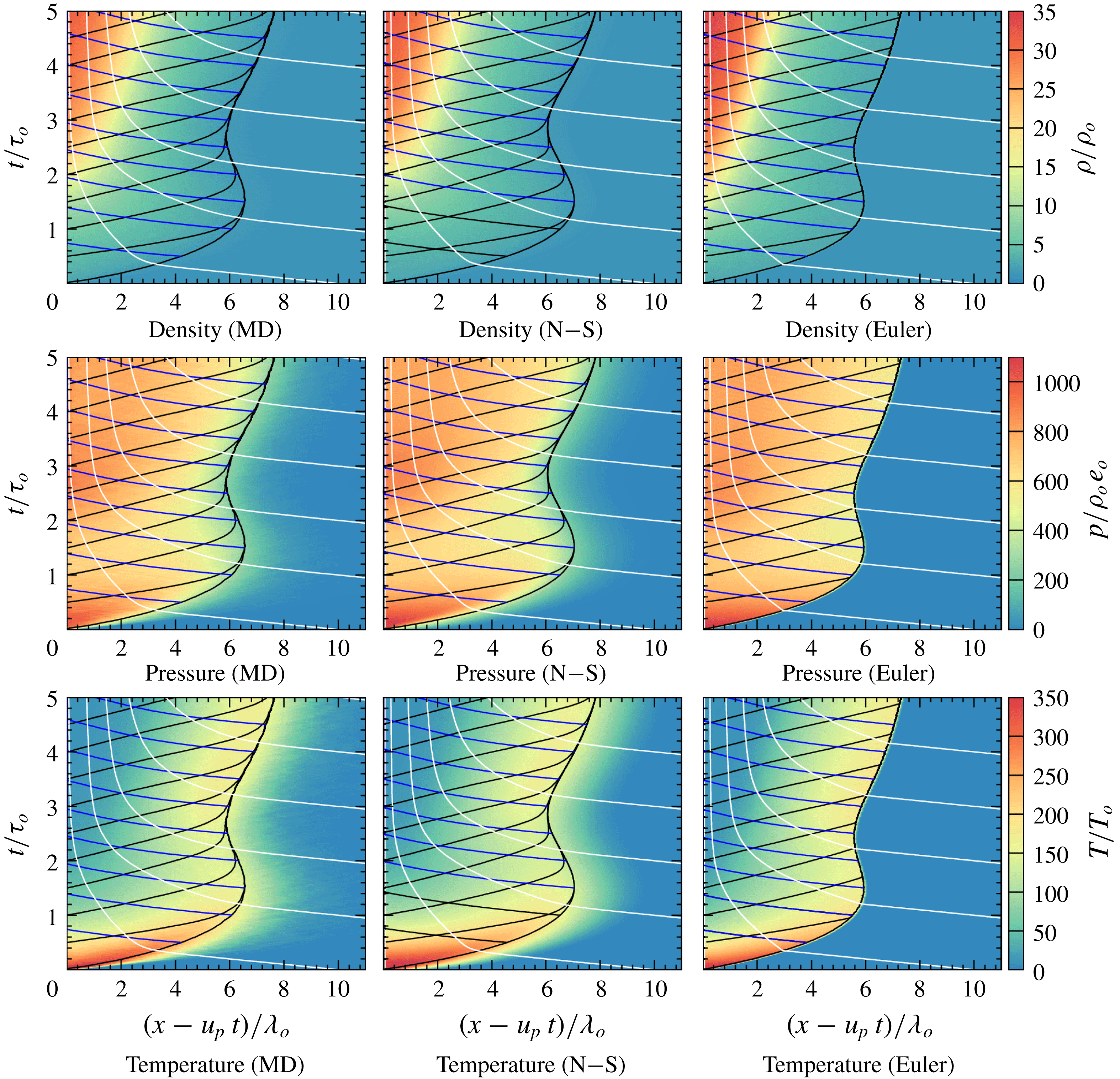
Figure 11. Evolution of density, pressure and temperature on an $x$ versus $t$ plane, in the piston frame of reference, for $u_{p}/\bar{u}_{o}=20$ , $u^{\ast }/\bar{u}_{o}=10$ , $\unicode[STIX]{x1D700}=0.95$ and $\unicode[STIX]{x1D702}_{o}=0.012$ . Also shown are select particle paths (white), forward (black) and backward (blue) running characteristics.

Figure 11 shows the evolution of density, pressure and temperature obtained from the MD and continuum models for the case shown in figure 9. The evolutions are shown with selected particle paths in white, $C^{+}$ characteristics extending from the piston in black, and $C^{-}$ characteristics from the shock front in blue. The $C^{+}$ characteristics converge along the shock front due to a sharp change in $u+c$ . All models give similar trends, although the Euler solution shows sharp jumps in density, pressure and temperature at the shock front, as expected due to the lack of diffusive terms. This differs from the MD and N–S results where the macroscopic states were smeared on the shock front. Also seen from the shock trajectory is that there is no apparent unstable behaviour once it reached the steady structure.

The evolution of the shock structure can be broken up and described in different stages based on the results given in figure 11. At the beginning of the shock development, there are large initial jumps in temperature and pressure, which gives rise to a fast shock wave. Following this initial stage, the shock decelerates rapidly, eventually pulling back towards the piston after roughly one mean free time (at $t/\unicode[STIX]{x1D70F}_{o}\approx 1.5$ ), thus recovering what is observed for purely inelastic media (Kamenetsky et al. Reference Kamenetsky, Goldshtein, Shapiro and Degani2000). The shock then accelerates and tends to the developed structure at $t/\unicode[STIX]{x1D70F}_{o}\approx 2.5$ .

To further investigate the stages of the evolution, including the reversal of the shock front to the piston, the interaction of characteristics with the evolution of temperature, density and pressure, were analysed. A Lagrangian approach was taken to explain the transient stages by tracking how properties of particle paths along the piston are communicated forward. Figure 12(a) gives the density, pressure and temperature for a particle path which originates close to the piston face, as obtained from the N–S simulation. Figure 12(b) gives a comparison between the evolution of shock front speed and the pressure along this particle path.

Figure 12. (a) Comparison of particle path properties along piston face, and (b) comparison between pressure experienced by particle path along piston face and shock front velocity, as obtained from N–S for $u_{p}/\bar{u}_{o}=20$ , $u^{\ast }/\bar{u}_{o}=10$ , $\unicode[STIX]{x1D702}_{o}=0.012$ and $\unicode[STIX]{x1D700}=0.95$ .

The first stages in the evolution can be related to the decay and pull back of the shock front. During these early stages, the initially shocked particle paths were shown to experience a strong temperature decay due to the inelastic collisions, as shown in figure 12(a). This decay in temperature leads to a drop in pressure and increase in density. The rapid decay experienced by these particle paths were communicated to the shock front via $C^{+}$ characteristics traversing through the particle paths, which caused the shock to slow down. The shock speed eventually became negative with respect to the piston at $t/\unicode[STIX]{x1D70F}_{o}\approx 1.5$ .

The next stage is attributed to a re-pressurization felt along the piston face. At $t/\unicode[STIX]{x1D70F}_{o}\approx 1.3$ , the pressure felt along the particle path stopped decreasing and began increasing, which can be attributed to the increasing density and compressibility factor playing a larger role than the decreasing temperature via the equation of state. This re-pressurization event can be seen communicating forward to the shock front, causing the shock to accelerate at $t/\unicode[STIX]{x1D70F}_{o}\approx 2.2$ . The delay between the pressure increasing at $t/\unicode[STIX]{x1D70F}_{o}\approx 1.3$ and the accelerating shock front at $t/\unicode[STIX]{x1D70F}_{o}\approx 2.2$ in figure 12(b) can be explained by the time it takes for $C^{+}$ characteristics to be communicated from the piston to the shock front.

At $t/\unicode[STIX]{x1D70F}_{o}\approx 2.8$ the pressure along the piston began decreasing, leading to a deceleration of the shock front. The dropping pressure is attributable to the temperature decay having a larger effect via the equation of state than the density change on the pressure. The pressure eventually stopped changing near $t/\unicode[STIX]{x1D70F}_{o}\approx 4.5$ , with the change in density and temperature counteracting to maintain a constant pressure. The constant pressure is attributable to the beginning of the ‘equilibrium’ region, which leads to a constant shock speed following shortly after. The steady-state structure was formed once the ‘equilibrium’ region began extending from the piston.

Figure 13. Comparison of pressure experienced by different particle paths obtained from N–S, where $\unicode[STIX]{x1D709}=x(t=0)$ , for $u_{p}/\bar{u}_{o}=20$ , $u^{\ast }/\bar{u}_{o}=10$ , $\unicode[STIX]{x1D702}_{o}=0.012$ and $\unicode[STIX]{x1D700}=0.95$ .

Particle paths that traversed the shock front at later times, as shown in figure 13, did not experience the complex re-pressurization event and had no effect on changing the structure.

5.2 Effect of $u^{\ast }$ , $\unicode[STIX]{x1D700}$ and $\unicode[STIX]{x1D702}_{o}$ on the transient relaxation

Figure 14. Evolution of pressure and characteristics as obtained from N–S for $u_{p}/u^{\ast }=0.5$  (a), 1.0 (b), 1.5 (c) and 2.0 (d) for $u^{\ast }/\bar{u}_{o}=10$ , $\unicode[STIX]{x1D702}_{o}=0.012$ and $\unicode[STIX]{x1D700}=0.95$ .

Figure 15. Comparison of pressure felt for particle paths along the piston face compared to the shock front velocity relative to the piston, as obtained from N–S for $u_{p}/\bar{u}_{o}=5$  (a), 10 (b), 15 (c) and 20 (d), $u^{\ast }/\bar{u}_{o}=10$ , $\unicode[STIX]{x1D702}_{o}=0.012$ and $\unicode[STIX]{x1D700}=0.95$ .

In § 4, it was shown that for a given piston speed or shock speed, the steady structure was uniquely described by the three non-dimensional parameters $D/u^{\ast }$ , $\unicode[STIX]{x1D700}$ and $\unicode[STIX]{x1D702}_{o}$ . Since an analytical solution for the transient development is not available, it is worthwhile assessing the influence of these parameters on the transient relaxation to a steady state.

Figure 14 shows the dependence of the magnitude of the piston speed compared with the activation threshold $u^{\ast }$ , while figure 15 shows the evolution of the shock speed and pressure at the piston face. At a low piston speed, figure 14(a) shows that the shock front monotonously decayed to a steady state and did not experience any pull back towards the piston. Analysis of the characteristics shows that the early particle paths did not experience any rapid re-pressurization, leading to the shock front velocity remaining positive with respect to the piston, as seen in figure 15(a). Although there was a small decay in shock velocity, the trend is similar to that observed for elastic media for start-up of a viscous shock wave.

With increasing piston speed, as shown in figure 14(b), there was a more rapid decay in the shock front velocity before obtaining a constant velocity. The properties of the particle path along the piston face, shown in figure 15(b), show that there was a gradual re-pressurization experienced at early times, with the drop in pressure not sufficient for the shock front velocity to slow down and pull back towards the piston before the re-pressurization was felt at the shock front.

Figure 14(c) shows the evolution for $u_{p}/u^{\ast }=1.5$ . In this case, there was a rapid decay in the shock front velocity, leading to the shock pulling back towards the piston in the N–S simulations. The properties of the particle path along the piston face are shown in figure 15(c). Results show that there was a rapid drop in pressure at early times, which was sufficient to cause the shock speed to become negative with respect to the piston before the re-pressurization was communicated forward causing the shock front to accelerate.

Finally, figure 14(d) shows the evolution for $u_{p}/u^{\ast }=2.0$ , as previously discussed. This case showed that increasing the ratio of $u_{p}/u^{\ast }$ causes a larger pressure drop to be experienced by the early particle paths. This ultimately leads to the shock front velocity becoming negative with respect to the piston before the re-pressurization was able to be communicated forward to accelerate the shock front.

The results presented in figures 14 and 15 show that the behaviour of the shock wave evolution changes with $u_{p}/u^{\ast }$ , which was shown to play an important part on the shock structure in § 4. For large values of this ratio ( $u_{p}/u^{\ast }\geqslant 2.0$ ) the behaviour computed by Kamenetsky et al. (Reference Kamenetsky, Goldshtein, Shapiro and Degani2000) is recovered. However, decreasing this ratio leads to an increased number of elastic collisions being present during the evolution, leading to a transition between this purely inelastic behaviour, and what is expected for elastic media.

Figure 16 shows the effect of $\unicode[STIX]{x1D700}$ on the evolution of the shock structure and differences between the MD and continuum models for $u_{p}/\bar{u}_{o}=20$ , $u^{\ast }/\bar{u}_{o}=10$ , $\unicode[STIX]{x1D702}_{o}=0.012$ . Results show that all values of $\unicode[STIX]{x1D700}$ gave the same behaviour of the shock front pulling back towards the piston, although the time and distance from the piston for the pull back differ. Figure 16(a) shows that for $\unicode[STIX]{x1D700}=0.80$ the front turned to the piston at $t/\unicode[STIX]{x1D70F}_{o}\approx 0.5$ , at a distance ahead of the piston of ${\sim}1.5\unicode[STIX]{x1D706}_{o}$ for Euler and ${\sim}2.6\unicode[STIX]{x1D706}_{o}$ for N–S. The behaviour of the shock front can be described by observing the pressure felt by the particle paths near the piston, which is shown in figure 17(a). The early particle paths along the piston experienced a larger and more rapid pressure drop as $\unicode[STIX]{x1D700}$ was decreased, which can simply be attributed to a larger cooling rate. The overall dynamics was similar, with the presence of a large pressure drop, followed by a re-pressurization prior to coming to some steady value. The more rapid pressure drop lead to a quicker decrease in shock front velocity for lower $\unicode[STIX]{x1D700}$ , as shown in figure 17(b). Once the transient behaviour subsided, all values of $\unicode[STIX]{x1D700}$ obtained the same shock front velocity, as expected since the states in the equilibrium region are equal.

Figure 16. Comparison of shock front position obtained from MD, N–S and Euler simulations with $u_{p}/\bar{u}_{o}=20$ , $u^{\ast }/\bar{u}_{o}=10$ , $\unicode[STIX]{x1D702}_{o}=0.012$ and varying $\unicode[STIX]{x1D700}$ .

Figure 17. Evolution of (a) pressure felt for particle paths along the piston face, and (b) velocity relative to the piston, for different values of $\unicode[STIX]{x1D700}$ , as obtained from N–S for $u_{p}/\bar{u}_{o}=20$ , $u^{\ast }/\bar{u}_{o}=10$ and $\unicode[STIX]{x1D702}_{o}=0.012$ .

The role that the initial packing factor $\unicode[STIX]{x1D702}_{o}$ has on the relaxation process is illustrated in figure 18, obtained for $u_{p}/\bar{u}_{o}=20$ , $u^{\ast }/\bar{u}_{o}=10$ and $\unicode[STIX]{x1D700}=0.95$ . Results show that the time for the shock front reversing towards the piston was unaffected by $\unicode[STIX]{x1D702}_{o}$ , with each case reversing at $t/\unicode[STIX]{x1D70F}_{o}\approx 1.5$ . However, the distance ahead of the piston where the shock reversed to the piston increased with greater values of $\unicode[STIX]{x1D702}_{o}$ , where $\unicode[STIX]{x1D702}_{o}=0.005$ extended ${\sim}6.5\unicode[STIX]{x1D706}_{o}$ ahead of the piston before reversing, while $\unicode[STIX]{x1D702}_{o}=0.025$ extended ${\sim}8\unicode[STIX]{x1D706}_{o}$ . These differences can be attributed to the longer relaxation zone length expected for larger values of $\unicode[STIX]{x1D702}_{o}$ , as shown in § 4.

Figure 18. Comparison of shock front position obtained from N–S where $\unicode[STIX]{x1D702}_{o}$ was varied, and $u_{p}/\bar{u}_{o}=20$ , $u^{\ast }/\bar{u}_{o}=10$ and $\unicode[STIX]{x1D700}=0.95$ .

5.3 Scaling of the evolution with $u^{\ast }$

Results in § 4 indicated that, for $u_{p}/u^{\ast }\geqslant 0.3$ , equal values of $u_{p}/u^{\ast }$ yielded the same shock structure once scaling was completed with $u^{\ast }$ instead of $\bar{u}_{o}$ . Considering this finding, the evolution was compared for similar values of $u_{p}/u^{\ast }$ with time scaled by $\unicode[STIX]{x1D70F}^{\ast }=\unicode[STIX]{x1D706}_{o}/u^{\ast }$ . Figure 19 shows the location of the shock front using such a time scaling for the cases where $u_{p}$ and $u^{\ast }$ were varied to satisfy $u_{p}/u^{\ast }=2$ , with $\unicode[STIX]{x1D702}_{o}=0.012$ and $\unicode[STIX]{x1D700}=0.95$ . The results show that under this scaling, the evolution of each shock structure was nearly identical. The distance and time that the reversal towards the piston occurred were equal, occurring with the shock front $7\unicode[STIX]{x1D706}_{o}$ ahead of the piston at a time of $15\unicode[STIX]{x1D70F}^{\ast }$ .

Figure 19. Comparison of shock front position obtained from N–S where $u_{p}$ and $u^{\ast }$ are varied, with $u_{p}/u^{\ast }=2$ , $\unicode[STIX]{x1D702}_{o}=0.012$ and $\unicode[STIX]{x1D700}=0.95$ .

6.1 Stability during the shock formation phase

The MD results of Sirmas & Radulescu (Reference Sirmas and Radulescu2015) showed that the shock becomes rippled during the formation stage. The continuum descriptions are now investigated to determine if they can capture this instability. The one-dimensional simulations described in the previous section were extended to two dimensions. The incoming flow field was perturbed for a short amount of time in order to investigate whether perturbations would grow or decay.

Figure 20 shows the results for inviscid continuum simulations with $u_{p}/\bar{u}_{o}=20$ , $u^{\ast }/\bar{u}_{o}=10$ , $\unicode[STIX]{x1D700}=0.95$ and $\unicode[STIX]{x1D702}_{o}=0.012$ . For this case, the density was perturbed for incoming flow during the times $t/\unicode[STIX]{x1D70F}_{o}=0$ to 1.0. A contour line was chosen arbitrarily at $\unicode[STIX]{x1D70C}/\unicode[STIX]{x1D70C}_{o}=29$ to visualize instabilities. The results show that the structure did become unstable while the incoming flow field was being perturbed. However, as the perturbations stopped, the instabilities decayed and smeared along the piston face. Similar results were also obtained using the Navier–Stokes model, although the perturbations diffused out more rapidly. The 1-D solutions described in the previous sections were recovered. This example reveals that the structure remains unstable only when the incoming flow is continuously perturbed, with perturbations unable to amplify and sustain an unstable structure.

Figure 20. Evolution of shock structure obtained from Euler simulations where incoming flow is perturbed from $t/\unicode[STIX]{x1D70F}_{o}=0$ to 1.0 for $u_{p}/\bar{u}_{o}=20$ , $u^{\ast }/\bar{u}_{o}=10$ , $\unicode[STIX]{x1D700}=0.95$ and $\unicode[STIX]{x1D702}_{o}=0.012$ . Incoming flow is perturbed in bins of $\text{d}x=\unicode[STIX]{x1D706}_{o}$ , where $\unicode[STIX]{x1D70E}=0.33\unicode[STIX]{x1D70C}_{o}$ .

The continuum models assume that matter is continuously distributed without any fluctuations. This is not a valid representation at scales comparable to the mean free path, as density fluctuations of growing magnitude are expected to play sensible roles. When the domain of disks is divided into bins of size $\text{d}x$ , the variance in number density is inversely proportional to the cell size, yielding (Bird Reference Bird1999)

(6.1) $$\begin{eqnarray}\displaystyle \unicode[STIX]{x1D70E}=\frac{\unicode[STIX]{x1D70C}_{o}\text{d}\sqrt{\unicode[STIX]{x03C0}}}{2\sqrt{\unicode[STIX]{x1D702}}\,\text{d}x}. & & \displaystyle\end{eqnarray}$$

This result is derived in appendix A. Since it is evident that there are large fluctuations in the MD simulations, these fluctuations were incorporated into the continuum description to investigate the role they may play. To account for the statistical fluctuations, perturbations were introduced into the incoming density flow field. This was simply done by separating the domain and incoming flow into bins of size $\text{d}x\times \text{d}x$ and perturbing the density with some value $\unicode[STIX]{x1D70C}^{\prime }$ , i.e. $\unicode[STIX]{x1D70C}=\unicode[STIX]{x1D70C}_{o}+\unicode[STIX]{x1D70C}^{\prime }$ . A schematic of these perturbed cells is shown in figure 21, which compares the representative cell size in MD to the perturbed bins which were introduced in the continuum model. The amplitude of the perturbations were taken randomly within the range $-2\unicode[STIX]{x1D70E}\leqslant \unicode[STIX]{x1D70C}^{\prime }\leqslant 2\unicode[STIX]{x1D70E}$ , where $\unicode[STIX]{x1D70E}$ was given from (6.1). This range was chosen for the simple stepwise distribution used here to recover the same standard deviation given in the actual distribution from MD.

Figure 21. Schematic comparing the MD and continuum domains, where continuum simulations are perturbed in bins of size $\text{d}x\times \text{d}x$ with amplitudes in agreement with statistical fluctuations observed in MD being split into bins of similar dimensions.

Figure 22. Evolution of shock morphology obtained at different times from Euler (a–d), N–S (e–h) and MD (i–l) simulations with $u_{p}/\bar{u}_{o}=20$ , $u^{\ast }/\bar{u}_{o}=10$ , $\unicode[STIX]{x1D700}=0.95$ and $\unicode[STIX]{x1D702}_{o}=0.012$ . Continuum simulations have a perturbation size of $\text{d}x=\unicode[STIX]{x1D706}_{o}$ , which corresponds to a standard deviation of $\unicode[STIX]{x1D70E}=0.33\unicode[STIX]{x1D70C}_{o}$ .

Figure 22 shows the results for the evolution of the two-dimensional structure obtained from Euler and N–S with the inclusion of these fluctuations, for the case where $u_{p}/\bar{u}_{o}=20$ , $u^{\ast }/\bar{u}_{o}=10$ , $\unicode[STIX]{x1D700}=0.95$ and $\unicode[STIX]{x1D702}_{o}=0.012$ . For comparison, the coarse grain averaged density distribution from MD is also shown. In this case, the perturbed bins in the continuum models were given a size of $\text{d}x=\unicode[STIX]{x1D706}_{o}$ , which corresponds to a standard deviation of $\unicode[STIX]{x1D70E}=0.33\unicode[STIX]{x1D70C}_{o}$ . At initial times, a noisy flow can be seen moving towards the piston face, which leads to a jump in density with the formation of the shock wave. As time progressed, density rises rapidly at the piston face, which is seen in figure 22(b), for $t/\unicode[STIX]{x1D70F}_{o}=2.71$ . Instabilities could be seen forming in the Euler simulations at this time. At later times ( $t/\unicode[STIX]{x1D70F}_{o}=5.41$ and 8.12), N–S and MD yielded instabilities with bumps forming near the piston face and extending ahead.

Figure 23 further compares the developed structure from N–S and MD, where streamlines and pattern formation were outlined. Results for N–S show that the model recovered the same formation of convective rolls in the higher density regions. These results demonstrate that the continuum models could indeed recover the same instability seen in MD if molecular fluctuations were included. Also given in figure 23 is the relaxation length scale under these parameters which was $l_{R}\approx 7.3\unicode[STIX]{x1D706}_{o}$ , as obtained in § 4. As can be seen, both MD and N–S yielded a size of these bumps that is similar in size to $l_{R}$ . To investigate if the wavelength of the patterns was locked to the domain size, a larger domain of $y/\unicode[STIX]{x1D706}_{o}=25$ was also computed, with the results from N–S recovering a similar structure to what was seen for the smaller domain (Sirmas Reference Sirmas2017). The size of the bins and the amplitude of perturbations were also varied. The results revealed that a similar wavelength of instability can still be recovered for different bin sizes, as long as the amplitudes of perturbations are in agreement with (6.1).

Figure 23. Comparison of shock morphology obtained at $t/\unicode[STIX]{x1D70F}_{o}=8.12$ for (a) N–S and (b) MD simulations, where $u_{p}/\bar{u}_{o}=20$ , $u^{\ast }/\bar{u}_{o}=10$ and $\unicode[STIX]{x1D700}=0.95$ . Also shown is the relaxation length for these conditions, where $l_{R}\approx 7.3\unicode[STIX]{x1D706}_{o}$ . N–S simulations perturbed with bins of size $\text{d}x=\unicode[STIX]{x1D706}_{o}$ .

Figure 24 shows the resulting density distribution from (a) N–S and (b) MD for $u_{p}/u^{\ast }=3.0$ , $u^{\ast }/\bar{u}_{o}=10$ , $\unicode[STIX]{x1D700}=0.95$ and $\unicode[STIX]{x1D702}_{o}=0.012$ . Under these conditions $l_{R}\approx 5.8\unicode[STIX]{x1D706}_{o}$ , which is shown in the images. Results from MD show bumps with a similar wavelength to $l_{R}$ . Results from N–S show that the structure still remained unstable, although the wavelength of instability from N–S was larger than $l_{R}$ for these parameters. Results from (a) N–S and (b) MD still show fair agreement, demonstrating that an increasing value of $u_{p}/u^{\ast }$ yields a more compact unstable structure.

Figure 24. Comparison of shock morphology obtained at $t/\unicode[STIX]{x1D70F}_{o}=5.40$ for (a) N–S and (b) MD simulations, where $u_{p}/\bar{u}_{o}=30$ , $u^{\ast }/\bar{u}_{o}=10$ , $\unicode[STIX]{x1D700}=0.95$ and $\unicode[STIX]{x1D702}_{o}=0.012$ . Also shown is the relaxation length for these conditions, where $l_{R}\approx 5.8\unicode[STIX]{x1D706}_{o}$ . N–S simulations perturbed with bins of size $\text{d}x=\unicode[STIX]{x1D706}_{o}$ .

Figure 25. Comparison of shock morphology obtained at $t/\unicode[STIX]{x1D70F}_{o}=16.24$ for (a) N–S and (b) MD simulations, where $u_{p}/\bar{u}_{o}=10$ , $u^{\ast }/\bar{u}_{o}=10$ , $\unicode[STIX]{x1D700}=0.95$ and $\unicode[STIX]{x1D702}_{o}=0.012$ . Also shown is the relaxation length for these conditions, where $l_{R}\approx 16.8\unicode[STIX]{x1D706}_{o}$ . N–S simulations perturbed with bins of size $\text{d}x=\unicode[STIX]{x1D706}_{o}$ .

Figure 25 shows the results for $u_{p}/u^{\ast }=1.0$ , $u^{\ast }/\bar{u}_{o}=10$ , $\unicode[STIX]{x1D700}=0.95$ and $\unicode[STIX]{x1D702}_{o}=0.012$ . Under these conditions, $l_{R}\approx 16.8\unicode[STIX]{x1D706}_{o}$ , as shown in the images. Unstable patterns are difficult to see in MD, although the results from N–S demonstrate that these parameters still became unstable, with convective rolls and bumps forming along the piston face. The spacing of these patterns was shown to be similar to the relaxation length.

Results from N–S are shown in figures 26(a) and 26(b) for $u_{p}/\bar{u}_{o}=7.5$ and 5.0, respectively, with $u^{\ast }/\bar{u}_{o}=10$ , $\unicode[STIX]{x1D700}=0.95$ and $\unicode[STIX]{x1D702}_{o}=0.012$ . The coarse grain averaged properties in MD are too noisy to interpret any instabilities, and are not included. For the case where $u_{p}/u^{\ast }=0.75$ in figure 26(a), convective rolls are still seen to occur along the piston face, which occur over similar lengths to the relaxation length, which is $29.5\unicode[STIX]{x1D706}_{o}$ for these parameters. However, as $u_{p}/u^{\ast }$ is decreased to 0.50 in figure 26(b), convective rolls are no longer seen along the piston face, yielding a stable structure. For this case the relaxation length is $65.5\unicode[STIX]{x1D706}_{o}$ . These results indicate a transition between the unstable and stable structures occurring at $u_{p}/u^{\ast }\approx 0.75$ for this value of $\unicode[STIX]{x1D702}_{o}$ and $\unicode[STIX]{x1D700}$ .

Figure 26. Shock morphologies obtained from N–S for (a) $u_{p}/\bar{u}_{o}=7.5$ (where $l_{R}\approx 29.5\unicode[STIX]{x1D706}_{o}$ ) and (b) $u_{p}/\bar{u}_{o}=5.0$ , where $u^{\ast }/\bar{u}_{o}=10$ , $\unicode[STIX]{x1D700}=0.95$ and $\unicode[STIX]{x1D702}_{o}=0.012$ . Simulations perturbed with bins of size $\text{d}x=\unicode[STIX]{x1D706}_{o}$ .

Figure 27 shows the structures obtained from N–S for (a) $\unicode[STIX]{x1D700}=0.90$ , and (b) $\unicode[STIX]{x1D700}=0.80$ , with $u_{p}/\bar{u}_{o}=20$ , $u^{\ast }/\bar{u}_{o}=10$ and $\unicode[STIX]{x1D702}_{o}=0.012$ . For these cases the relaxation length scales are $3.8\unicode[STIX]{x1D706}_{o}$ for $\unicode[STIX]{x1D700}=0.90$ and $2.0\unicode[STIX]{x1D706}_{o}$ for $\unicode[STIX]{x1D700}=0.80$ . Both results show the characteristic unstable bumps observed with $\unicode[STIX]{x1D700}=0.95$ , although the bumps appear larger than the relaxation length scales. These results show that the instability becomes more compact with decreasing $\unicode[STIX]{x1D700}$ , following the trend given for $l_{R}$ in § 4.

Figure 27. Developed shock structures obtained from N–S and MD simulations at $t/\unicode[STIX]{x1D70F}_{o}=8.12$ for (a)  $\unicode[STIX]{x1D700}=0.90$ and (b)  $\unicode[STIX]{x1D700}=0.80$ , where $u_{p}/\bar{u}_{o}=20$ , $u^{\ast }/\bar{u}_{o}=10$ and $\unicode[STIX]{x1D702}_{o}=0.012$ . Also shown is the relaxation length for these conditions.

The final parameter that was investigated was the initial packing factor $\unicode[STIX]{x1D702}_{o}$ . In addition to $\unicode[STIX]{x1D702}_{o}=0.012$ shown in figure 23, $\unicode[STIX]{x1D702}_{o}=0.025$ and 0.005 were investigated, with $\unicode[STIX]{x1D700}=0.95$ , $u_{p}/\bar{u}_{o}=20$ and $u^{\ast }/\bar{u}_{o}=10$ . The results for the developed structures at these conditions are showing in figure 28. In the dense case shown in figure 28(a), where $\unicode[STIX]{x1D702}_{o}=0.025$ , an unstable structure is recovered, with large bumps similar in size to the relaxation length scale ( $l_{R}\approx 9.9\unicode[STIX]{x1D706}_{o}$ ). Similarly, the dilute case of $\unicode[STIX]{x1D702}_{o}=0.005$ , shown in figure 28(b), recovered a more compact instability, comparable in size to the relaxation length ( $l_{R}\approx 5.9\unicode[STIX]{x1D706}_{o}$ ). Similar to the dependence on $u_{p}/u^{\ast }$ and $\unicode[STIX]{x1D700}$ , varying $\unicode[STIX]{x1D702}_{o}$ modified the shock structure in accordance with the relaxation length scale. These results show that the trend applies to both the dilute and dense gas regimes.

Figure 28. Developed shock structures obtained from N–S for (a) $\unicode[STIX]{x1D702}_{o}=0.025$ and (b) $\unicode[STIX]{x1D702}_{o}=0.005$ , where $\unicode[STIX]{x1D700}=0.95$ , $u_{p}/\bar{u}_{o}=20$ and $u^{\ast }/\bar{u}_{o}=10$ . Also shown is the relaxation length for these conditions.

6.2 Stability of steady-state structure

While the previous section demonstrated that instability is manifested correctly during the shock formation stage, it is worthwhile determining if the mechanism is due to the transient pressure evolution, as argued by Sirmas & Radulescu (Reference Sirmas and Radulescu2015), or an intrinsic instability of the steady shock. The stability of the steady shock structure was thus investigated by perturbing the steady-state structure derived in § 4 for a short duration and observing whether the perturbations grow or decay. This is a similar approach to how multi-dimensional instabilities in exothermic shock waves (i.e. detonations) can be investigated (see, for example, Short & Stewart (Reference Short and Stewart1998)).

Figure 29 shows a sequence of images for the resulting evolution of the inviscid steady-state structure with $D/\bar{u}_{o}=20$ , $u^{\ast }/\bar{u}_{o}=10$ , $\unicode[STIX]{x1D700}=0.95$ and $\unicode[STIX]{x1D702}_{o}=0.012$ which was perturbed between the times $t/\unicode[STIX]{x1D70F}_{o}=0$ to 0.9. Initially, instabilities formed after perturbations were introduced, as seen at $t/\unicode[STIX]{x1D70F}_{o}=0.180$ in figure 29(b), and up to $t/\unicode[STIX]{x1D70F}_{o}=7.22$ in figure 29(d). Once the perturbations stopped, the front flattened out. During this time, instabilities were pushed back into the shock structure, and did not amplify. From this sequence it can be deduced that the shock wave is stable for the inviscid description.

Figure 29. Evolution of steady-state structure in Euler simulations where incoming flow was perturbed from $t/\unicode[STIX]{x1D70F}_{o}=0-0.9$ for $D/\bar{u}_{o}=20$ , $u^{\ast }/\bar{u}_{o}=10$ , $\unicode[STIX]{x1D700}=0.95$ and $\unicode[STIX]{x1D702}_{o}=0.012$ .

Molecular noise was also implemented into the steady structure as described above. Figure 30 shows the evolution of the inviscid shock structure perturbed continuously after $t/\unicode[STIX]{x1D70F}_{o}=0$ with bins of $\text{d}x=\unicode[STIX]{x1D706}_{o}$ . Similar to the previous case, $D/\bar{u}_{o}=20$ , $u^{\ast }/\bar{u}_{o}=10$ , $\unicode[STIX]{x1D700}=0.95$ and $\unicode[STIX]{x1D702}_{o}=0.012$ . The results show that the structure began forming instabilities immediately, visible at $t/\unicode[STIX]{x1D70F}_{o}=1.80$ . As time progressed, the instabilities continued to grow and extend back in the negative $z$ direction. This agrees with what was seen for the transient case in the previous section, whereby the inviscid results remain unstable in the presence of a continuous source of fluctuations. This again highlights the failure of continuum models neglecting the molecular noise to treat the stability problem of shocks in such dissipative gases.

Figure 30. Evolution of steady-state structure in Euler simulations where incoming flow was perturbed continuously from $t/\unicode[STIX]{x1D70F}_{o}=0$ for $D/\bar{u}_{o}=20$ , $u^{\ast }/\bar{u}_{o}=10$ , $\unicode[STIX]{x1D700}=0.95$ and $\unicode[STIX]{x1D702}_{o}=0.012$ . Incoming flow was perturbed in bins of $\text{d}x=\unicode[STIX]{x1D706}_{o}$ .

The connection between the relaxation length scales and unstable patterns was also addressed using the steady-state structure. For this case, the viscous solution was considered. Although the steady-state structure was not obtained for the viscous case, the inviscid structure could be shown to form a diffusive structure once implemented into the N–S solver and given enough time to evolve. For the case given here, the diffusive structure was shown to form after $t/\unicode[STIX]{x1D70F}_{o}=2.1$ . Therefore, in order to investigate the stability of the viscous steady-state structure, perturbations were implemented after this time required for a steady viscous structure to form.

Figure 31 gives the evolving shock structure from N–S for $D/\bar{u}_{o}=20$ , $u^{\ast }/\bar{u}_{o}=10$ , $\unicode[STIX]{x1D700}=0.95$ and $\unicode[STIX]{x1D702}_{o}=0.012$ . Perturbations were initiated after $t/\unicode[STIX]{x1D70F}_{o}=2.1$ in bins of size $\text{d}x=\unicode[STIX]{x1D706}_{o}$ . The results show that instabilities did indeed form, although at a slower rate than the inviscid model. After $t/\unicode[STIX]{x1D70F}_{o}=6.50$ , shown in figure 31(e), the characteristic unstable pattern seen in the previous section was observed. In comparing the size of the bumps, in figure 31(h), it can be seen that the bumps are similar in size to the relaxation length, which for this case is approximately $7.5\unicode[STIX]{x1D706}_{o}$ .

Figure 31. Evolution of steady-state structure in N–S simulations for $D/\bar{u}_{o}=20$ , $u^{\ast }/\bar{u}_{o}=10$ , $\unicode[STIX]{x1D700}=0.95$ and $\unicode[STIX]{x1D702}_{o}=0.012$ . Incoming flow was perturbed continuously in bins of $\text{d}x=\unicode[STIX]{x1D706}_{o}$ after $t/\unicode[STIX]{x1D70F}_{o}=2.1$ , which was the time chosen in order for the diffusive structure of the steady-state structure to have formed. The relaxation length shown in later times is $l_{R}/\unicode[STIX]{x1D706}_{o}\approx 7.5$ .

6.3 Instability mechanism

Both the formation of the shock wave and the travelling wave steady solution were found to be unstable only when molecular fluctuations were introduced. The simulations reproduced well the results using molecular dynamics, in that a ripple-like instability is established with the presence of convective rolls. The wavelength of these instabilities is comparable to the relaxation length of the shock wave structure, suggesting that it is controlled by the dissipation rate. Since the instability is also present in the steady travelling wave, this rules out the transient mechanism suggested by Sirmas & Radulescu (Reference Sirmas and Radulescu2015).

Standard explanations for shock instability are related to the shock Hugoniot (Zeldovich & Raizer Reference Zeldovich and Raizer1966; Landau & Lifshitz Reference Landau and Lifshitz1987; Fickett & Davis Reference Fickett and Davis2000). Two of the common mechanisms of instability based on the equilibrium end states are the D’yakov–Kontorovich instability and the process by which the fluid undergoes phase transitions. Previously, Sirmas & Radulescu (Reference Sirmas and Radulescu2015) used their MD results to reconstruct the shock Hugoniots and concluded that these mechanisms were not responsible for the instability observed. This analysis is not repeated here, although similar conclusions can be made using the results of the continuum models, which were found to be in very good agreement with the MD results for global shock jumps.

The important finding that molecular level fluctuations are required to reproduce the ripple-like instability suggests that the mechanism for instability is not purely hydrodynamic, but requires rarefied gas effects be incorporated in the description. Indeed, the scale of the phenomenon studied is controlled by the relaxation rate. For shocks that become unstable, the relaxation characteristic time is only a few mean free times, as discussed in § 5. It is thus not surprising that non-equilibrium effects modify the global dynamics. Here it is shown that while the mean profiles are not sensitively affected by these non-equilibrium effects, as Euler and Navier–Stokes models reproduce well the global dynamics, the stability is affected by these non-equilibrium effects in a non-trivial way.

It is worthwhile investigating the relative importance of non-equilibrium effects using the scaling arguments of Bird (Reference Bird1999) comparing the characteristic length scales of the phenomenon to the mean free path. Three limiting length scales must be considered. The first is the rarefied gas limit. This limit, which identifies whether continuum models are valid or whether a microscopic approach must be used, can be formulated in terms of the Knudsen number, $Kn=\unicode[STIX]{x1D706}/L$ , which relates the length scale of interest $L$ to the mean free path of the particles. Generally, it is assumed that continuum models are invalid when (Bird Reference Bird1999)

(6.2) $$\begin{eqnarray}\displaystyle Kn<0.1-0.2. & & \displaystyle\end{eqnarray}$$

In the current problem, the relaxation length $l_{R}$ is the length scale of interest, which would require $l_{R}>5\unicode[STIX]{x1D706}_{o}-10\unicode[STIX]{x1D706}_{o}$ in order for the continuum model to remain valid. The second limit of interest is the limit that identifies whether fluctuations play an important role in the dynamics of the problem. Bird argues that fluctuations must be considered if a box constructed with sides of the given length scale yields a standard deviation of approximately 3 % (Bird Reference Bird1999). This regime is particularly important for flows close to the dense gas regime where continuum assumption still holds, for example, in microelectromechanical systems (Gad-el Hak Reference Gad-el Hak2001). In the current two-dimensional (2-D) system, by applying (B 5), the limit is found as

(6.3) $$\begin{eqnarray}\displaystyle \unicode[STIX]{x1D70E}=\frac{\unicode[STIX]{x1D6FF}}{L}\quad \rightarrow \quad L_{crit}=\frac{\unicode[STIX]{x1D6FF}}{0.03}, & & \displaystyle\end{eqnarray}$$

where $\unicode[STIX]{x1D6FF}$ is the mean molecular spacing between particles. Given this limit, length scales exceeding this value are not expected to be influenced by molecular fluctuations, while fluctuations must be considered for length scales lower than this value. The third limit is the assumption that the gas can be treated as a dilute gas. In the limit of a dilute gas, it is assumed that there are only binary collisions, which simplifies the derivations from kinetic theory. The dilute gas assumption assumes that $\unicode[STIX]{x1D6FF}\gg d$ , with the approximate limit given as (Bird Reference Bird1999)

(6.4) $$\begin{eqnarray}\displaystyle \frac{\unicode[STIX]{x1D6FF}}{d}=7. & & \displaystyle\end{eqnarray}$$

Since $\unicode[STIX]{x1D702}=\unicode[STIX]{x03C0}/4(d/\unicode[STIX]{x1D6FF})^{2}$ from (B 4), this yields a limiting packing factor of

(6.5) $$\begin{eqnarray}\displaystyle \unicode[STIX]{x1D702}_{dilute}\lesssim 0.016. & & \displaystyle\end{eqnarray}$$

The relaxation length scales $l_{R}$ which were found in § 4 were compared to these limiting length scales. Results from § 6 showed that instabilities occurred when the value of $u_{p}/u^{\ast }\geqslant 0.75$ (specifically seen for $\unicode[STIX]{x1D702}_{o}=0.012$ and $\unicode[STIX]{x1D700}=0.95$ ). Figure 32 compares the resulting length scales for $\unicode[STIX]{x1D700}=0.95$ obtained for different packing factors, and compared with the limits discussed above. The solid symbols represent the cases where $u_{p}/u^{\ast }\geqslant 0.75$ , while the empty symbols are for piston velocities below this ratio.

Figure 32. Comparison between limits in approximations with relaxation length scales obtained from simulations for different values of $u_{p}/u^{\ast }$ and $\unicode[STIX]{x1D702}_{o}$ , with $\unicode[STIX]{x1D700}=0.95$ . The solid symbols represent the cases where $u_{p}/u^{\ast }\geqslant 0.75$ , while the empty symbols are for piston velocities below this ratio.

The results show that for low values of $u_{p}/u^{\ast }$ , $l_{R}$ lies above the limits associated with the continuum limit ( $Kn<0.1$ ) and limit for fluctuations ( $\unicode[STIX]{x1D70E}<3\,\%$ ). As $u_{p}/u^{\ast }$ increases, all values of $\unicode[STIX]{x1D702}_{o}$ begin crossing these limits. The transition at $u_{p}/u^{\ast }=0.75$ approaches the limiting boundaries while running parallel to the limit associated with particle fluctuations ( $\unicode[STIX]{x1D70E}=3\,\%$ ). Large values of $u_{p}/u^{\ast }$ yielded values of $l_{R}$ below these limits, signifying that fluctuations are important to consider and that the continuum model may not be valid. While the magnitude of the relaxation length was taken with some arbitrary equilibrium state in § 4, these results nevertheless show a connection between the size of the relaxation zone, and the need to consider statistical fluctuations.

Figure 33. Comparison between limits in approximations with relaxation length scales obtained from simulations for different values of $\unicode[STIX]{x1D700}$ , with $\unicode[STIX]{x1D702}_{o}=0.012$ and $u_{p}/u^{\ast }=2.0$ .

Section 6 demonstrated that results were in fair agreement when comparing the 2-D structure obtained from the continuum and MD models for $\unicode[STIX]{x1D700}=0.95$ . However, results in § 6.1 showed that as $\unicode[STIX]{x1D700}$ was decreased, instabilities were still shown to occur, although the wavelengths of instabilities were in disagreement. This discrepancy can be explained by comparing with the limits presented above. Figure 33 shows the values of $l_{R}$ for different values of $\unicode[STIX]{x1D700}$ , with $\unicode[STIX]{x1D702}_{o}=0.012$ and $u_{p}/u^{\ast }=2.0$ , as compared to the limiting boundaries. The results demonstrate that a decreasing value of $\unicode[STIX]{x1D700}$ significantly decreased the value of $l_{R}$ , with those given for $\unicode[STIX]{x1D700}=0.90$ and 0.80 lying well below the limit of $Kn=0.1$ . These results show that fluctuations continue to be important for such small relaxation lengths, although the continuum model may not be valid, which agrees with what was observed in § 6.1. Although $\unicode[STIX]{x1D700}=0.95$ still lies below these limits, the results from both § 5 and this section show that MD and continuum agree well, which may suggest that the definition of the relaxation length may need to be modified in future work.