1. INTRODUCTION
Classic Receiver Autonomous Integrity Monitoring (RAIM) with Global Positioning System (GPS) was designed to use single frequency (GPS L1) to provide support for “en route flight, terminal area flight, non-precision approach operations” in civil aviation (e.g., Parkinson and Axelrad, Reference Parkinson and Axelrad1988; Ochieng et al., Reference Ochieng, Sauer, Walsh, Brodin, Griffin and Denney2003; Wang and Ober, Reference Wang and Ober2009). With modernised GPS/Global Navigation Satellite System (GNSS) constellations and dual frequency capability, it is expected that future GNSS will also support “precision approach operations with both lateral and vertical guidance” for flight at 200 feet (defined as LPV-200) with new integrity monitoring schemes.
A-RAIM and R-RAIM are proposed as two parallel candidates for future generation integrity monitoring architectures to test the service availability of LPV-200 for worldwide coverage with modernized GNSS and augmentation systems (GEAS, 2008). With double civilian frequencies being transmitted, the ionosphere error can be measured, and therefore removed from the error source which improves the precision. The major difference between these two architectures is in the positioning method such that only the code measurements are used in A-RAIM, and both code and time-differenced carrier phase (TDCP) measurements are used in R-RAIM to ensure higher precision without the necessity of integer ambiguity resolution. TDCP is used in other applications, such as velocity estimation with standalone GPS methods (Serrano et al., Reference Serrano, Kim and Langley2004a, Reference Serrano, Kim, Langley, Itani and Ueno2004b; van Grass and Soloviev, Reference Van Graas and Soloviev2004; Ding and Wang, Reference Ding and Wang2011). R-RAIM is further divided by the location where observations from two time epochs are combined together as the range domain R-RAIM and the position domain R-RAIM which results in different errors and projection matrices. With advantages in R-RAIM, the trade-off is more complicated errors and projection matrices, and therefore a more complicated process to transfer these errors with given risks in RAIM.
By the number of alternative hypotheses, there are two types of RAIM algorithms for both A-RAIM and R-RAIM: the Classic RAIM method with single alternative hypothesis (e.g., Lee, Reference Lee1986; Sturza, Reference Sturza1988; Parkinson and Axelrad, Reference Parkinson and Axelrad1988; Pervan, Reference Pervan1996; Ober, Reference Ober2003; Hewitson and Wang, Reference Hewitson and Wang2006, Reference Hewitson and Wang2007; Wang and Kubo, Reference Wang, Kubo, Sugimoto and Shibasaki2010), and the MHSS RAIM method (Pervan et al., Reference Pervan, Pullen and Christie1998; Blanch et al., Reference Blanch, Ene, Walter and Enge2007, Reference Blanch, Walter and Enge2008, Reference Blanch, Walter and Enge2010, Reference Blanch, Walter and Enge2012). A brief comparison of these two RAIM algorithms is provided in Blanch et al. (Reference Blanch, Walter and Enge2008).
In GEAS (2008), the Classic RAIM method is used in range domain R-RAIM, and the MHSS RAIM method is used in A-RAIM. The MHSS method for position domain R-RAIM is developed and optimized in Lee (Reference Lee2008) and Lee and McLaughlin (Reference Lee and McLaughlin2008). GEAS (2010) reported updated results with A-RAIM adopted as the major method and position domain R-RAIM only used when A-RAIM was not available. The MHSS method was applied on both architectures. Also, the optimization method developed for MHSS (Blanch et al., Reference Blanch, Walter and Enge2010) can be applied on A-RAIM. Recent studies on A-RAIM with the MHSS method can be found in Milner and Ochieng (Reference Milner and Ochieng2010), Rippl et al. (Reference Rippl, Spletter and Günther2011) and Wu et al. (Reference Wu, Wang and Jiang2013) with a validation study in Choi et al. (Reference Choi, Blanch, Walter and Enge2011a, Reference Choi, Blanch, Akos, Heng, Gao, Walter and Enge2011b).
To further validate the choice for the purpose of future generation integrity monitoring, a comparison study was conducted among different RAIM architectures and algorithms. The comparison of the range domain and position domain R-RAIM with the Classic RAIM method was conducted in Gratton et al. (Reference Gratton, Mathieu and Boris2010). With very similar precision from these two positioning methods, the difference in the integrity results is caused by different error propagation methods. Another comparison of A-RAIM and position domain R-RAIM is provided in Jiang and Wang (Reference Jiang and Wang2011) using the MHSS method, where the difference in the integrity results is concluded as caused by both the position precision and propagation of the errors. All existing studies on A-RAIM and R-RAIM are listed in Table 1.
Table 1. Existing A-RAIM and R-RAIM Mechanisms.
In the previous work, comparison was conducted under an un-unified RAIM framework. In this paper, a unified risk definition is used with differences only in the risk allocation process. A more comprehensive comparison is provided among all candidate RAIM architectures (A-RAIM, range domain R-RAIM, position domain R-RAIM) with both RAIM algorithms applied (Classic RAIM and MHSS RAIM). Besides analytical conclusions, a numerical example for LPV-200 is designed to compare A-RAIM and R-RAIM performances with and without optimization.
2. RECEIVER AUTONOMOUS INTEGRITY MONITORING
With RAIM being generalized as two steps: risk definition and risk allocation, the first step is introduced as follows. There are two types of risks defined in civil aviation: the integrity risk and the continuity risk. The integrity risk is the probability of Hazardously Misleading Information (PHMI) which is defined as any event where the position error is greater than the dynamically calculated Vertical Protection Level (VPL) without any alarm for more than the required Time to Alert (TTA) and the continuity risk is defined as the probability of any interruption in approach service (GEAS, 2008). The allocation of risks is as follows where the total PHMI P HMI is first divided into horizontal component, P HMI,h and vertical component, P HMI,v.
 $$P_{HMI} = P_{HMI,h} + P_{HMI,v} $$
The vertical PHMI is allocated onto each hypothesis as P HMI,i,
 $$P_{HMI,v} = \sum {P_{HMI,i}} $$
where i=0,1…m for multiple hypotheses and i=0, a for single hypothesis.
The vertical PHMI for each hypothesis P HMI,i is defined as,
 $$P_{HMI,i} = P\{ (\left| {\tilde x_v} \right| \gt VPL_i ) \cap (\left| {ts_i} \right| \lt T)|H_i \; \} P_{H_i} $$
where  ${\tilde x}_{v} $ is the vertical positioning error; the test statistics ts i for hypothesis H i is tested against the threshold T. The prior probability of hypothesis H i is
  $P_{H_i} $; i=0,1…m for multiple hypotheses and i=0, a for single hypothesis. The threshold is derived by the fault free alarm rate P cont,0,
 $$P_{cont,0} = P\{ \left| {ts_i} \right| \gt T|H_0 \} P_{H_0} $$
With the optimal weight, the positioning error and test statistic are known to be independent, concluded by uncorrelation (Ober, Reference Ober2003) and multivariate normal distribution. Equation (3) is expressed as,
 $$P_{HMI,i} = P\{ \tilde x_v \gt VPL_i |H_i \; \} P\{ \left| {ts_i} \right| \lt T|H_i \} P_{H_i} $$
 For the fault free case, the probability P{|ts i|<T|H0} is approximated to be 1. Since  $\tilde x_v $ is of central distribution, the VPL under H 0 is,
 $$VPL_0 = K\left( {1 - \displaystyle{{P_{HMI,0}} \over 2}} \right)\sigma _v $$
where K( ) is the inverse of the cumulative distribution function of a Gaussian distribution N∼(0,1) and σ v is the standard deviation of  $\tilde x_v $.
Since the position error is not of central distribution with the non-centrality parameter in both the position error and test statistic unknown under the faulty case, the derivation of the VPL is not straightforward. Different RAIM algorithms are developed to solve this problem.
2.1. The Classic RAIM Algorithm
In the Classic RAIM method, the solution of VPL a is dependent on the probability of missed detection (PMD) besides the defined risks above. The idea is to fix the size of the unknown bias with given fault free alarm rate and PMD as the Minimal Detectable Bias (Teunissen, Reference Teunissen2000), which is then transferred to the position domain by the slope parameter. The faulty VPL is,
 $$VPL_{c,a} = \delta \cdot \sigma _{ss,a} + K\left( {1 - \displaystyle{{P_{HMI,a}} \over {2P_{H_a}}}} \right)\sigma _v $$
where the non-centrality parameter is  $\delta = K(1 - {\textstyle{{P_{cont,0}} \over {2P_{H_0}}}}\, ) + K(1 - P_{md} )$; The slope parameter is proved to be equivalent with σ ss,i which is the standard deviation of the solution separation
  $\hat x_v - \hat x_{vi} $ with
  $\hat x_v $ as full set solution and
  $\hat x_{vi} $ as the subset solution with the ith observation removed (Blanch et al., Reference Blanch, Walter and Enge2010). Also, σ ss,a=max(σ ss,i).
The final solution is,
 $$VPL_c = max(VPL_0, VPL_{c,a} )$$
2.2. The MHSS RAIM Algorithm
It is not necessary to fix the PMD or the bias size in the MHSS method. With the solution separation used as the test statistic and bounded by the threshold, the other part of the position error is the subset position error that is bounded by the allocated integrity risk. Therefore, the calculation remains in the position domain. The faulty VPL is,
 $$VPL_{ss,i} = K\left( {1 - \displaystyle{{P_{cont,0}} \over {2P_{H_0}}}} \right)\sigma _{ss,i} + K\left( {1 - \displaystyle{{P_{HMI,i}} \over {2P_{H_i}}}} \right)\sigma _i $$
where σ i is the standard deviation of the subset solution error  $\tilde x_{vi} $.
The final result is,
 $$VPL_{ss} = max(VPL_0, max(VPL_{ss,i} ))$$
3. A-RAIM AND R-RAIM ARCHITECTURES
The architectures of A-RAIM and R-RAIM are compared with both the Classic and MHSS RAIM methods. A bias term is added to both architectures to obtain more conservative results (GEAS, 2008).
3.1. A-RAIM
The position error with A-RAIM is expressed as,
 $$\tilde x_A = (A^T Q_A^{ - 1} A)^{ - 1} A^T Q_A^{ - 1} (\epsilon _A + b_A + f_A )$$
where A∈Rm ×n is the design matrix; ϵ A∈ Rm ×1 is the random error of the code measurement used in A-RAIM with distribution N∼(0, Q A); b A=bE is the bias term with the scalar component as b and the vector component as the matrix of ones E ∈ Rm ×1; the fault vector f A is unknown.
Therefore, VPL under H 0 is,
 $$VPL_{A,0} = K\left( {1 - \displaystyle{{P_{HMI,0}} \over {2P_{H_0}}}} \right)\sigma _A + |S_A |b_{max} $$
where  $\sigma _A = \sqrt {[A^T Q_A^{ - 1} A]_{v,v}^{ - 1}} $ is the standard deviation of the vertical position error; S A=[(ATQ A1A)−1ATQ A−1]v is the projection matrix for bias (The notation [ ]v,v stands for the 3rd column and row of the matrix, and the notation [ ]v means the 3rd row of the matrix in this paper); b max=b mE is the bias vector with b m for the integrity calculation.
VPL under H a with the Classic RAIM method is,
 $$VPL_{A,a} = \delta \cdot \sigma _{A,ss,a} + K\left( {1 - \displaystyle{{P_{HMI,a}} \over {2P_{H_a}}}} \right)\sigma _A + |S_A |b_{max} $$
where σ A,ss,a=max(σ A,ss,i) and  $\sigma _{A,ss,i} = \sqrt {[(S_{A,i} - S_A )Q_A (S_{A,i} - S_A )^T ]_{v,v}} $ is the standard deviation of the vertical solution separation, S A,i=[(A iTQA,i− 1A i)−1A iTQA,i− 1]v with A i and Q A,i as the design matrix and covariance matrix with ith observation removed.
VPL under H i with the MHSS method is (GEAS, 2008; 2010),
 $${VPL_{A,i} = K\left(\! {1 - \displaystyle{{P_{cont,0}} \over {2P_{H_0}}}} \right)\sigma _{A,ss,i} \!+\! |S_{A,ss,i} |b_{nom,i} + K\left(\! {1 - \displaystyle{{P_{HMI,i}} \over {2P_{H_i}}}} \right)\sigma _{A,i} + |S_{A,i} |b_{max,i} }$$
where the projection matrices for the bias vector is S A,ss,i=S A−SA,i;  $\sigma _{A,i} = \sqrt {[A_i^T Q_{A,i}^{ - 1} A_i ]_{v,v}^{ - 1}} $ is the standard deviation of the vertical subset position error; b nom,i=b nEi and b max,i=b mEi, E i is E with ith element as zero and b n is used for calculation of accuracy.
Therefore, the final VPL for A-RAIM under the Classic and the MHSS methods are,
 $$VPL_{A,c} = max(VPL_{A,0}, VPL_{A,a} )$$
 $$VPL_{A,ss} = max(VPL_{A,0}, max(VPL_{A,i} ))$$
3.2. R-RAIM with the Range Domain Method
The measurements from two time epochs are added together before position estimation in the range domain R-RAIM method. The position error is,
 $$ \tilde x_r = (A^T Q_r^{ - 1} A)^{ - 1} A^T Q_r^{ - 1} (\epsilon _0 + \epsilon _\Delta + b_0 + f_\Delta ) $$
where ϵ 0 is the random error of the code measurement for the initial position estimation with distribution N∼(0,Q 0) and ϵ Δ is the random error of the TDCP measurement for the relative position estimation with distribution N∼(0,Q Δ); Q r=Q 0+Q Δ; b 0 is the bias vector in the code measurement; f Δ is the fault vector in the TDCP measurement. The code measurements with GIC (GNSS Integrity Channel) integrity information are used for initial position estimation at the initial time t-T to guarantee the integrity. Therefore, it is assumed that no fault exists in the initial position error. With the difference of carrier phase measurement between two epochs, the bias is eliminated in the TDCP measurement.
Therefore, VPL under H 0 is,
 $$ VPL_{R,r,0} = K\left( {1 - \displaystyle{{P_{HMI,0}} \over {2P_{H_0}}}} \right)\sigma _r + |R_0 |b_{max} $$
where  $\sigma _r = \sqrt {[(A^T Q_r^{ - 1} A)^{ - 1} ]_{v,v}} $, R 0=[(ATQ r−1A)−1ATQ r−1]v is the projection matrix for the bias vector.
VPL under H a with the Classic method is (GEAS, 2008; Gratton et al., Reference Gratton, Mathieu and Boris2010),
 $$ VPL_{R,r,a} = \delta \cdot \sigma _{r,ss,a} + K\left( {1 - \displaystyle{{P_{HMI,a}} \over {2P_{H_a}}}} \right)\sigma _r + |R_0 |b_{max} $$
where σ r,ss,a=max{σ r,ss,i},  $\sigma _{r,ss,i} = \sqrt {[(R_i - R_0 )Q_r (R_i - R_0 )^T ]_{v,v}} $ is the standard deviation of the vertical solution separation with R i=[(A iTQr,i− 1A i)−1A iTQr,i− 1]v and Q r,i is Q r with ith row and column eliminated.
VPL under H i with the MHSS method is,
 $$VPL_{R,r,i} = K\left( {1 - \displaystyle{{P_{cont,0}} \over {2P_{H_0}}}} \right)\sigma _{r,ss,i} + |R_{ss,i} |b_{nom} + K\left( {1 - \displaystyle{{P_{HMI,i}} \over {2P_{H_i}}}} \right)\sigma _{r,i} + |R_i |b_{max} $$
where R ss,i=R 0−R i and  $\sigma _{r,i} = \sqrt {[A_i^T Q_{r,i}^{ - 1} A_i ]_{v,v}^{ - 1}} $ is the standard deviation of the vertical subset position error.
Therefore, the final VPL for the range domain R-RAIM under the Classic and the MHSS methods are,
 $$VPL_{R,r,c} = max(VPL_{R,r,0}, VPL_{R,r,a} )$$
 $$VPL_{R,r,ss} = max(VPL_{R,r,0}, max(VPL_{R,r,i} ))$$
3.3. R-RAIM with the Position Domain Method
In the position domain method, two measurements from two epochs are estimated individually before being combined together. The position error at the initial time is,
 $$\tilde x_0 = (A_0^T Q_0^{ - 1} A_0 )^{ - 1} A_0^T Q_0^{ - 1} (\epsilon _0 + b_0 )$$
where A 0 is the design matrix at the initial time.
With Coasting Time (CT) as T, the relative position error between the initial time t-T and the current time t is,
 $$\eqalign{\tilde x_\Delta = & (A^T W_{_\Delta} A)^{ - 1} A^T W_{_\Delta} (\epsilon _\Delta + f_\Delta - {\rm \Delta} A\tilde x_0 ) \cr =& S_\Delta [\epsilon _{_\Delta} + f_\Delta - {\rm \Delta} AS_0 \left( {\epsilon _0 + b_0} \right)]} $$
where ΔA=A−A 0 is the geometry change during the CT. Only satellites in view in common at time epochs of t-T and t are used here; W Δ=(Q Δ+Q ΔA)−1 with Q ΔA=ΔA(A 0TQ 0−1A 0)−1ΔAT; The projection matrices are S0=[(A 0TQ −10A 0)−1A 0TQ 0−1, S Δ=(ATW ΔA)−1A TW Δ.
The position error is the sum of the errors at two epochs,
 $$\tilde x_p = \tilde x_0 + \tilde x_\Delta $$
Therefore, VPL under H 0 is,
 $$VPL_{R,p,0} = K\left( {1 - \displaystyle{{P_{HMI,0}} \over {2P_{H_0}}}} \right)\sigma _p + |P_0 |b_{max} $$
where P 0=[S 0−S ΔΔ AS 0]v is the projection matrix for the bias vector;  $\sigma _p = \sqrt {D[\tilde x_p ]_{v,v}} $,
  $D(\tilde x_p ) = (A_0^T Q_0^{ - 1} A_0 )^{ - 1} + (A^T W_\Delta A)^{ - 1} - (A_0^T Q_0^{ - 1} A_0 )^{ - 1} {\rm \Delta} A^T S_\Delta ^T - S_\Delta {\rm \Delta} A(A_0^T Q_0^{ - 1} A_0 )^{ - 1} $.
VPL under H a with the Classic method is (Gratton et al., Reference Gratton, Mathieu and Boris2010),
 $$VPL_{R,p,a} = \delta \cdot \sigma _{\,p,ss,a} + K\left( {1 - \displaystyle{{P_{HMI,a}} \over {2P_{H_a}}}} \right)\sigma _p + |P_0 |b_{max} $$
where σ p,ss,a=max{σ p,ss,i},  $\sigma _{\,p,ss,i}\! =\! \sqrt {D(\hat x_{\Delta, i}\! -\! \hat x_\Delta )_{v,v}}, D(\hat x_{\Delta, i} \!-\! \hat x_\Delta )\! =\! (S_{{\rm \Delta}, i}\! -\! S_{\rm \Delta} ) (Q_\Delta\! +\! Q_{\Delta A} )$, and S Δ,i=(ATW Δ,iA)−1ATW Δ,i, W Δ,i is W Δ with the ith row and column eliminated.
VPL under H i with the MHSS method is (Lee, Reference Lee2008; GEAS, 2010),
 $$VPL_{R,p,i} = K\left( {1 - \displaystyle{{P_{cont,0}} \over {2P_{H_0}}}} \right)\sigma _{\,p,ss,i} + |P_{{\rm \Delta}, i} |b_{nom} + K\left( {1 - \displaystyle{{P_{HMI,i}} \over {2P_{H_i}}}} \right)\sigma _{\,p,i} + |P_i |b_{max} $$
where the projection matrices are P i=(S 0−S Δ,iΔAS 0)v, P Δ,i=(S Δ,iΔAS 0−S ΔΔAS 0)v; the standard deviation is  $\sigma _{\,p,i} = \sqrt {D(\tilde x_{\Delta, i} + \tilde x_0 )_{v,v}} $ with
  $D(\tilde x_{\Delta, i} + \tilde x_0 ) = (A_0^T Q_0^{ - 1} A_0 )^{ - 1} + (A^T W_{\Delta, i} A)^{ - 1} - (A_0^T Q_0^{ - 1} A_0 )^{ - 1} \Delta A^T S_{\Delta, i}^T - S_{\Delta, i} \Delta A(A_0^T Q_0^{ - 1} A_0 )^{ - 1} $.
Therefore, the final VPL for position domain R-RAIM under the Classic and the MHSS methods are,
 $$VPL_{R,p,c} = max(VPL_{R,p,0}, VPL_{R,p,a} )$$
 $$VPL_{R,p,ss} = max(VPL_{R,p,0}, max(VPL_{R,p,i} ))$$
4. OPTMIZATION FOR THE CLASSIC AND MHSS RAIM METHODS
With the total integrity risk given, the way to allocate it onto each hypothesis is uncertain. To take advantage of this uncertainty, the allocation is optimized so that VPL derived from each hypothesis is equal. In this way, the final maximum VPL is minimized. This optimization method is used for the MHSS method (Lee, Reference Lee2008; Blanch et al., Reference Blanch, Walter and Enge2010) by applying VPL 0=VPL ss,i=VPL ss,opt on Equations (2) (6) and (9). Therefore, the optimized VPL is derived by,
 $${2P_{H_0} N\left(\! { - \displaystyle{{VPL_{ss,opt}} \over {\sigma _v}}} \right)\! +\! \mathop \sum \limits_{i = 1}^m 2P_{H_i} N\left(\! { - \displaystyle{{VPL_{ss,opt} - K\left(\!1 \!- \displaystyle{{P_{cont,0}} \over {2P_{H_0}}} \right)\sigma _{ss,i}} \over {\sigma _i}}} \right)\! =\! P_{HMI,v}} $$
The same method can be used for the Classic RAIM method with VPL 0=VPL c,a=VPL c,opt applied in Equations (2), (6) and (7). And the optimal VPL can be derived by,
 $$2P_{H_0} N\left( { - \displaystyle{{VPL_{c,opt}} \over {\sigma _v}}} \right) + 2P_{H_a} N\left( { - \displaystyle{{VPL_{c,opt} - \delta \cdot \sigma _{ss,a}} \over {\sigma _v}}} \right) = P_{HMI,v} $$
5. COMPARISON OF A-RAIM AND R-RAIM
5.1. Comparison with original Classic and MHSS Methods
Generally, the difference between A-RAIM and R-RAIM is caused by different positioning methods. With the same RAIM algorithm, the difference between these architectures in calculating the upper bound is in the error model and the error projection matrix. The differences were tested on two RAIM algorithms with different mechanisms to allocate risks onto the position error. To get explicit numerical results for LPV-200, the following numerical example was designed.
The definition of the error model for both architectures can be found in GEAS (2008, 2010). The nominal bias is 0·1 m and the maximum bias is 0·75 m. User Range Error (URE) is 0·25 m and User Range Accuracy (URA) is 0·5 m. The total integrity risk is 2×10⁻⁷ which is evenly divided into the horizontal and vertical cases. Within the vertical case, the multiple fault modes are excluded, leaving the single fault and fault free hypotheses with total integrity risk as 8·7×10−8. The integrity risk is distributed evenly onto each hypothesis. The prior probability for each single fault mode is 1×10⁻⁵. The prior probability for null hypothesis is approximated as 0. The total continuity risk is 9·2×10−6 and the probability of the fault free and single fault modes is 8×10⁻⁶. The PMD is 10−3 for the Classic method.
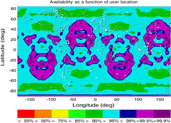
The almanac data from the standard GPS constellation with 24 satellites is used to decide the geometry at each location with 5×5 degree grid on the world map at 50 m altitudes. With the error model described above, results of VPL at each location are decided with one minute interval for A-RAIM or different CT for R-RAIM within a 24 hour time span. The availability is computed by comparing each VPL value with the Vertical Alarm Limit (VAL) to decide the final availability for each location. The percentage of over 99% availability over this time is shown worldwide. The software is based on the MATLAB Algorithm Availability Simulation Tool (MAAST) by Stanford University. Figures 1 to 6 and Table 2 are results of LPV-200 availability from different methods with VAL set at 35 m.

Figure 1. 99% Availability with A-RAIM Classic.

Figure 2. 99% Availability with Range R-RAIM Method. Classic Method.

Figure 3. 99% Availability with Position R-RAIM Classic Method.

Figure 4. 99% Availability with A-RAIM MHSS Method.

Figure 5. 99% Availability with Range R-RAIM MHSS Method.

Figure 6. 99% Availability with Position R-RAIM MHSS Method, CT=1 min.
Table 2. 99% Availability with A-RAIM and R-RAIM, VAL=35 m.

*A: A-RAIM; B1: R-RAIM\ Range Domain\ CT 1 min; C1: R-RAIM\ Position Domain\ CT 1 min.
The influence of different positioning methods on different RAIM architectures can be seen from comparing the columns A/B1/C1 in Table 2 and the influence of different RAIM algorithms from the rows of Classic and MHSS RAIM. Based on the results in Table 2, conclusions may be drawn as follows:
• R-RAIM has better integrity results compared with A-RAIM, and R-RAIM with CT one minute has better precision results compared with A-RAIM. The precision results with two R-RAIM positioning methods are very close, but the position domain method has better integrity results than the range domain one.
• The Classic method has better integrity results than the MHSS method that can be explained by a more relaxed integrity requirement for the alternative hypothesis. With same integrity risk for the faulty case and assumption of even allocation on each hypothesis, the faulty VPL with the Classic method is derived by the integrity risk m times the one used in the MHSS method.
• R-RAIM using the position domain method has a big advantage with the MHSS method compared with the other options. It is the best choice with the Classic method, but the difference with the MHSS method is more obvious.
The reason for better integrity results with the R-RAIM position domain method is as follows. It is assumed that there is only fault in the TDCP measurements and no fault in the code measurement in the initial time. With the capability to separate the delta range positioning and initial time positioning in the position domain method, the continuity risk is only allocated to the delta range position error in the position domain method instead of the total position error in the other two methods. With much better precision of the delta range position from the delta carrier phase, the standard deviation with the continuity risk allocated is much smaller, resulting in lower VPL and better availability.
The uncertainty in the R-RAIM architecture is the choice of CT, which will influence the results by the sampling rate (Jiang et al., Reference Jiang, Wang, Knight and Ding2010). If it is too small, there is not enough time for the integrity information to transfer. Three different choices of CT are tested in the following tables with both range and position domain methods.
It can be seen in Tables 3 and 4 that with the increase of the CT for the R-RAIM method, both the precision and the integrity results degraded, which is found to be caused by the loss of visible satellites and errors accumulated during the CT.
Table 3. R-RAIM Range with Different CT, VAL=35 m.
Table 4. R-RAIM Position with Different CT, VAL=35 m.
*B2: R-RAIM\ Range Domain\ CT 2 min; B3: R-RAIM\ Range Domain\ CT 3 min
*C2: R-RAIM\ Position Domain\ CT 2 min; C3: R-RAIM\ Position Domain\ CT 3 min
5.2. Comparison with Optimization
The optimization method described in Section 4 is applied on each candidate and simulation results are shown in Tables 5 and 6.
Table 5. A-RAIM and R-RAIM with Optimization, VAL=10 m.

Table 6. A-RAIM and R-RAIM with Optimization, VAL=15 m.

Most of the VPL value is less than 15 m after optimization from Table 6. Comparing the results in Tables 5 and 6 with the original results in Table 2, this optimization method is more effective on the MHSS method. The differences among different RAIM architectures and between RAIM algorithms after optimization are much smaller than the original ones.
6. CONCLUSION
With the same definition of integrity risk and continuity risk, the Classic Receiver Autonomous Integrity Monitoring (RAIM) method has better integrity results than the Multiple Hypothesis Solution Separation (MHSS) RAIM method with architectures of Advanced RAIM (A-RAIM) and Relative RAIM (R-RAIM). However, MHSS RAIM has the potential to accommodate more complicated failure modes with the multiple hypothesis structure. With the same RAIM algorithm, the R-RAIM position domain method has the best integrity results. The advantage of using this method is most obvious with the MHSS method. Coasting time for R-RAIM in this simulation is found to be better around one minute. With a longer coasting time period, the results deteriorate with lost satellites and accumulated errors. After optimization, VPL value reduces greatly with improved availability. This optimization method has a more obvious effect on the MHSS method. With better integrity results, the disadvantages of R-RAIM include the uncertainty of the coasting time and a heavier computation burden.
ACKNOWLEDGEMENTS
The first author is sponsored by the Chinese Scholarship Council for her PhD studies at the University of New South Wales, Australia.