


1. Introduction
The study of droplet evaporation on solid surfaces has a rich history in the field of transport phenomena (see e.g. Cazabat & Guena Reference Cazabat and Guena2010; Erbil Reference Erbil2012; Stauber et al. Reference Stauber, Wilson, Duffy and Sefiane2014; Brutin & Starov Reference Brutin and Starov2018; Giorgiutti-Dauphiné & Pauchard Reference Giorgiutti-Dauphiné and Pauchard2018). While the majority of research has focused on the drying of single sessile droplets, there is broad interest in understanding the evaporation of multiple drops through experiments, simulations and theory; representative studies include Schäfle et al. (Reference Schäfle, Bechinger, Rinn, David and Leiderer1999), Sokuler et al. (Reference Sokuler, Auernhammer, Liu, Bonaccurso and Butt2010), Carrier et al. (Reference Carrier, Shahidzadeh-Bonn, Zargar, Aytouna, Habibi, Eggers and Bonn2016), Shaikeea, Jyoti & Basu (Reference Shaikeea, Jyoti and Basu2016), Laghezza et al. (Reference Laghezza, Dietrich, Yeomans, Ledesma-Aguilar, Kooij, Zandvliet and Lohse2016), Castanet et al. (Reference Castanet, Perrin, Caballina and Lemoine2016), Bao et al. (Reference Bao, Spandan, Yang, Dyett, Verzicco, Lohse and Zhang2018), Hatte et al. (Reference Hatte, Pandey, Pandey, Chakraborty and Basu2019), Chong et al. (Reference Chong, Li, Ng, Verzicco and Lohse2020) and Wray, Duffy & Wilson (Reference Wray, Duffy and Wilson2020). Among the most recent of these investigations is the theoretical analysis of Wray et al. (Reference Wray, Duffy and Wilson2020). Repurposing the mathematical derivation of Fabrikant (Reference Fabrikant1985), they presented approximate expressions for the local and integrated evaporative flux from the surface of an array of thin (i.e. disk-like) droplets. The approximate total evaporation rates were then integrated in time to calculate the evolution and lifetime of the evaporating drops. The results of these calculations were subsequently compared with the experimental measurements of Khilifi et al. (Reference Khilifi, Foudhil, Fahem, Harmand and Ben2019) involving seven droplets arranged in an I-shaped configuration.
Here, we provide a straightforward and physically insightful approach to obtain the evaporation rates of multiple droplets, which is not restricted to a particular geometry. This integral theorem-based approach and its possible extensions should be broadly useful as compared with more laborious methods that have been traditionally employed to study diffusive mass transfer problems involving two or more objects.
2. Problem statement and solution
Consider an array of droplets (all the same liquid, but possibly different sizes) numbered  $n = 1 , 2 , \ldots , N$, with
  $S_n$ denoting the free surface area of the
  $n$-th droplet (see figure 1). Let
  $\phi = \left ( c - c_\infty \right ) / \left ( c_s - c_\infty \right )$ be the dimensionless vapour concentration field, where
  $c$ is the dimensional concentration field, and
  $c_s$ and
  $c_\infty$ are its values on the free surface of the droplets and far away from them, respectively. In many practical situations, the time scale for the diffusion of the vapour concentration is much smaller than the total evaporation time of the droplets. For instance, for millimetre-sized water droplets drying in still air at room conditions, the ratio of these two time scales is very small (of the order of
  $10^{-5}$). Moreover, for slowly evaporating drops under (nearly) isothermal conditions, the advective vapour transport by the Stefan and buoyancy-driven flows can be neglected. Therefore, assuming that the transport of the vapour phase is dominated by diffusion, we then have
 \begin{equation} \nabla^2 \phi = 0, \end{equation}
with the boundary conditions
 \begin{equation} \phi = 1, \quad \text{on} \ S_1, S_2, \ldots, S_N, \quad {\boldsymbol{n}} \boldsymbol{\cdot} {\boldsymbol{\nabla}} \phi = 0, \quad \text{on} \ S_s, \quad \text{and} \quad \phi \to 0 ,\quad \text{as} \ r = |{\boldsymbol{r}}| \to \infty, \end{equation}
where  $S_s$ represents the exposed surface of the substrate,
  ${\boldsymbol {r}}$ is the position vector and
  ${\boldsymbol {n}}$ is the unit normal vector directed into the vapour phase.

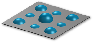
Figure 1.  $(a)$ Evaporation of four identical spherical-cap sessile droplets with contact radius
  $R$ and contact angle
  $\theta$, as an example of a multi-droplet problem described by (2.1). (b–m) Droplet arrangements considered in the validation study (see figure 2, and tables 1 and 2 of Appendix A). In each configuration, droplets with the same rate of evaporation are grouped together and labelled
  $\alpha$,
  $\beta$ or
  $\gamma$.
Our goal is to determine the rate at which the  $n$-th droplet loses mass. This quantity, represented by
  $J_n$, is obtained by integrating the flux of
  $c$ over
  $S_n$, i.e.
 \begin{equation} J_n ={-} \mathcal{D} \left( c_s - c_\infty \right) \int_{S_n} {\boldsymbol{n}} \boldsymbol{\cdot} {\boldsymbol{\nabla}} \phi \, \textrm{d}S, \end{equation}
where  $\mathcal {D}$ is the diffusion coefficient of the vapour. Conventionally, the evaporation rate is calculated after solving the boundary-value problem described by (2.1). However, for an array of droplets, as we now show, it is possible to construct an approximate expression for
  $J_n$ without directly solving for
  $\phi$.
2.1. An integral-theorem-based representation of the net fluxes
Consider the auxiliary field  ${\hat {\phi }}_n$ corresponding to the evaporation of the
  $n$-th droplet in the absence of other drops. Here
  ${\hat {\phi }}_n$ satisfies
 \begin{align}
&\nabla^2 {\hat{\phi}}_n = 0, \quad \text{with} \
{\hat{\phi}}_n = 1 ,\quad \text{on} \ S_n, \quad
{\boldsymbol{n}} \boldsymbol{\cdot} {\boldsymbol{\nabla}}
{\hat{\phi}}_n = 0, \quad \text{on} \ S_{\hat{s}} \quad \text{and}\notag\\
& {\hat{\phi}}_n \to 0, \quad
\text{as} \ r \to \infty,
\end{align}
\begin{align}
&\nabla^2 {\hat{\phi}}_n = 0, \quad \text{with} \
{\hat{\phi}}_n = 1 ,\quad \text{on} \ S_n, \quad
{\boldsymbol{n}} \boldsymbol{\cdot} {\boldsymbol{\nabla}}
{\hat{\phi}}_n = 0, \quad \text{on} \ S_{\hat{s}} \quad \text{and}\notag\\
& {\hat{\phi}}_n \to 0, \quad
\text{as} \ r \to \infty,
\end{align}
where  $S_{\hat {s}}$ denotes the non-wetted area of the substrate. Next, apply Green's second identity (see e.g. Vandadi, Jafari Kang & Masoud Reference Vandadi, Jafari Kang and Masoud2016; Masoud & Stone Reference Masoud and Stone2019) between
  $\phi$ and
  ${\hat {\phi }}$ to arrive at
 \begin{equation} \int_{S_1+S_2+\cdots+S_N+S_s+S_\infty} {\hat{\phi}} \, {\boldsymbol{n}} \boldsymbol{\cdot} {\boldsymbol{\nabla}} \phi \, \textrm{d}S = \int_{S_1+S_2+\cdots+S_N+S_s+S_\infty} \phi \, {\boldsymbol{n}} \boldsymbol{\cdot} {\boldsymbol{\nabla}} {\hat{\phi}} \, \textrm{d}S, \end{equation}
where  $S_\infty$ represents a bounding surface at infinity. Integrals over
  $S_\infty$ vanish since both
  $\phi$ and
  ${\hat {\phi }}_n$ decay sufficiently fast at large distances. Integrals over the bare substrate are also zero because
  ${\boldsymbol {n}} \boldsymbol {\cdot } {\boldsymbol {\nabla }} \phi = {\boldsymbol {n}} \boldsymbol {\cdot } {\boldsymbol {\nabla }} {\hat {\phi }}_n = 0$ on
  $S_s$. Hence, we obtain
 $$\begin{gather}
\int_{S_n} {\hat{\phi}}_n \, {\boldsymbol{n}}
\boldsymbol{\cdot} {\boldsymbol{\nabla}} \phi \,
\textrm{d}S + \sum_{\substack{m = 1 , \\ m {\!\neq} n}}^N \int_{S_m} {\hat{\phi}}_n \, {\boldsymbol{n}}
\boldsymbol{\cdot} {\boldsymbol{\nabla}} \phi \,
\textrm{d}S \nonumber\\ = \int_{S_n} \phi \,
{\boldsymbol{n}} \boldsymbol{\cdot} {\boldsymbol{\nabla}}
{\hat{\phi}}_n \, \textrm{d}S + \sum_{\substack{m = 1 , \\
m {\!\neq} n}}^N \int_{S_m} \phi \, {\boldsymbol{n}}
\boldsymbol{\cdot} {\boldsymbol{\nabla}} {\hat{\phi}}_n \,
\textrm{d}S,
\end{gather}$$
$$\begin{gather}
\int_{S_n} {\hat{\phi}}_n \, {\boldsymbol{n}}
\boldsymbol{\cdot} {\boldsymbol{\nabla}} \phi \,
\textrm{d}S + \sum_{\substack{m = 1 , \\ m {\!\neq} n}}^N \int_{S_m} {\hat{\phi}}_n \, {\boldsymbol{n}}
\boldsymbol{\cdot} {\boldsymbol{\nabla}} \phi \,
\textrm{d}S \nonumber\\ = \int_{S_n} \phi \,
{\boldsymbol{n}} \boldsymbol{\cdot} {\boldsymbol{\nabla}}
{\hat{\phi}}_n \, \textrm{d}S + \sum_{\substack{m = 1 , \\
m {\!\neq} n}}^N \int_{S_m} \phi \, {\boldsymbol{n}}
\boldsymbol{\cdot} {\boldsymbol{\nabla}} {\hat{\phi}}_n \,
\textrm{d}S,
\end{gather}$$which further simplifies to
 \begin{equation} J_n - \mathcal{D} \left( c_s - c_\infty \right) \sum_{\substack{m = 1 , \\ m {\!\neq} n}}^N \int_{S_m} {\hat{\phi}}_n \, {\boldsymbol{n}} \boldsymbol{\cdot} {\boldsymbol{\nabla}} \phi \, \textrm{d}S = {\skew4\hat{J}}_n \end{equation}
by using the boundary conditions in (2.1b) and (2.3), recalling the definitions of  $J$ and
  ${\skew4\hat{J}}$, and recognizing that
  $\int _S {\boldsymbol {n}} \boldsymbol {\cdot } {\boldsymbol {\nabla }} {\hat {\phi }}_n \, \textrm {d}S = \int _V \nabla ^2 {\hat {\phi }}_n \, \textrm {d}V = 0$, where
  $S$ is the surface enclosing the volume
  $V$ located outside of the
  $n$-th droplet. Indeed, (2.6), which is an exact relation for the total flux from any drop
  $n$ in an array of
  $N$ drops, recovers Fabrikant's formula for the net flux of a potential flow through a perforated plate with arbitrarily distributed circular holes (Fabrikant Reference Fabrikant1985), which was obtained via a series of complex transformations (see also Wray et al. Reference Wray, Duffy and Wilson2020).
2.2. An approximation scheme for solving (2.6)
To determine  $J_n$, according to (2.6), we need to approximate the surface integrals over
  $S_m$. From the method of reflections,
  $\phi$ in the neighbourhood of the
  $m$-th droplet (i.e. near
  $S_m$) can be expressed as
 \begin{equation} \phi = \phi^{(0)}_m + \sum_{i = 1}^\infty \left( \phi^{(i)}_m + \sum_{\substack{n = 1 , \\ n {\!\neq} m}}^N \phi^{(i-1)}_n \right), \end{equation}
where
 \begin{equation} \phi^{(0)}_m = \frac{J_m}{{\skew4\hat{J}}_m} \, {\hat{\phi}}_m \quad \text{and} \quad \phi^{(i)}_m = \sum_{\substack{n = 1 , \\ n {\!\neq} m}}^N \phi^{(i,n)}_m, \quad \text{for} \ i \ge 1, \end{equation}
with  $\phi ^{(i,n)}_m$ being the correction field in response to the non-uniform disturbances arising from
  $\phi ^{(i-1)}_n$ (e.g. see Kim & Karilla Reference Kim and Karilla2005; Michelin, Guérin & Lauga Reference Michelin, Guérin and Lauga2018). Note that, by definition, the reflections make no contribution to the net flux from
  $S_m$, i.e.
 \begin{equation} \int_{S_m} {\boldsymbol{n}} \boldsymbol{\cdot} {\boldsymbol{\nabla}} \phi^{(i,n)}_m \, \textrm{d}S = \int_{S_m} {\boldsymbol{n}} \boldsymbol{\cdot} {\boldsymbol{\nabla}} \phi^{(i-1)}_n \, \textrm{d}S = 0, \quad \text{for} \ n \neq m \quad \text{and} \quad i \ge 1. \end{equation}
In the same neighbourhood, we can also write  ${\hat {\phi }}_n ({\boldsymbol {r}})$ in the form of a Taylor series expansion about a judiciously chosen point
  ${\boldsymbol {r}}_m$ (located in or about droplet
  $m$) as
 \begin{equation} {\hat{\phi}}_n ({\boldsymbol{r}}) = \left.{\hat{\phi}}_n \right|_{{\boldsymbol{r}} = {\boldsymbol{r}}_m} + \left.\left( {\boldsymbol{r}} - {\boldsymbol{r}}_m \right) \boldsymbol{\cdot} {\boldsymbol{\nabla}} {\hat{\phi}}_n \right|_{{\boldsymbol{r}} = {\boldsymbol{r}}_m} + \tfrac{1}{2}\left( {\boldsymbol{r}} - {\boldsymbol{r}}_m \right) \left( {\boldsymbol{r}} - {\boldsymbol{r}}_m \right) :\left. {\boldsymbol{\nabla}} {\boldsymbol{\nabla}} {\hat{\phi}}_n \right|_{{\boldsymbol{r}} = {\boldsymbol{r}}_m} + \cdots. \end{equation}
Replacing  ${\hat {\phi }}_n$ and
  $\phi$ in the surface integral of interest with their representations from (2.8) and (2.10), we can write the exact expression
 $$\begin{align}
&\int_{S_m} {\hat{\phi}}_n \, {\boldsymbol{n}}
\boldsymbol{\cdot} {\boldsymbol{\nabla}} \phi \,
\textrm{d}S =\left. {\hat{\phi}}_n
\right|_{{\boldsymbol{r}} = {\boldsymbol{r}}_m} \int_{S_m}
{\boldsymbol{n}} \boldsymbol{\cdot} {\boldsymbol{\nabla}}
\phi^{(0)}_m \, \textrm{d}S +\left. {\hat{\phi}}_n
\right|_{{\boldsymbol{r}} = {\boldsymbol{r}}_m} \int_{S_m}
{\boldsymbol{n}} \boldsymbol{\cdot} {\boldsymbol{\nabla}}
( \phi - \phi^{(0)}_m ) \textrm{d}S \nonumber\\
&\quad + \int_{S_m} \left( \left.{\hat{\phi}}_n - {\hat{\phi}}_n
\right|_{{\boldsymbol{r}} = {\boldsymbol{r}}_m} \right)
{\boldsymbol{n}} \boldsymbol{\cdot} {\boldsymbol{\nabla}}
\phi^{(0)}_m \, \textrm{d}S + \int_{S_m} \left(
\left.{\hat{\phi}}_n - {\hat{\phi}}_n
\right|_{{\boldsymbol{r}} = {\boldsymbol{r}}_m} \right)
{\boldsymbol{n}} \boldsymbol{\cdot} {\boldsymbol{\nabla}}
\left( \phi \right)( \phi - \phi^{(0)}_m )\,\textrm{d}S.
\end{align}$$
$$\begin{align}
&\int_{S_m} {\hat{\phi}}_n \, {\boldsymbol{n}}
\boldsymbol{\cdot} {\boldsymbol{\nabla}} \phi \,
\textrm{d}S =\left. {\hat{\phi}}_n
\right|_{{\boldsymbol{r}} = {\boldsymbol{r}}_m} \int_{S_m}
{\boldsymbol{n}} \boldsymbol{\cdot} {\boldsymbol{\nabla}}
\phi^{(0)}_m \, \textrm{d}S +\left. {\hat{\phi}}_n
\right|_{{\boldsymbol{r}} = {\boldsymbol{r}}_m} \int_{S_m}
{\boldsymbol{n}} \boldsymbol{\cdot} {\boldsymbol{\nabla}}
( \phi - \phi^{(0)}_m ) \textrm{d}S \nonumber\\
&\quad + \int_{S_m} \left( \left.{\hat{\phi}}_n - {\hat{\phi}}_n
\right|_{{\boldsymbol{r}} = {\boldsymbol{r}}_m} \right)
{\boldsymbol{n}} \boldsymbol{\cdot} {\boldsymbol{\nabla}}
\phi^{(0)}_m \, \textrm{d}S + \int_{S_m} \left(
\left.{\hat{\phi}}_n - {\hat{\phi}}_n
\right|_{{\boldsymbol{r}} = {\boldsymbol{r}}_m} \right)
{\boldsymbol{n}} \boldsymbol{\cdot} {\boldsymbol{\nabla}}
\left( \phi \right)( \phi - \phi^{(0)}_m )\,\textrm{d}S.
\end{align}$$
The first integral on the right-hand side of this relation is equal to  $- J_m / \left[ \mathcal{D} \left( c_s - c_\infty \right) \right]$, while the second integral is zero (see (2.9)). The third integral is nil, too, because
 \begin{equation} \phi^{(1,n)}_m ={-} \left( \left. \phi^{(0)}_n - \phi^{(0)}_n \right|_{{\boldsymbol{r}} = {\boldsymbol{r}}_m} \right) ={-} \frac{J_n}{{\skew4\hat{J}}_n} \left( \left.{\hat{\phi}}_n - {\hat{\phi}}_n \right|_{{\boldsymbol{r}} = {\boldsymbol{r}}_m} \right) \end{equation}
on  $S_m$ and, therefore,
 \begin{equation} \int_{S_m} \left( \left.{\hat{\phi}}_n - {\hat{\phi}}_n \right|_{{\boldsymbol{r}} = {\boldsymbol{r}}_m} \right) {\boldsymbol{n}} \boldsymbol{\cdot} {\boldsymbol{\nabla}} \phi^{(0)}_m \, \textrm{d}S ={-} \frac{J_m {\skew4\hat{J}}_n}{{\skew4\hat{J}}_m J_n} \int_{S_m} {\hat{\phi}}_m \, {\boldsymbol{n}} \boldsymbol{\cdot} {\boldsymbol{\nabla}} \phi^{(1,n)}_m \, \textrm{d}S = 0, \end{equation}
where the first equality in (2.13) results from Green's second identity, followed by the use of  ${\hat {\phi }}_m = 1$ on
  $S_m$ and (2.9). In taking the above steps, it is important to recall that
  $\phi ^{(1,n)}_m$ is responsible for cancelling out spurious non-uniformities on
  $S_m$ imposed by the first reflection from droplet
  $n$, i.e. from the field
  $\phi ^{(0)}_n = (J_n / {\skew4\hat{J}}_n) \, {\hat {\phi }}_n$.
Finally, let  $\varepsilon = R / \ell$, where
  $R$ and
  $\ell$ denote, respectively, the characteristic length scale of the largest drop (if they differ in size) and the minimum centre-to-centre distance between droplet pairs. Since
  ${\hat {\phi }}$ decays, to the leading order, as
  $1 / r$, we infer that both
  ${\hat {\phi }}_n - {\hat {\phi }}_n |_{{\boldsymbol {r}} = {\boldsymbol {r}}_m}$ and
  ${\boldsymbol {\nabla }} ( \phi - \phi ^{(0)}_m )$ scale with
  $\varepsilon ^2$, which means that the fourth integral in (2.11) scales with
  $\varepsilon ^4$. Equation (2.11), therefore, reduces to
 \begin{equation} \int_{S_m} {\hat{\phi}}_n \, {\boldsymbol{n}} \boldsymbol{\cdot} {\boldsymbol{\nabla}} \phi \, \textrm{d}S ={-} \frac{ \left.{\hat{\phi}}_n \right|_{{\boldsymbol{r}} = {\boldsymbol{r}}_m} J_m}{\mathcal{D} \left( c_s - c_\infty \right)} + {O}( \varepsilon^4 ), \end{equation}
which, upon substitution in (2.6), yields
 \begin{equation} 1 \approx \frac{J_n}{{\skew4\hat{J}}_n} + \sum_{\substack{m = 1 , \\ m {\!\neq} n}}^N \left.{\hat{\phi}}_n \right|_{{\boldsymbol{r}} = {\boldsymbol{r}}_m} \, \frac{J_m}{{\skew4\hat{J}}_n}. \end{equation}
The above expression constitutes a linear system of algebraic equations for  $J_n$ that can be readily solved provided that the solution of the single-droplet problem
  ${\hat {\phi }}$ (see (2.3)) is known. Thus, we have constructed an approximate formula for the evaporation rates of an array of multiple sessile droplets, even when the array contains a mixture of drops with different sizes and contact angles. We note that (2.15) recovers (3.2) of Wray et al. (Reference Wray, Duffy and Wilson2020) (which is identical to equation (15) of Fabrikant Reference Fabrikant1985) for the special case of disk-shaped (zero-thickness) droplets with
  ${\boldsymbol {r}}_m$ located at the centre of the disks. Perhaps more interestingly, (2.15) can also be viewed as a condition that enforces
  $\phi = 1$ on
  $S_n$ during successive reflections (see e.g. Michelin et al. Reference Michelin, Guérin and Lauga2018).
2.3. On the choice of the evaluation point  ${\boldsymbol {r}}_m$

The accuracy of (2.15) beyond  ${O}( \varepsilon )$ is dependent on the choice of the location of
  ${\boldsymbol {r}}_m$. On one hand, the conventional wisdom suggests that we set the evaluation point of the Taylor series expansion to an origin about which the multipole expansion of
  ${\hat {\phi }}$ has no dipolar term. In the context of conduction heat transfer, this point is known as the ‘centre of heat’ (see e.g. Brenner Reference Brenner1963). For example, the heat centre for spherical-cap droplets is located at the centre of their contact area. However, on the other hand, we know that
  ${\hat {\phi }}$ is continuous and
  ${\boldsymbol {n}} \boldsymbol {\cdot } {\boldsymbol {\nabla }} \phi$ is an integrable function that does not change sign on
  $S_m$. As a result, the mean value theorem for definite integrals argues for selecting a spot on the free surface of the droplet as the reference point for approximating the surface integrals in (2.6). Following this argument, as a generic approach (without extra fine-tuning), we choose the point of evaluation to be the geometric centre of
  $S_m$.
3. Discussion
To evaluate the fidelity of (2.15) with our choice of  ${\boldsymbol {r}}_m$, we compare its predictions for several test cases with the results obtained from the direct numerical solution of (2.1). Specifically, the comparisons are made for the evaporation of multiple identical spherical-cap droplets that are arranged in various configurations as depicted in figure 1(b–m). There exists an analytical solution for the evaporation of a single spherical-cap droplet with contact radius
  $R$, contact angle
  $\theta$ and free surface
  $S$ (see e.g. Lebedev Reference Lebedev1965; Popov Reference Popov2005). From this solution (which was originally expressed in a boundary-fitting toroidal coordinate system), the distribution of the dimensionless vapour concentration field takes the form of
 \begin{equation} {\hat{\phi}} = 4 A \frac{R}{{\tilde{r}}} + \left( A - 4 B \right)\frac{R^3 \left( {\tilde{r}}^2 - 3 {\tilde{z}}^2 \right)}{{\tilde{r}}^5} + {O} \left[ \left( \frac{R}{{\tilde{r}}} \right)^5 \right], \end{equation}
where
 $$\begin{gather} A = \frac{1}{8 {\rm \pi}R} \int_S {\boldsymbol{n}} \boldsymbol{\cdot} {\boldsymbol{\nabla}} {\hat{\phi}} \, \textrm{d}S = \int_0^\infty \left\{ 1 + \frac{\cosh \left[ \left( 2 {\rm \pi}- \theta \right) \tau\right] }{\cosh \left( \theta \tau \right)} \right\}^{{-}1} \,\textrm{d}\tau, \end{gather}$$
 $$\begin{gather}B = \int_0^\infty \left\{ 1 + \frac{\cosh \left[ \left( 2 {\rm \pi}- \theta \right) \tau\right] }{\cosh \left( \theta \tau \right)} \right\}^{{-}1} \tau^2 \, \textrm{d}\tau, \end{gather}$$
 ${\tilde {r}} = |{\tilde {\boldsymbol {r}}}|$ and
  ${\tilde {\boldsymbol {r}}} = {\boldsymbol {r}} - {\boldsymbol {r}}_c$ with
  ${\boldsymbol {r}}_c$ being the location of the centre of the droplet's contact area. Equation (3.1) offers an excellent approximation of
  ${\hat {\phi }}$ for
  ${\tilde {r}} / R \gtrsim 2$ (touching drops), and therefore it is used to calculate
  ${\hat {\phi }}_n |_{{\boldsymbol {r}} = {\boldsymbol {r}}_m}$ in (2.15). Note that the general form of the expansion for
  ${\hat {\phi }}$ is correct for any axisymmetric droplet. Of course, the formulae for
  $A$ and
  $B$ differ from (3.2) for non-spherical-cap shapes. Furthermore, the leading-order (i.e.
  ${O}( R / {\tilde {r}} )$) term in the expansion is valid for arbitrary geometries, with
  $A$ being dependent on the specific shape.
In addition, a finite-element approach, as implemented in COMSOL Multiphysics, is employed to carry out the numerical calculations based on (2.1) and (2.1b). The outer boundary at infinity is modelled as a large hemisphere of radius  $500 R$, whose centre coincides with the centre of the droplet arrangements. Tetrahedral elements are used to mesh the computational domain such that the grid density is the highest in the vicinity of the droplets. The accuracy of the computational scheme was validated via comparison with highly accurate numerical results for the evaporation of a pair of identical disks (see table 1 of Fabrikant Reference Fabrikant1985). Specifically, we found that the relative error of our calculations for
  $J / {\skew4\hat{J}}$ is less than
  $0.3\,\%$ for all tabulated spacings ranging from
  $\ell = 2 R$ to
  $\ell = 10 R$.
We calculated the percentage difference between the predictions of (2.15) (using (3.1)) for the normalized rates of evaporation and those calculated numerically; the results are shown in figure 2. The rates are normalized by their respective values for an isolated (but otherwise the same) droplet, and their magnitudes are tabulated in tables 1 and 2 of Appendix A. The comparisons are made for two centre-to-centre droplet spacings of  $\ell = 2.5 R$ and
  $\ell = 3 R$ (see figure 1), and three contact angles
  $\theta = {\rm \pi}/ 6, {\rm \pi}/ 3, {\rm \pi}/ 2$. Note that, in each configuration, there may be one, two or three sets of droplets with distinguished evaporation rates. These sets are labelled
  $\alpha$,
  $\beta$ and
  $\gamma$ (as shown in figure 1b–m) to facilitate the presentation of the results.

Figure 2. Percentage difference between the predictions of (2.15) (using (3.1)) for the normalized rates of evaporation and the results of the numerical simulations. The rates are normalized by their respective values for isolated (but otherwise the same) droplets, and are tabulated in tables 1 and 2 of Appendix A. The errors are calculated for the spacings  $(a)$
$(a)$  $\ell = 2.5 R$ and
  $(b)$
$(b)$  $\ell = 3 R$ (see figure 1) and for the contact angles
  $\theta = {\rm \pi}/ 6, {\rm \pi}/ 3, {\rm \pi}/ 2$. In each configuration, droplets with distinguished evaporation rates are labelled
  $\alpha$,
  $\beta$ and
  $\gamma$, as shown in figures 1(b–m).
Table 1. Normalized evaporation rates of multiple identical spherical-cap droplets (with contact radius  $R$ and contact angle
  $\theta$) arranged in various configurations as shown in figure 1(b–m) of the main text. The rates are normalized by their respective values for a single (but otherwise the same) droplet. The results are reported for the spacing
  $\ell = 2.5 R$ and contact angles
  $\theta = {\rm \pi}/ 6, {\rm \pi}/ 3, {\rm \pi}/ 2$.

Table 2. Normalized evaporation rates of multiple identical spherical-cap droplets (with contact radius  $R$ and contact angle
  $\theta$) arranged in various configurations as shown in figures 1(b–m) of the main text. The rates are normalized by their respective values for a single (but otherwise the same) droplet. The results are reported for the spacing
  $\ell = 3 R$ and contact angles
  $\theta = {\rm \pi}/ 6, {\rm \pi}/ 3, {\rm \pi}/ 2$.

Inspecting the results, we find that the approximation error of (2.15) is only a few per cent or less for most cases. It appears, however, that our formulation underestimates the rate of evaporation for high-contact angle droplets that are surrounded by their neighbours (see the red triangles of configurations g, j, l and m). However, even in these cases, the maximum error is roughly  $25\,\%$ for
  $\ell = 2.5 R$ (red triangle of configuration m in figure 2a), which sharply declines to approximately
  $10\,\%$ as the spacing increases to
  $\ell = 3 R$ (red triangle of configuration m in figure 2b). We also checked that had we set
  ${\boldsymbol {r}}_m$ to the contact area centre of the droplets (i.e. their centre of heat), the corresponding errors would have been much larger, nearly
  $40\,\%$ and
  $20\,\%$ errors, respectively. The relatively higher prediction errors are partly due to stronger shielding effects in the aforementioned configurations, which significantly decrease the evaporation rate of the
  $\alpha$-type droplets. To put this into perspective, the evaporation rate for the middle droplet in configuration m when its contact angle is
  $\theta = {\rm \pi}/ 2$ is reduced to approximately
  $15\,\%$ of the rate at which the same droplet evaporates in isolation. Overall, the results of figure 2 demonstrate the high fidelity of the evaporation rates predicted by (2.15). We reiterate that the predictions here, for a wide range of configurations, are obtained using only the solution of the single-droplet problem and solving a linear system of algebraic equations (see (2.15) and (3.1)).
In conclusion, we highlight that the implications of our findings go beyond the evaporation of sessile droplets and extend to a large class of diffusive mass transfer problems that also includes, among other problems, the dissolution of micro and nano bubbles (see e.g. Dollet & Lohse Reference Dollet and Lohse2016; Michelin et al. Reference Michelin, Guérin and Lauga2018; Zhu et al. Reference Zhu, Verzicco, Zhang and Lohse2018). Additional areas of physics that benefit from our solution strategy for the Laplace equation are potential flow, conduction heat transfer, electrostatics, etc. Moreover, we note that our derivations can be further generalized, often in a fairly straightforward fashion, to include, for example, (i) pendent drops of unequal size, (ii) transient effects, (iii) additional linear terms in the governing equation (e.g. solving for the Helmholtz rather than the Laplace equation) and (iv) Neumann or mixed (Robin) boundary conditions on  $S_n$.
Acknowledgements
We thank B. Rallabandi of University of California, Riverside, for helpful conversations.
Funding
H.A.S. thanks the National Science Foundation for support via grant CBET-2116184.
Declaration of interests
The authors report no conflict of interest.
Appendix A. Tabulated evaporation rates
The evaporation rates corresponding to figures 2(a) and 2(b) are presented in tables 1 and 2, respectively. The rates are given in a normalized form, i.e. they are divided by their respective values for a single (but otherwise the same) droplet. We note that the evaporation rate of an isolated sessile droplet can be calculated from (3.2a), and the specific values for drops with contact angles  $\theta = {\rm \pi}/ 6, {\rm \pi}/ 3, {\rm \pi}/ 2$ are, respectively,
 \begin{equation} {\skew4\hat{J}}_{{\rm \pi} / 6} = 4.416, \quad {\skew4\hat{J}}_{{\rm \pi} / 3} = 5.086 \quad \text{and} \quad {\skew4\hat{J}}_{{\rm \pi} / 2} = 2 {\rm \pi}, \end{equation}
where  ${\skew4\hat{J}}$ is non-dimensionalized by
  $\mathcal {D} R \left ( c_s - c_\infty \right )$.


