


1. Introduction
The problem of heat transfer in flows between two differentially rotating circular cylinders has been the subject of intense studies for a long time because of their importance in many industrial applications (Snyder & Karlsson Reference Snyder and Karlsson1964; Kreith Reference Kreith1968; Sorour & Coney Reference Sorour and Coney1979; Ball & Farouk Reference Ball and Farouk1989; Ball, Farouk & Dixit Reference Ball, Farouk and Dixit1989; Lee & Minkowycz Reference Lee and Minkowycz1989; Ali & Weidman Reference Ali and Weidman1990; McFadden et al. Reference McFadden, Coriell, Murray, Glicksman and Selleck1990; Kedia, Hunt & Colonius Reference Kedia, Hunt and Colonius1998; Mutabazi & Bahloul Reference Mutabazi and Bahloul2002; Fénot et al. Reference Fénot, Bertin, Dorignac and Lalizel2011). One may cite the cooling of electrical motor shafts and turbine rotors (Kreith Reference Kreith1968; Lee & Minkowycz Reference Lee and Minkowycz1989; Fénot et al. Reference Fénot, Bertin, Dorignac and Lalizel2011) or the thermal stresses of the shaft and cover of boiling water reactor pumps (Kedia et al. Reference Kedia, Hunt and Colonius1998) among many others. Annular flows between two differentially rotating cylinders with a radial temperature gradient has also been used as a model of geophysical and astrophysical systems, where both rotation and temperature gradients are the main ingredients of the flows involved (Lopez, Marques & Avila Reference Lopez, Marques and Avila2013).
We investigate the stability of the flow in a differentially rotating vertical cylindrical annulus subject to a radial temperature gradient. A weak temperature gradient induces a large convective cell with ascending flow near the hot surface and descending flow near the cold one. This flow is superimposed onto the azimuthal flow induced by rotation. The base flow, then, has two velocity components: the azimuthal velocity due to rotation of the inner cylinder, and the axial component due to the temperature gradient. The investigation of the stability of this two-velocity component flow is therefore more complicated than the circular Couette flow (CCF) or the convective flow in an annulus without rotation. The effect of a thermal gradient on the CCF in a vertical cylindrical annulus has been investigated in few studies since the experimental work of Snyder & Karlsson (Reference Snyder and Karlsson1964) in an annulus with large aspect ratio and very large radius ratio. Linear stability analysis has been performed by Chen & Kuo (Reference Chen and Kuo1990) for axisymmetric perturbations and by Ali & Weidman (Reference Ali and Weidman1990) for non-axisymmetric perturbations. It has been revisited recently by Yoshikawa, Nagata & Mutabazi (Reference Yoshikawa, Nagata and Mutabazi2013), who included an energetic analysis and the effect of centrifugal buoyancy. Lopez et al. (Reference Lopez, Marques and Avila2013) made a critical analysis of the Boussinesq approximation and investigated the effect of the centrifugal buoyancy in rapidly rotating flows and its role in geophysical and astrophysical systems. A weakly nonlinear analysis of this flow has been investigated by Auer, Busse & Gangler (Reference Auer, Busse and Gangler1996) in the small-gap approximation.
Numerical simulations of the air flow in the circular Couette system with a radial temperature gradient have been realized by Ball & Farouk (Reference Ball and Farouk1989) and Kuo & Ball (Reference Kuo and Ball1997) using a hybrid Chebyshev collocation–Fourier spectral method, i.e. the flow field was represented by a Fourier series expansion in the periodic azimuthal direction and by Chebyshev polynomial expansions in the radial and axial directions. These authors neglected the centrifugal buoyancy term. Kedia et al. (Reference Kedia, Hunt and Colonius1998) solved the flow equations taking into account the centrifugal buoyancy term but using periodic conditions; they used Fourier series in the azimuthal and axial directions and a Chebyshev polynomial expansion in the radial direction. They investigated the variation of heat transfer coefficient with temperature difference for air flow in Couette–Taylor systems with three gap widths. They pointed out the sensitivity of the heat transfer to the wavenumber, its asymmetry with the sign of the temperature gradient, and the existence of stationary axisymmetric vortices for small values of temperature difference, for which the heat transfer is weakened.
The present study aims to perform numerical simulations of the thermal effects induced by a radial temperature gradient in a large-aspect-ratio Couette–Taylor system using the no-slip conditions at the top and bottom endplates instead of periodic boundary conditions. The flow system corresponds to the experimental system of Lepiller et al. (Reference Lepiller, Yoon, Prigent, Yang and Mutabazi2006, Reference Lepiller, Goharzadeh, Prigent and Mutabazi2008). The choice of such a large aspect ratio is motivated by the avoidance of the difficulties related to small aspect ratio, such as vertical temperature gradient due to thermal boundary layers. In fact, the length of the annulus must be chosen in such a way as to ensure that the base state is a conduction regime for weak values of the temperature difference, which depends on the thermal properties of the working fluids (de Vahl Davis & Thomas Reference de Vahl Davis and Thomas1969). Moreover, Kuo & Ball (Reference Kuo and Ball1997) have pointed out that the small aspect ratio used in their numerical simulations may be one reason for discrepancies with their experimental results. The influence of the endplates on both the velocity and temperature fields has been thoroughly characterized. The large aspect ratio allows the discrimination of these endplate effects from the mechanisms driving the flow instabilities. We give a detailed description of the spatio-temporal properties of flow patterns. The torque on the inner cylinder, the radial heat transfer coefficient and the vertical heat flux induced by thermo-convective structures have been computed for a fixed rotation rate and an increase of the temperature difference imposed on cylindrical surfaces.
The paper is organized as follows. In § 2, we present the flow equations, the derivation of the quantities to be computed and the numerical procedure. Results are given in § 3 and discussed in § 4. The last section contains the conclusion.
2. Problem formulation
2.1. Flow equations
We consider the flow of a Newtonian fluid of kinematic viscosity
 ${\it\nu}$
, thermal diffusivity
${\it\nu}$
, thermal diffusivity
 ${\it\kappa}$
and thermal expansion
${\it\kappa}$
and thermal expansion
 ${\it\alpha}$
in an annulus between two coaxial long cylinders, with the inner one rotating at the angular speed
${\it\alpha}$
in an annulus between two coaxial long cylinders, with the inner one rotating at the angular speed
 ${\it\Omega}$
and the outer one fixed (figure 1
a). The two cylinders, of height
${\it\Omega}$
and the outer one fixed (figure 1
a). The two cylinders, of height
 $L$
and radii
$L$
and radii
 $a$
and
$a$
and
 $b=a+d$
, are kept at different temperatures
$b=a+d$
, are kept at different temperatures
 $T_{1}$
and
$T_{1}$
and
 $T_{2}$
, thus creating a temperature gradient acting on the fluid in the annulus. The temperature difference
$T_{2}$
, thus creating a temperature gradient acting on the fluid in the annulus. The temperature difference
 ${\rm\Delta}T=T_{1}-T_{2}$
is assumed to be small, so that the Boussinesq approximation is used, allowing the fluid density
${\rm\Delta}T=T_{1}-T_{2}$
is assumed to be small, so that the Boussinesq approximation is used, allowing the fluid density
 ${\it\rho}$
to vary linearly with the temperature (i.e.
${\it\rho}$
to vary linearly with the temperature (i.e.
 ${\it\rho}(T)\approx {\it\rho}_{0}(1-{\it\alpha}T)$
with
${\it\rho}(T)\approx {\it\rho}_{0}(1-{\it\alpha}T)$
with
 ${\it\rho}_{0}={\it\rho}(T_{0})$
) only in the Archimedean and centrifugal buoyancy terms (Kedia et al.
Reference Kedia, Hunt and Colonius1998; Mutabazi & Bahloul Reference Mutabazi and Bahloul2002; Lopez et al.
Reference Lopez, Marques and Avila2013). Here
${\it\rho}_{0}={\it\rho}(T_{0})$
) only in the Archimedean and centrifugal buoyancy terms (Kedia et al.
Reference Kedia, Hunt and Colonius1998; Mutabazi & Bahloul Reference Mutabazi and Bahloul2002; Lopez et al.
Reference Lopez, Marques and Avila2013). Here
 $T$
denotes the difference between the fluid temperature and a reference temperature
$T$
denotes the difference between the fluid temperature and a reference temperature
 $T_{0}$
.
$T_{0}$
.

Figure 1. (a) Schematic of flow geometry, (b) cylinder cross-section and (c) a portion of a meridional section.
The resulting flow equations are (we have used the ‘traditional’ Boussinesq approximation according to Lopez et al. (Reference Lopez, Marques and Avila2013)):
 $$\begin{eqnarray}\left.\begin{array}{@{}c@{}}\boldsymbol{{\rm\nabla}}\boldsymbol{\cdot }\boldsymbol{u}=0,\\ \displaystyle \frac{\partial \boldsymbol{u}}{\partial t}+(\boldsymbol{u}\boldsymbol{\cdot }\boldsymbol{{\rm\nabla}})\boldsymbol{u}=-\boldsymbol{{\rm\nabla}}{\rm\pi}+{\it\nu}{\rm\nabla}^{2}\boldsymbol{u}-{\it\alpha}T\boldsymbol{G},\\ \displaystyle \frac{\partial T}{\partial t}+(\boldsymbol{u}\boldsymbol{\cdot }\boldsymbol{{\rm\nabla}})T={\it\kappa}{\rm\nabla}^{2}T,\end{array}\right\}\end{eqnarray}$$
where the reduced pressure
 ${\rm\pi}$
is given by
${\rm\pi}$
is given by
 ${\it\rho}_{0}{\rm\pi}=p+gz$
. We have introduced the effective gravity
${\it\rho}_{0}{\rm\pi}=p+gz$
. We have introduced the effective gravity
 $\boldsymbol{G}=\boldsymbol{g}+\boldsymbol{g}_{c}$
, with
$\boldsymbol{G}=\boldsymbol{g}+\boldsymbol{g}_{c}$
, with
 $\boldsymbol{g}$
the gravitational acceleration and
$\boldsymbol{g}$
the gravitational acceleration and
 $\boldsymbol{g}_{c}=(u_{{\it\varphi}}^{2}/r)\boldsymbol{e}_{r}$
the centrifugal acceleration. The nonlinear term
$\boldsymbol{g}_{c}=(u_{{\it\varphi}}^{2}/r)\boldsymbol{e}_{r}$
the centrifugal acceleration. The nonlinear term
 $(\boldsymbol{u}\boldsymbol{\cdot }\boldsymbol{{\rm\nabla}})\boldsymbol{u}$
contains, when written in cylindrical coordinates, the centrifugal and Coriolis accelerations. From the system of equations (2.1), one can derive the equations for the vorticity
$(\boldsymbol{u}\boldsymbol{\cdot }\boldsymbol{{\rm\nabla}})\boldsymbol{u}$
contains, when written in cylindrical coordinates, the centrifugal and Coriolis accelerations. From the system of equations (2.1), one can derive the equations for the vorticity
 ${\bf\omega}=\boldsymbol{{\rm\nabla}}\times \boldsymbol{u}$
,
${\bf\omega}=\boldsymbol{{\rm\nabla}}\times \boldsymbol{u}$
,
 $$\begin{eqnarray}\frac{\partial {\bf\omega}}{\partial t}+(\boldsymbol{u}\boldsymbol{\cdot }\boldsymbol{{\rm\nabla}}){\bf\omega}=({\bf\omega}\boldsymbol{\cdot }\boldsymbol{{\rm\nabla}})\boldsymbol{u}+{\it\nu}{\rm\nabla}^{2}{\bf\omega}-{\it\alpha}\boldsymbol{{\rm\nabla}}T\times \bar{\boldsymbol{G}},\end{eqnarray}$$
and for the reduced pressure
 ${\rm\pi}$
 $$\begin{eqnarray}{\rm\nabla}^{2}{\rm\pi}={\it\omega}^{2}-{\it\sigma}^{2}-{\it\alpha}\boldsymbol{{\rm\nabla}}T\boldsymbol{\cdot }\boldsymbol{G}\quad \text{with }{\it\omega}^{2}={\bf\omega}\boldsymbol{\cdot }{\bf\omega},~{\it\sigma}^{2}\equiv \boldsymbol{u}\boldsymbol{\cdot }(\boldsymbol{{\rm\nabla}}\times {\bf\omega}).\end{eqnarray}$$
The temperature gradient acts as a source of vorticity and it modifies the pressure distribution in the flow. Lopez et al. (Reference Lopez, Marques and Avila2013) have included the density variation in all the nonlinear terms as they were investigating high rotation regimes.
We have chosen the gap width
 $d$
as the scale for lengths,
$d$
as the scale for lengths,
 ${\it\Omega}a$
for velocity,
${\it\Omega}a$
for velocity,
 $d/a{\it\Omega}$
for time,
$d/a{\it\Omega}$
for time,
 ${\it\rho}({\it\Omega}a)^{2}$
for pressure and
${\it\rho}({\it\Omega}a)^{2}$
for pressure and
 ${\rm\Delta}T$
for temperature. The geometric flow parameters are the radius ratio
${\rm\Delta}T$
for temperature. The geometric flow parameters are the radius ratio
 ${\it\eta}=a/b$
and the aspect ratio
${\it\eta}=a/b$
and the aspect ratio
 ${\it\Gamma}=L/d$
. The present problem contains different time scales: the viscous diffusion time scale
${\it\Gamma}=L/d$
. The present problem contains different time scales: the viscous diffusion time scale
 ${\it\tau}_{{\it\nu}}=d^{2}/{\it\nu}$
, the thermal diffusion time scale
${\it\tau}_{{\it\nu}}=d^{2}/{\it\nu}$
, the thermal diffusion time scale
 ${\it\tau}_{{\it\kappa}}=d^{2}/{\it\kappa}$
, the centrifugal time scale
${\it\tau}_{{\it\kappa}}=d^{2}/{\it\kappa}$
, the centrifugal time scale
 ${\it\tau}_{c}=\sqrt{d/{\it\Omega}^{2}a}$
and the Archimedean time scale
${\it\tau}_{c}=\sqrt{d/{\it\Omega}^{2}a}$
and the Archimedean time scale
 ${\it\tau}_{A}=\sqrt{d/({\it\alpha}{\rm\Delta}Tg)}$
, where
${\it\tau}_{A}=\sqrt{d/({\it\alpha}{\rm\Delta}Tg)}$
, where
 ${\rm\Delta}T=T_{1}-T_{2}$
is the temperature difference between the cylinder surfaces. The ratio between these time scales determines the physical flow control parameters: the Taylor number
${\rm\Delta}T=T_{1}-T_{2}$
is the temperature difference between the cylinder surfaces. The ratio between these time scales determines the physical flow control parameters: the Taylor number
 $\mathit{Ta}={\it\tau}_{{\it\nu}}/{\it\tau}_{c}=\mathit{Re}\sqrt{d/a}$
, where the Reynolds number
$\mathit{Ta}={\it\tau}_{{\it\nu}}/{\it\tau}_{c}=\mathit{Re}\sqrt{d/a}$
, where the Reynolds number
 $\mathit{Re}={\it\Omega}ad/{\it\nu}$
; the Grashof number
$\mathit{Re}={\it\Omega}ad/{\it\nu}$
; the Grashof number
 $\mathit{Gr}=({\it\tau}_{{\it\nu}}/{\it\tau}_{A})^{2}={\it\alpha}{\rm\Delta}Tgd^{3}/{\it\nu}^{2}$
; and the Prandtl number
$\mathit{Gr}=({\it\tau}_{{\it\nu}}/{\it\tau}_{A})^{2}={\it\alpha}{\rm\Delta}Tgd^{3}/{\it\nu}^{2}$
; and the Prandtl number
 $\mathit{Pr}={\it\tau}_{{\it\kappa}}/{\it\tau}_{{\it\nu}}={\it\nu}/{\it\kappa}$
, which is a fluid property and depends only on the temperature. The Galileo number
$\mathit{Pr}={\it\tau}_{{\it\kappa}}/{\it\tau}_{{\it\nu}}={\it\nu}/{\it\kappa}$
, which is a fluid property and depends only on the temperature. The Galileo number
 $\mathit{Ga}=gd^{3}/{\it\nu}^{2}$
is characteristic of the flow system, i.e. it takes a fixed value for a given flow system. The Grashof number may be seen as the thermal Reynolds number
$\mathit{Ga}=gd^{3}/{\it\nu}^{2}$
is characteristic of the flow system, i.e. it takes a fixed value for a given flow system. The Grashof number may be seen as the thermal Reynolds number
 $\mathit{Gr}=W_{th}d/{\it\nu}$
, where
$\mathit{Gr}=W_{th}d/{\it\nu}$
, where
 $W_{th}={\it\alpha}{\rm\Delta}Tgd^{2}/{\it\nu}$
is the thermal characteristic velocity. In the rest of the paper, all the quantities are dimensionless (except in figure 1(a) where the flow geometry is illustrated with the physical dimensions). In cylindrical coordinates (
$W_{th}={\it\alpha}{\rm\Delta}Tgd^{2}/{\it\nu}$
is the thermal characteristic velocity. In the rest of the paper, all the quantities are dimensionless (except in figure 1(a) where the flow geometry is illustrated with the physical dimensions). In cylindrical coordinates (
 $r,{\it\varphi},z$
), the equations (2.1) read:
$r,{\it\varphi},z$
), the equations (2.1) read:
 $$\begin{eqnarray}\displaystyle & \displaystyle \frac{1}{r}\frac{\partial }{\partial r}(ru_{r})+\frac{1}{r}\frac{\partial u_{{\it\varphi}}}{\partial {\it\varphi}}+\frac{\partial u_{z}}{\partial z}=0, & \displaystyle\end{eqnarray}$$
 $$\begin{eqnarray}\displaystyle & \displaystyle \frac{\partial u_{r}}{\partial t}+(\boldsymbol{u}\boldsymbol{\cdot }\boldsymbol{{\rm\nabla}})u_{r}-\left[1-\frac{\mathit{Gr}}{\mathit{Ga}}T\right]\frac{u_{{\it\varphi}}^{2}}{r}=-\frac{\partial P}{\partial r}+\frac{1}{\mathit{Re}}\left[\left({\rm\nabla}^{2}-\frac{1}{r^{2}}\right)u_{r}-\frac{2}{r^{2}}\frac{\partial u_{{\it\varphi}}}{\partial {\it\varphi}}\right], & \displaystyle\end{eqnarray}$$
 $$\begin{eqnarray}\displaystyle & \displaystyle \frac{\partial u_{{\it\varphi}}}{\partial t}+(\boldsymbol{u}\boldsymbol{\cdot }\boldsymbol{{\rm\nabla}})u_{{\it\varphi}}+\frac{u_{r}u_{{\it\varphi}}}{r}=-\frac{\partial p}{r\partial {\it\varphi}}+\frac{1}{\mathit{Re}}\left[\left({\rm\nabla}^{2}-\frac{1}{r^{2}}\right)u_{{\it\varphi}}+\frac{2}{r^{2}}\frac{\partial u_{r}}{\partial {\it\varphi}}\right], & \displaystyle\end{eqnarray}$$
 $$\begin{eqnarray}\displaystyle & \displaystyle \frac{\partial u_{z}}{\partial t}+(\boldsymbol{u}\boldsymbol{\cdot }\boldsymbol{{\rm\nabla}})u_{z}=-\frac{\partial P}{\partial z}+\frac{1}{\mathit{Re}}{\rm\nabla}^{2}u_{z}+\frac{\mathit{Gr}}{\mathit{Re}^{2}}T, & \displaystyle\end{eqnarray}$$
 $$\begin{eqnarray}\displaystyle & \displaystyle \frac{\partial T}{\partial t}+(\boldsymbol{u}\boldsymbol{\cdot }\boldsymbol{{\rm\nabla}})T=\frac{1}{\mathit{Pe}}{\rm\nabla}^{2}T, & \displaystyle\end{eqnarray}$$
 $u_{r}$
,
$u_{r}$
,
 $u_{{\it\varphi}}$
and
$u_{{\it\varphi}}$
and
 $u_{z}$
denote the radial, azimuthal and axial velocity components, respectively,
$u_{z}$
denote the radial, azimuthal and axial velocity components, respectively,  $$\begin{eqnarray}\boldsymbol{u}\boldsymbol{\cdot }\boldsymbol{{\rm\nabla}}\equiv u_{r}\frac{\partial }{\partial r}+\frac{u_{{\it\varphi}}}{r}\frac{\partial }{\partial {\it\varphi}}+u_{z}\frac{\partial }{\partial z},\quad {\rm\nabla}^{2}\equiv \frac{1}{r}\frac{\partial }{\partial r}\left(r\frac{\partial }{\partial r}\right)+\frac{1}{r^{2}}\frac{\partial ^{2}}{\partial {\it\varphi}^{2}}+\frac{\partial ^{2}}{\partial z^{2}},\end{eqnarray}$$
and
 $\mathit{Pe}$
(
$\mathit{Pe}$
(
 $=\!\mathit{RePr}$
) is the Péclet number. The significance of the centrifugal buoyancy term in (2.4b
) is determined by the ratio
$=\!\mathit{RePr}$
) is the Péclet number. The significance of the centrifugal buoyancy term in (2.4b
) is determined by the ratio
 $\mathit{Gr}/\mathit{Ga}$
. From the set of equations (2.4a–d
), using the technique recently developed by Eckhardt, Grossmann & Lohse (Reference Eckhardt, Grossmann and Lohse2007), one can derive the equation for the rate variation of the kinetic energy as
$\mathit{Gr}/\mathit{Ga}$
. From the set of equations (2.4a–d
), using the technique recently developed by Eckhardt, Grossmann & Lohse (Reference Eckhardt, Grossmann and Lohse2007), one can derive the equation for the rate variation of the kinetic energy as
 $$\begin{eqnarray}\frac{\text{d}E_{k}}{\text{d}t}=\frac{{\it\eta}C_{M_{z}}}{2(1+{\it\eta})}-\frac{{\it\varepsilon}}{\mathit{Re}}+\frac{\mathit{Gr}}{\mathit{Re}^{2}}\langle \mathit{Tu}_{z}\rangle _{V}+\frac{\mathit{Gr}}{\mathit{Ga}}\left\langle T\frac{u_{r}u_{{\it\varphi}}^{2}}{r}\right\rangle _{V},\end{eqnarray}$$
where
 $C_{M_{z}}$
is the friction coefficient on the rotating cylinder given by (Landau & Lifshitz Reference Landau and Lifshitz1986; Childs Reference Childs2010)
$C_{M_{z}}$
is the friction coefficient on the rotating cylinder given by (Landau & Lifshitz Reference Landau and Lifshitz1986; Childs Reference Childs2010)
 $$\begin{eqnarray}C_{M_{z}}=\frac{4}{\mathit{Re}}\left[r\frac{\partial }{\partial r}\left(\frac{u_{{\it\varphi}}}{r}\right)+\frac{1}{r}\frac{\partial u_{r}}{\partial {\it\varphi}}\right],\end{eqnarray}$$
 ${\it\varepsilon}/\mathit{Re}$
is the rate of viscous energy dissipation and
${\it\varepsilon}/\mathit{Re}$
is the rate of viscous energy dissipation and
 ${\it\varepsilon}$
is given by (Bird, Stewart & Lightfoot Reference Bird, Stewart and Lightfoot1960)
${\it\varepsilon}$
is given by (Bird, Stewart & Lightfoot Reference Bird, Stewart and Lightfoot1960)
 $$\begin{eqnarray}\displaystyle {\it\varepsilon} & = & \displaystyle 2\left[\left(\frac{\partial u_{r}}{\partial r}\right)^{2}+\left(\frac{1}{r}\frac{\partial u_{{\it\varphi}}}{\partial {\it\varphi}}+\frac{u_{r}}{r}\right)^{2}+\left(\frac{\partial u_{z}}{\partial z}\right)^{2}\right]\nonumber\\ \displaystyle & & \displaystyle +\left[r\frac{\partial }{\partial r}\left(\frac{u_{{\it\varphi}}}{r}\right)+\frac{1}{r}\frac{\partial u_{r}}{\partial {\it\varphi}}\right]^{2}+\left[\frac{1}{r}\frac{\partial u_{z}}{\partial {\it\varphi}}+\frac{\partial u_{{\it\varphi}}}{\partial z}\right]^{2}+\left[\frac{\partial u_{r}}{\partial z}+\frac{\partial u_{z}}{\partial r}\right]^{2},\end{eqnarray}$$
with the average being taken over the volume
 $$\begin{eqnarray}\langle X\rangle _{V}=\frac{1}{V}\int _{a}^{b}\!\int _{0}^{{\it\Gamma}}\!\int _{0}^{2{\rm\pi}}Xr\text{d}{\it\varphi}\text{d}z\text{d}r.\end{eqnarray}$$
The first term on the right-hand side of (2.6) represents the power from the motor, which is proportional to the torque, the second term is the power dissipated by the fluid, the third term is the power input from the Archimedean buoyancy and the last term is the contribution of the centrifugal buoyancy.
The temperature difference induces a new component of the momentum in the axial direction and leads to a friction coefficient given by
 $$\begin{eqnarray}C_{M_{{\it\varphi}}}=\frac{4}{\mathit{Re}}\left(\frac{\partial u_{z}}{\partial r}+\frac{\partial u_{r}}{\partial z}\right).\end{eqnarray}$$
Thus the total friction coefficient on the inner cylinder is given by
 $$\begin{eqnarray}C_{M}=\sqrt{C_{M_{{\it\varphi}}}^{2}+C_{M_{z}}^{2}}.\end{eqnarray}$$
To quantify the thermal effect, we need also to compute the radial and axial heat fluxes in the flow. From the energy equation (2.4e
), we derive the conservation of the heat current density through the (
 $r,{\it\varphi}$
) cross-section as
$r,{\it\varphi}$
) cross-section as
 $$\begin{eqnarray}\left\langle \frac{1}{r}\frac{\partial (rj_{r})}{\partial r}\right\rangle _{A}+\left\langle \frac{\partial j_{z}}{\partial z}\right\rangle _{A}=0,\quad j_{r}=\mathit{Pe}\,u_{r}T-\frac{\partial T}{\partial r},j_{z}=\mathit{Pe}\,u_{z}T-\frac{\partial T}{\partial z},\end{eqnarray}$$
where
 $$\begin{eqnarray}\langle X\rangle _{A}=\frac{1}{A}\iint X\text{d}A,\quad \text{d}A=r\text{d}{\it\varphi}\text{d}r\quad \text{and}\quad r\in [\bar{a}={\it\eta}/(1-{\it\eta}),\bar{b}=1/(1-{\it\eta})].\end{eqnarray}$$
The radial heat transfer across a cylindrical surface of radius
 $r$
is given by the Nusselt number
$r$
is given by the Nusselt number
 $$\begin{eqnarray}\mathit{Nu}=\frac{\langle J_{r}\rangle }{\langle J_{r}^{cond}\rangle },\quad \langle J_{r}^{cond}\rangle =-\!\left\langle \frac{1}{r\ln {\it\eta}}\right\rangle _{r=\bar{a}}.\end{eqnarray}$$
At the inner and outer cylinder surfaces, the radial component vanishes (
 $u_{r}=0$
) and the Nusselt number is given by
$u_{r}=0$
) and the Nusselt number is given by
 $$\begin{eqnarray}\displaystyle \mathit{Nu}_{i}=-\frac{{\it\eta}\ln {\it\eta}}{1-{\it\eta}}\left\langle \left(\frac{\partial T}{\partial r}\right)\right\rangle _{r=\bar{a}}\quad \text{and}\quad \mathit{Nu}_{o}=-\frac{{\it\eta}\ln {\it\eta}}{1-{\it\eta}}\left\langle \left(\frac{\partial T}{\partial r}\right)\right\rangle _{r=\bar{b}}. & & \displaystyle\end{eqnarray}$$
The vertical heat flux across the
 $r{-}{\it\varphi}$
section can be computed as the integral of
$r{-}{\it\varphi}$
section can be computed as the integral of
 $j_{z}$
from (2.12),
$j_{z}$
from (2.12),
 $$\begin{eqnarray}Q_{z}=\left\langle \mathit{Pe}\,u_{z}T-\frac{\partial T}{\partial z}\right\rangle _{A}.\end{eqnarray}$$
For time-dependent flows, the relations (2.6), (2.14) and (2.16) are also averaged in time over the longest period.
2.2. Numerical methods: choice of parameters and boundary conditions
The governing equations were discretized on a cylindrical coordinate system by using a finite-volume method. For the flow field, a second-order-accurate central differencing was utilized for spatial discretization. For the temperature field, a central difference scheme was employed for the diffusion terms, and the QUICK (quadratic upstream interpolation for convective kinematics) scheme was used for the convective terms. A hybrid scheme was used for time advancement; nonlinear terms and cross-diffusion terms are explicitly advanced by a third-order Runge–Kutta scheme, and the other terms except for the pressure gradient terms are implicitly advanced by the Crank–Nicolson scheme. A fractional step method was employed to decouple the continuity and momentum equations. The resulting Poisson equation was solved by a multigrid method. Details of the numerical algorithm used in the current code are described in Kim & Moin (Reference Kim and Moin1985) and Kang, Yang & Mutabazi (Reference Kang, Yang and Mutabazi2009). Figure 1 shows a schematic of the flow geometry and the grid system employed in this study. The grid is a body-fitted O-grid system (i.e. the computational axes conform to the shape of the flow body), which is the most suitable for the present flow configuration. More resolution is allocated near the cylinder walls where gradients are steep. The numerical resolution employed,
 $32\times 64\times 1024$
in the radial, azimuthal and axial directions, was determined based on the grid-refinement study conducted for
$32\times 64\times 1024$
in the radial, azimuthal and axial directions, was determined based on the grid-refinement study conducted for
 $\mathit{Ta}=50$
and
$\mathit{Ta}=50$
and
 $\mathit{Gr}=2000$
. It turned out that doubling resolution in each direction yields no change in the flow pattern, and incurs less than 1.0 % difference in the mean velocity components. In the axial direction, the grid cells are uniform with
$\mathit{Gr}=2000$
. It turned out that doubling resolution in each direction yields no change in the flow pattern, and incurs less than 1.0 % difference in the mean velocity components. In the axial direction, the grid cells are uniform with
 ${\rm\Delta}z=0.11$
, which is fine enough to capture the boundary layers near the endplates. The boundary conditions are the no-slip conditions on the cylindrical surfaces including the endplates, with isothermal conditions on lateral surfaces and adiabatic conditions on top and bottom endplates:
${\rm\Delta}z=0.11$
, which is fine enough to capture the boundary layers near the endplates. The boundary conditions are the no-slip conditions on the cylindrical surfaces including the endplates, with isothermal conditions on lateral surfaces and adiabatic conditions on top and bottom endplates:
 $$\begin{eqnarray}\left.\begin{array}{@{}lllll@{}}u_{r}=0,\quad & u_{{\it\varphi}}=\mathit{Re},\quad & u_{z}=0,\quad & T=1\quad & \text{at}~r=\bar{a}={\it\eta}/(1-{\it\eta}),\\ u_{r}=0,\quad & u_{{\it\varphi}}=0,\quad & u_{z}=0,\quad & T=0\quad & \text{at}~r=\bar{b}=1/(1-{\it\eta}),\\ u_{r}=0,\quad & u_{{\it\varphi}}=0,\quad & u_{z}=0,\quad & \partial T/\partial z=0\quad & \text{at}~z=0,\\ u_{r}=0,\quad & u_{{\it\varphi}}=0,\quad & u_{z}=0,\quad & \partial T/\partial z=0\quad & \text{at}~z={\it\Gamma}.\end{array}\right\}\end{eqnarray}$$
To promote natural selection of dominant modes, we have chosen a long axial domain with
 ${\it\Gamma}=114$
. A wide gap system with
${\it\Gamma}=114$
. A wide gap system with
 ${\it\eta}=0.8$
and a fluid with
${\it\eta}=0.8$
and a fluid with
 $\mathit{Pr}=5.5$
were selected corresponding to the experimental set-up (Lepiller et al.
Reference Lepiller, Yoon, Prigent, Yang and Mutabazi2006, Reference Lepiller, Goharzadeh, Prigent and Mutabazi2008). For this experimental set-up, the centrifugal buoyancy parameter is very small (
$\mathit{Pr}=5.5$
were selected corresponding to the experimental set-up (Lepiller et al.
Reference Lepiller, Yoon, Prigent, Yang and Mutabazi2006, Reference Lepiller, Goharzadeh, Prigent and Mutabazi2008). For this experimental set-up, the centrifugal buoyancy parameter is very small (
 $\mathit{Ga}^{-1}=5.3\times 10^{-7}$
) and, according to the recent results by Yoshikawa et al. (Reference Yoshikawa, Nagata and Mutabazi2013), the flow is symmetric to the sign of the temperature gradient (i.e. of
$\mathit{Ga}^{-1}=5.3\times 10^{-7}$
) and, according to the recent results by Yoshikawa et al. (Reference Yoshikawa, Nagata and Mutabazi2013), the flow is symmetric to the sign of the temperature gradient (i.e. of
 $\mathit{Gr}$
) in agreement with experimental data (Lepiller et al.
Reference Lepiller, Goharzadeh, Prigent and Mutabazi2008). The value of the aspect ratio was chosen also to ensure that the base state is in the conduction regime according to the de Vahl Davis & Thomas (Reference de Vahl Davis and Thomas1969) criterion:
$\mathit{Gr}$
) in agreement with experimental data (Lepiller et al.
Reference Lepiller, Goharzadeh, Prigent and Mutabazi2008). The value of the aspect ratio was chosen also to ensure that the base state is in the conduction regime according to the de Vahl Davis & Thomas (Reference de Vahl Davis and Thomas1969) criterion:
 $400{\it\Gamma}>\mathit{Gr}\,\mathit{Pr}$
.
$400{\it\Gamma}>\mathit{Gr}\,\mathit{Pr}$
.
The starting state is the stationary CCF. The computation is done by imposing a temperature difference between the cylinder surfaces. To validate the numerical code, we first retrieved the Taylor vortices for isothermal flow for
 $\mathit{Ta}=48$
, which is just above the critical value
$\mathit{Ta}=48$
, which is just above the critical value
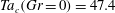 $\mathit{Ta}_{c}(\mathit{Gr}=0)=47.4$
for
$\mathit{Ta}_{c}(\mathit{Gr}=0)=47.4$
for
 ${\it\eta}=0.8$
predicted by the linear stability analysis for an infinite-length annulus. In particular, we have found the classical result that the perturbation of the azimuthal velocity component is almost 10 times larger than the radial and axial components (Drazin & Reid Reference Drazin and Reid1981). After that, we computed the velocity, vorticity and temperature fields for selected values of the Grashof number and
${\it\eta}=0.8$
predicted by the linear stability analysis for an infinite-length annulus. In particular, we have found the classical result that the perturbation of the azimuthal velocity component is almost 10 times larger than the radial and axial components (Drazin & Reid Reference Drazin and Reid1981). After that, we computed the velocity, vorticity and temperature fields for selected values of the Grashof number and
 $\mathit{Ta}<\mathit{Ta}_{c}(\mathit{Gr}=0)$
.
$\mathit{Ta}<\mathit{Ta}_{c}(\mathit{Gr}=0)$
.
We will present the data on the flow and temperature fields either in a cross-section (
 $x,z$
) or in a plane (
$x,z$
) or in a plane (
 ${\it\varphi},z$
) where
${\it\varphi},z$
) where
 $x\in [0;1]$
,
$x\in [0;1]$
,
 $z\in [0;114]$
and
$z\in [0;114]$
and
 ${\it\varphi}\in [0;2{\rm\pi}]$
.
${\it\varphi}\in [0;2{\rm\pi}]$
.
3. Results
3.1. Base flow characterization
When
 $\mathit{Ta}$
is less than the critical value
$\mathit{Ta}$
is less than the critical value
 $(\mathit{Ta}_{c})$
, a CCF is established. However, if a radial temperature gradient is additionally imposed, an axial flow develops on top of the CCF due to buoyancy. Away from the endplates, the base flow is characterized by two velocity components, which depend only on the radial coordinate
$(\mathit{Ta}_{c})$
, a CCF is established. However, if a radial temperature gradient is additionally imposed, an axial flow develops on top of the CCF due to buoyancy. Away from the endplates, the base flow is characterized by two velocity components, which depend only on the radial coordinate
 $r$
or
$r$
or
 $x$
: the azimuthal velocity component due to the rotation of the inner cylinder, and the axial velocity component induced by the radial temperature gradient. The profiles of the azimuthal and axial velocity components and the temperature of this base flow in the radial direction can be analytically obtained (Ali & Weidman Reference Ali and Weidman1990; Lepiller et al.
Reference Lepiller, Goharzadeh, Prigent and Mutabazi2008; Lopez et al.
Reference Lopez, Marques and Avila2013) as follows:
$x$
: the azimuthal velocity component due to the rotation of the inner cylinder, and the axial velocity component induced by the radial temperature gradient. The profiles of the azimuthal and axial velocity components and the temperature of this base flow in the radial direction can be analytically obtained (Ali & Weidman Reference Ali and Weidman1990; Lepiller et al.
Reference Lepiller, Goharzadeh, Prigent and Mutabazi2008; Lopez et al.
Reference Lopez, Marques and Avila2013) as follows:
 $$\begin{eqnarray}\displaystyle & \displaystyle u_{{\it\varphi}}=\frac{{\it\eta}\,\mathit{Re}}{1+{\it\eta}}\left[-r+\frac{1}{(1-{\it\eta})^{2}r}\right],\quad r=x+\frac{{\it\eta}}{1-{\it\eta}}, & \displaystyle\end{eqnarray}$$
 $$\begin{eqnarray}\displaystyle & \displaystyle u_{z}=\frac{\mathit{Gr}}{\mathit{Re}}F({\it\eta},r),\quad F({\it\eta},r)=\mathit{A}[\mathit{B}\{(1-{\it\eta})^{2}(r^{2}+T(r))-1\}-4\{(1-{\it\eta})^{2}r^{2}-{\it\eta}^{2}\}T(r)], & \displaystyle \nonumber\\ \displaystyle & & \displaystyle\end{eqnarray}$$
 $$\begin{eqnarray}\displaystyle & \displaystyle T(r)=\frac{\ln [(1-{\it\eta})r]}{\ln {\it\eta}}, & \displaystyle\end{eqnarray}$$
with the coefficients
 $A$
and
$A$
and
 $B$
given by
$B$
given by
 $$\begin{eqnarray}\displaystyle A=\frac{1}{16(1-{\it\eta})^{2}},\quad B=\frac{(1-{\it\eta}^{2})(1-3{\it\eta}^{2})-4{\it\eta}^{4}\ln {\it\eta}}{(1-{\it\eta}^{2})^{2}+(1-{\it\eta}^{4})\ln {\it\eta}}. & & \displaystyle\end{eqnarray}$$
Figure 2 shows the profiles of the velocity components and temperature computed at the mid-height (
 $z={\it\Gamma}/2$
) for
$z={\it\Gamma}/2$
) for
 $\mathit{Ta}=20$
and
$\mathit{Ta}=20$
and
 $\mathit{Gr}=250$
. They fit the profiles computed analytically assuming that the system has an infinite axial extension (Lepiller et al.
Reference Lepiller, Goharzadeh, Prigent and Mutabazi2008). From (2.2) and (2.3), one verifies that the radial temperature gradient both generates the baroclinic component of the vorticity and modifies the pressure distribution in the base flow (Lopez et al.
Reference Lopez, Marques and Avila2013).
$\mathit{Gr}=250$
. They fit the profiles computed analytically assuming that the system has an infinite axial extension (Lepiller et al.
Reference Lepiller, Goharzadeh, Prigent and Mutabazi2008). From (2.2) and (2.3), one verifies that the radial temperature gradient both generates the baroclinic component of the vorticity and modifies the pressure distribution in the base flow (Lopez et al.
Reference Lopez, Marques and Avila2013).

Figure 2. Base flow profiles at the mid-height of the flow system (
 $\mathit{Ta}=20$
,
$\mathit{Ta}=20$
,
 $\mathit{Gr}=250$
): (a) azimuthal velocity; (b) axial velocity; and (c) temperature.
$\mathit{Gr}=250$
): (a) azimuthal velocity; (b) axial velocity; and (c) temperature.
In the base flow, the friction coefficients on the inner cylinder surface are given by
 $$\begin{eqnarray}C_{M_{z}}=\frac{1}{{\it\eta}(1+{\it\eta})}\left(\frac{1-{\it\eta}}{{\it\eta}}\right)^{1/2}\frac{8}{\mathit{Ta}},\quad C_{M_{{\it\varphi}}}=\left.\frac{4\mathit{Gr}}{\mathit{Re}^{2}}\frac{\text{d}F}{\text{d}r}\right|_{r={\it\eta}/(1-{\it\eta})}.\end{eqnarray}$$
The radial and the vertical heat current densities are
 $$\begin{eqnarray}J_{r}^{cond}=-\frac{1}{r\ln {\it\eta}},\quad J_{z}^{cond}=\frac{\mathit{Gr}}{\mathit{Re}}\int _{\bar{a}}^{\bar{b}}rF({\it\eta},r)T(r)\text{d}r=\text{const}.\end{eqnarray}$$

Figure 3. Magnified view of streamlines near the top and bottom endplates: (a)
 $\mathit{Ta}=20$
,
$\mathit{Ta}=20$
,
 $\mathit{Gr}=0$
; (b)
$\mathit{Gr}=0$
; (b)
 $\mathit{Ta}=40$
,
$\mathit{Ta}=40$
,
 $\mathit{Gr}=0$
; (c)
$\mathit{Gr}=0$
; (c)
 $\mathit{Ta}=0$
,
$\mathit{Ta}=0$
,
 $\mathit{Gr}=250$
; (d)
$\mathit{Gr}=250$
; (d)
 $\mathit{Ta}=20$
,
$\mathit{Ta}=20$
,
 $\mathit{Gr}=250$
; (e)
$\mathit{Gr}=250$
; (e)
 $\mathit{Ta}=40$
,
$\mathit{Ta}=40$
,
 $\mathit{Gr}=250$
.
$\mathit{Gr}=250$
.
Near the endplates, the temperature and velocity fields depend on both the radial and the axial coordinates. For isothermal flow, the Ekman pumping (Czarny et al.
Reference Czarny, Serre, Bontoux and Lueptow2003) results in two counter-rotating vortices near the top and bottom endplates (figure 3
a,b). The flow is symmetric with respect to the plane
 $z={\it\Gamma}/2$
. The temperature gradient has a drastic effect on the Ekman pumping. For weak values of
$z={\it\Gamma}/2$
. The temperature gradient has a drastic effect on the Ekman pumping. For weak values of
 $\mathit{Ta}$
, the Ekman pumping is damped by the temperature gradient because of the formation of the convective cell (figure 3
c). The increase of
$\mathit{Ta}$
, the Ekman pumping is damped by the temperature gradient because of the formation of the convective cell (figure 3
c). The increase of
 $\mathit{Ta}$
leads to the formation of a corner vortex, which is superimposed on the convective cell (figure 3
d). This corner cell has a circulation that is opposite to that of the large convection cell; it forms in the top corner of the hot surface for
$\mathit{Ta}$
leads to the formation of a corner vortex, which is superimposed on the convective cell (figure 3
d). This corner cell has a circulation that is opposite to that of the large convection cell; it forms in the top corner of the hot surface for
 $\mathit{Gr }>0$
and in the bottom of the cold surface when
$\mathit{Gr }>0$
and in the bottom of the cold surface when
 $\mathit{Gr}<0$
. The Ekman pumping then becomes significant. The coupling of radial temperature gradient and rotation induces an asymmetry of the base flow state, which is responsible for the initiation of vortex generation near the bottom observed in experiments (Lepiller et al.
Reference Lepiller, Yoon, Prigent, Yang and Mutabazi2006, Reference Lepiller, Goharzadeh, Prigent and Mutabazi2008). At the bottom, the Ekman pumping is weakened by the thermal gradient, so that the instability develops there first, while it is very active near the top endplate when
$\mathit{Gr}<0$
. The Ekman pumping then becomes significant. The coupling of radial temperature gradient and rotation induces an asymmetry of the base flow state, which is responsible for the initiation of vortex generation near the bottom observed in experiments (Lepiller et al.
Reference Lepiller, Yoon, Prigent, Yang and Mutabazi2006, Reference Lepiller, Goharzadeh, Prigent and Mutabazi2008). At the bottom, the Ekman pumping is weakened by the thermal gradient, so that the instability develops there first, while it is very active near the top endplate when
 $\mathit{Gr}$
increases, and therefore retards the development of instability in that zone. In the case of natural convection (i.e. when
$\mathit{Gr}$
increases, and therefore retards the development of instability in that zone. In the case of natural convection (i.e. when
 $\mathit{Ta}=0$
), the base flow is symmetric and the pattern is formed in the central region of the flow (Lepiller et al.
Reference Lepiller, Prigent, Dumouchel and Mutabazi2007).
$\mathit{Ta}=0$
), the base flow is symmetric and the pattern is formed in the central region of the flow (Lepiller et al.
Reference Lepiller, Prigent, Dumouchel and Mutabazi2007).
The secondary vortex, generated by centrifugal potential, grows in size and intensity as
 $\mathit{Ta}$
increases (figure 3
e). The vortex is formed as a result of the axial variation of the radial velocity component and of the temperature near the endplate (figure 4) and their interaction with the axial vorticity component from the CCF. The top–bottom asymmetry comes from the invariance of the axial Couette flow and of the axial temperature gradient with the sign of
$\mathit{Ta}$
increases (figure 3
e). The vortex is formed as a result of the axial variation of the radial velocity component and of the temperature near the endplate (figure 4) and their interaction with the axial vorticity component from the CCF. The top–bottom asymmetry comes from the invariance of the axial Couette flow and of the axial temperature gradient with the sign of
 $\mathit{Gr}$
while the radial component changes its sign. In the case of natural convection (
$\mathit{Gr}$
while the radial component changes its sign. In the case of natural convection (
 $\mathit{Ta}=0$
), the velocity profile possesses a reflection symmetry with respect of the planes
$\mathit{Ta}=0$
), the velocity profile possesses a reflection symmetry with respect of the planes
 $x=1/2$
and
$x=1/2$
and
 $z={\it\Gamma}/2$
. The isotherms are straight vertical lines in the central part. We computed the vertical temperature gradient in the subcritical flow regime (
$z={\it\Gamma}/2$
. The isotherms are straight vertical lines in the central part. We computed the vertical temperature gradient in the subcritical flow regime (
 $\mathit{Gr}=750$
,
$\mathit{Gr}=750$
,
 $\mathit{Ta}=20$
) on the central surface
$\mathit{Ta}=20$
) on the central surface
 $x=1/2$
(figure 4): it is zero everywhere except near the endplates, where a thermal boundary layer must exist to match the adiabatic conditions. The thickness of the thermal boundary layer (the zone where
$x=1/2$
(figure 4): it is zero everywhere except near the endplates, where a thermal boundary layer must exist to match the adiabatic conditions. The thickness of the thermal boundary layer (the zone where
 $\text{d}T/\text{d}z\neq 0$
) is
$\text{d}T/\text{d}z\neq 0$
) is
 ${\it\delta}_{th}\approx 0.10{\it\Gamma}$
, while that of the hydrodynamic boundary layer (the zone where
${\it\delta}_{th}\approx 0.10{\it\Gamma}$
, while that of the hydrodynamic boundary layer (the zone where
 $u_{r}\neq 0$
) is
$u_{r}\neq 0$
) is
 ${\it\delta}_{h}\approx 0.07{\it\Gamma}$
. So the flow has sufficient length (
${\it\delta}_{h}\approx 0.07{\it\Gamma}$
. So the flow has sufficient length (
 ${\approx}0.8{\it\Gamma}$
) to develop instabilities without being influenced by end effects.
${\approx}0.8{\it\Gamma}$
) to develop instabilities without being influenced by end effects.

Figure 4. (a) Temperature gradient and (b) radial velocity component in the base flow state for
 $\mathit{Ta}=20$
,
$\mathit{Ta}=20$
,
 $\mathit{Gr}=750$
at
$\mathit{Gr}=750$
at
 $x=1/2$
. Insets are the magnified zone near the bottom endplate. The symbols represent grid points.
$x=1/2$
. Insets are the magnified zone near the bottom endplate. The symbols represent grid points.
3.2. Vortex formation and temperature field
The transition scenario from the base flow to the state with vortices depends on the values of the control parameters
 $\mathit{Ta}$
and
$\mathit{Ta}$
and
 $\mathit{Gr}$
. The numerical protocol in this study was to choose a value of
$\mathit{Gr}$
. The numerical protocol in this study was to choose a value of
 $\mathit{Ta}$
in the base state (i.e. without vortex structure) and then fix the suitable value of
$\mathit{Ta}$
in the base state (i.e. without vortex structure) and then fix the suitable value of
 $\mathit{Gr}$
and wait for the occurrence of the pattern. The established flow state is reached when the torque and heat transfer coefficient do not vary any more in time. The same protocol was used by Kedia et al. (Reference Kedia, Hunt and Colonius1998), while Kuo & Ball (Reference Kuo and Ball1997) fixed
$\mathit{Gr}$
and wait for the occurrence of the pattern. The established flow state is reached when the torque and heat transfer coefficient do not vary any more in time. The same protocol was used by Kedia et al. (Reference Kedia, Hunt and Colonius1998), while Kuo & Ball (Reference Kuo and Ball1997) fixed
 $\mathit{Gr}$
and varied
$\mathit{Gr}$
and varied
 $\mathit{Ta}$
. For the isothermal flow, i.e.
$\mathit{Ta}$
. For the isothermal flow, i.e.
 $\mathit{Gr}=0$
, stationary axisymmetric vortices appear at
$\mathit{Gr}=0$
, stationary axisymmetric vortices appear at
 $\mathit{Ta}_{c}=48$
, which is almost the value predicted by linear stability theory for an infinite-length annulus (
$\mathit{Ta}_{c}=48$
, which is almost the value predicted by linear stability theory for an infinite-length annulus (
 $\mathit{Ta}_{c}=47.4$
). Compared to the simulations of Kuo & Ball (Reference Kuo and Ball1997) performed in a small-aspect-ratio system (
$\mathit{Ta}_{c}=47.4$
). Compared to the simulations of Kuo & Ball (Reference Kuo and Ball1997) performed in a small-aspect-ratio system (
 ${\it\Gamma}=31.5$
), in which the bifurcation was imperfect for
${\it\Gamma}=31.5$
), in which the bifurcation was imperfect for
 $65<\mathit{Ta}<70$
, in our flow system, the imperfections induced by the Ekman cells into the bifurcation are negligible because of the large aspect ratio. The influence of the aspect ratio on the threshold in the isothermal Taylor–Couette flow has recently been revisited by different authors, and it was shown that the characteristic time of the critical mode varies with the aspect ratio as
$65<\mathit{Ta}<70$
, in our flow system, the imperfections induced by the Ekman cells into the bifurcation are negligible because of the large aspect ratio. The influence of the aspect ratio on the threshold in the isothermal Taylor–Couette flow has recently been revisited by different authors, and it was shown that the characteristic time of the critical mode varies with the aspect ratio as
 ${\it\Gamma}^{-2}$
(Manneville & Czarny Reference Manneville and Czarny2009). The stability of the non-rotating annulus (
${\it\Gamma}^{-2}$
(Manneville & Czarny Reference Manneville and Czarny2009). The stability of the non-rotating annulus (
 $\mathit{Ta}=0$
) has been widely investigated by many authors (Choi & Korpela Reference Choi and Korpela1980; Le Quéré & Pécheux Reference Le Quéré and Pécheux1989; Bahloul, Mutabazi & Ambari Reference Bahloul, Mutabazi and Ambari2000; Lepiller et al.
Reference Lepiller, Prigent, Dumouchel and Mutabazi2007) and is not reproduced in the present study.
$\mathit{Ta}=0$
) has been widely investigated by many authors (Choi & Korpela Reference Choi and Korpela1980; Le Quéré & Pécheux Reference Le Quéré and Pécheux1989; Bahloul, Mutabazi & Ambari Reference Bahloul, Mutabazi and Ambari2000; Lepiller et al.
Reference Lepiller, Prigent, Dumouchel and Mutabazi2007) and is not reproduced in the present study.
We performed computations for
 $\mathit{Ta}<\mathit{Ta}_{c}$
and
$\mathit{Ta}<\mathit{Ta}_{c}$
and
 $|\mathit{Gr}|\in [0,2500]$
; but, for conciseness, we will focus on the results obtained for
$|\mathit{Gr}|\in [0,2500]$
; but, for conciseness, we will focus on the results obtained for
 $\mathit{Ta}=40$
. The patterns obtained for any pair (
$\mathit{Ta}=40$
. The patterns obtained for any pair (
 $\mathit{Gr},-\mathit{Gr}$
) have opposite helicity, in accordance with the symmetry arguments developed by Ali & Weidman (Reference Ali and Weidman1990). We verified that the pattern orientation depends on the sign of the product
$\mathit{Gr},-\mathit{Gr}$
) have opposite helicity, in accordance with the symmetry arguments developed by Ali & Weidman (Reference Ali and Weidman1990). We verified that the pattern orientation depends on the sign of the product
 $\mathit{Gr}\,\mathit{Ta}$
. As
$\mathit{Gr}\,\mathit{Ta}$
. As
 $|\mathit{Gr}|$
increases from the base flow state, the large convective cell becomes unstable and gives rise to the formation of co-rotating vortices (figure 5
b). For
$|\mathit{Gr}|$
increases from the base flow state, the large convective cell becomes unstable and gives rise to the formation of co-rotating vortices (figure 5
b). For
 $\mathit{Ta}=40$
, they were obtained around
$\mathit{Ta}=40$
, they were obtained around
 $\mathit{Gr}=290$
. These vortices travel along and around the inner cylinder with a velocity that depends on the values of
$\mathit{Gr}=290$
. These vortices travel along and around the inner cylinder with a velocity that depends on the values of
 $\mathit{Gr}$
and
$\mathit{Gr}$
and
 $\mathit{Ta}$
. The circulation of the vortices is determined by the large convective cell: it is positive when the inner cylinder is heated and negative when the outer is heated. Co-rotating vortices have been reported in previous numerical studies (Kuo & Ball Reference Kuo and Ball1997; Kedia et al.
Reference Kedia, Hunt and Colonius1998). A further increase of
$\mathit{Ta}$
. The circulation of the vortices is determined by the large convective cell: it is positive when the inner cylinder is heated and negative when the outer is heated. Co-rotating vortices have been reported in previous numerical studies (Kuo & Ball Reference Kuo and Ball1997; Kedia et al.
Reference Kedia, Hunt and Colonius1998). A further increase of
 $\mathit{Gr}$
leads to the appearance of small counter-rotating vortices (figure 5
c) of uneven size (the new vortices have a smaller size and a negative vorticity). The precise value of
$\mathit{Gr}$
leads to the appearance of small counter-rotating vortices (figure 5
c) of uneven size (the new vortices have a smaller size and a negative vorticity). The precise value of
 $\mathit{Gr}$
for which the transition between co-rotating and counter-rotating vortices occurs has not been determined accurately because of the large CPU time needed for such a task. For
$\mathit{Gr}$
for which the transition between co-rotating and counter-rotating vortices occurs has not been determined accurately because of the large CPU time needed for such a task. For
 $\mathit{Ta}=40$
, they appear around
$\mathit{Ta}=40$
, they appear around
 $\mathit{Gr}=690$
.
$\mathit{Gr}=690$
.

Figure 5. Contours of azimuthal vorticity to show flow structures in the central part of the annulus for
 $\mathit{Ta }=40$
with different values of
$\mathit{Ta }=40$
with different values of
 $\mathit{Gr}$
: (a)
$\mathit{Gr}$
: (a)
 $\mathit{Gr}=250$
; (b)
$\mathit{Gr}=250$
; (b)
 $\mathit{Gr}=290$
; (c)
$\mathit{Gr}=290$
; (c)
 $\mathit{Gr}=750$
; (d)
$\mathit{Gr}=750$
; (d)
 $\mathit{Gr}=1000$
; (e)
$\mathit{Gr}=1000$
; (e)
 $\mathit{Gr}=1500$
.
$\mathit{Gr}=1500$
.
The alternation of positive and negative vortices of uneven size leads to modulation in patterns for larger values of
 $\mathit{Gr}$
. Their propagation also induces collisions that accelerate the occurrence of the chaotic pattern (figure 5
d,e). The strength of the vortices increases with the increase of
$\mathit{Gr}$
. Their propagation also induces collisions that accelerate the occurrence of the chaotic pattern (figure 5
d,e). The strength of the vortices increases with the increase of
 $\mathit{Gr}$
.
$\mathit{Gr}$
.
The isotherms in the central part of the system are represented in figure 6. They are straight lines in the base flow and are undulating lines for co-rotating vortices. When counter-rotating vortices are formed (for
 $\mathit{Gr }>690$
), thermal plumes appear near the hot cylindrical surface and penetrate into the cold zones. They are accompanied by strong horizontal and vertical temperature gradients that enhance the vorticity and the pressure, respectively.
$\mathit{Gr }>690$
), thermal plumes appear near the hot cylindrical surface and penetrate into the cold zones. They are accompanied by strong horizontal and vertical temperature gradients that enhance the vorticity and the pressure, respectively.

Figure 6. Instantaneous temperature contours on
 $r{-}z$
plane for
$r{-}z$
plane for
 $\mathit{Ta}=40$
: (a)
$\mathit{Ta}=40$
: (a)
 $\mathit{Gr}=250$
; (b)
$\mathit{Gr}=250$
; (b)
 $\mathit{Gr}=290$
; (c)
$\mathit{Gr}=290$
; (c)
 $\mathit{Gr}=750$
; (d)
$\mathit{Gr}=750$
; (d)
 $\mathit{Gr}=1000$
; (e)
$\mathit{Gr}=1000$
; (e)
 $\mathit{Gr}=1500$
.
$\mathit{Gr}=1500$
.
Representation of pattern structure can be made by using either streamlines or isovalues of any component of velocity or vorticity or the isotherms. Using the isovalues of azimuthal vorticity, we represented the three-dimensional cores of vortical structures (figure 7) and they compare well with the isovalues of the vorticity (figure 5). Figure 7(a) illustrates the co-rotating vortices while figure 7(b) shows the counter-rotating spirals. In figure 7(c,d), one observes the destruction or creation of a vortex in the flow.

Figure 7. Cores of the azimuthal vorticity in the central part of the flow system for
 $\mathit{Ta}=40$
: (a)
$\mathit{Ta}=40$
: (a)
 $\mathit{Gr}=290$
(
$\mathit{Gr}=290$
(
 ${\it\omega}_{{\it\varphi}}=0.13$
); (b)
${\it\omega}_{{\it\varphi}}=0.13$
); (b)
 $\mathit{Gr}=750$
(
$\mathit{Gr}=750$
(
 ${\it\omega}_{{\it\varphi}}=0.3,-0.1$
); (c)
${\it\omega}_{{\it\varphi}}=0.3,-0.1$
); (c)
 $\mathit{Gr}=1000$
(
$\mathit{Gr}=1000$
(
 ${\it\omega}_{{\it\varphi}}=0.35,-0.15$
); (d)
${\it\omega}_{{\it\varphi}}=0.35,-0.15$
); (d)
 $\mathit{Gr}=1500$
(
$\mathit{Gr}=1500$
(
 ${\it\omega}_{{\it\varphi}}=0.4,-0.25$
) (red, positive; blue, negative).
${\it\omega}_{{\it\varphi}}=0.4,-0.25$
) (red, positive; blue, negative).

Figure 8. Instantaneous contours of axial velocity component on the centre surface of the annulus (
 $x=1/2,{\it\varphi},z$
) for
$x=1/2,{\it\varphi},z$
) for
 $\mathit{Ta}=40$
: (a)
$\mathit{Ta}=40$
: (a)
 $\mathit{Gr}=290$
; (b)
$\mathit{Gr}=290$
; (b)
 $\mathit{Gr}=750$
; (c)
$\mathit{Gr}=750$
; (c)
 $\mathit{Gr}=1000$
; (d)
$\mathit{Gr}=1000$
; (d)
 $\mathit{Gr}=1500$
.
$\mathit{Gr}=1500$
.

Figure 9. (a–c) Space–time diagrams of the temperature and (d–f) the corresponding frequency spectra averaged over the spatial coordinate
 $z$
for
$z$
for
 $\mathit{Ta}=40$
: (a,d)
$\mathit{Ta}=40$
: (a,d)
 $\mathit{Gr}=500$
; (b,e)
$\mathit{Gr}=500$
; (b,e)
 $\mathit{Gr}=1000$
; (c, f)
$\mathit{Gr}=1000$
; (c, f)
 $\mathit{Gr}=2000$
. (g–i) The phase portraits (
$\mathit{Gr}=2000$
. (g–i) The phase portraits (
 $u_{r},\text{d}u_{r}/\text{d}r$
) during the time span of
$u_{r},\text{d}u_{r}/\text{d}r$
) during the time span of
 ${\rm\Delta}t=6.0$
at
${\rm\Delta}t=6.0$
at
 $x=1/2$
,
$x=1/2$
,
 ${\it\varphi}={\rm\pi}$
and
${\it\varphi}={\rm\pi}$
and
 $z={\it\Gamma}/2$
for the same values of
$z={\it\Gamma}/2$
for the same values of
 $\mathit{Gr}$
.
$\mathit{Gr}$
.
3.3. Spatio-temporal properties of convective flows
In order to determine the axial and azimuthal wavenumbers, we have plotted the isovalues of the axial velocity computed at the central lateral surface
 $x=1/2$
(figure 8). We found that the azimuthal wavenumber
$x=1/2$
(figure 8). We found that the azimuthal wavenumber
 $m$
takes values from 2 to 5, while the axial wavenumber varies between 1.652 and 2.701 depending on the values of
$m$
takes values from 2 to 5, while the axial wavenumber varies between 1.652 and 2.701 depending on the values of
 $\mathit{Ta}$
and
$\mathit{Ta}$
and
 $\mathit{Gr}$
(table 1). The sign change of
$\mathit{Gr}$
(table 1). The sign change of
 $\mathit{Gr}$
induces the inversion of the spiral helicity. Figure 8(b–d) illustrates the splitting of one vortex into two vortices and merging of two vortices into one vortex in the central part of the flow system. These events lead to the low frequency in the power spectra (figure 9
e, f), which are not observed for a pure periodic pattern for small values of
$\mathit{Gr}$
induces the inversion of the spiral helicity. Figure 8(b–d) illustrates the splitting of one vortex into two vortices and merging of two vortices into one vortex in the central part of the flow system. These events lead to the low frequency in the power spectra (figure 9
e, f), which are not observed for a pure periodic pattern for small values of
 $\mathit{Gr}$
(figure 9
d).
$\mathit{Gr}$
(figure 9
d).
Table 1. Values of frequency and wavenumber for
 $\mathit{Ta}=40$
.
$\mathit{Ta}=40$
.

The variation in time and axial direction of the flow pattern is exhibited in the form of a space–time diagram (figure 9
a–c), from which we have extracted the frequency and axial wavenumber by a fast Fourier transform. For small values of
 $\mathit{Gr}$
, the pattern spectra exhibit only one peak corresponding to the oscillation frequency or to the wavenumber of vortices (figure 9
d). The corresponding phase portrait is a closed loop (figure 9
g) illustrating the mono-periodicity of the flow. For large values of
$\mathit{Gr}$
, the pattern spectra exhibit only one peak corresponding to the oscillation frequency or to the wavenumber of vortices (figure 9
d). The corresponding phase portrait is a closed loop (figure 9
g) illustrating the mono-periodicity of the flow. For large values of
 $\mathit{Gr}$
, the spectra exhibit either bi-periodic character or chaotic behaviour (figure 9
e, f) coming from the propagation of vortices of uneven size and the presence of defects (figure 9
h). We identified in the spectra the peak of the fundamental frequency
$\mathit{Gr}$
, the spectra exhibit either bi-periodic character or chaotic behaviour (figure 9
e, f) coming from the propagation of vortices of uneven size and the presence of defects (figure 9
h). We identified in the spectra the peak of the fundamental frequency
 $f_{0}$
and two side peaks away from the fundamental one by
$f_{0}$
and two side peaks away from the fundamental one by
 ${\rm\Delta}f_{0}$
. The main peak corresponds to the co-rotating vortices while the side peaks correspond to the counter-rotating vortices of uneven size. For
${\rm\Delta}f_{0}$
. The main peak corresponds to the co-rotating vortices while the side peaks correspond to the counter-rotating vortices of uneven size. For
 $\mathit{Gr}=2000$
, the spectrum (figure 9
f) exhibits a large background noise due to the splitting and merging of vortices. The appearance of chaotic behaviour is clearly identified by the dense phase portrait in figure 9(i). The frequencies (
$\mathit{Gr}=2000$
, the spectrum (figure 9
f) exhibits a large background noise due to the splitting and merging of vortices. The appearance of chaotic behaviour is clearly identified by the dense phase portrait in figure 9(i). The frequencies (
 $f_{0}$
and
$f_{0}$
and
 ${\rm\Delta}f_{0}$
) and the axial wavenumber do not vary significantly with the rotation rate (
${\rm\Delta}f_{0}$
) and the axial wavenumber do not vary significantly with the rotation rate (
 $\mathit{Ta}$
), while they do vary with
$\mathit{Ta}$
), while they do vary with
 $\mathit{Gr}$
; this is a signature that they are induced by a buoyancy effect (figure 10).
$\mathit{Gr}$
; this is a signature that they are induced by a buoyancy effect (figure 10).

Figure 10. Variation with
 $\mathit{Ta}$
of (a) the pattern dimensionless frequency for
$\mathit{Ta}$
of (a) the pattern dimensionless frequency for
 $\mathit{Gr}=1000$
, and (b) the wavenumber for
$\mathit{Gr}=1000$
, and (b) the wavenumber for
 $\mathit{Gr}=1000$
and
$\mathit{Gr}=1000$
and
 $\mathit{Gr}=2000$
.
$\mathit{Gr}=2000$
.
Table 2. Averaged values of the friction coefficients and Nusselt number at the inner cylinder for
 $\mathit{Ta}=40$
.
$\mathit{Ta}=40$
.

3.4. Torque and heat transfer
We computed the coefficient of the momentum transfer on the inner cylinder surface for different values of
 $\mathit{Gr}$
and
$\mathit{Gr}$
and
 $\mathit{Ta}=40$
; the data are plotted in figure 11(a) and given in table 2. Here the overbar means averaging in time. For isothermal flow (
$\mathit{Ta}=40$
; the data are plotted in figure 11(a) and given in table 2. Here the overbar means averaging in time. For isothermal flow (
 $\mathit{Gr}=0$
), the value of the momentum coefficient computed by direct numerical simulations (DNS),
$\mathit{Gr}=0$
), the value of the momentum coefficient computed by direct numerical simulations (DNS),
 $C_{M_{z}}^{DNS}=0.07137$
, compares well with the theoretical value obtained for CCF (3.2a,b
) with infinite-length cylinders (Dubrulle & Hersant Reference Dubrulle and Hersant2002; Childs Reference Childs2010),
$C_{M_{z}}^{DNS}=0.07137$
, compares well with the theoretical value obtained for CCF (3.2a,b
) with infinite-length cylinders (Dubrulle & Hersant Reference Dubrulle and Hersant2002; Childs Reference Childs2010),
 $C_{M_{z}}^{\infty }=0.06944$
. The discrepancy of 2.8 % between these values may arise from endplate effects. The azimuthal torque for
$C_{M_{z}}^{\infty }=0.06944$
. The discrepancy of 2.8 % between these values may arise from endplate effects. The azimuthal torque for
 $|\mathit{Gr}|=250$
is the same as the isothermal value because the corresponding flow has no vortices except the large convective cell. But as soon as the large convective cell becomes unstable for
$|\mathit{Gr}|=250$
is the same as the isothermal value because the corresponding flow has no vortices except the large convective cell. But as soon as the large convective cell becomes unstable for
 $|\mathit{Gr}|\approx 290$
and gives rise to secondary convective vortices, then the values of
$|\mathit{Gr}|\approx 290$
and gives rise to secondary convective vortices, then the values of
 $\bar{C}_{M_{z}}$
grow to approximately 17 % for
$\bar{C}_{M_{z}}$
grow to approximately 17 % for
 $|\mathit{Gr}|=2500$
compared to the isothermal torque in the base flow state. This increase is associated with the appearance of secondary vortices in the convective flow patterns.
$|\mathit{Gr}|=2500$
compared to the isothermal torque in the base flow state. This increase is associated with the appearance of secondary vortices in the convective flow patterns.

Figure 11. Variation of time-averaged transfer coefficients at the inner cylinder with
 $\mathit{Gr}$
for
$\mathit{Gr}$
for
 $\mathit{Ta}=40$
: (a) friction coefficients; and (b) mean Nusselt number
$\mathit{Ta}=40$
: (a) friction coefficients; and (b) mean Nusselt number
 $\overline{\mathit{Nu}}_{i}$
.
$\overline{\mathit{Nu}}_{i}$
.
The temperature difference creates a new component of the torque with a corresponding friction coefficient
 $\bar{C}_{M_{{\it\varphi}}}$
given by the formula (2.10) and plotted in figure 11(a). This coefficient increases with
$\bar{C}_{M_{{\it\varphi}}}$
given by the formula (2.10) and plotted in figure 11(a). This coefficient increases with
 $\mathit{Gr}$
and becomes comparable with the rotation torque for
$\mathit{Gr}$
and becomes comparable with the rotation torque for
 $\mathit{Gr}>1500$
.
$\mathit{Gr}>1500$
.
The heat transfer at the inner cylinder surface was computed through the Nusselt number defined by the relations (2.15a,b
), and the transfer at the outer cylinder is
 $\mathit{Nu}_{o}={\it\eta}\mathit{Nu}_{i}$
because the slope of the temperature near the cylindrical surfaces is almost the same. The mean Nusselt number increases as the Grashof number increases up to
$\mathit{Nu}_{o}={\it\eta}\mathit{Nu}_{i}$
because the slope of the temperature near the cylindrical surfaces is almost the same. The mean Nusselt number increases as the Grashof number increases up to
 $|\mathit{Gr}|\approx 1000$
and then saturates (figure 11
b). Some authors use the equivalent conductivity (Kedia et al.
Reference Kedia, Hunt and Colonius1998), which is related to the Nusselt number by
$|\mathit{Gr}|\approx 1000$
and then saturates (figure 11
b). Some authors use the equivalent conductivity (Kedia et al.
Reference Kedia, Hunt and Colonius1998), which is related to the Nusselt number by
 $K_{eq}=2\mathit{Nu}_{i}$
. The mean values of momentum transport and heat transfer are almost symmetric with respect to
$K_{eq}=2\mathit{Nu}_{i}$
. The mean values of momentum transport and heat transfer are almost symmetric with respect to
 $\mathit{Gr}=0$
(table 2), i.e. heating the inner or the outer cylinder does not modify the value of the torque and the heat transfer on the inner cylinder. This quasi-symmetric behaviour of the friction coefficients and of the heat transfer coefficient is due to the weak value of the centrifugal buoyancy parameter (
$\mathit{Gr}=0$
(table 2), i.e. heating the inner or the outer cylinder does not modify the value of the torque and the heat transfer on the inner cylinder. This quasi-symmetric behaviour of the friction coefficients and of the heat transfer coefficient is due to the weak value of the centrifugal buoyancy parameter (
 $\mathit{Ga}^{-1}\sim 10^{-7}$
) for the flow investigated in this system (Yoshikawa et al.
Reference Yoshikawa, Nagata and Mutabazi2013).
$\mathit{Ga}^{-1}\sim 10^{-7}$
) for the flow investigated in this system (Yoshikawa et al.
Reference Yoshikawa, Nagata and Mutabazi2013).
The axial flow is accompanied by a vertical heat flux that was computed using the relation (2.16). The results are plotted in figure 12 for
 $\mathit{Ta}=40$
and three values of
$\mathit{Ta}=40$
and three values of
 $\mathit{Gr}$
corresponding to the laminar state
$\mathit{Gr}$
corresponding to the laminar state
 $(\mathit{Gr}=250)$
, the regime of co-rotating vortices
$(\mathit{Gr}=250)$
, the regime of co-rotating vortices
 $(\mathit{Gr}=290)$
and the regime of counter-rotating vortices
$(\mathit{Gr}=290)$
and the regime of counter-rotating vortices
 $(\mathit{Gr}=1000)$
. In the cases of
$(\mathit{Gr}=1000)$
. In the cases of
 $\mathit{Gr}=250$
and 290, the vertical heat flux is constant in the central part of the flow as
$\mathit{Gr}=250$
and 290, the vertical heat flux is constant in the central part of the flow as
 $\bar{Q}_{z}=8.793$
and 9.837, respectively. However, for
$\bar{Q}_{z}=8.793$
and 9.837, respectively. However, for
 $\mathit{Gr}=1000$
,
$\mathit{Gr}=1000$
,
 $\bar{Q}_{z}$
varies in the central part around a value much less than
$\bar{Q}_{z}$
varies in the central part around a value much less than
 $Q_{z}^{lam}=34.077$
for an infinite-length annulus owing to the counter-rotating vortices formed in the annulus. For each value of
$Q_{z}^{lam}=34.077$
for an infinite-length annulus owing to the counter-rotating vortices formed in the annulus. For each value of
 $\mathit{Gr}$
, it drops rapidly in the boundary layers and vanishes at the endplates because of the boundary conditions (2.17). Near the top endplate for
$\mathit{Gr}$
, it drops rapidly in the boundary layers and vanishes at the endplates because of the boundary conditions (2.17). Near the top endplate for
 $\mathit{Gr}=250$
and 290, there is a sign reversal because of the presence of the recirculation cell with an anticlockwise circulation opposite to the large cell circulation.
$\mathit{Gr}=250$
and 290, there is a sign reversal because of the presence of the recirculation cell with an anticlockwise circulation opposite to the large cell circulation.

Figure 12. (a) Time-averaged total heat flux across the
 $r{-}{\it\varphi}$
plane for
$r{-}{\it\varphi}$
plane for
 $\mathit{Ta}=40$
for three values of
$\mathit{Ta}=40$
for three values of
 $\mathit{Gr}$
. (b,c) Enlarged views of the curve for
$\mathit{Gr}$
. (b,c) Enlarged views of the curve for
 $\mathit{Gr}=250$
near the bottom and the top, respectively.
$\mathit{Gr}=250$
near the bottom and the top, respectively.
4. Discussion
4.1. Comparison with experiment
The present numerical results are compared with the experimental results of Lepiller et al. (Reference Lepiller, Prigent, Dumouchel and Mutabazi2007, Reference Lepiller, Goharzadeh, Prigent and Mutabazi2008) keeping in mind that, in the experiment, the value of
 $\mathit{Gr}$
was fixed and the Taylor number was increased from the base state to states with vortices. For
$\mathit{Gr}$
was fixed and the Taylor number was increased from the base state to states with vortices. For
 $\mathit{Ta}=40$
, the bifurcated state occurred at
$\mathit{Ta}=40$
, the bifurcated state occurred at
 $\mathit{Gr}\in ]\!240,300\![$
with
$\mathit{Gr}\in ]\!240,300\ ${\rm\Delta}Gr\approx 60$
and was formed of spiral vortices occupying the lower part of the flow system near the bottom end. The size of the pattern increased as the value of
${\rm\Delta}Gr\approx 60$
and was formed of spiral vortices occupying the lower part of the flow system near the bottom end. The size of the pattern increased as the value of
 $\mathit{Ta}$
was increased until the spiral vortex pattern filled the whole system. Lepiller et al. (Reference Lepiller, Goharzadeh, Prigent and Mutabazi2008) reported in their figure 4(b) that the patterns of spiral vortex flow for
$\mathit{Ta}$
was increased until the spiral vortex pattern filled the whole system. Lepiller et al. (Reference Lepiller, Goharzadeh, Prigent and Mutabazi2008) reported in their figure 4(b) that the patterns of spiral vortex flow for
 $\mathit{Gr}=390$
have the threshold
$\mathit{Gr}=390$
have the threshold
 $\mathit{Ta}^{\ast }=38.5$
, which is close to
$\mathit{Ta}^{\ast }=38.5$
, which is close to
 $\mathit{Ta}=40$
. This pattern is closer to that obtained in the numerical simulations (figure 5
b here) for
$\mathit{Ta}=40$
. This pattern is closer to that obtained in the numerical simulations (figure 5
b here) for
 $\mathit{Gr}=290$
corresponding to co-rotating vortices. As seen from figure 3, increasing the value of
$\mathit{Gr}=290$
corresponding to co-rotating vortices. As seen from figure 3, increasing the value of
 $\mathit{Ta}$
for a fixed value of
$\mathit{Ta}$
for a fixed value of
 $\mathit{Gr}$
induces an asymmetry between the bottom and the top. Therefore the instability occurs first near the bottom endplate, while near the top endplate the corner vortex delays instability formation. This is the situation encountered in experiments (Lepiller et al.
Reference Lepiller, Prigent, Dumouchel and Mutabazi2007, Reference Lepiller, Goharzadeh, Prigent and Mutabazi2008; Guillerm Reference Guillerm2010). In the present numerical simulations, the protocol is different:
$\mathit{Gr}$
induces an asymmetry between the bottom and the top. Therefore the instability occurs first near the bottom endplate, while near the top endplate the corner vortex delays instability formation. This is the situation encountered in experiments (Lepiller et al.
Reference Lepiller, Prigent, Dumouchel and Mutabazi2007, Reference Lepiller, Goharzadeh, Prigent and Mutabazi2008; Guillerm Reference Guillerm2010). In the present numerical simulations, the protocol is different:
 $\mathit{Ta}$
is fixed and
$\mathit{Ta}$
is fixed and
 $\mathit{Gr}$
is increased from the base state to convective states. Figure 3(b) shows that, for
$\mathit{Gr}$
is increased from the base state to convective states. Figure 3(b) shows that, for
 $\mathit{Ta}=40$
and
$\mathit{Ta}=40$
and
 $\mathit{Gr}=0$
, the base flow contains two similar Ekman cells (with opposite circulation) near the endplates so that the flow is symmetric with respect to the mid-plane at
$\mathit{Gr}=0$
, the base flow contains two similar Ekman cells (with opposite circulation) near the endplates so that the flow is symmetric with respect to the mid-plane at
 $z={\it\Gamma}/2$
. Imposing a temperature gradient introduces an asymmetry in the flow between the bottom and the top. However, the transition line between the base state and the vortex regime is difficult to determine numerically, as this requires a large amount of computing time.
$z={\it\Gamma}/2$
. Imposing a temperature gradient introduces an asymmetry in the flow between the bottom and the top. However, the transition line between the base state and the vortex regime is difficult to determine numerically, as this requires a large amount of computing time.
As far as stationary or periodic patterns are concerned, the wavenumbers are related to the flow geometry and are less sensitive to the protocol. A comparison between experiments (Lepiller et al.
Reference Lepiller, Goharzadeh, Prigent and Mutabazi2008) and the present numerical simulations can be made for data on the wavenumber
 $q=\sqrt{q_{z}^{2}+q_{{\it\varphi}}^{2}}$
as a function of
$q=\sqrt{q_{z}^{2}+q_{{\it\varphi}}^{2}}$
as a function of
 $\mathit{Ri}=\mathit{Gr}/\mathit{Re}^{2}$
, where
$\mathit{Ri}=\mathit{Gr}/\mathit{Re}^{2}$
, where
 $q_{{\it\varphi}}=2(1-{\it\eta})m/(1+{\it\eta})$
is the non-dimensionalized azimuthal wavenumber. The agreement between the available numerical values and those obtained in the experiment is very good (figure 13). The frequencies obtained in DNS (figure 10
a) compare well with those obtained in the experiments (figure 8 of Lepiller et al.
Reference Lepiller, Goharzadeh, Prigent and Mutabazi2008) for the same values of
$q_{{\it\varphi}}=2(1-{\it\eta})m/(1+{\it\eta})$
is the non-dimensionalized azimuthal wavenumber. The agreement between the available numerical values and those obtained in the experiment is very good (figure 13). The frequencies obtained in DNS (figure 10
a) compare well with those obtained in the experiments (figure 8 of Lepiller et al.
Reference Lepiller, Goharzadeh, Prigent and Mutabazi2008) for the same values of
 $\mathit{Ta}=40$
and
$\mathit{Ta}=40$
and
 $\mathit{Gr}=1000$
within the experimental precision.
$\mathit{Gr}=1000$
within the experimental precision.

Figure 13. Variation of the wavenumber
 $q$
with
$q$
with
 $\mathit{Ri}$
from DNS and experiments.
$\mathit{Ri}$
from DNS and experiments.
Compared to the work of Kuo & Ball (Reference Kuo and Ball1997) performed in a relatively short system, the present study deals with an extended flow system in which thermal and hydrodynamic boundary layers are confined near the endplates. Its central part has a sufficient length to ensure that the base state is in the conduction regime and that observed vortices result from the instability mechanism not polluted by end effects. However, as mentioned in § 3.1, these end effects may have a great consequence on the generation of vortices if one fixes
 $\mathit{Gr}$
and varies
$\mathit{Gr}$
and varies
 $\mathit{Ta}$
as in most of the experiments (Snyder & Karlsson Reference Snyder and Karlsson1964; Sorour & Coney Reference Sorour and Coney1979; Ball & Farouk Reference Ball and Farouk1989; Lepiller et al.
Reference Lepiller, Goharzadeh, Prigent and Mutabazi2008).
$\mathit{Ta}$
as in most of the experiments (Snyder & Karlsson Reference Snyder and Karlsson1964; Sorour & Coney Reference Sorour and Coney1979; Ball & Farouk Reference Ball and Farouk1989; Lepiller et al.
Reference Lepiller, Goharzadeh, Prigent and Mutabazi2008).
The formation of the co-rotating vortices is a consequence of the destabilization of the large convective cell of the base flow by shear instability because the velocity profile exhibits an inflection point near the central cylindrical surface (
 $x=0.5$
). According to the Rayleigh–Förtoft criterion (Drazin & Reid Reference Drazin and Reid1981), the flow is unstable to transverse perturbations, leading to Kelvin–Helmholtz instability, which manifests itself in the form of travelling vortices. The phase velocity of the co-rotating vortices along the axial direction increases with
$x=0.5$
). According to the Rayleigh–Förtoft criterion (Drazin & Reid Reference Drazin and Reid1981), the flow is unstable to transverse perturbations, leading to Kelvin–Helmholtz instability, which manifests itself in the form of travelling vortices. The phase velocity of the co-rotating vortices along the axial direction increases with
 $\mathit{Gr}$
(table 1).
$\mathit{Gr}$
(table 1).
The appearance of counter-rotating vortices when
 $\mathit{Gr}$
increases is a signature of a secondary instability mode. In the experiment of Guillerm (Reference Guillerm2010), the secondary instability mode is described as a spiral vortex flow. Such an instability mode was also detected in numerical simulations of natural convection in a vertical slot and was attributed to a pressure gradient, which causes the imbalance between the buoyancy and viscous forces (Choi & Korpela Reference Choi and Korpela1980). In fact, according to (2.3), the isotherms of co-rotating vortices (figure 6) are deformed and generate a vertical temperature gradient, which is a source of pressure, and a horizontal gradient, which is a source of vorticity. These baroclinic sources of pressure and vorticity between two vortices have to overcome the viscous dissipation in order to generate vortices rotating in the opposite direction. Guillerm (Reference Guillerm2010) observed that, for fixed
$\mathit{Gr}$
increases is a signature of a secondary instability mode. In the experiment of Guillerm (Reference Guillerm2010), the secondary instability mode is described as a spiral vortex flow. Such an instability mode was also detected in numerical simulations of natural convection in a vertical slot and was attributed to a pressure gradient, which causes the imbalance between the buoyancy and viscous forces (Choi & Korpela Reference Choi and Korpela1980). In fact, according to (2.3), the isotherms of co-rotating vortices (figure 6) are deformed and generate a vertical temperature gradient, which is a source of pressure, and a horizontal gradient, which is a source of vorticity. These baroclinic sources of pressure and vorticity between two vortices have to overcome the viscous dissipation in order to generate vortices rotating in the opposite direction. Guillerm (Reference Guillerm2010) observed that, for fixed
 $\mathit{Ta}\approx 40$
and values of
$\mathit{Ta}\approx 40$
and values of
 $\mathit{Gr}>1000$
, the spiral vortex becomes unstable to wavy spiral vortex flow and then eventually bifurcates to a chaotic pattern with many defects. In our simulations, defects were detected for
$\mathit{Gr}>1000$
, the spiral vortex becomes unstable to wavy spiral vortex flow and then eventually bifurcates to a chaotic pattern with many defects. In our simulations, defects were detected for
 $\mathit{Gr}=1000$
and 2000 (figure 7).
$\mathit{Gr}=1000$
and 2000 (figure 7).
4.2. Transfer and averaged integral values
The behaviour of the friction coefficient with the radial temperature gradient can be analysed using (2.7). According to this equation, after time averaging over a period of oscillations, and neglecting the contribution of the centrifugal buoyancy, we found that the increase of the torque compared to the isothermal case is due to the Archimedean buoyancy power production
 $(\langle \mathit{Tu}_{z}\rangle _{V}<0)$
through the relation
$(\langle \mathit{Tu}_{z}\rangle _{V}<0)$
through the relation
 $$\begin{eqnarray}C_{M_{z}}=\frac{2(1+{\it\eta})}{{\it\eta}}\left[\frac{{\it\varepsilon}}{\mathit{Re}}-\frac{\mathit{Gr}}{\mathit{Re}^{2}}\langle \mathit{Tu}_{z}\rangle _{V}\right].\end{eqnarray}$$
The transport of momentum along the axial direction is related to the azimuthal vorticity; it vanishes in isothermal flow. This momentum transport is associated with the vertical heat flux (figure 12). The existence of this momentum induced by the temperature gradient was pointed out by Auer et al. (Reference Auer, Busse and Gangler1996) using a weakly nonlinear analysis.
The heat transfer across the cylinder surface increases with
 $\mathit{Gr}$
as long as the flow is formed either of the large convective cell or of co-rotating vortices. In this case, the heat transfer is ensured by the large convective cell. For
$\mathit{Gr}$
as long as the flow is formed either of the large convective cell or of co-rotating vortices. In this case, the heat transfer is ensured by the large convective cell. For
 $|\mathit{Gr}|>1000$
, counter-rotating vortices of small size appear in the flow and they drive some of the heat in the opposite direction (i.e. towards the inner cylinder) from the convective cell and then impose the saturation of heat transfer. The results of Kedia et al. (Reference Kedia, Hunt and Colonius1998) present some differences with those obtained in our study: for
$|\mathit{Gr}|>1000$
, counter-rotating vortices of small size appear in the flow and they drive some of the heat in the opposite direction (i.e. towards the inner cylinder) from the convective cell and then impose the saturation of heat transfer. The results of Kedia et al. (Reference Kedia, Hunt and Colonius1998) present some differences with those obtained in our study: for
 ${\it\eta}=0.5$
and 0.7 and fixed values of axial wavenumber, they observed axisymmetric vortices for
${\it\eta}=0.5$
and 0.7 and fixed values of axial wavenumber, they observed axisymmetric vortices for
 $|\mathit{Gr}|<1000$
, while we have not detected any axisymmetric mode. The Nusselt number increases with
$|\mathit{Gr}|<1000$
, while we have not detected any axisymmetric mode. The Nusselt number increases with
 $|\mathit{Gr}|$
for spiral vortices with
$|\mathit{Gr}|$
for spiral vortices with
 $m=1$
or 2 and then falls to weak values for aperiodic flow (for
$m=1$
or 2 and then falls to weak values for aperiodic flow (for
 $|\mathit{Gr}|>2400$
). These differences come from the fact that our flow system has a large radius ratio, which allows values of
$|\mathit{Gr}|>2400$
). These differences come from the fact that our flow system has a large radius ratio, which allows values of
 $m$
from 1 to 6, and has a large aspect ratio, while Kedia et al. (Reference Kedia, Hunt and Colonius1998) used periodic boundary conditions in the axial direction. Moreover, their data exhibit an asymmetry with respect to the sign of
$m$
from 1 to 6, and has a large aspect ratio, while Kedia et al. (Reference Kedia, Hunt and Colonius1998) used periodic boundary conditions in the axial direction. Moreover, their data exhibit an asymmetry with respect to the sign of
 $\mathit{Gr}$
, and this might be induced by the centrifugal buoyancy. In fact, in their simulations, they used the flow parameters from the experiment of Ball et al. (Reference Ball, Farouk and Dixit1989), for which we estimated the value of
$\mathit{Gr}$
, and this might be induced by the centrifugal buoyancy. In fact, in their simulations, they used the flow parameters from the experiment of Ball et al. (Reference Ball, Farouk and Dixit1989), for which we estimated the value of
 $\mathit{Ga}$
and found that
$\mathit{Ga}$
and found that
 $\mathit{Ga}^{-1}\approx 2.56\times 10^{-5}$
. For that value, the effects of centrifugal buoyancy cannot be neglected according to the theoretical analysis reported in Yoshikawa et al. (Reference Yoshikawa, Nagata and Mutabazi2013). For a fixed value of the rotation rate, the vertical heat flux is determined by the temperature gradient: heat flows from the bottom to the top except in the neighbourhood of the top endplate, where there is a heat flow reversal because of the corner recirculation cell. The flow in a rotating cylindrical annulus with a radial temperature gradient represents a very complex thermohydrodynamic mechanism that cries out for a detailed investigation from experimental, numerical and theoretical approaches. Its understanding may help the design of more efficient rotating machinery (Lee & Minkowycz Reference Lee and Minkowycz1989) and the research on astrophysical flows such as the mechanisms responsible for the accretion of gas around a forming star (Balbus Reference Balbus2011).
$\mathit{Ga}^{-1}\approx 2.56\times 10^{-5}$
. For that value, the effects of centrifugal buoyancy cannot be neglected according to the theoretical analysis reported in Yoshikawa et al. (Reference Yoshikawa, Nagata and Mutabazi2013). For a fixed value of the rotation rate, the vertical heat flux is determined by the temperature gradient: heat flows from the bottom to the top except in the neighbourhood of the top endplate, where there is a heat flow reversal because of the corner recirculation cell. The flow in a rotating cylindrical annulus with a radial temperature gradient represents a very complex thermohydrodynamic mechanism that cries out for a detailed investigation from experimental, numerical and theoretical approaches. Its understanding may help the design of more efficient rotating machinery (Lee & Minkowycz Reference Lee and Minkowycz1989) and the research on astrophysical flows such as the mechanisms responsible for the accretion of gas around a forming star (Balbus Reference Balbus2011).
5. Conclusion
The thermal effect on the flow confined in a large-aspect-ratio and wide-gap Couette–Taylor system with a fixed rotation rate of the inner cylinder has been investigated, by direct numerical simulations, increasing the radial temperature difference. The temperature gradient introduces an asymmetry of the base flow and weakens the Ekman pumping by generating a corner vortex only in the neighbourhood of the hot cylindrical surface. For fixed values of rotation rate, the increase of the temperature difference leads to the destabilization of the large convective cell, resulting in the formation of co-rotating vortices, which in turn can pertain to a secondary instability and bifurcate to counter-rotating vortices of uneven size. The Archimedean buoyancy yields a significant contribution to the torque exerted on the inner cylinder and generates radial and axial heat fluxes. The radial heat transfer increases with
 $\mathit{Gr}$
and saturates as soon as the secondary instability sets in, while the vertical heat flux increases continuously with
$\mathit{Gr}$
and saturates as soon as the secondary instability sets in, while the vertical heat flux increases continuously with
 $\mathit{Gr}$
. These numerical results are in good agreement with the experimental data for the same range of parameters. They corroborate the previous studies in systems with different flow parameters.
$\mathit{Gr}$
. These numerical results are in good agreement with the experimental data for the same range of parameters. They corroborate the previous studies in systems with different flow parameters.
Acknowledgements
This work has benefited from fruitful discussions with the experimental group from LOMC (V. Lepiller, R. Guillerm, C. Savaro, O. Crumeyrolle and A. Prigent). The authors acknowledge the support from the bilateral French–Korean exchange program STAR and CNRS-KOSEF. K.-S.Y. was also supported by the National Research Foundation of Korea (NRF) grant funded by the Korea government (MSIP) (No. 2012R1A2A2A01013019). I.M. acknowledges the financial support from the CPER-Haute Normandie under the programme THETE and from the French National Research Agency (ANR) through the programme Investissements d’Avenir (ANR-10 LABX-09-01), LABEX
 $\text{EMC}^{3}$
.
$\text{EMC}^{3}$
.
Appendix A. Momentum transfer and axial heat flux
In this appendix, we give the derivation of the friction coefficients given by (2.7) and (2.10). The stress constraint acting on a cylindrical surface of radius
 $r$
is
$r$
is
 $$\begin{eqnarray}\boldsymbol{t}(r)={\it\tau}_{rr}\boldsymbol{e}_{r}+{\it\tau}_{r{\it\varphi}}\boldsymbol{e}_{{\it\varphi}}+{\it\tau}_{rz}\boldsymbol{e}_{z}\end{eqnarray}$$
and the momentum transport on a cylindrical surface of radius
 $r$
is
$r$
is
 $$\begin{eqnarray}\boldsymbol{m}=\boldsymbol{r}\times \boldsymbol{t}(r)=r\boldsymbol{e}_{r}\times ({\it\tau}_{rr}\boldsymbol{e}_{r}+{\it\tau}_{r{\it\varphi}}\boldsymbol{e}_{{\it\varphi}}+{\it\tau}_{rz}\boldsymbol{e}_{z})=r{\it\tau}_{r{\it\varphi}}\boldsymbol{e}_{z}-r{\it\tau}_{rz}\boldsymbol{e}_{{\it\varphi}}.\end{eqnarray}$$
Here,
 ${\it\tau}_{r{\it\varphi}}$
and
${\it\tau}_{r{\it\varphi}}$
and
 ${\it\tau}_{rz}$
are as follows:
${\it\tau}_{rz}$
are as follows:
 $$\begin{eqnarray}{\it\tau}_{r{\it\varphi}}=-{\it\mu}\left(\frac{\partial u_{{\it\varphi}}}{\partial r}-\frac{u_{{\it\varphi}}}{r}+\frac{1}{r}\frac{\partial u_{r}}{\partial {\it\varphi}}\right),\quad {\it\tau}_{rz}=-{\it\mu}\left(\frac{\partial u_{z}}{\partial r}+\frac{\partial u_{r}}{\partial z}\right).\end{eqnarray}$$
The total momentum over the whole cylindrical surface is obtained by integration over the lateral surface of length
 $L$
:
$L$
:
 $$\begin{eqnarray}\boldsymbol{M}=\int _{0}^{L}\int _{0}^{2{\rm\pi}}\boldsymbol{m}r\text{d}{\it\varphi}\text{d}z=M_{z}\boldsymbol{e}_{z}+M_{{\it\varphi}}\boldsymbol{e}_{{\it\varphi}}.\end{eqnarray}$$
Thus, the momentum has two components, leading to two dimensionless friction coefficients defined as follows:
 $$\begin{eqnarray}C_{M_{z}}=\frac{M_{z}}{{\it\rho}_{0}{\rm\pi}a^{2}L({\it\Omega}a)^{2}/2},\quad C_{M_{{\it\varphi}}}=\frac{M_{{\it\varphi}}}{{\it\rho}_{0}{\rm\pi}a^{2}L({\it\Omega}a)^{2}/2}.\end{eqnarray}$$
The vertical heat flux across the (
 $r,{\it\varphi}$
) section of the annular flow is defined as
$r,{\it\varphi}$
) section of the annular flow is defined as
 $$\begin{eqnarray}Q_{z}={\it\rho}_{0}c_{p}\int _{0}^{2{\rm\pi}}\int _{a}^{b}\left(u_{z}T-{\it\kappa}\frac{\partial T}{\partial z}\right)r\text{d}r\text{d}{\it\varphi},\end{eqnarray}$$
where
 $c_{p}$
is the thermal capacity per unit volume of the fluid. Introduction of the length scale
$c_{p}$
is the thermal capacity per unit volume of the fluid. Introduction of the length scale
 $d$
, the velocity scale
$d$
, the velocity scale
 ${\it\Omega}a$
and
${\it\Omega}a$
and
 ${\rm\Delta}T$
for the temperature leads to the relations (2.7), (2.10) and (2.16).
${\rm\Delta}T$
for the temperature leads to the relations (2.7), (2.10) and (2.16).


