


1 Introduction
The transport of micro-organisms is a crucial issue for a wide range of biological and environmental applications, such as algae cultivation (Posten Reference Posten2009; Liao et al. Reference Liao, Li, Chen and Zhu2014; Acién et al. Reference Acién, Molina, Reis, Torzillo, Zittelli, Sepúlveda, Masojídek, Gonzalez-Fernandez and Muñoz2017), biofuels (Chisti Reference Chisti2007; Mata, Martins & Caetano Reference Mata, Martins and Caetano2010; Stephenson et al. Reference Stephenson, Kazamia, Dennis, Howe, Scott and Smith2010), bio-remediation (Muñoz & Guieysse Reference Muñoz and Guieysse2006; Suresh Kumar et al. Reference Suresh Kumar, Dahms, Won, Lee and Shin2015) and wetlands (Zeng & Pedley Reference Zeng and Pedley2018; Zeng et al. Reference Zeng, Zhang, Wu, Li and Wang2019; Yang et al. Reference Yang, Tan, Zeng, Wu, Wang and Jiang2020). Suspensions of motile micro-organisms exhibit much richer and more complex phenomena than those of passive particles (Saintillan Reference Saintillan2018), including collective behaviour (Pedley & Kessler Reference Pedley and Kessler1992; Ishikawa & Pedley Reference Ishikawa and Pedley2007, Reference Ishikawa and Pedley2008; Pedley Reference Pedley2010a; Marchetti et al. Reference Marchetti, Joanny, Ramaswamy, Liverpool, Prost, Rao and Simha2013), upstream swimming (Hill et al. Reference Hill, Kalkanci, McMurry and Koser2007; Rusconi & Stocker Reference Rusconi and Stocker2015; Mathijssen et al. Reference Mathijssen, Shendruk, Yeomans and Doostmohammadi2016) and wall accumulation (Rothschild Reference Rothschild1963; Berke et al. Reference Berke, Turner, Berg and Lauga2008; Elgeti & Gompper Reference Elgeti and Gompper2013).
Besides the self-propulsion effect, taxes of micro-organisms, such as gravitaxis (in response to gravity), chemotaxis (chemical gradients) and phototaxis (light) (Pedley & Kessler Reference Pedley and Kessler1992; Bees & Croze Reference Bees and Croze2014; Goldstein Reference Goldstein2015), also play a significant role in transport processes. In shear flows, the phenomenon induced by gyrotaxis is of considerable interest, which is a combined effect of the gravitational torque (by gravitaxis (Fenchel & Finlay Reference Fenchel and Finlay1984, Reference Fenchel and Finlay1986)) and the viscous torque (by shear (Jeffery Reference Jeffery1922)). The imposed flow induces a gyrotactic bias for micro-organisms, e.g. bottom-heavy algae like Chlamydomonas nivalis and Dunaliella. One of the most well-known phenomena is the gyrotactic focusing of algae in vertical pipe flows (Kessler Reference Kessler and Velarde1984, Reference Kessler1985, Reference Kessler1986). Cells accumulate at the centre of the tube in a downwelling flow and migrate to the walls in an upwelling flow (Pedley & Kessler Reference Pedley and Kessler1992). This self-focus phenomenon can also be induced by phototaxis in a horizontal pipe flow (Garcia, Rafaï & Peyla Reference Garcia, Rafaï and Peyla2013; Martin et al. Reference Martin, Barzyk, Bertin, Peyla and Rafai2016), called photofocusing. The gyrotactic nature can lead to instability in bioconvection (Childress, Levandowsky & Spiegel Reference Childress, Levandowsky and Spiegel1975; Pedley, Hill & Kessler Reference Pedley, Hill and Kessler1988; Pedley Reference Pedley2010b; Hwang & Pedley Reference Hwang and Pedley2014a). In coastal ocean, gyrotaxis plays the fundamental role in the formation of thin layers of phytoplankton, called gyrotactic trapping (Durham, Kessler & Stocker Reference Durham, Kessler and Stocker2009; Durham & Stocker Reference Durham and Stocker2012; Ishikawa Reference Ishikawa2012; Cencini et al. Reference Cencini, Boffetta, Borgnino and De Lillo2019).
Dispersion of gyrotactic micro-organisms in confined flows has also been intensively investigated. The pioneering work by Bees & Croze (Reference Bees and Croze2010) has extended the classic Taylor–Aris dispersion theory (Taylor Reference Taylor1953, Reference Taylor1954; Aris Reference Aris1956) of passive particles in pipe flows to the case of gyrotactic particles. The convection–diffusion equation for a passive solute is replaced by a new and effective one for active particles, originally proposed by Pedley & Kessler (Reference Pedley and Kessler1990). This new continuum model, referred to as the Pedley–Kessler (PK) model, is a simplification of the Smoluchowski equation (Doi & Edwards Reference Doi and Edwards1988), i.e. the transport equation in the six-dimensional position–orientation space (Hwang & Pedley Reference Hwang and Pedley2014a). The effective drift and dispersivity tensor for the convection–diffusion equation in the position space is approximated by a Fokker–Planck (FP) equation (Risken Reference Risken1996) for the swimming direction of active particles in the orientation space (Pedley & Kessler Reference Pedley and Kessler1992). Based on the PK model (also called the FP model), Bees & Croze (Reference Bees and Croze2010) analytically derived the overall drift and effective dispersivity for macrotransport in the longitudinal direction of a pipe flow and found significant differences from the passive case due to the focusing.
Apart from the PK model, the generalized Taylor dispersion (GTD) theory (Brenner Reference Brenner1982; Frankel & Brenner Reference Frankel and Brenner1989) has also been applied to study the macrotransport of gyrotactic micro-organisms in confined flows. Taking the orientation as the local space, with the position as the global space, the fundamental work by Hill & Bees (Reference Hill and Bees2002) extended the GTD of passive Brownian particles in unbounded homogeneous shear flow (Frankel & Brenner Reference Frankel and Brenner1991, Reference Frankel and Brenner1993) to the case of gyrotactic spherical cells. Performing the mean operation on the local orientation space, the effective drift and dispersivity tensor for the convection–diffusion equation in the position space were calculated and extended to the case of ellipsoidal cells by Manela & Frankel (Reference Manela and Frankel2003). Bearon, Hazel & Thorn (Reference Bearon, Hazel and Thorn2011) made a key attempt to widen the range of applications of the GTD model to flows with variable shear rates. Instead of using the PK model in Bees & Croze (Reference Bees and Croze2010), the effective dispersivity tensor at each position is approximated by the GTD model with the case of an imaginary unbounded homogeneous shear flow with the same shear as the local one. Next, using this new effective convection–diffusion equation in the position space as the first step, Bearon, Bees & Croze (Reference Bearon, Bees and Croze2012) performed a second mean operation on the confined section using the classic Taylor–Aris dispersion theory (Taylor Reference Taylor1953; Aris Reference Aris1956; Bees & Croze Reference Bees and Croze2010) and obtained the overall drift and dispersivity in the longitudinal direction. For dilute suspensions in vertical downwelling pipe flow, they found more reasonable dispersion results, compared with those of Bees & Croze (Reference Bees and Croze2010) using the PK model. Later, Croze et al. (Reference Croze, Sardina, Ahmed, Bees and Brandt2013) extended both the PK and GTD models to the dispersion of algae in laminar and turbulent channel flows, and compared the theoretical predictions with numerical simulations by the random walk method. Recently, an experimental test for these models was taken by Croze, Bearon & Bees (Reference Croze, Bearon and Bees2017). When the shear rate is large, both the numerical and experimental results found good agreements with the GTD model but poor agreements with the PK model.
However, both the PK and GTD models for the convection–diffusion equation have made restrictive assumptions and thus their applications are limited (Bearon et al. Reference Bearon, Hazel and Thorn2011). Note that, although in the second step, the overall drift and dispersivity for the macrotransport in the longitudinal direction of the confined flow can be analytically derived by the classic Taylor–Aris dispersion theory (Bees & Croze Reference Bees and Croze2010) based on the effective convection–diffusion equation, the effective equation itself obtained in the first step is only a simplified approximation of the complete transport equation of the phase space (position–orientation) into the lower-dimensional position space. It requires that the swimming Péclet number  $\mathit{Pe}_{s}\ll 1$. Namely, the time scale that the swimmer takes to rotate in the orientation space is much less than the time it takes to swim across the tube (Bearon et al. Reference Bearon, Hazel and Thorn2011; Jiang & Chen Reference Jiang and Chen2019a), and thus the boundary effect can also be neglected. Additionally, the PK model neglects the local spatial distribution by the cell locomotion in a shear flow, which is valid only for weak shear (Croze et al. Reference Croze, Bearon and Bees2017). Although the GTD model incorporates the local shear as unbounded homogeneous shear, the relative variation of the shear rates must also be small enough to be neglected. In fact, discrepancies in the local distribution, overall drift and overall dispersivity between the predictions by the two models and numerical simulations (Bearon et al. Reference Bearon, Hazel and Thorn2011; Croze et al. Reference Croze, Sardina, Ahmed, Bees and Brandt2013) have been demonstrated outside the required parameter region.
To analytically derive the overall drift and dispersivity, recently, a more integrated one-step approach has been devised in place of the above two-step methods (Jiang & Chen Reference Jiang and Chen2019a). Unlike the two-step GTD method, this one-step method sets both the orientation space and confined section of the position space together as the local space, and thus the longitudinal coordinate as a one-dimensional global space. Fully utilizing the GTD theory, the mean operation on the local space is performed only once, then the overall dispersion coefficients can be obtained, without introducing the effective convection–diffusion equation in the position space as an approximation in the two-step methods with the PK or GTD models. Therefore, the one-step method can be analytically accurate and strongly adaptable for applications. Jiang & Chen (Reference Jiang and Chen2019a) gave elementary examples of dilute suspensions of active particles dispersing in channel flows. The case of gyrotactic micro-organisms has not yet been investigated.
In this work we apply the one-step method to study the dispersion of dilute suspensions of gyrotactic micro-organisms in vertical pipe flows, and illustrate the influence of the gyrotactic focusing on the dispersion process. It is of considerable interest to perform a quantitative test for the applicability of the two-step methods with the GTD and PK models. For the transport problem formulated in § 2, the one-step GTD method is applied in § 3. The key is to solve the local transport equation equipped with reflective boundary conditions that are an idealization assuming elastic collisions between particles and solid boundaries (Bearon et al. Reference Bearon, Hazel and Thorn2011; Volpe, Gigan & Volpe Reference Volpe, Gigan and Volpe2014; Jakuszeit, Croze & Bell Reference Jakuszeit, Croze and Bell2019). In the paper by Jiang & Chen (Reference Jiang and Chen2019a), the reflection principle in the random walk theory is used to obtain the local distribution with the Galerkin method, by reflecting the channel flow field. However, for the pipe flow, it is not applicable because the geometric shape of the cross-section is a circle. To overcome this, we propose new reflection basis functions on the local space for the series expansion. In § 4, the overall dispersion of the classic case for the gyrotactic focusing is illustrated, for both downwelling and upwelling flows.
2 Formulation of transport problem
2.1 Governing equations
Consider the probability density function (p.d.f.)  $P$ of motile micro-organisms in the position–orientation space
  $(\boldsymbol{R}^{\ast },\boldsymbol{p})$, where
  $\boldsymbol{R}^{\ast }$ is the position vector and
  $\boldsymbol{p}$ is the orientation vector. The conservation equation for
  $P$ can be given by the Smoluchowski equation (Doi & Edwards Reference Doi and Edwards1988) as
 $$\begin{eqnarray}\frac{\unicode[STIX]{x2202}P}{\unicode[STIX]{x2202}t^{\ast }}+\unicode[STIX]{x1D735}_{R}^{\ast }\boldsymbol{\cdot }\boldsymbol{J}_{R}^{\ast }+\unicode[STIX]{x1D735}_{p}\boldsymbol{\cdot }\boldsymbol{j}_{p}^{\ast }=0,\end{eqnarray}$$
 where  $\unicode[STIX]{x1D735}_{R}^{\ast }$ denotes the gradient operator in the position space,
  $\unicode[STIX]{x1D735}_{p}$ is that in the swimming orientation space,
  $t^{\ast }$ is time,
 $$\begin{eqnarray}\boldsymbol{J}_{R}^{\ast }=[\boldsymbol{U}^{\ast }(\boldsymbol{R}^{\ast })+V_{s}^{\ast }\boldsymbol{p}]P-D_{t}^{\ast }\unicode[STIX]{x1D735}_{R}^{\ast }P\end{eqnarray}$$
is the position-space flux and
 $$\begin{eqnarray}\boldsymbol{j}_{p}^{\ast }=\dot{\boldsymbol{p}}^{\ast }P-D_{r}^{\ast }\unicode[STIX]{x1D735}_{p}P\end{eqnarray}$$
 is the orientation-space flux density, with  $\boldsymbol{U}^{\ast }$ the velocity of the external flow,
  $V_{s}^{\ast }$ the mean swimming speed of the particles,
  $D_{t}^{\ast }$ the translational diffusivity and
  $D_{r}^{\ast }$ the rotational diffusivity. The rate of change of swimming direction is
 $$\begin{eqnarray}\dot{\boldsymbol{p}}^{\ast }=\unicode[STIX]{x1D734}_{a}^{\ast }\times \boldsymbol{p},\end{eqnarray}$$
 where a dot above a variable denotes the time derivative and  $\unicode[STIX]{x1D734}_{a}^{\ast }$ is the total angular velocity of the particle. For gyrotactic micro-organisms (Jeffery Reference Jeffery1922; Leal & Hinch Reference Leal and Hinch1972; Pedley & Kessler Reference Pedley and Kessler1992)
 $$\begin{eqnarray}\unicode[STIX]{x1D734}_{a}^{\ast }=\frac{1}{2B^{\ast }}\boldsymbol{p}\times \boldsymbol{k}+\frac{1}{2}\unicode[STIX]{x1D74E}^{\ast }+\unicode[STIX]{x1D6FC}_{0}[\boldsymbol{p}\times (\unicode[STIX]{x1D640}^{\ast }\boldsymbol{\cdot }\boldsymbol{p})],\end{eqnarray}$$
 where  $B^{\ast }$ is the gyrotactic time scale,
  $\boldsymbol{k}$ is the unit vector pointing vertically upwards,
 $$\begin{eqnarray}\unicode[STIX]{x1D74E}^{\ast }=\unicode[STIX]{x1D735}_{R}^{\ast }\times \boldsymbol{U}^{\ast }\end{eqnarray}$$
is the ambient vorticity,
 $$\begin{eqnarray}\unicode[STIX]{x1D640}^{\ast }={\textstyle \frac{1}{2}}[\unicode[STIX]{x1D735}_{R}^{\ast }\boldsymbol{U}^{\ast }+(\unicode[STIX]{x1D735}_{R}^{\ast }\boldsymbol{U}^{\ast })^{\text{T}}]\end{eqnarray}$$
 is the rate-of-strain tensor and  $\unicode[STIX]{x1D6FC}_{0}$ is the shape factor of the particle, with
  $\unicode[STIX]{x1D6FC}_{0}=0$ for a sphere and
  $\unicode[STIX]{x1D6FC}_{0}=1$ for an infinitely thin rod-like particle.

Figure 1. Sketch of a gyrotactic micro-organism swimming in a vertical downwelling pipe flow. Here  $\boldsymbol{p}$ is the swimming direction with polar angle
  $\unicode[STIX]{x1D703}$ and azimuthal angle
  $\unicode[STIX]{x1D719}$.
2.2 Dimensionless formulation
For a dilute suspension of gyrotactic micro-organisms in a vertical pipe flow with radius  $a^{\ast }$, as shown in figure 1, we employ cylindrical coordinates
  $(r^{\ast },\unicode[STIX]{x1D713},z^{\ast })$ in the position space with unit vectors
  $\boldsymbol{e}_{r}$,
  $\boldsymbol{e}_{\unicode[STIX]{x1D713}}$ and
  $\boldsymbol{e}_{z}$, so that
 $$\begin{eqnarray}\boldsymbol{U}^{\ast }=U^{\ast }(r^{\ast })\boldsymbol{e}_{z},\end{eqnarray}$$
 where  $U^{\ast }$ is the flow speed.
In the orientation space, we employ spherical coordinates  $(\unicode[STIX]{x1D70C},\unicode[STIX]{x1D703},\unicode[STIX]{x1D719})$ with unit vectors
  $\boldsymbol{e}_{\unicode[STIX]{x1D70C}}$,
  $\boldsymbol{e}_{\unicode[STIX]{x1D703}}$ and
  $\boldsymbol{e}_{\unicode[STIX]{x1D719}}$. Here
  $\unicode[STIX]{x1D703}$ is the polar angle between
  $\boldsymbol{p}$ and
  $\boldsymbol{e}_{\unicode[STIX]{x1D713}}$, and
  $\unicode[STIX]{x1D719}$ is the azimuthal angle between
  $-\boldsymbol{e}_{z}$ and the projection of
  $\boldsymbol{p}$ onto the
  $z{-}r$ plane. Then the swimming direction is
 $$\begin{eqnarray}\boldsymbol{p}=\boldsymbol{e}_{\unicode[STIX]{x1D70C}}=p_{r}(\unicode[STIX]{x1D703},\unicode[STIX]{x1D719})\boldsymbol{e}_{r}+p_{\unicode[STIX]{x1D713}}(\unicode[STIX]{x1D703},\unicode[STIX]{x1D719})\boldsymbol{e}_{\unicode[STIX]{x1D713}}+p_{z}(\unicode[STIX]{x1D703},\unicode[STIX]{x1D719})\boldsymbol{e}_{z},\end{eqnarray}$$
where
 $$\begin{eqnarray}p_{r}=-\!\sin \unicode[STIX]{x1D703}\sin \unicode[STIX]{x1D719},\quad p_{\unicode[STIX]{x1D713}}=\cos \unicode[STIX]{x1D703},\quad p_{z}=-\!\sin \unicode[STIX]{x1D703}\cos \unicode[STIX]{x1D719}.\end{eqnarray}$$
Dimensionless variables and parameters are introduced:
 $$\begin{eqnarray}\left.\begin{array}{@{}c@{}}\displaystyle t=t^{\ast }D_{r}^{\ast },\quad r=\frac{r^{\ast }}{a^{\ast }},\quad z=\frac{z^{\ast }}{a^{\ast }}-\mathit{Pe}_{f}t,\quad U=\frac{U^{\ast }}{U_{m}^{\ast }}-1,\\ \displaystyle \mathit{Pe}_{s}=\frac{V_{s}^{\ast }}{D_{r}^{\ast }a^{\ast }},\quad \mathit{Pe}_{f}=\frac{U_{m}^{\ast }}{D_{r}^{\ast }a^{\ast }},\quad D_{t}=\frac{D_{t}^{\ast }}{D_{r}^{\ast }a^{\ast 2}},\quad \unicode[STIX]{x1D706}=\frac{1}{2B^{\ast }D_{r}^{\ast }}.\end{array}\right\}\end{eqnarray}$$
 The frame of reference is transformed to that moving with the mean flow  $U_{m}^{\ast }$,
 $$\begin{eqnarray}U_{m}^{\ast }\triangleq \frac{1}{a^{\ast 2}}\int _{0}^{a^{\ast }}2r^{\ast }U^{\ast }(r^{\ast })\,\text{d}r^{\ast },\end{eqnarray}$$
 and thus  $U$ is the flow deviation from the mean. In the above,
  $\mathit{Pe}_{s}$ is the swimming Péclet number for the rotational diffusion,
  $\mathit{Pe}_{f}$ is the flow Péclet number,
  $D_{t}$ is the ratio of the translational diffusivity to the rotational diffusivity, and
  $\unicode[STIX]{x1D706}$ is the bias parameter.
In the current coordinate system, the conservation equation (2.1) becomes
 $$\begin{eqnarray}\frac{\unicode[STIX]{x2202}P}{\unicode[STIX]{x2202}t}+\unicode[STIX]{x1D735}_{R}\boldsymbol{\cdot }[(\mathit{Pe}_{f}U\boldsymbol{e}_{z}+\mathit{Pe}_{s}\boldsymbol{p})P-D_{t}\unicode[STIX]{x1D735}_{R}P]+\unicode[STIX]{x1D735}_{p}\boldsymbol{\cdot }(\dot{\boldsymbol{p}_{r}}P-\unicode[STIX]{x1D735}_{p}P)=0,\end{eqnarray}$$
 where  $\unicode[STIX]{x1D735}_{R}=\boldsymbol{e}_{r}(\unicode[STIX]{x2202}/\unicode[STIX]{x2202}r)+\boldsymbol{e}_{\unicode[STIX]{x1D713}}(1/r)(\unicode[STIX]{x2202}/\unicode[STIX]{x2202}\unicode[STIX]{x1D713})+\boldsymbol{e}_{z}(\unicode[STIX]{x2202}/\unicode[STIX]{x2202}z)$,
  $\unicode[STIX]{x1D735}_{p}=\boldsymbol{e}_{\unicode[STIX]{x1D703}}(\unicode[STIX]{x2202}/\unicode[STIX]{x2202}\unicode[STIX]{x1D703})+\boldsymbol{e}_{\unicode[STIX]{x1D719}}(1/\!\sin \unicode[STIX]{x1D703})(\unicode[STIX]{x2202}/\unicode[STIX]{x2202}\unicode[STIX]{x1D719})$, and the relative rate of change of swimming direction
 $$\begin{eqnarray}\dot{\boldsymbol{p}_{r}}=\dot{\boldsymbol{p}}-\dot{\boldsymbol{p}_{c}},\end{eqnarray}$$
 with the Coriolis effect  $\dot{\boldsymbol{p}_{c}}=\dot{\unicode[STIX]{x1D713}}\boldsymbol{e}_{z}\times \boldsymbol{p}$ and
  $\dot{\unicode[STIX]{x1D713}}=(\mathit{Pe}_{s}p_{\unicode[STIX]{x1D713}}/r)$. Let
 $$\begin{eqnarray}\dot{\boldsymbol{p}_{r}}=\dot{\unicode[STIX]{x1D703}}\,\boldsymbol{e}_{\unicode[STIX]{x1D703}}+\dot{\unicode[STIX]{x1D719}}\sin \unicode[STIX]{x1D703}\,\boldsymbol{e}_{\unicode[STIX]{x1D719}},\end{eqnarray}$$
then
 $$\begin{eqnarray}\displaystyle & \displaystyle \dot{\unicode[STIX]{x1D703}}=\unicode[STIX]{x1D706}\cos \unicode[STIX]{x1D719}\cos \unicode[STIX]{x1D703}+\frac{\unicode[STIX]{x1D6FC}_{0}\mathit{Pe}_{f}}{4}\frac{\unicode[STIX]{x2202}U}{\unicode[STIX]{x2202}r}\sin 2\unicode[STIX]{x1D703}\sin 2\unicode[STIX]{x1D719}-\frac{\mathit{Pe}_{s}}{r}\cos \unicode[STIX]{x1D703}\sin \unicode[STIX]{x1D719}, & \displaystyle\end{eqnarray}$$
 $$\begin{eqnarray}\displaystyle & \displaystyle \dot{\unicode[STIX]{x1D719}}=-\unicode[STIX]{x1D706}\frac{\sin \unicode[STIX]{x1D719}}{\sin \unicode[STIX]{x1D703}}-\frac{\mathit{Pe}_{f}}{2}\frac{\unicode[STIX]{x2202}U}{\unicode[STIX]{x2202}r}(1-\unicode[STIX]{x1D6FC}_{0}\cos 2\unicode[STIX]{x1D719})-\frac{\mathit{Pe}_{s}}{r}\cos \unicode[STIX]{x1D703}\cot \unicode[STIX]{x1D703}\cos \unicode[STIX]{x1D719}. & \displaystyle\end{eqnarray}$$
 Note that when  $\unicode[STIX]{x1D706}=0$ (without the gyrotactic bias),
  $\dot{\unicode[STIX]{x1D703}}$ and
  $\dot{\unicode[STIX]{x1D719}}$ correspond to the results of Zöttl & Stark (Reference Zöttl and Stark2013).
It is assumed that collisions between particles and solid boundaries are perfectly elastic (Bearon et al. Reference Bearon, Hazel and Thorn2011; Ezhilan, Pahlavan & Saintillan Reference Ezhilan, Pahlavan and Saintillan2012; Volpe et al. Reference Volpe, Gigan and Volpe2014; Jakuszeit et al. Reference Jakuszeit, Croze and Bell2019). Thus, reflective boundary conditions at pipe walls are imposed as
 $$\begin{eqnarray}\displaystyle & \displaystyle P(1,\unicode[STIX]{x1D713},z,\unicode[STIX]{x1D703},\unicode[STIX]{x1D719},t)=P(1,\unicode[STIX]{x1D713},z,\unicode[STIX]{x1D703},-\unicode[STIX]{x1D719},t), & \displaystyle\end{eqnarray}$$
 $$\begin{eqnarray}\displaystyle & \displaystyle \frac{\unicode[STIX]{x2202}P}{\unicode[STIX]{x2202}r}(1,\unicode[STIX]{x1D713},z,\unicode[STIX]{x1D703},\unicode[STIX]{x1D719},t)=-\frac{\unicode[STIX]{x2202}P}{\unicode[STIX]{x2202}r}(1,\unicode[STIX]{x1D713},z,\unicode[STIX]{x1D703},-\unicode[STIX]{x1D719},t), & \displaystyle\end{eqnarray}$$
ensuring zero total wall-normal probability flux through the walls,
 $$\begin{eqnarray}\displaystyle 0 & = & \displaystyle \int _{0}^{\unicode[STIX]{x03C0}}\sin \unicode[STIX]{x1D703}\,\text{d}\unicode[STIX]{x1D703}\int _{0}^{2\unicode[STIX]{x03C0}}\text{d}\unicode[STIX]{x1D719}\,(\boldsymbol{e}_{r}\boldsymbol{\cdot }\boldsymbol{J}_{R})\nonumber\\ \displaystyle & = & \displaystyle \int _{0}^{\unicode[STIX]{x03C0}}\sin \unicode[STIX]{x1D703}\,\text{d}\unicode[STIX]{x1D703}\int _{-\unicode[STIX]{x03C0}}^{\unicode[STIX]{x03C0}}\text{d}\unicode[STIX]{x1D719}\left(-\mathit{Pe}_{s}\sin \unicode[STIX]{x1D703}\sin \unicode[STIX]{x1D719}\,P-D_{t}\frac{\unicode[STIX]{x2202}P}{\unicode[STIX]{x2202}r}\right).\end{eqnarray}$$
Note that previous studies (Bearon et al. Reference Bearon, Hazel and Thorn2011; Ezhilan & Saintillan Reference Ezhilan and Saintillan2015; Jiang & Chen Reference Jiang and Chen2019a) only considered (2.18), with the swimming flux balanced by reflections. In fact, the transitional diffusive flux is also balanced and thus satisfies (2.19).
At the cylindrical coordinate origin  $(r=0)$, a finite probability condition is stated as
 $$\begin{eqnarray}P|_{r=0}\neq \infty .\end{eqnarray}$$
 Periodic boundary conditions for  $\unicode[STIX]{x1D713}$ are
 $$\begin{eqnarray}\displaystyle \left.\begin{array}{@{}c@{}}\displaystyle P|_{\unicode[STIX]{x1D713}=0}=P|_{\unicode[STIX]{x1D713}=2\unicode[STIX]{x03C0}},\\ \displaystyle \left.\frac{\unicode[STIX]{x2202}P}{\unicode[STIX]{x2202}\unicode[STIX]{x1D713}}\right|_{\unicode[STIX]{x1D713}=0}=\left.\frac{\unicode[STIX]{x2202}P}{\unicode[STIX]{x2202}\unicode[STIX]{x1D713}}\right|_{\unicode[STIX]{x1D713}=2\unicode[STIX]{x03C0}}.\end{array}\right\} & & \displaystyle\end{eqnarray}$$
 In the orientation dimension, a finite probability condition for  $\unicode[STIX]{x1D703}$ reads as
 $$\begin{eqnarray}P|_{\unicode[STIX]{x1D703}=\unicode[STIX]{x03C0}/2}\neq \infty ,\quad P|_{\unicode[STIX]{x1D703}=-\unicode[STIX]{x03C0}/2}\neq \infty ,\end{eqnarray}$$
 and periodic boundary conditions for  $\unicode[STIX]{x1D719}$ are
 $$\begin{eqnarray}\displaystyle \left.\begin{array}{@{}c@{}}\displaystyle P|_{\unicode[STIX]{x1D719}=\unicode[STIX]{x03C0}}=P|_{\unicode[STIX]{x1D719}=-\unicode[STIX]{x03C0}},\\ \displaystyle \left.\frac{\unicode[STIX]{x2202}P}{\unicode[STIX]{x2202}\unicode[STIX]{x1D719}}\right|_{\unicode[STIX]{x1D719}=\unicode[STIX]{x03C0}}=\left.\frac{\unicode[STIX]{x2202}P}{\unicode[STIX]{x2202}\unicode[STIX]{x1D719}}\right|_{\unicode[STIX]{x1D719}=-\unicode[STIX]{x03C0}}.\end{array}\right\} & & \displaystyle\end{eqnarray}$$
 An initial probability distribution  $P^{(0)}$ is prescribed
 $$\begin{eqnarray}P|_{t=0}=P^{(0)}(r,\unicode[STIX]{x1D713},z,\unicode[STIX]{x1D703},\unicode[STIX]{x1D719}).\end{eqnarray}$$
3 Solutions for generalized Taylor dispersion model
3.1 Local and global spaces
For pipe flows, the longitudinal scale is much larger than the transverse scale (Wu & Chen Reference Wu and Chen2014). The overall dispersion in the longitudinal direction is of interest. To obtain the overall drift and dispersivity, one can apply the GTD theory (Brenner Reference Brenner1982; Frankel & Brenner Reference Frankel and Brenner1989).
Following Jiang & Chen (Reference Jiang and Chen2019a), the one-step GTD method is employed: the unbounded longitudinal coordinate  $z$ is chosen as the global space variable
  $\boldsymbol{Q}=(z)$, while the local space
  $\boldsymbol{q}=(r,\unicode[STIX]{x1D713},\unicode[STIX]{x1D703},\unicode[STIX]{x1D719})$. The transport equation (2.13) is recast as
 $$\begin{eqnarray}\frac{\unicode[STIX]{x2202}P}{\unicode[STIX]{x2202}t}+[\mathit{Pe}_{f}U(r)-\mathit{Pe}_{s}\sin \unicode[STIX]{x1D703}\cos \unicode[STIX]{x1D719}]\frac{\unicode[STIX]{x2202}P}{\unicode[STIX]{x2202}z}-D_{t}\frac{\unicode[STIX]{x2202}^{2}P}{\unicode[STIX]{x2202}z^{2}}+{\mathcal{L}}P=0,\end{eqnarray}$$
 where  ${\mathcal{L}}$ is an operator defined in the local space
  $\boldsymbol{q}$, and explicitly
 $$\begin{eqnarray}\displaystyle {\mathcal{L}}P & \triangleq & \displaystyle -\frac{\mathit{Pe}_{s}\sin \unicode[STIX]{x1D703}\sin \unicode[STIX]{x1D719}}{r}\frac{\unicode[STIX]{x2202}(rP)}{\unicode[STIX]{x2202}r}+\frac{\mathit{Pe}_{s}\cos \unicode[STIX]{x1D703}}{r}\frac{\unicode[STIX]{x2202}P}{\unicode[STIX]{x2202}\unicode[STIX]{x1D713}}-D_{t}\left[\frac{1}{r}\frac{\unicode[STIX]{x2202}}{\unicode[STIX]{x2202}r}\left(r\frac{\unicode[STIX]{x2202}P}{\unicode[STIX]{x2202}r}\right)+\frac{1}{r^{2}}\frac{\unicode[STIX]{x2202}^{2}P}{\unicode[STIX]{x2202}\unicode[STIX]{x1D713}^{2}}\right]\nonumber\\ \displaystyle & & \displaystyle +\,\frac{1}{\sin \unicode[STIX]{x1D703}}\frac{\unicode[STIX]{x2202}(\dot{\unicode[STIX]{x1D703}}\sin \unicode[STIX]{x1D703}\,P)}{\unicode[STIX]{x2202}\unicode[STIX]{x1D703}}+\frac{\unicode[STIX]{x2202}(\dot{\unicode[STIX]{x1D719}}P)}{\unicode[STIX]{x2202}\unicode[STIX]{x1D719}}-\frac{1}{\sin \unicode[STIX]{x1D703}}\frac{\unicode[STIX]{x2202}}{\unicode[STIX]{x2202}\unicode[STIX]{x1D703}}\left(\sin \unicode[STIX]{x1D703}\frac{\unicode[STIX]{x2202}P}{\unicode[STIX]{x2202}\unicode[STIX]{x1D703}}\right)-\frac{1}{\sin ^{2}\unicode[STIX]{x1D703}}\frac{\unicode[STIX]{x2202}^{2}P}{\unicode[STIX]{x2202}\unicode[STIX]{x1D719}^{2}}.\end{eqnarray}$$
We use angle brackets to denote the integration over the local space (a cross-section in the phase space), e.g.
 $$\begin{eqnarray}\langle P\rangle \triangleq \int _{0}^{1}r\,\text{d}r\int _{0}^{2\unicode[STIX]{x03C0}}\text{d}\unicode[STIX]{x1D713}\int _{0}^{\unicode[STIX]{x03C0}}\sin \unicode[STIX]{x1D703}\,\text{d}\unicode[STIX]{x1D703}\int _{0}^{2\unicode[STIX]{x03C0}}\text{d}\unicode[STIX]{x1D719}\,P(r,\unicode[STIX]{x1D713},z,\unicode[STIX]{x1D703},\unicode[STIX]{x1D719},t)\end{eqnarray}$$
represents the cross-sectional mean concentration of micro-organisms in the longitudinal direction.
3.2 Long-time asymptotic distribution in local space
First, we consider the long-time asymptotic state of the zeroth-order longitudinal moment of  $P$,
$P$,
 $$\begin{eqnarray}P_{0}^{\infty }(r,\unicode[STIX]{x1D713},\unicode[STIX]{x1D703},\unicode[STIX]{x1D719})\triangleq \lim _{t\rightarrow \infty }\left(\int _{-\infty }^{+\infty }P(r,\unicode[STIX]{x1D713},z,\unicode[STIX]{x1D703},\unicode[STIX]{x1D719},t)\,\text{d}z\right),\end{eqnarray}$$
 i.e. a steady local distribution in the local space. According to the GTD theory (Brenner Reference Brenner1982; Frankel & Brenner Reference Frankel and Brenner1989),  $P_{0}^{\infty }$ satisfies
 $$\begin{eqnarray}{\mathcal{L}}P_{0}^{\infty }=0.\end{eqnarray}$$
 The form of the boundary conditions for  $P_{0}^{\infty }$ is the same as those for
  $P$, i.e. (2.18)–(2.24). Note that the above boundary value problem (BVP) for
  $P_{0}^{\infty }$ is independent of
  $\unicode[STIX]{x1D713}$.
One can solve for  $P_{0}^{\infty }$ by the Galerkin method (Doi & Edwards Reference Doi and Edwards1978; Hill & Bees Reference Hill and Bees2002; Manela & Frankel Reference Manela and Frankel2003), expanding in cylindrical and spherical harmonics. To perform the series expansion, first, we seek the basis functions satisfying the reflective boundary conditions.
3.2.1 Reflection basis functions
One can use the eigenfunctions of the Laplace operator,
 $$\begin{eqnarray}\unicode[STIX]{x1D6E5}_{q}=\frac{1}{r}\frac{\unicode[STIX]{x2202}}{\unicode[STIX]{x2202}r}\left(r\frac{\unicode[STIX]{x2202}}{\unicode[STIX]{x2202}r}\right)+\frac{1}{\sin \unicode[STIX]{x1D703}}\frac{\unicode[STIX]{x2202}}{\unicode[STIX]{x2202}\unicode[STIX]{x1D703}}\left(\sin \unicode[STIX]{x1D703}\frac{\unicode[STIX]{x2202}}{\unicode[STIX]{x2202}\unicode[STIX]{x1D703}}\right)+\frac{1}{\sin ^{2}\unicode[STIX]{x1D703}}\frac{\unicode[STIX]{x2202}^{2}}{\unicode[STIX]{x2202}\unicode[STIX]{x1D719}^{2}},\end{eqnarray}$$
 on the local space to find the required basis functions. The inner product for given functions  $f$ and
  $g$ is
 $$\begin{eqnarray}\langle f,g\rangle \triangleq \int _{0}^{1}r\text{d}r\int _{0}^{\unicode[STIX]{x03C0}}\sin \unicode[STIX]{x1D703}\,\text{d}\unicode[STIX]{x1D703}\int _{0}^{2\unicode[STIX]{x03C0}}\text{d}\unicode[STIX]{x1D719}\,f(r,\unicode[STIX]{x1D703},\unicode[STIX]{x1D719})g(r,\unicode[STIX]{x1D703},\unicode[STIX]{x1D719}).\end{eqnarray}$$
 Note that  $\unicode[STIX]{x1D6E5}_{q}$ is self-adjoint with the reflective, finite and periodic boundary conditions (2.18)–(2.24). One needs to check the radial term. Integration by parts gives
 $$\begin{eqnarray}\displaystyle & & \displaystyle \int _{0}^{1}r\,\text{d}r\int _{0}^{\unicode[STIX]{x03C0}}\sin \unicode[STIX]{x1D703}\,\text{d}\unicode[STIX]{x1D703}\int _{0}^{2\unicode[STIX]{x03C0}}\text{d}\unicode[STIX]{x1D719}\,g\frac{1}{r}\frac{\unicode[STIX]{x2202}}{\unicode[STIX]{x2202}r}\left(r\frac{\unicode[STIX]{x2202}f}{\unicode[STIX]{x2202}r}\right)\nonumber\\ \displaystyle & & \displaystyle \quad =\left.\int _{0}^{\unicode[STIX]{x03C0}}\sin \unicode[STIX]{x1D703}\,\text{d}\unicode[STIX]{x1D703}\int _{0}^{2\unicode[STIX]{x03C0}}\text{d}\unicode[STIX]{x1D719}\left(gr\frac{\unicode[STIX]{x2202}f}{\unicode[STIX]{x2202}r}-rf\frac{\unicode[STIX]{x2202}g}{\unicode[STIX]{x2202}r}\right)\right|_{r=0}^{r=1}\nonumber\\ \displaystyle & & \displaystyle \qquad +\,\int _{0}^{1}r\,\text{d}r\int _{0}^{\unicode[STIX]{x03C0}}\sin \unicode[STIX]{x1D703}\,\text{d}\unicode[STIX]{x1D703}\int _{0}^{2\unicode[STIX]{x03C0}}\text{d}\unicode[STIX]{x1D719}\,f\frac{1}{r}\frac{\unicode[STIX]{x2202}}{\unicode[STIX]{x2202}r}\left(r\frac{\unicode[STIX]{x2202}g}{\unicode[STIX]{x2202}r}\right).\nonumber\end{eqnarray}$$
The reflection conditions (2.18) and (2.19) ensure that all the boundary terms are equal to zero. Namely,
 $$\begin{eqnarray}\int _{0}^{\unicode[STIX]{x03C0}}\sin \unicode[STIX]{x1D703}\,\text{d}\unicode[STIX]{x1D703}\int _{0}^{2\unicode[STIX]{x03C0}}\text{d}\unicode[STIX]{x1D719}\left.\left(rg\frac{\unicode[STIX]{x2202}f}{\unicode[STIX]{x2202}r}\right)\right|_{r=1}=\int _{0}^{\unicode[STIX]{x03C0}}\sin \unicode[STIX]{x1D703}\,\text{d}\unicode[STIX]{x1D703}\int _{0}^{2\unicode[STIX]{x03C0}}\text{d}\unicode[STIX]{x1D719}\left.\left(rf\frac{\unicode[STIX]{x2202}g}{\unicode[STIX]{x2202}r}\right)\right|_{r=1}=0\end{eqnarray}$$
 because both  $(\unicode[STIX]{x2202}f/\unicode[STIX]{x2202}r(1,\unicode[STIX]{x1D703},\unicode[STIX]{x1D719}))$ and
  $(\unicode[STIX]{x2202}g/\unicode[STIX]{x2202}r(1,\unicode[STIX]{x1D703},\unicode[STIX]{x1D719}))$ are odd functions with respect to
  $\unicode[STIX]{x1D719}$.
To construct the eigenfunctions for  $\unicode[STIX]{x1D6E5}_{q}$, one can use the spherical harmonics,
 $$\begin{eqnarray}\displaystyle & \displaystyle R^{\text{c}}(r)\sqrt{\frac{2l+1}{4\unicode[STIX]{x03C0}}}\text{P}_{l}(\cos \unicode[STIX]{x1D703}), & \displaystyle\end{eqnarray}$$
 $$\begin{eqnarray}\displaystyle & \displaystyle R^{\text{c}}(r)\sqrt{2}\sqrt{\frac{2l+1}{4\unicode[STIX]{x03C0}}\frac{(l-m)!}{(l+m)!}}\cos (m\unicode[STIX]{x1D719})\text{P}_{l}^{m}(\cos \unicode[STIX]{x1D703}),\quad m=1,2,\ldots ,l, & \displaystyle\end{eqnarray}$$
 $$\begin{eqnarray}\displaystyle & \displaystyle R^{\text{s}}(r)\sqrt{2}\sqrt{\frac{2l+1}{4\unicode[STIX]{x03C0}}\frac{(l-m)!}{(l+m)!}}\sin (m\unicode[STIX]{x1D719})\text{P}_{l}^{m}(\cos \unicode[STIX]{x1D703}),\quad m=1,2,\ldots ,l, & \displaystyle\end{eqnarray}$$
 where  $l=0,1,2,\ldots ,$
  $\text{P}_{l}$ are the Legendre polynomials and
  $\text{P}_{l}^{m}$ are the associated Legendre polynomials (Olver et al. Reference Olver, Lozier, Boisvert and Clark2010),
 $$\begin{eqnarray}\text{P}_{l}^{m}(x)=(-1)^{m}(1-x^{2})^{m/2}\frac{\text{d}^{m}}{\text{d}x^{m}}\text{P}_{l}(x),\end{eqnarray}$$
 with the Condon–Shortley phase  $(-1)^{m}$.
The undetermined functions  $R^{\text{c}}(r)$ and
  $R^{\text{s}}(r)$ satisfy
 $$\begin{eqnarray}\frac{1}{r}\frac{\unicode[STIX]{x2202}}{\unicode[STIX]{x2202}r}\left(r\frac{\unicode[STIX]{x2202}R(r)}{\unicode[STIX]{x2202}r}\right)-l(l+1)R(r)=\unicode[STIX]{x1D712}R(r),\end{eqnarray}$$
 where  $\unicode[STIX]{x1D712}$ is the eigenvalue for
  $\unicode[STIX]{x1D6E5}_{q}$. For
  $R^{\text{c}}(r)$, the reflection conditions (2.18) and (2.19) require
 $$\begin{eqnarray}\displaystyle & \displaystyle \cos (m\unicode[STIX]{x1D719})R^{\text{c}}(1)=\cos (-m\unicode[STIX]{x1D719})R^{\text{c}}(1),\quad \forall ~\unicode[STIX]{x1D719}\in [0,2\unicode[STIX]{x03C0}], & \displaystyle\end{eqnarray}$$
 $$\begin{eqnarray}\displaystyle & \displaystyle \cos (m\unicode[STIX]{x1D719})\frac{\unicode[STIX]{x2202}R^{\text{c}}(1)}{\unicode[STIX]{x2202}r}=-\cos (-m\unicode[STIX]{x1D719})\frac{\unicode[STIX]{x2202}R^{\text{c}}(1)}{\unicode[STIX]{x2202}r},\quad \forall ~\unicode[STIX]{x1D719}\in [0,2\unicode[STIX]{x03C0}], & \displaystyle\end{eqnarray}$$
namely,
 $$\begin{eqnarray}\frac{\unicode[STIX]{x2202}R^{\text{c}}(1)}{\unicode[STIX]{x2202}r}=0.\end{eqnarray}$$
 Therefore, the solution for  $R^{\text{c}}(r)$ is
 $$\begin{eqnarray}R_{n}^{\text{c}}(r)=\sqrt{2}\,\frac{\text{J}_{0}(\sqrt{-\unicode[STIX]{x1D6FD}_{n}}r)}{\text{J}_{0}(\sqrt{-\unicode[STIX]{x1D6FD}_{n}})},\quad n=0,1,2,\ldots ,\end{eqnarray}$$
 where  $\text{J}_{0}$ is the Bessel function of the first kind and
  $\unicode[STIX]{x1D6FD}_{n}$ is the
  $n$th non-negative zero of
 $$\begin{eqnarray}\frac{\text{d}\text{J}_{0}}{\text{d}r}(\sqrt{-\unicode[STIX]{x1D6FD}_{n}})=\text{J}_{1}(\sqrt{-\unicode[STIX]{x1D6FD}_{n}})=0,\quad n=0,1,2,\ldots .\end{eqnarray}$$
 Notice that  $\unicode[STIX]{x1D6FD}_{0}=0$ and
  $R_{0}^{\text{c}}(r)=\sqrt{2}$. The corresponding eigenvalue is
 $$\begin{eqnarray}\unicode[STIX]{x1D712}_{nl}^{\text{c}}=-l(l+1)-\unicode[STIX]{x1D6FD}_{n}^{2},\quad n=0,1,2,\ldots .\end{eqnarray}$$
 Similarly, for  $R^{\text{s}}(r)$, the reflection conditions (2.18) and (2.19) require
 $$\begin{eqnarray}\displaystyle & \displaystyle \sin (m\unicode[STIX]{x1D719})R^{\text{s}}(1)=\sin (-m\unicode[STIX]{x1D719})R^{\text{s}}(1),\quad \forall ~\unicode[STIX]{x1D719}\in [0,2\unicode[STIX]{x03C0}], & \displaystyle\end{eqnarray}$$
 $$\begin{eqnarray}\displaystyle & \displaystyle \sin (m\unicode[STIX]{x1D719})\frac{\unicode[STIX]{x2202}R^{\text{s}}(1)}{\unicode[STIX]{x2202}r}=-\sin (-m\unicode[STIX]{x1D719})\frac{\unicode[STIX]{x2202}R^{\text{s}}(1)}{\unicode[STIX]{x2202}r},\quad \forall ~\unicode[STIX]{x1D719}\in [0,2\unicode[STIX]{x03C0}], & \displaystyle\end{eqnarray}$$
namely,
 $$\begin{eqnarray}R^{\text{s}}(1)=0.\end{eqnarray}$$
 Therefore, the solution for  $R^{\text{s}}(r)$ is
 $$\begin{eqnarray}R^{\text{s}}(r)=\sqrt{2}\,\frac{\text{J}_{0}(\sqrt{-\unicode[STIX]{x1D6FE}_{n}}r)}{\text{J}_{1}(\sqrt{-\unicode[STIX]{x1D6FE}_{n}})},\quad n=1,2,\ldots ,\end{eqnarray}$$
 where  $\unicode[STIX]{x1D6FE}_{n}$ is the
  $n$th zero of
 $$\begin{eqnarray}\text{J}_{0}(\sqrt{-\unicode[STIX]{x1D6FE}_{n}})=0,\quad n=1,2,\ldots .\end{eqnarray}$$
 Note that  $R^{\text{s}}(r)$ is not orthogonal to
  $R^{\text{c}}(r)$ with respect to
  $r$, namely
 $$\begin{eqnarray}\int _{0}^{1}R^{\text{s}}(r)R^{\text{c}}(r)\,r\,\text{d}r\neq 0.\end{eqnarray}$$
The corresponding eigenvalue is
 $$\begin{eqnarray}\unicode[STIX]{x1D712}_{nl}^{\text{s}}=-l(l+1)-\unicode[STIX]{x1D6FE}_{n}^{2},\quad n=1,2,\ldots .\end{eqnarray}$$
Note that the above sequence of spherical harmonics (3.9), (3.10) and (3.11) with (3.17) and (3.23) is orthonormal with respect to the inner product (3.7). It forms a basis for functions on the local space satisfying the reflective, finite and periodic boundary conditions (2.18)–(2.24). Thus, we call it a ‘reflection basis’.
3.2.2 Galerkin method
Now we apply the Galerkin method with the above reflection basis to obtain the solution of  $P_{0}^{\infty }$. We use
  $\{{e_{i}^{\text{r}}\}}_{i=1}^{\infty }$ to denote the basis; then the expression for
  $P_{0}^{\infty }$ is
 $$\begin{eqnarray}P_{0}^{\infty }(r,\unicode[STIX]{x1D703},\unicode[STIX]{x1D719})=\mathop{\sum }_{i=1}^{\infty }q_{i}e_{i}^{\text{r}}(r,\unicode[STIX]{x1D703},\unicode[STIX]{x1D719}),\end{eqnarray}$$
 where  $q_{i}$ is the expansion coefficient to be determined. Note that the BVP for
  $P_{0}^{\infty }$ is symmetric with respect to the line
  $\unicode[STIX]{x1D703}=\unicode[STIX]{x03C0}/2$,
 $$\begin{eqnarray}P_{0}^{\infty }(r,\unicode[STIX]{x1D703},\unicode[STIX]{x1D719})=P_{0}^{\infty }(r,\unicode[STIX]{x03C0}-\unicode[STIX]{x1D703},\unicode[STIX]{x1D719}).\end{eqnarray}$$
 Therefore, only even-symmetric associated Legendre polynomials are used in the expansion, i.e. with  $l+m$ even.
To obtain the Galerkin equation, i.e. the weak formulation of (3.5) by inner product with the reflection basis  $\{{e_{i}^{\text{r}}\}}_{i=1}^{\infty }$, one needs to construct the bilinear form
  $a(\cdot ,\cdot )$ for the local operator
  ${\mathcal{L}}$. In matrix form, the element of the corresponding matrix is
 $$\begin{eqnarray}\unicode[STIX]{x1D608}_{ij}=a(e_{i}^{\text{r}},e_{j}^{\text{r}})=\langle e_{i}^{\text{r}},{\mathcal{L}}e_{j}^{\text{r}}\rangle ,\quad i=1,2,\ldots ,~j=1,2,\ldots .\end{eqnarray}$$
 Because  $P_{0}^{\infty }$ is independent of
  $\unicode[STIX]{x1D713}$, equation (3.5) reduces to
 $$\begin{eqnarray}-\mathit{Pe}_{s}\sin \unicode[STIX]{x1D703}\sin \unicode[STIX]{x1D719}\frac{1}{r}\frac{\unicode[STIX]{x2202}(rP_{0}^{\infty })}{\unicode[STIX]{x2202}r}+\unicode[STIX]{x1D735}_{p}\boldsymbol{\cdot }(\dot{\boldsymbol{p}}P_{0}^{\infty })=D_{t}\frac{1}{r}\frac{\unicode[STIX]{x2202}}{\unicode[STIX]{x2202}r}\left(r\frac{\unicode[STIX]{x2202}P_{0}^{\infty }}{\unicode[STIX]{x2202}r}\right)+(\unicode[STIX]{x1D735}_{p}\boldsymbol{\cdot }\unicode[STIX]{x1D735}_{p})P_{0}^{\infty }.\end{eqnarray}$$
The diffusive term (the right-hand side of (3.30)) is Laplacian, and thus it is easy to treat with the reflection basis, resulting in a diagonal matrix for the corresponding bilinear form.
However, the ‘convective’ term (the left-hand side of (3.30)) is laborious to handle. To simplify the bilinear form with spherical harmonics, recursion relations and identities of associated Legendre polynomials can be imposed (Strand & Kim Reference Strand and Kim1992; Bees, Hill & Pedley Reference Bees, Hill and Pedley1998; Hill & Bees Reference Hill and Bees2002; Manela & Frankel Reference Manela and Frankel2003), but it still leads to lengthy expressions and tedious calculations. We follow Doi & Edwards (Reference Doi and Edwards1978) and treat the local operator  ${\mathcal{L}}$ in a more systematic way. The angular momentum operators in quantum mechanics are introduced and related to
  ${\mathcal{L}}$. Integrals of the spherical harmonics are given by the Wigner
  $3j$-symbols. More details are shown in appendix A. Finally, truncation of the series (3.27) to some degree
  $N$ gives a Galerkin solution for
  $P_{0}^{\infty }$.
3.3 Overall drift and dispersivity
The overall dispersion process in the longitudinal direction can be characterized by the overall drift  $U_{d}$ and dispersivity
  $D_{T}$, which are related to the first- and second-order longitudinal moments of the cross-sectional mean concentration
  $\langle P\rangle$,
 $$\begin{eqnarray}\displaystyle & \displaystyle U_{d}\triangleq \lim _{t\rightarrow \infty }\frac{\text{d}M_{1}}{\text{d}t}, & \displaystyle\end{eqnarray}$$
 $$\begin{eqnarray}\displaystyle & \displaystyle D_{T}\triangleq \frac{1}{2}\lim _{t\rightarrow \infty }\frac{\text{d}}{\text{d}t}(M_{2}-M_{1}^{2}), & \displaystyle\end{eqnarray}$$
 where  $M_{i}$ is the
  $i$th moment of
  $\langle P\rangle$,
 $$\begin{eqnarray}M_{i}\triangleq \int _{-\infty }^{\infty }z^{i}\langle P\rangle \,\text{d}z,\quad i=0,1,2,\ldots .\end{eqnarray}$$
 Note that the frame of reference is transformed to that moving with the mean flow as shown in (2.11), thus  $U_{d}$ is the drift above the mean flow. Based on the longitudinal moments, one can perform a cumulant expansion for
  $\langle P\rangle$ and
  $P$ (Chatwin Reference Chatwin1970; Guo et al. Reference Guo, Wu, Jiang and Chen2018; Jiang & Chen Reference Jiang and Chen2018, Reference Jiang and Chen2019b), and can include higher-order cumulants like skewness and kurtosis (Frankel & Brenner Reference Frankel and Brenner1989; Wang & Chen Reference Wang and Chen2017).
According to the GTD theory (Hill & Bees Reference Hill and Bees2002; Jiang & Chen Reference Jiang and Chen2019a),  $U_{d}$ and
  $D_{T}$ can be evaluated as
 $$\begin{eqnarray}\displaystyle & \displaystyle U_{d}=\langle V_{z}(r,\unicode[STIX]{x1D703},\unicode[STIX]{x1D719})P_{0}^{\infty }(r,\unicode[STIX]{x1D703},\unicode[STIX]{x1D719})\rangle , & \displaystyle\end{eqnarray}$$
 $$\begin{eqnarray}\displaystyle & \displaystyle D_{T}=D_{t}+\langle V_{z}(r,\unicode[STIX]{x1D703},\unicode[STIX]{x1D719})b(r,\unicode[STIX]{x1D713},\unicode[STIX]{x1D703},\unicode[STIX]{x1D719})\rangle , & \displaystyle\end{eqnarray}$$
 where  $V_{z}(r,\unicode[STIX]{x1D703},\unicode[STIX]{x1D719})$ is the total longitudinal speed,
 $$\begin{eqnarray}V_{z}(r,\unicode[STIX]{x1D703},\unicode[STIX]{x1D719})=\mathit{Pe}_{f}U(r)+\mathit{Pe}_{s}p_{z}(\unicode[STIX]{x1D703},\unicode[STIX]{x1D719})=\mathit{Pe}_{f}U(r)-\mathit{Pe}_{s}\sin \unicode[STIX]{x1D703}\cos \unicode[STIX]{x1D719},\end{eqnarray}$$
 and  $b(r,\unicode[STIX]{x1D713},\unicode[STIX]{x1D703},\unicode[STIX]{x1D719})$ is the solution for
 $$\begin{eqnarray}{\mathcal{L}}b=P_{0}^{\infty }(V_{z}-U_{d}),\end{eqnarray}$$
 with boundary conditions in the same form as those of  $P_{0}^{\infty }$ (2.18)–(2.24) and the normalization condition
 $$\begin{eqnarray}\langle b(r,\unicode[STIX]{x1D713},\unicode[STIX]{x1D703},\unicode[STIX]{x1D719})\rangle =0.\end{eqnarray}$$
 Like  $P_{0}^{\infty }$, the above BVP for
  $b$ is independent of
  $\unicode[STIX]{x1D713}$ and is symmetric with respect to the line
  $\unicode[STIX]{x1D703}=\unicode[STIX]{x03C0}/2$. Therefore, one can also apply the Galerkin method with the same reduced reflection basis to obtain the solution for
  $b$ as
 $$\begin{eqnarray}b(r,\unicode[STIX]{x1D703},\unicode[STIX]{x1D719})=\mathop{\sum }_{i=1}^{\infty }b_{i}e_{i}^{\text{r}}(r,\unicode[STIX]{x1D703},\unicode[STIX]{x1D719}).\end{eqnarray}$$
 Performing the cross-sectional mean operation (3.34) and (3.35), finally, we obtain the corresponding Galerkin solutions for  $U_{d}$ and
  $D_{T}$.
4 Overall dispersion in Poiseuille flow
We now apply the above one-step GTD theory to the problem of a dilute suspension dispersing in vertical pipe flow. The negative buoyancy of the cells, which can modify the flow (Bees & Croze Reference Bees and Croze2010; Croze et al. Reference Croze, Bearon and Bees2017), is neglected. Thus we consider a Poiseuille flow. For the downwelling case, the speed deviation from the mean is
 $$\begin{eqnarray}U(r)=1-2r^{2},\end{eqnarray}$$
and then
 $$\begin{eqnarray}\frac{\unicode[STIX]{x2202}U}{\unicode[STIX]{x2202}r}=-4r.\end{eqnarray}$$
 We also consider the upwelling case, namely reversing the sign of the velocity and shear, or, equivalently, reversing the sign of  $\unicode[STIX]{x1D706}$ (the direction of the gyrotactic bias).
The gyrotactic algae, C. nivalis, is studied and the results are compared with those of previous studies (Hill & Bees Reference Hill and Bees2002; Bearon et al. Reference Bearon, Bees and Croze2012). The parameters and their reference values used in the present study are listed in table 1. In previous studies (Hill & Bees Reference Hill and Bees2002; Bearon et al. Reference Bearon, Bees and Croze2012), the cell was assumed to be completely spherical ( $\unicode[STIX]{x1D6FC}_{0}=0$) for simplicity. Here, we test this assumption and consider an ellipsoidal cell (
 $\unicode[STIX]{x1D6FC}_{0}=0.31$). Additionally, a spherical cell in the absence of gyrotactic bias (
 $\unicode[STIX]{x1D6FC}_{0}=0$,
  $\unicode[STIX]{x1D706}=0$) is also considered for comparison.
Table 1. Dimensional and non-dimensional parameters for dispersion of C. nivalis in the present study. The data of cell properties are taken from Pedley & Kessler (Reference Pedley and Kessler1990, Reference Pedley and Kessler1992) and Hwang & Pedley (Reference Hwang and Pedley2014a).

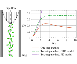
It is of considerable interest to compare the above results through the one-step GTD method to those produced by the two-step methods, including the GTD and PK models in previous studies (Hill & Bees Reference Hill and Bees2002; Bearon et al. Reference Bearon, Bees and Croze2012). The two-step GTD method requires that the swimming Péclet number  $\mathit{Pe}_{s}$ should be sufficiently small in order to avoid the influence of the reflective boundary (Bearon et al. Reference Bearon, Hazel and Thorn2011). Additionally, the variation of shear rates relative to swimming should also be small because the convection–diffusion equation for the position space in the first step is approximated by the dispersion of swimming cells in an unbounded homogeneous shear flow. To measure the variation of the shear rates (quantified by
  $\unicode[STIX]{x2202}^{2}(\mathit{Pe}_{f}U)/\unicode[STIX]{x2202}r^{2}=-4\mathit{Pe}_{f}$ for the downwelling Poiseuille flow) relative to the swimming term (quantified by
  $\mathit{Pe}_{s}$) in the dimensionless conservation equation (2.13), we introduce the ratio between Péclet numbers,
 $$\begin{eqnarray}w_{V}\triangleq \frac{\mathit{Pe}_{f}}{\mathit{Pe}_{s}}=\frac{U_{m}^{\ast }}{V_{s}^{\ast }},\end{eqnarray}$$
 which is also the ratio of the mean flow speed to the swimming speed. We will show the discrepancy between the results of the one- and two-step methods in the  $\mathit{Pe}_{s}{-}w_{V}$ plane.
For the one-step GTD method, the Galerkin method with the reflection basis is applied to obtain the dispersion results. The series expansion is truncated up to  $n=40$ in the radial direction for the gyrotactic focusing and
  $l=10$ in the orientation space with spherical harmonics. The resulting Galerkin equation is solved.
For the two-step method, the mathematical structures of the GTD (Hill & Bees Reference Hill and Bees2002; Manela & Frankel Reference Manela and Frankel2003) and PK (Pedley & Kessler Reference Pedley and Kessler1990, Reference Pedley and Kessler1992) models are summarized by Bearon et al. (Reference Bearon, Bees and Croze2012) and Croze et al. (Reference Croze, Bearon and Bees2017). The parameters used in the GTD and PK models for C. nivalis with  $\unicode[STIX]{x1D706}=2.2$ can be found in appendix E of Bearon et al. (Reference Bearon, Bees and Croze2012). The overall drift and dispersivity are also evaluated by the GTD theory. Detailed calculations are based on Bees & Croze (Reference Bees and Croze2010, equations (6.1) and (6.2)); see also Croze et al. (Reference Croze, Bearon and Bees2017, equations (2.10) and (2.11)).
4.1 Local distribution  $P_{0}^{\infty }$

The long-time asymptotic state of the zeroth-order moment  $P_{0}^{\infty }$ is the steady marginal density function in the phase space
  $(r,\unicode[STIX]{x1D703},\unicode[STIX]{x1D719})$ (Ezhilan & Saintillan Reference Ezhilan and Saintillan2015; Jiang & Chen Reference Jiang and Chen2019a). As a local distribution, it can demonstrate the gyrotactic focusing and shear alignment of cells.
4.1.1 Distribution in phase space
Examples for the gyrotactic focusing of cells in vertical pipe flows are shown in figure 2. For the case of a downwelling flow, cells accumulate near the centre of the tube (Kessler Reference Kessler and Velarde1984, Reference Kessler1985), with the highest concentration at the centre  $(r=0)$. The distributions of cells in the
  $\unicode[STIX]{x1D719}{-}\unicode[STIX]{x1D703}$ plane at all the radial positions are similar: cells concentrate near the point
  $\unicode[STIX]{x1D719}=0$,
  $\unicode[STIX]{x1D703}=\unicode[STIX]{x03C0}/2$. Note that there is no obvious swimming bias towards the centre (
 $0<\unicode[STIX]{x1D719}<\unicode[STIX]{x03C0}$), which is significantly different from the biased distribution predicted by the FP equation in both the two-step methods (Bearon et al. Reference Bearon, Hazel and Thorn2011). For the upwelling flow, the results are just reversed: the concentration at the wall (
 $r=1$) is the highest (Kessler Reference Kessler and Velarde1984, Reference Kessler1985).

Figure 2. Density plot of local distributions  $P_{0}^{\infty }(r,\unicode[STIX]{x1D703},\unicode[STIX]{x1D719})$ of spherical and ellipsoidal gyrotactic cells at different radial positions: (a,d,g,j)
  $r=0$; (b,e,h,k)
  $r=0.5$; (c,f,i,l)
  $r=1$. (a–c) Spheres in downwelling flow (
 $\unicode[STIX]{x1D6FC}_{0}=0$); (d–f) ellipsoids in downwelling flow (
 $\unicode[STIX]{x1D6FC}_{0}=0.31$); (g–i) spheres in upwelling flow (
 $\unicode[STIX]{x1D6FC}_{0}=0$); (j–l) ellipsoids in upwelling flow (
 $\unicode[STIX]{x1D6FC}_{0}=0.31$). In all cases,
  $\unicode[STIX]{x1D706}=2.2$,
  $\mathit{Pe}_{s}=1$ and
  $w_{V}=1$.
The structure of the local distribution in the phase space can be captured by the dynamical system theory (Zöttl & Stark Reference Zöttl and Stark2012, Reference Zöttl and Stark2013; Santamaria et al. Reference Santamaria, De Lillo, Cencini and Boffetta2014). A local velocity field for the local transport problem in the phase space  $(r,\unicode[STIX]{x1D703},\unicode[STIX]{x1D719})$ can be defined as (Jiang & Chen Reference Jiang and Chen2019a)
 $$\begin{eqnarray}\boldsymbol{u}=(-\mathit{Pe}_{s}\sin \unicode[STIX]{x1D703}\sin \unicode[STIX]{x1D719},\dot{\unicode[STIX]{x1D703}},\dot{\unicode[STIX]{x1D719}}).\end{eqnarray}$$
 Swimmers will accumulate near stable critical points (with zero local velocity). For vertical downwelling pipe flow, the critical point  $(0,\unicode[STIX]{x03C0}/2,0)$ is stable, where cells swim perfectly upwards, resulting in gyrotactic focusing. In contrast, the critical point
  $(0,\unicode[STIX]{x03C0}/2,\unicode[STIX]{x03C0})$ is unstable, where cells swim downwards, resulting in an area with the lowest concentration. For the case of the upwelling flow, the cells accumulate near the reflective boundaries due to swinging motions towards the tube wall, similar to the trapping by tumbling motions near high-shear regions (Zöttl & Stark Reference Zöttl and Stark2013; Rusconi, Guasto & Stocker Reference Rusconi, Guasto and Stocker2014). Additionally, for the case of spherical cells without gyrotactic bias (
 $\unicode[STIX]{x1D6FC}_{0}=0$,
  $\unicode[STIX]{x1D706}=0$), note that the local velocity field is divergence-free, as shown in § A.2.1. Therefore, the local transport problem (3.30) with reflective boundary conditions (2.18) and (2.19) has a constant solution
  $P_{0}^{\infty }=1/(4\unicode[STIX]{x03C0}^{2})$. There is no stable critical point and thus no focusing. Note that the incident probability flux at the wall (
 $r=1,-\unicode[STIX]{x03C0}<\unicode[STIX]{x1D719}<0$) can be non-zero but is equal to the reflection flux (
 $0<\unicode[STIX]{x1D719}<\unicode[STIX]{x03C0}$) because the reflective boundary conditions (2.18) and (2.19) for the continuum transport equation (2.13) are a simplified description of the reflection process, assuming that the incidence and reflection of a cell happen in an instant.
For the influence of cell shape, as shown in figure 2(a,d) for the downwelling flow, the main difference between the cases of spheres ( $\unicode[STIX]{x1D6FC}_{0}=0$) and ellipsoids (
 $\unicode[STIX]{x1D6FC}_{0}=0.31$) is due to the effect of shear alignments. The concentrated area of ellipsoids in figure 2(d) is much smaller than that of spheres in figure 2(a) because the swimming direction of prolate cells is aligned closely along the streamlines of the flow by the strain effect. However, the focusing of ellipsoids in the radial direction is weaker than that of spheres. Shear alignments reduce the probability that prolate cells can swim towards the centre of the tube, resulting in a more uniform distribution in the radial direction. The discussion for the upwelling case is similar.
4.1.2 Orientation-space-mean probability density function
The gyrotactic focusing of cells near the centre of the tube can be illustrated more clearly in terms of the orientation-space-mean p.d.f.
 $$\begin{eqnarray}\langle P_{0}^{\infty }\rangle _{O}\triangleq \int _{0}^{\unicode[STIX]{x03C0}}\sin \unicode[STIX]{x1D703}\,\text{d}\unicode[STIX]{x1D703}\int _{0}^{2\unicode[STIX]{x03C0}}\text{d}\unicode[STIX]{x1D719}\,P_{0}^{\infty }(r,\unicode[STIX]{x1D703},\unicode[STIX]{x1D719}),\end{eqnarray}$$
 i.e. the marginal p.d.f. in the position plane  $r$–
$r$– $\unicode[STIX]{x1D713}$ (here independent of
  $\unicode[STIX]{x1D713}$). With the orientation space eliminated, results are compared to those by the two-step models for the transport problem in the position space (Bearon et al. Reference Bearon, Bees and Croze2012).
First, we discuss the case of the downwelling flow. As shown in figure 3, the gyrotactic focusing near the axis of the tube is enhanced with increased flow rates (also quantified by the ratio between speeds  $w_{V}$ with a fixed swimming speed). However, the distributions of the spherical cells in figure 3(a–c) are roughly the same. Namely, the focusing of spherical cells is nearly dependent only on
  $w_{V}$, the ratio between the Péclet numbers. Note that the steady gyrotactic focusing can be predicted by a Gaussian distribution (Kessler Reference Kessler and Velarde1984, Reference Kessler1985; Pedley & Kessler Reference Pedley and Kessler1992). Near the centre of the tube with sufficiently small shear, Bearon et al. (Reference Bearon, Bees and Croze2012) gave an asymptotic solution based on the two-step GTD method, in current notation,
 $$\begin{eqnarray}\langle P_{0}^{\infty }\rangle _{O}\sim \text{e}^{-\unicode[STIX]{x1D706}w_{V}r^{2}},\end{eqnarray}$$
 which depends only on  $w_{V}$ and
  $\unicode[STIX]{x1D706}$. We remark that this approximate result is hard to obtain directly from the local transport equation (3.30) in the whole phase space by asymptotic analysis, but can be simply derived from the effective transport equation only in the position space by the two-step method; see Bearon et al. (Reference Bearon, Bees and Croze2012, equation (24)). In the absence of gyrotactic bias (
 $\unicode[STIX]{x1D706}=0$), there is no focusing and the radial distribution is uniform.
For the influence of cell shape, shear alignments of ellipsoids ( $\unicode[STIX]{x1D6FC}_{0}=0.31$) can weaken the gyrotactic focusing, which is consistent with previous studies (Bearon et al. Reference Bearon, Hazel and Thorn2011; Croze et al. Reference Croze, Sardina, Ahmed, Bees and Brandt2013) for channel flows. Compared with the spherical case (
 $\unicode[STIX]{x1D6FC}_{0}=0$), distributions of ellipsoids are much more uniform in the radial direction. More importantly, the decrease of concentration near the centre of the tube from the spherical case to the ellipsoidal case is greater with both larger flow rates (quantified by
  $w_{V}$) and larger swimming Péclet numbers
  $\mathit{Pe}_{s}$, as shown in figure 3. The reason is that shear alignments by the strain effect can inhibit prolate cells from swimming towards the centre of the tube, as discussed in § 4.1.1. The increase of both
  $\mathit{Pe}_{s}$ and
  $w_{V}$ corresponds to a larger flow Péclet number
  $\mathit{Pe}_{f}$ due to the definition of
  $w_{V}$ (4.3), as the ratio between the Péclet numbers. Thus, the shear rate and the strain also increase, enhancing the inhibiting effect.

Figure 3. Orientation-space-mean p.d.f.s  $\langle P_{0}^{\infty }\rangle _{O}$ of cells in the downwelling flow for different swimming Péclet numbers
  $\mathit{Pe}_{s}$: (a,d,g)
  $\mathit{Pe}_{s}=0.1$; (b,e,h)
  $\mathit{Pe}_{s}=1$; (c,f,i)
  $\mathit{Pe}_{s}=10$; and different ratios between speeds
  $w_{V}$: (a–c)
  $w_{V}=0.1$; (d–f)
  $w_{V}=1$; (g–i)
  $w_{V}=10$. ‘Spherical’ denotes the case of gyrotactic spherical cells (
 $\unicode[STIX]{x1D6FC}_{0}=0$,
  $\unicode[STIX]{x1D706}=2.2$). ‘Ellipsoidal’ denotes ellipsoidal cells (
 $\unicode[STIX]{x1D6FC}_{0}=0.31$,
  $\unicode[STIX]{x1D706}=2.2$). ‘No gyrotaxis’ denotes spherical cells without gyrotactic bias (
 $\unicode[STIX]{x1D6FC}_{0}=0$,
  $\unicode[STIX]{x1D706}=0$). ‘Two-step, GTD’ and ‘Two-step, PK’ denote the results of spherical cells (
 $\unicode[STIX]{x1D6FC}_{0}=0$,
  $\unicode[STIX]{x1D706}=2.2$) by the two-step method with the GTD and PK models, respectively. ‘Asymptotic’ denotes the associated asymptotic Gaussian distribution (4.6).
For the case of spherical gyrotactic cells ( $\unicode[STIX]{x1D6FC}_{0}=0$,
  $\unicode[STIX]{x1D706}=2.2$), both the two-step method with the GTD model and that with the PK model (Bearon et al. Reference Bearon, Bees and Croze2012) give successful predictions with small swimming Péclet numbers
  $\mathit{Pe}_{s}$ and relative variations of shear rates of the Poiseuille flow (quantified by
  $w_{V}$). As confirmed in figure 3(a,b,d), these three curves are on top of each other. However, outside the required parameter range in the
  $\mathit{Pe}_{s}{-}w_{V}$ plane, as shown in figure 3(e,f,h,i), there are considerable differences of the results by the PK model from the exact results by the one-step method. With stronger shear, more uniform distributions are predicted in the PK model than in GTD models, due to neglecting the local spatial distribution (thus valid only for weak flows) (Bearon et al. Reference Bearon, Hazel and Thorn2011, Reference Bearon, Bees and Croze2012; Croze et al. Reference Croze, Bearon and Bees2017). On the other hand, the predictions given by the two-step GTD method are still in agreement with the exact results, even in figure 3(i) with large
  $\mathit{Pe}_{s}$ and
  $w_{V}$. To some extent, the gyrotactic focusing accumulates cells in the regions with low shear and far from the tube wall, which enlarges the appropriate parameter range for the two-step method (Bearon et al. Reference Bearon, Hazel and Thorn2011).

Figure 4. Orientation-space-mean p.d.f.s  $\langle P_{0}^{\infty }\rangle _{O}$ of cells in the upwelling flow for different swimming Péclet numbers
  $\mathit{Pe}_{s}$: (a,d,g)
  $\mathit{Pe}_{s}=0.1$; (b,e,h)
  $\mathit{Pe}_{s}=1$; (c,f,i)
  $\mathit{Pe}_{s}=10$; and different ratios between speeds
  $w_{V}$: (a–c)
  $w_{V}=0.1$; (d–f)
  $w_{V}=1$; (g–i)
  $w_{V}=10$. ‘Spherical’ denotes the case of gyrotactic spherical cells (
 $\unicode[STIX]{x1D6FC}_{0}=0$,
  $\unicode[STIX]{x1D706}=2.2$). ‘Ellipsoidal’ denotes ellipsoidal cells (
 $\unicode[STIX]{x1D6FC}_{0}=0.31$,
  $\unicode[STIX]{x1D706}=2.2$). ‘No gyrotaxis’ denotes spherical cells without gyrotactic bias (
 $\unicode[STIX]{x1D6FC}_{0}=0$,
  $\unicode[STIX]{x1D706}=0$). ‘Two-step, GTD’ and ‘Two-step, PK’ denote the results for spherical cells (
 $\unicode[STIX]{x1D6FC}_{0}=0$,
  $\unicode[STIX]{x1D706}=2.2$) by the two-step method with the GTD and PK models, respectively. ‘Asymptotic’ denotes the associated asymptotic Gaussian distribution (4.6) with
  $\unicode[STIX]{x1D706}=-2.2$.
Now we turn to the case of the upwelling flow. The distinct difference is that the gyrotactic focusing is near the walls (Kessler Reference Kessler and Velarde1984, Reference Kessler1985), as shown in figure 4. As in the upwelling case, the orientation-space-mean p.d.f. can still be matched by the asymptotic solution (4.6) with the reversed sign of shear, although the shear near the wall is much larger than that near the centre of the tube. When the shear rate is large, shown in figure 4(g–i), the focusing is so intense that higher-order basis functions in the radial direction are needed for the series expansion (3.27) to reduce the truncation error. Also, distributions of spherical cells are nearly independent of swimming Péclet number  $\mathit{Pe}_{s}$ with a fixed ratio between speeds
  $w_{V}$, but it is not true for the ellipsoids. The shear alignments can also flatten the distributions in the radial direction. The discussion about the predictions by the two-step methods is analogous: the GTD model gives more successful results than the PK model, even inside the ‘breakdown’ parameter region.
4.2 Overall drift and dispersivity for downwelling flow
For the downwelling flow, the gyrotactic focusing near the centre of the tube, as demonstrated by the local distribution, will exert a strong influence on the overall dispersion process in the longitudinal direction. Results of the overall drift and dispersivity in the parameter plane  $\mathit{Pe}_{s}{-}w_{V}$ are presented. Here, we focus on the effects of shear and boundaries on the dispersion coefficients. The influence of cell shape and the predictions by the two-step methods will be tested.
4.2.1 Influence of shear flow
First, we discuss the influence of shear on the overall drift of spherical cells. Note that  $U_{d}$ (3.34) is the drift above the mean flow because the frame of reference has been transformed in (2.11). With the swimming Péclet number
  $\mathit{Pe}_{s}$ fixed, changing the ratio between speeds
  $w_{V}$ in figure 5 corresponds to changing the flow rate and shear rate.
The drift increases monotonically with the flow rate, as shown in figure 5(a,c,e). At small flow rates, where the swimming effect is dominant, the drift is negative due to the upward orientation of the cells by the gravitational torque (Bees & Croze Reference Bees and Croze2010; Croze et al. Reference Croze, Bearon and Bees2017). As the flow rate increases, the drift becomes positive because the gyrotactic focusing accumulates cells near the centre of the tube where the flow speed  $\mathit{Pe}_{f}$ is the fastest. Therefore, at high flow rates, it is observed that
  $U_{d}\sim \mathit{Pe}_{f}=w_{V}\mathit{Pe}_{s}$, which is consistent with the discussion by Croze et al. (Reference Croze, Bearon and Bees2017). In the absence of gyrotactic bias (
 $\unicode[STIX]{x1D706}=0$), there is no drift above the mean flow because the local distribution is uniform in the whole phase space.
Next, for the dispersivity, its variation with flow rate is much more complex. Note that the dispersion process is driven by both the swimming diffusion effect and the convection (Jiang & Chen Reference Jiang and Chen2019a). When the swimming Péclet number  $\mathit{Pe}_{s}$ is not large, the convection effect plays the central role. As shown in figure 5(b,d), the dispersivity rises as the flow rate increases. However, at high flow rates, the dispersivity appears to ‘saturate’ and then falls with
  $w_{V}$ (Croze et al. Reference Croze, Sardina, Ahmed, Bees and Brandt2013, Reference Croze, Bearon and Bees2017). The reason is that the gyrotactic focusing of cells near the centre of the tube greatly hinders the effect of convection on the dispersion process. Therefore, without gyrotactic bias (
 $\unicode[STIX]{x1D706}=0$), the dispersivity increases monotonically with the flow rate and is much larger than that of gyrotactic cells.
When the swimming Péclet number  $\mathit{Pe}_{s}$ is large, the strong swimming diffusion drives the macrotransport process. As shown in figure 5(f), there are significant differences in the trends of dispersivity with flow rates compared with those in figure 5(b,d): the dispersivity will first decrease, then it increases and saturates like the convection-effect-dominated cases. More importantly, in the absence of gyrotaxis, there is also a sharp decrease in dispersivity before the rising. Namely, the imposed shear can reduce the swimming diffusion effect. To find the reason, note that the swimming diffusion effect can be quantified by
  $V_{s}^{2}/D_{r}$ (Bearon et al. Reference Bearon, Hazel and Thorn2011). The imposed shear will enhance the rotation of cells, and thus reduce the swimming range, resulting in the decrease of the dispersivity.
Additionally, gyrotaxis can also reduce the swimming diffusion effect. As shown in figure 5(d,f) at small flow rates, i.e. the swimming-effect-dominated region, it results in a much smaller dispersivity compared with the no-bias case. Because gyrotaxis forces cells to swim upwards together, the tendency of the cells to separate from each other by swimming with rotation diffusion is weakened. However, the perfectly upward orientation of cells can be disturbed by the imposed shear due to the enhanced rotation, resulting in an increase in dispersivity, in contrast to the decrease discussed above. In fact, these enhanced and reduced effects of the shear rotation on the dispersion process will be balanced: the dispersivity of the gyrotactic case is comparable to that without the bias, as shown in figure 5(b) when  $w_{V}<2$.

Figure 5. For the downwelling flow, variations of (a,c,e) overall drift  $U_{d}$ (3.34) and (b,d,f) dispersivity
  $D_{T}$ (3.35) with the ratio between speeds
  $w_{V}$ subject to different fixed swimming Péclet numbers
  $\mathit{Pe}_{s}$: (a,b)
  $\mathit{Pe}_{s}=0.1$; (c,d)
  $\mathit{Pe}_{s}=1$; (e,f)
  $\mathit{Pe}_{s}=10$. ‘Spherical’ denotes the case of gyrotactic spherical cells (
 $\unicode[STIX]{x1D6FC}_{0}=0$,
  $\unicode[STIX]{x1D706}=2.2$). ‘Ellipsoidal’ denotes ellipsoidal cells (
 $\unicode[STIX]{x1D6FC}_{0}=0.31$,
  $\unicode[STIX]{x1D706}=2.2$). ‘No gyrotaxis’ denotes spherical cells without gyrotactic bias (
 $\unicode[STIX]{x1D6FC}_{0}=0$,
  $\unicode[STIX]{x1D706}=0$). ‘Two-step, GTD’ and ‘Two-step, PK’ denote the results for spherical cells (
 $\unicode[STIX]{x1D6FC}_{0}=0$,
  $\unicode[STIX]{x1D706}=2.2$) by the two-step method with the GTD and PK models, respectively. Note that with
  $\mathit{Pe}_{s}$ fixed, increasing
  $w_{V}$ corresponds to increasing the mean speed
  $U_{m}^{\ast }$.
With respect to the influence of cell shape, shear alignments of ellipsoids ( $\unicode[STIX]{x1D6FC}_{0}=0.31$) can slightly reduce the drift and greatly enhance the dispersivity, because the gyrotactic focusing is weakened (Croze et al. Reference Croze, Sardina, Ahmed, Bees and Brandt2013). As discussed in § 4.1.1, the local distribution of ellipsoids is more uniform in the radial direction, compared with that of spheres. Therefore, more cells swim outside the fast flow zone, decreasing the drift above the mean flow. Meanwhile, the convection effect on the dispersion process is strengthened.
The predictions by the two-step methods on the dispersion process are compared with the results by the one-step method for the case of spherical gyrotactic cells. When the swimming Péclet number  $\mathit{Pe}_{s}$ is small, as required in the two-step methods, both the GTD and PK models provide perfect results for the drift and dispersivity as expected, also shown in figure 5(a,b), although there is still a small deviation in dispersivity at high flow rates (quantified by
  $w_{V}$). With larger
  $\mathit{Pe}_{s}$, considerable discrepancies are observed in figure 5(c–f). Instead of growing with the flow rate, the drift by the PK model tends to be a constant much smaller than the exact one at high flow rates (Croze et al. Reference Croze, Sardina, Ahmed, Bees and Brandt2013, Reference Croze, Bearon and Bees2017). As discussed in § 4.1.1, the PK model neglects the local spatial distribution by shear and predicts a more uniform distribution of cells in the radial direction, resulting in a smaller drift similar to the case without gyrotactic bias. In the GTD model, the curve of drift still adheres to the exact one, but curves of dispersivity diverge. The deviation in dispersivity becomes larger as the variation of shear rates in the radial direction (also quantified by the ratio between Péclet numbers
  $w_{V}$ for the Poiseuille flow) increases and exceeds the requirements of the first step in obtaining the convection–diffusion equation in the position space.
4.2.2 Influence of boundaries
We have tested the predictions produced by the two-step methods on the dispersion process with the variation of shear rates  $w_{V}$ at different swimming Péclet numbers
  $\mathit{Pe}_{s}$. Here, we give a more direct illustration of the influence of
  $\mathit{Pe}_{s}$, with
  $w_{V}$ fixed. Note that for C. nivalis with fixed swimming velocity
  $V_{s}^{\ast }$ and rotational diffusivity
  $D_{r}^{\ast }$, increasing
  $\mathit{Pe}_{s}$ corresponds to decreasing the pipe radius
  $a^{\ast }$, and thus increasing the influence of boundaries.
Changing  $\mathit{Pe}_{s}$ hardly affects the gyrotactic focusing, as discussed in § 4.1.1. However, it significantly influences the drift and dispersivity as functions of
  $w_{V}$, as shown in figure 5. With a fixed ratio between Péclet numbers
  $w_{V}$, i.e. the relative importance of the shear effect to the swimming effect, increasing
  $\mathit{Pe}_{s}$ will enhance both these effects. Therefore, the drift and dispersivity vary monotonically with
  $\mathit{Pe}_{s}$, for both cases of spherical and ellipsoidal cells, as shown in figure 6.
To obtain the convection–diffusion equation in the position space in the two-step methods, a small  $\mathit{Pe}_{s}$ is the key requirement, which means that the influence of boundaries can be neglected (Bearon et al. Reference Bearon, Hazel and Thorn2011). As shown in figure 6, increasing
  $\mathit{Pe}_{s}$ is destructive to the validity of the two-step methods, for both PK and GTD models. The discrepancies in the drift and dispersivity between the two-step methods and the exact ones grow considerably with
  $\mathit{Pe}_{s}$. Note that, although the reflective boundary conditions (2.18) and (2.19) considered in the current study are an idealized condition for the population models, it is demonstrated that the existence of boundaries will lead to significant deviations in the two-step methods. In fact, when boundaries play a central role, more complicated effects, e.g. hydrodynamic interactions between cells and walls (Berke et al. Reference Berke, Turner, Berg and Lauga2008), should be taken into consideration in both the one-step and two-step methods for the dispersion process.

Figure 6. For downwelling flow, variations of (a,c,e) overall drift  $U_{d}$ (3.34) and (b,d,f) dispersivity
  $D_{T}$ (3.35) with the swimming Péclet number
  $\mathit{Pe}_{s}$ subject to different fixed relative variations of shear rates (quantified by the ratio between Péclet numbers
  $w_{V}$): (a,b)
  $w_{V}=0.1$; (c,d)
  $w_{V}=1$; (e,f)
  $w_{V}=10$. ‘Spherical’ denotes the case of gyrotactic spherical cells (
 $\unicode[STIX]{x1D6FC}_{0}=0$,
  $\unicode[STIX]{x1D706}=2.2$). ‘Ellipsoidal’ denotes ellipsoidal cells (
 $\unicode[STIX]{x1D6FC}_{0}=0.31$,
  $\unicode[STIX]{x1D706}=2.2$). ‘No gyrotaxis’ denotes spherical cells without gyrotactic bias (
 $\unicode[STIX]{x1D6FC}_{0}=0$,
  $\unicode[STIX]{x1D706}=0$). ‘Two-step, GTD’ and ‘Two-step, PK’ denote the results of spherical cells (
 $\unicode[STIX]{x1D6FC}_{0}=0$,
  $\unicode[STIX]{x1D706}=2.2$) by the two-step method with the GTD and PK models, respectively. Note that for the studied case, increasing
  $\mathit{Pe}_{s}$ corresponds to decreasing the pipe radius
  $a^{\ast }$.
4.3 Overall drift and dispersivity for upwelling flow
For the upwelling flow, the position of the gyrotactic focusing is reversed from the centre to the wall of the tube. However, the results of the overall drift and dispersivity are similar to those of the downwelling flow. We keep all the parameters the same as those of the downwelling case and give an analogous discussion on the influence of shear flow.
As in the downwelling case, the drift is monotonic with the flow rate, as shown in figure 7(a,c,e). Note that the drift  $U_{d}$ (3.34) is above the mean flow; thus changing the direction of the flow does not affect the trend of cells towards the mean flow. The explanation for the change of the sign of the drift is similar to those for the downwelling case (Croze et al. Reference Croze, Sardina, Ahmed, Bees and Brandt2013). At high flow rates, the gyrotactic focusing is near the wall, where the flow rate is also positive to the mean flow, resulting in the positive drift.

Figure 7. For the upwelling flow, variations of (a,c,e) overall drift  $U_{d}$ (3.34) and (b,d,f) dispersivity
  $D_{T}$ (3.35) with the ratio between speeds
  $w_{V}$ subject to different fixed swimming Péclet numbers
  $\mathit{Pe}_{s}$: (a,b)
  $\mathit{Pe}_{s}=0.1$; (c,d)
  $\mathit{Pe}_{s}=1$; (e,f)
  $\mathit{Pe}_{s}=10$. ‘Spherical’ denotes the case of gyrotactic spherical cells (
 $\unicode[STIX]{x1D6FC}_{0}=0$,
  $\unicode[STIX]{x1D706}=2.2$). ‘Ellipsoidal’ denotes ellipsoidal cells (
 $\unicode[STIX]{x1D6FC}_{0}=0.31$,
  $\unicode[STIX]{x1D706}=2.2$). ‘No gyrotaxis’ denotes spherical cells without gyrotactic bias (
 $\unicode[STIX]{x1D6FC}_{0}=0$,
  $\unicode[STIX]{x1D706}=0$). ‘Two-step, GTD’ and ‘Two-step, PK’ denote the results for spherical cells (
 $\unicode[STIX]{x1D6FC}_{0}=0$,
  $\unicode[STIX]{x1D706}=2.2$) by the two-step method with the GTD and PK models, respectively.
For the dispersivity, as shown in figure 7(b,d,f), trends with flow rates are similar to those of the downwelling case: the dispersivity rises and then falls with the ratio between speeds  $w_{V}$. Also, there is a slight decrease at low flow rates when the swimming Péclet number
  $\mathit{Pe}_{s}$ is large. The explanation for gyrotaxis reducing both the convection and the swimming diffusion effects is analogous. However, the changed position of the focusing from the centre to the wall does have an influence on the dispersion process: the dispersivity is significantly smaller, comparing figure 7(b,d) with figure 5(b,d). This can be understood by the orientation-space-mean p.d.f.s: the distribution of the upwelling case is not as uniform as the downwelling case. Therefore, the convection effect on the dispersion process is weakened. On the other hand, when the swimming diffusion effect is dominant, as shown in figure 7(f) and figure 5(f), the dispersivity of the upwelling case is larger. Note that, due to the focusing, the characteristic length for the dispersion process is smaller than the radius of the tube, namely, a larger effective swimming Péclet number can be defined similarly to
  $\mathit{Pe}_{s}$ as in (2.11). For the upwelling case with a steeper distribution in the radial direction, the effective swimming Péclet number is larger than that of the downwelling case, resulting in the stronger swimming diffusion effect.
For the ellipsoidal swimmers, the influence of shear alignments on the dispersion process is similar to the downwelling case: the drift is reduced and the dispersivity is enhanced, because of the stronger convection effect under a more uniform radial distribution. However, when the swimming diffusion effect is strong, as shown in figure 7(f), the dispersivity is comparable to the downwelling one. This is also because of the changed position of the focusing. As discussed above, the swimming diffusion effect is weakened due to the more uniform distribution; thus it cancels out the enhancement by the convection effect.
The predictions by the two-step methods for the upwelling case are also tested. For the overall drift as shown in figure 7(a,c,e), the GTD model gives more successful results than the PK model. However, for the dispersivity, both these two-step methods fail in their ‘breakdown’ parameter region, as shown in figure 7(d,f). The reason is similar to the downwelling case: their restrictions on the derivation of the convective–diffusion equation in the position space during the first step. Additionally, the discussion on the influence of boundaries is also similar. As shown in figure 8, the discrepancies in the drift and dispersivity between the two- and one-step methods grow considerably with the swimming Péclet number  $\mathit{Pe}_{s}$.

Figure 8. For the upwelling flow, variations of (a,c,e) overall drift  $U_{d}$ (3.34) and (b,d,f) dispersivity
  $D_{T}$ (3.35) with the swimming Péclet number
  $\mathit{Pe}_{s}$ subject to different fixed relative variations of shear rates (quantified by the ratio between Péclet numbers
  $w_{V}$): (a,b)
  $w_{V}=0.1$; (c,d)
  $w_{V}=1$; (e,f)
  $w_{V}=10$. ‘Spherical’ denotes the case of gyrotactic spherical cells (
 $\unicode[STIX]{x1D6FC}_{0}=0$,
  $\unicode[STIX]{x1D706}=2.2$). ‘Ellipsoidal’ denotes ellipsoidal cells (
 $\unicode[STIX]{x1D6FC}_{0}=0.31$,
  $\unicode[STIX]{x1D706}=2.2$). ‘No gyrotaxis’ denotes spherical cells without gyrotactic bias (
 $\unicode[STIX]{x1D6FC}_{0}=0$,
  $\unicode[STIX]{x1D706}=0$). ‘Two-step, GTD’ and ‘Two-step, PK’ denote the results of spherical cells (
 $\unicode[STIX]{x1D6FC}_{0}=0$,
  $\unicode[STIX]{x1D706}=2.2$) by the two-step method with the GTD and PK models, respectively.
5 Conclusions
For dispersion of dilute suspensions of gyrotactic micro-organisms in vertical pipe flows, previous work used the two-step methods with the PK model and GTD model and obtained only approximate values of the overall drift and dispersivity. This study provides the first analytical derivation for the dispersion coefficients, by the integrated one-step GTD method. Prior to this study, it was difficult to analyse the dispersion process in the ‘breakdown’ parameter region in the two-step methods due to the restrictive assumptions: both the swimming Péclet number and the variation of shear rates relative to swimming must be sufficiently small. Thus, the results also give a quantitative test for the applicability of the two-step methods, which is of considerable interest.
Another strength of this study is proposing an appropriate function basis under reflective boundary conditions for the series expansion in the Galerkin method. The reflection principle used in previous studies does not apply to the current flow case, because one cannot reflect the pipe flow field on the circular cross-section. Instead, the required basis functions are constructed by cylindrical and spherical harmonics, using the full form of reflective boundary conditions (2.18) and (2.19), including both the probability and its radial derivative. The so-called reflection basis plays the central role in solving the local distribution, the overall drift and the dispersivity in the one-step GTD method.
Detailed results for C. nivalis are presented to illustrate the influence of the gyrotactic focusing on the overall dispersion process, for both the downwelling and upwelling flows. The gyrotactic bias is demonstrated by the local distribution in the phase space. The drift above the mean flow increases monotonically with the flow rate. For the dispersivity, when the flow rate is small, the combined effect of gyrotaxis, swimming and shear on the dispersion process is complicated: the dispersivity first decreases, then increases and finally saturates as the flow rate increases. For prolate cells, shear alignments with streamlines of the imposed flow lead to weaker focusing than that of spherical ones, and thus reduce the overall drift and greatly enhance the overall dispersivity. For the case of spherical gyrotactic cells, the predictions by the two-step methods are compared with the exact results. Both the PK and GTD models give successful predictions inside their required parameter region. Within the ‘breakdown’ region, the predictions of the two-step GTD method are still matched for the local distribution and the overall drift, but fail in the overall dispersivity.
This study has only considered dilute suspensions, and idealized reflective boundary conditions are imposed for the theoretical analysis. Future studies should include cell–cell, cell–fluid and cell–wall interactions in the one-step approach for dense suspensions. The challenge is to solve the Smoluchowski equation for transport coupled to the Navier–Stokes equation as modified by adding a new term to reflect the active stress in the flow field (Bees & Croze Reference Bees and Croze2010; Croze et al. Reference Croze, Bearon and Bees2017; Saintillan Reference Saintillan2018). Self-organization (Lushi, Wioland & Goldstein Reference Lushi, Wioland and Goldstein2014) and hydrodynamic instabilities (Pedley & Kessler Reference Pedley and Kessler1992; Hwang & Pedley Reference Hwang and Pedley2014b) should also be considered in finding the local distribution. Additionally, the dispersion process can be very sensitive to the type of boundary conditions. For example, the Robin boundary condition (Ezhilan & Saintillan Reference Ezhilan and Saintillan2015) accounting for the wall accumulation effect of micro-organisms like bacteria and sperms can enhance or reduce the overall dispersivity compared with those under the reflective boundary condition (Jiang & Chen Reference Jiang and Chen2019a). In fact, the experimentally observed behaviour of swimming micro-organisms at boundaries can be much more complicated (Bianchi, Saglimbeni & Di Leonardo Reference Bianchi, Saglimbeni and Di Leonardo2017; Lushi, Kantsler & Goldstein Reference Lushi, Kantsler and Goldstein2017). Further work is required to develop appropriate boundary conditions for the continuum transport model to characterize the complex cell–wall interactions such as sliding, scattering and steric repulsion effects (Drescher et al. Reference Drescher, Dunkel, Cisneros, Ganguly and Goldstein2011; Kantsler et al. Reference Kantsler, Dunkel, Polin and Goldstein2013; Contino et al. Reference Contino, Lushi, Tuval, Kantsler and Polin2015).
Acknowledgements
This work is supported by the National Natural Science Foundation of China (grant no. 51879002).
Declaration of interests
The authors report no conflict of interest.
Appendix A. Galerkin method with spherical harmonics
The idea of systemically treating spherical harmonics in the Galerkin method was given by Doi & Edwards (Reference Doi and Edwards1978). The key is to express the local operator  ${\mathcal{L}}$ in terms of the angular momentum operators and multiplication operators with spherical harmonics. Here we reveal their relation generally.
A.1 Angular momentum operators
In quantum mechanics, the orbital angular momentum operator is defined as (Doi & Edwards Reference Doi and Edwards1978)
 $$\begin{eqnarray}\boldsymbol{L}\triangleq -\text{i}\hbar (\boldsymbol{r}\times \unicode[STIX]{x1D735}),\end{eqnarray}$$
 where  $\hbar$ is the Planck constant and
  $\boldsymbol{r}$ is the position vector. Its three components
  $(L_{x},L_{y},L_{z})$ in Cartesian coordinates can be expressed in terms of spherical coordinates as
 $$\begin{eqnarray}\displaystyle & \displaystyle L_{x}=-\text{i}\hbar \left(-\sin \unicode[STIX]{x1D719}\frac{\unicode[STIX]{x2202}}{\unicode[STIX]{x2202}\unicode[STIX]{x1D703}}-\cot \unicode[STIX]{x1D703}\cos \unicode[STIX]{x1D719}\frac{\unicode[STIX]{x2202}}{\unicode[STIX]{x2202}\unicode[STIX]{x1D719}}\right), & \displaystyle\end{eqnarray}$$
 $$\begin{eqnarray}\displaystyle & \displaystyle L_{y}=-\text{i}\hbar \left(\cos \unicode[STIX]{x1D719}\frac{\unicode[STIX]{x2202}}{\unicode[STIX]{x2202}\unicode[STIX]{x1D703}}-\cot \unicode[STIX]{x1D703}\sin \unicode[STIX]{x1D719}\frac{\unicode[STIX]{x2202}}{\unicode[STIX]{x2202}\unicode[STIX]{x1D719}}\right), & \displaystyle\end{eqnarray}$$
 $$\begin{eqnarray}\displaystyle & \displaystyle L_{z}=-\text{i}\hbar \frac{\unicode[STIX]{x2202}}{\unicode[STIX]{x2202}\unicode[STIX]{x1D719}}. & \displaystyle\end{eqnarray}$$
 The square of  $\boldsymbol{L}$,
 $$\begin{eqnarray}\boldsymbol{L}^{2}=\boldsymbol{L}\boldsymbol{\cdot }\boldsymbol{L}=L_{x}^{2}+L_{y}^{2}+L_{z}^{2},\end{eqnarray}$$
gives the Laplace operator, and in spherical coordinates
 $$\begin{eqnarray}\boldsymbol{L}^{2}=-\hbar ^{2}\left[\frac{1}{\sin \unicode[STIX]{x1D703}}\frac{\unicode[STIX]{x2202}}{\unicode[STIX]{x2202}\unicode[STIX]{x1D703}}\left(\sin \unicode[STIX]{x1D703}\frac{\unicode[STIX]{x2202}}{\unicode[STIX]{x2202}\unicode[STIX]{x1D703}}\right)+\frac{1}{\sin ^{2}\unicode[STIX]{x1D703}}\frac{\unicode[STIX]{x2202}^{2}}{\unicode[STIX]{x2202}\unicode[STIX]{x1D719}^{2}}\right].\end{eqnarray}$$
Note that the results of the angular momentum operator on spherical harmonics are simple. To illustrate, the spherical harmonics (3.9), (3.10) and (3.11) are redefined with complex exponentials
 $$\begin{eqnarray}\text{Y}_{l}^{m}(\unicode[STIX]{x1D703},\unicode[STIX]{x1D719})=\sqrt{\frac{2l+1}{4\unicode[STIX]{x03C0}}\frac{(l-m)!}{(l+m)!}}\,\text{P}_{l}^{m}(\cos \unicode[STIX]{x1D703})\text{e}^{\text{i}m\unicode[STIX]{x1D719}},\end{eqnarray}$$
 where  $m=-l,-(l-1),\ldots ,0,\ldots ,l-1$. The orthogonality relationship is
 $$\begin{eqnarray}\int _{0}^{2\unicode[STIX]{x03C0}}\text{d}\unicode[STIX]{x1D719}\int _{0}^{\unicode[STIX]{x03C0}}\overline{\text{Y}_{l^{\prime }}^{m^{\prime }}}(\unicode[STIX]{x1D703},\unicode[STIX]{x1D719})\text{Y}_{l}^{m}(\unicode[STIX]{x1D703},\unicode[STIX]{x1D719})\sin \unicode[STIX]{x1D703}\,\text{d}\unicode[STIX]{x1D703}=\unicode[STIX]{x1D6FF}_{ll^{\prime }}\unicode[STIX]{x1D6FF}_{mm^{\prime }},\end{eqnarray}$$
 where the bar denotes the complex conjugate. For  $L_{z}$ on spherical harmonics,
 $$\begin{eqnarray}L_{z}\text{Y}_{l}^{m}(\unicode[STIX]{x1D703},\unicode[STIX]{x1D719})=m\hbar \text{Y}_{l}^{m}(\unicode[STIX]{x1D703},\unicode[STIX]{x1D719}).\end{eqnarray}$$
 For components  $L_{x}$ and
  $L_{y}$, one can introduce the ladder operators (Doi & Edwards Reference Doi and Edwards1978)
 $$\begin{eqnarray}L_{\pm }\triangleq L_{x}\pm \text{i}L_{y},\end{eqnarray}$$
which have the following important property:
 $$\begin{eqnarray}L_{\pm }\text{Y}_{l}^{m}(\unicode[STIX]{x1D703},\unicode[STIX]{x1D719})=\hbar [l(l+1)-m(m\pm 1)]^{1/2}\text{Y}_{l}^{m\pm 1}(\unicode[STIX]{x1D703},\unicode[STIX]{x1D719}).\end{eqnarray}$$
Therefore, one can use
 $$\begin{eqnarray}\displaystyle & \displaystyle L_{x}={\textstyle \frac{1}{2}}(L_{+}+L_{-}), & \displaystyle\end{eqnarray}$$
 $$\begin{eqnarray}\displaystyle & \displaystyle L_{y}=-\text{i}{\textstyle \frac{1}{2}}(L_{+}-L_{-}), & \displaystyle\end{eqnarray}$$
to obtain the results of their action on spherical harmonics.
A.2 Expression of local operator by angular momentum operators
In the swimming orientation space, the local operator  ${\mathcal{L}}$ can be expressed in terms of the angular momentum operator
  $\boldsymbol{L}$. The main part of
  ${\mathcal{L}}$ (3.2) that needs treating is
 $$\begin{eqnarray}{\mathcal{L}}_{p}f\triangleq \unicode[STIX]{x1D735}_{p}\boldsymbol{\cdot }(\dot{\boldsymbol{p}_{r}}f),\end{eqnarray}$$
because
 $$\begin{eqnarray}\unicode[STIX]{x1D735}_{p}\boldsymbol{\cdot }\unicode[STIX]{x1D735}_{p}=\unicode[STIX]{x1D6E5}_{p}=-\frac{\boldsymbol{L}^{2}}{\hbar ^{2}}\end{eqnarray}$$
is just the Laplace operator in the orientation space and the radial convective term in (3.30) can be written as
 $$\begin{eqnarray}\displaystyle -\mathit{Pe}_{s}\sin \unicode[STIX]{x1D703}\sin \unicode[STIX]{x1D719}\frac{1}{r}\frac{\unicode[STIX]{x2202}(rf)}{\unicode[STIX]{x2202}r} & = & \displaystyle -\mathit{Pe}_{s}\sin \unicode[STIX]{x1D703}\sin \unicode[STIX]{x1D719}\left(\frac{f}{r}+\frac{\unicode[STIX]{x2202}f}{\unicode[STIX]{x2202}r}\right)\nonumber\\ \displaystyle & = & \displaystyle -\,\mathit{Pe}_{s}\text{i}\sqrt{\frac{2\unicode[STIX]{x03C0}}{3}}[\text{Y}_{1}^{-1}(\unicode[STIX]{x1D703},\unicode[STIX]{x1D711})+\text{Y}_{1}^{1}(\unicode[STIX]{x1D703},\unicode[STIX]{x1D711})]\left(\frac{f}{r}+\frac{\unicode[STIX]{x2202}f}{\unicode[STIX]{x2202}r}\right).\qquad\end{eqnarray}$$
 Note that according to (2.4) and (2.14),  ${\mathcal{L}}_{p}$ (A 14) can be rewritten as
 $$\begin{eqnarray}{\mathcal{L}}_{p}f=\unicode[STIX]{x1D735}_{p}\boldsymbol{\cdot }\left[\left(\unicode[STIX]{x1D734}_{r}\times \boldsymbol{p}\right)f\right],\end{eqnarray}$$
 where  $\unicode[STIX]{x1D734}_{r}$ is the dimensionless relative angular velocity,
 $$\begin{eqnarray}\displaystyle \unicode[STIX]{x1D734}_{r} & = & \displaystyle \unicode[STIX]{x1D734}_{a}-\dot{\unicode[STIX]{x1D713}}\boldsymbol{e}_{z}\nonumber\\ \displaystyle & = & \displaystyle \unicode[STIX]{x1D706}\boldsymbol{p}\times \boldsymbol{k}+\frac{1}{2}\mathit{Pe}_{f}\unicode[STIX]{x1D74E}+\unicode[STIX]{x1D6FC}_{0}\mathit{Pe}_{f}[\boldsymbol{p}\times (\unicode[STIX]{x1D640}\boldsymbol{\cdot }\boldsymbol{p})]-\frac{\mathit{Pe}_{s}\cos \unicode[STIX]{x1D703}}{r}\boldsymbol{e}_{z},\end{eqnarray}$$
 and the dimensionless total angular velocity is  $\unicode[STIX]{x1D734}_{a}\triangleq \unicode[STIX]{x1D734}_{a}^{\ast }/D_{r}^{\ast }$.
Next is to pass  ${\mathcal{L}}_{p}$ to the whole spherical coordinate system, i.e. the whole momentum space with the employed spherical coordinates
  $(\unicode[STIX]{x1D70C},\unicode[STIX]{x1D703},\unicode[STIX]{x1D719})$. At each point
  $(r,\unicode[STIX]{x1D713},z)$ of the position space, we also employ a Cartesian coordinate system for the momentum space, with
  $\hat{\boldsymbol{x}}=-\boldsymbol{e}_{z}$,
  $\hat{\boldsymbol{y}}=-\boldsymbol{e}_{r}$ and
  $\hat{\boldsymbol{z}}=\boldsymbol{e}_{\unicode[STIX]{x1D713}}$. To distinguish the gradient operator for the momentum space from
  $\unicode[STIX]{x1D735}_{p}$ on the unit sphere (orientation space), we use
  $\unicode[STIX]{x1D735}_{s}$ to denote it. Now the angular momentum operator (A 1) can be introduced to the momentum space as
 $$\begin{eqnarray}\displaystyle \boldsymbol{L} & = & \displaystyle -\text{i}\hbar (\unicode[STIX]{x1D746}\times \unicode[STIX]{x1D735}_{s})\nonumber\\ \displaystyle & = & \displaystyle L_{x}\hat{\boldsymbol{x}}+L_{y}\hat{\boldsymbol{y}}+L_{z}\hat{\boldsymbol{z}}\nonumber\\ \displaystyle & = & \displaystyle -L_{x}\boldsymbol{e}_{z}-L_{y}\boldsymbol{e}_{r}+L_{z}\boldsymbol{e}_{\unicode[STIX]{x1D713}},\end{eqnarray}$$
 where  $\unicode[STIX]{x1D746}=\unicode[STIX]{x1D70C}\boldsymbol{e}_{\unicode[STIX]{x1D70C}}=\unicode[STIX]{x1D70C}\boldsymbol{p}$ is the ‘position’ vector in the momentum space.
Note that operator  ${\mathcal{L}}_{p}$ (A 17) is independent of
  $\unicode[STIX]{x1D70C}$. Therefore, its results on the unit sphere (
 $\unicode[STIX]{x1D70C}=1$) in the momentum space are the same as those in the original orientation space:
 $$\begin{eqnarray}\displaystyle {\mathcal{L}}_{p}f & = & \displaystyle \unicode[STIX]{x1D735}_{s}\boldsymbol{\cdot }(\unicode[STIX]{x1D734}_{r}\times \boldsymbol{p}f)\nonumber\\ \displaystyle & = & \displaystyle (\unicode[STIX]{x1D735}_{s}\times \unicode[STIX]{x1D734}_{r})\boldsymbol{\cdot }\boldsymbol{p}f-\unicode[STIX]{x1D734}_{r}\boldsymbol{\cdot }[\unicode[STIX]{x1D735}_{s}\times (\boldsymbol{p}f)].\end{eqnarray}$$
 With  $\unicode[STIX]{x1D735}_{s}\times \boldsymbol{p}=0$, the second term of (A 20) can be expressed by the angular momentum operator (A 19)
 $$\begin{eqnarray}\displaystyle \unicode[STIX]{x1D735}_{s}\times (\boldsymbol{p}f) & = & \displaystyle -\boldsymbol{p}\times \unicode[STIX]{x1D735}_{s}f+(\unicode[STIX]{x1D735}_{s}\times \boldsymbol{p})f\nonumber\\ \displaystyle & = & \displaystyle \frac{\boldsymbol{L}}{\text{i}\hbar \unicode[STIX]{x1D70C}}f\nonumber\\ \displaystyle & = & \displaystyle \frac{\boldsymbol{L}}{\text{i}\hbar }f.\end{eqnarray}$$
Finally,
 $$\begin{eqnarray}{\mathcal{L}}_{p}f=(\unicode[STIX]{x1D735}_{s}\times \unicode[STIX]{x1D734}_{r})\boldsymbol{\cdot }\boldsymbol{p}f-\left(\unicode[STIX]{x1D734}_{r}\boldsymbol{\cdot }\frac{\boldsymbol{L}}{\text{i}\hbar }\right)f.\end{eqnarray}$$
 Note that this form of  ${\mathcal{L}}_{p}$ can also be obtained using the rotation operator (Brenner & Condiff Reference Brenner and Condiff1972).
A.2.1 Detailed expression for ${\mathcal{L}}_{p}$

We substitute  $\unicode[STIX]{x1D734}_{r}$ (A 18) into (A 22) to obtain the detailed expression for
  ${\mathcal{L}}_{p}$. The coefficients of
  ${\mathcal{L}}_{p}$ are replaced with corresponding spherical harmonics as multipliers for the bilinear form. In matrix form, the dimensionless relative angular velocity is
 $$\begin{eqnarray}\displaystyle \unicode[STIX]{x1D734}_{r} & = & \displaystyle \unicode[STIX]{x1D706}\left(\begin{array}{@{}c@{}}-\cos \unicode[STIX]{x1D703}\\ -\sin \unicode[STIX]{x1D703}\sin \unicode[STIX]{x1D719}\\ 0\end{array}\right)+\frac{\mathit{Pe}_{f}}{2}\frac{\unicode[STIX]{x2202}U}{\unicode[STIX]{x2202}r}\left(\begin{array}{@{}c@{}}0\\ -1\\ 0\end{array}\right)\nonumber\\ \displaystyle & & \displaystyle +\,\frac{\unicode[STIX]{x1D6FC}_{0}\mathit{Pe}_{f}}{2}\frac{\unicode[STIX]{x2202}U}{\unicode[STIX]{x2202}r}\left(\begin{array}{@{}c@{}}-\cos \unicode[STIX]{x1D703}\sin \unicode[STIX]{x1D703}\sin \unicode[STIX]{x1D719}\\ \sin ^{2}\unicode[STIX]{x1D703}\cos 2\unicode[STIX]{x1D719}\\ \cos \unicode[STIX]{x1D703}\sin \unicode[STIX]{x1D703}\cos \unicode[STIX]{x1D719}\end{array}\right)-\frac{\mathit{Pe}_{s}\cos \unicode[STIX]{x1D703}}{r}\left(\begin{array}{@{}c@{}}0\\ 0\\ 1\end{array}\right)\nonumber\\ \displaystyle & = & \displaystyle \unicode[STIX]{x1D706}\left(\begin{array}{@{}c@{}}-2\sqrt{{\displaystyle \frac{\unicode[STIX]{x03C0}}{3}}}\text{Y}_{1}^{0}\\ -\text{i}\sqrt{{\displaystyle \frac{2\unicode[STIX]{x03C0}}{3}}}(\text{Y}_{1}^{1}+\text{Y}_{1}^{-1})\\ 0\end{array}\right)+\frac{\mathit{Pe}_{f}}{2}\frac{\unicode[STIX]{x2202}U}{\unicode[STIX]{x2202}r}\left(\begin{array}{@{}c@{}}0\\ -1\\ 0\end{array}\right)\nonumber\\ \displaystyle & & \displaystyle +\,\frac{\unicode[STIX]{x1D6FC}_{0}\mathit{Pe}_{f}}{2}\frac{\unicode[STIX]{x2202}U}{\unicode[STIX]{x2202}r}\left(\begin{array}{@{}c@{}}-\text{i}\sqrt{{\displaystyle \frac{2\unicode[STIX]{x03C0}}{15}}}(\text{Y}_{2}^{1}+\text{Y}_{2}^{-1})\\ 2\sqrt{{\displaystyle \frac{2\unicode[STIX]{x03C0}}{15}}}(\text{Y}_{2}^{2}+\text{Y}_{2}^{-2})\\ \sqrt{{\displaystyle \frac{2\unicode[STIX]{x03C0}}{15}}}(-\text{Y}_{2}^{1}+\text{Y}_{2}^{-1})\end{array}\right)-\frac{\mathit{Pe}_{s}}{r}2\sqrt{\frac{\unicode[STIX]{x03C0}}{3}}\text{Y}_{1}^{0}\left(\begin{array}{@{}c@{}}0\\ 0\\ 1\end{array}\right).\end{eqnarray}$$
 The divergence term  $(\unicode[STIX]{x1D735}_{s}\times \unicode[STIX]{x1D734}_{r})\boldsymbol{\cdot }\boldsymbol{p}$ in
  ${\mathcal{L}}_{p}$ (A 22) can be further simplified. For the gyrotactic term of
  $\unicode[STIX]{x1D734}_{r}$, one has
 $$\begin{eqnarray}\displaystyle \unicode[STIX]{x1D706}[\unicode[STIX]{x1D735}_{s}\times (\boldsymbol{p}\times \boldsymbol{k})]\boldsymbol{\cdot }\boldsymbol{p} & = & \displaystyle -\unicode[STIX]{x1D706}\boldsymbol{p}\boldsymbol{\cdot }[(\boldsymbol{k}\boldsymbol{\cdot }\unicode[STIX]{x1D735}_{s})\boldsymbol{p}+\boldsymbol{k}(\unicode[STIX]{x1D735}_{s}\boldsymbol{\cdot }\boldsymbol{p})]\nonumber\\ \displaystyle & = & \displaystyle -\unicode[STIX]{x1D706}\left[\frac{1}{2}\boldsymbol{k}\boldsymbol{\cdot }\unicode[STIX]{x1D735}(\boldsymbol{p}\boldsymbol{\cdot }\boldsymbol{p})+\frac{2}{\unicode[STIX]{x1D70C}}\boldsymbol{p}\boldsymbol{\cdot }\boldsymbol{k}\right]\nonumber\\ \displaystyle & = & \displaystyle -2\unicode[STIX]{x1D706}\boldsymbol{p}\boldsymbol{\cdot }\boldsymbol{k}\nonumber\\ \displaystyle & = & \displaystyle -2\unicode[STIX]{x1D706}\sin \unicode[STIX]{x1D703}\cos \unicode[STIX]{x1D719}\nonumber\\ \displaystyle & = & \displaystyle -2\unicode[STIX]{x1D706}\sqrt{\frac{2\unicode[STIX]{x03C0}}{3}}[\text{Y}_{1}^{-1}(\unicode[STIX]{x1D703},\unicode[STIX]{x1D711})-\text{Y}_{1}^{1}(\unicode[STIX]{x1D703},\unicode[STIX]{x1D711})].\end{eqnarray}$$
 For the vorticity term of  $\unicode[STIX]{x1D734}_{r}$,
 $$\begin{eqnarray}[\unicode[STIX]{x1D735}_{s}\times ({\textstyle \frac{1}{2}}\mathit{Pe}_{f}\unicode[STIX]{x1D74E})]\boldsymbol{\cdot }\boldsymbol{p}=0.\end{eqnarray}$$
 For the strain-tensor term of  $\unicode[STIX]{x1D734}_{r}$,
 $$\begin{eqnarray}\displaystyle & & \displaystyle \boldsymbol{p}\boldsymbol{\cdot }\{\unicode[STIX]{x1D735}_{s}\times [\boldsymbol{p}\times (\unicode[STIX]{x1D640}\boldsymbol{\cdot }\boldsymbol{p})]\}\nonumber\\ \displaystyle & & \displaystyle \quad =\boldsymbol{p}\boldsymbol{\cdot }\{[(\unicode[STIX]{x1D640}\boldsymbol{\cdot }\boldsymbol{p})\boldsymbol{\cdot }\unicode[STIX]{x1D735}_{s}]\boldsymbol{p}-\boldsymbol{p}\boldsymbol{\cdot }\unicode[STIX]{x1D735}_{s}(\unicode[STIX]{x1D640}\boldsymbol{\cdot }\boldsymbol{p})+\boldsymbol{p}\operatorname{div}(\unicode[STIX]{x1D640}\boldsymbol{\cdot }\boldsymbol{p})-(\unicode[STIX]{x1D640}\boldsymbol{\cdot }\boldsymbol{p})\operatorname{div}\boldsymbol{p}\}\nonumber\\ \displaystyle & & \displaystyle \quad =\frac{1}{2}\boldsymbol{p}\boldsymbol{\cdot }\unicode[STIX]{x1D640}\boldsymbol{\cdot }\unicode[STIX]{x1D735}_{s}(\boldsymbol{p}\boldsymbol{\cdot }\boldsymbol{p})-\boldsymbol{p}\boldsymbol{\cdot }\unicode[STIX]{x1D640}\boldsymbol{\cdot }[\unicode[STIX]{x1D735}_{s}(\boldsymbol{p}\boldsymbol{\cdot }\boldsymbol{p})]+\unicode[STIX]{x1D640}\boldsymbol{ : }\unicode[STIX]{x1D735}_{s}\boldsymbol{p}-\boldsymbol{p}\boldsymbol{\cdot }\unicode[STIX]{x1D640}\boldsymbol{\cdot }\boldsymbol{p}\frac{2}{\unicode[STIX]{x1D70C}}\nonumber\\ \displaystyle & & \displaystyle \quad =\unicode[STIX]{x1D640}\boldsymbol{ : }\unicode[STIX]{x1D735}_{s}\boldsymbol{p}-\boldsymbol{p}\boldsymbol{\cdot }\unicode[STIX]{x1D640}\boldsymbol{\cdot }\boldsymbol{p}\frac{2}{\unicode[STIX]{x1D70C}}\nonumber\\ \displaystyle & & \displaystyle \quad =\unicode[STIX]{x1D640}\boldsymbol{ : }\left(-\frac{1}{\unicode[STIX]{x1D70C}}\boldsymbol{p}\boldsymbol{p}+\frac{1}{\unicode[STIX]{x1D70C}}\unicode[STIX]{x1D644}\right)-\boldsymbol{p}\boldsymbol{\cdot }\unicode[STIX]{x1D640}\boldsymbol{\cdot }\boldsymbol{p}\frac{2}{\unicode[STIX]{x1D70C}}\nonumber\\ \displaystyle & & \displaystyle \quad =\operatorname{tr}(\unicode[STIX]{x1D640})-3\boldsymbol{p}\boldsymbol{\cdot }\unicode[STIX]{x1D640}\boldsymbol{\cdot }\boldsymbol{p},\end{eqnarray}$$
 where  $\operatorname{tr}$ denotes the trace and the following identity
 $$\begin{eqnarray}\displaystyle \unicode[STIX]{x1D735}_{s}\boldsymbol{p}=\unicode[STIX]{x1D735}_{s}\left(\frac{1}{\unicode[STIX]{x1D70C}}\unicode[STIX]{x1D746}\right) & = & \displaystyle \unicode[STIX]{x1D735}_{s}\left(\frac{1}{\unicode[STIX]{x1D70C}}\right)\unicode[STIX]{x1D746}+\frac{1}{\unicode[STIX]{x1D70C}}\unicode[STIX]{x1D735}_{s}\unicode[STIX]{x1D746}\nonumber\\ \displaystyle & = & \displaystyle -\frac{1}{\unicode[STIX]{x1D70C}^{3}}\unicode[STIX]{x1D746}\unicode[STIX]{x1D746}+\frac{1}{\unicode[STIX]{x1D70C}}\unicode[STIX]{x1D644}\nonumber\\ \displaystyle & = & \displaystyle -\frac{1}{\unicode[STIX]{x1D70C}}\boldsymbol{p}\boldsymbol{p}+\frac{1}{\unicode[STIX]{x1D70C}}\unicode[STIX]{x1D644}\end{eqnarray}$$
 is used. Let  $\unicode[STIX]{x1D70C}=1$, then
 $$\begin{eqnarray}\displaystyle \unicode[STIX]{x1D6FC}_{0}\mathit{Pe}_{f}\boldsymbol{p}\boldsymbol{\cdot }\{\unicode[STIX]{x1D735}_{s}\times [\boldsymbol{p}\times (\unicode[STIX]{x1D640}\boldsymbol{\cdot }\boldsymbol{p})]\} & = & \displaystyle -\frac{3}{2}\unicode[STIX]{x1D6FC}_{0}\mathit{Pe}_{f}\frac{\unicode[STIX]{x2202}U}{\unicode[STIX]{x2202}r}\sin ^{2}\unicode[STIX]{x1D703}\sin 2\unicode[STIX]{x1D719}\nonumber\\ \displaystyle & = & \displaystyle -\text{i}3\unicode[STIX]{x1D6FC}_{0}\mathit{Pe}_{f}\frac{\unicode[STIX]{x2202}U}{\unicode[STIX]{x2202}r}\sqrt{\frac{2\unicode[STIX]{x03C0}}{15}}(\text{Y}_{2}^{-2}-\text{Y}_{2}^{2}).\end{eqnarray}$$
 For the Coriolis term of  $\unicode[STIX]{x1D734}_{r}$,
 $$\begin{eqnarray}\displaystyle \boldsymbol{p}\boldsymbol{\cdot }\left[\unicode[STIX]{x1D735}_{s}\times \left(-\frac{\mathit{Pe}_{s}\cos \unicode[STIX]{x1D703}}{r}\boldsymbol{e}_{z}\right)\right] & = & \displaystyle -\frac{\mathit{Pe}_{s}}{r}\boldsymbol{p}\boldsymbol{\cdot }\{\unicode[STIX]{x1D735}_{s}\times [(\boldsymbol{e}_{\unicode[STIX]{x1D713}}\boldsymbol{\cdot }\boldsymbol{p})\boldsymbol{e}_{z}]\}\nonumber\\ \displaystyle & = & \displaystyle -\frac{\mathit{Pe}_{s}}{r}\boldsymbol{p}\boldsymbol{\cdot }[\unicode[STIX]{x1D735}_{s}(\boldsymbol{e}_{\unicode[STIX]{x1D713}}\boldsymbol{\cdot }\boldsymbol{p})\times \boldsymbol{e}_{z}]\nonumber\\ \displaystyle & = & \displaystyle -\frac{\mathit{Pe}_{s}}{r}\boldsymbol{p}\boldsymbol{\cdot }[(\boldsymbol{e}_{\unicode[STIX]{x1D713}}\boldsymbol{\cdot }\unicode[STIX]{x1D735}_{s}\boldsymbol{p})\times \boldsymbol{e}_{z}]\nonumber\\ \displaystyle & = & \displaystyle -\frac{\mathit{Pe}_{s}}{r}\boldsymbol{p}\boldsymbol{\cdot }(\boldsymbol{e}_{\unicode[STIX]{x1D713}}\times \boldsymbol{e}_{z})\nonumber\\ \displaystyle & = & \displaystyle -\frac{\mathit{Pe}_{s}}{r}\boldsymbol{p}\boldsymbol{\cdot }\boldsymbol{e}_{r},\end{eqnarray}$$
 which cancels out the radial divergence  $-\mathit{Pe}_{s}\sin \unicode[STIX]{x1D703}\sin \unicode[STIX]{x1D719}\,(1/r)$ in the radial convective term of (A 16).
A.3 Bilinear form for Galerkin equation
Note that the coefficients of  ${\mathcal{L}}$ have been replaced with corresponding spherical harmonics; thus one can use the Wigner
  $3j$-symbols to construct the matrix for the bilinear form for the Galerkin equation (Doi & Edwards Reference Doi and Edwards1978; Messiah Reference Messiah2014; Nambiar et al. Reference Nambiar, Phanikanth, Nott and Subramanian2019).
The coefficients are treated as multiplication operators with multipliers like  $\text{Y}_{p}^{q}$. For the bilinear form with the complex spherical harmonics,
 $$\begin{eqnarray}\displaystyle \int _{0}^{2\unicode[STIX]{x03C0}}\int _{0}^{\unicode[STIX]{x03C0}}\overline{\text{Y}_{l^{\prime }}^{m^{\prime }}}\text{Y}_{p}^{q}\text{Y}_{l}^{m}\sin \unicode[STIX]{x1D703}\,\text{d}\unicode[STIX]{x1D703}\,\text{d}\unicode[STIX]{x1D719} & = & \displaystyle \int _{0}^{2\unicode[STIX]{x03C0}}\int _{0}^{\unicode[STIX]{x03C0}}(-1)^{m^{\prime }}\text{Y}_{l^{\prime }}^{-m^{\prime }}\text{Y}_{p}^{q}\text{Y}_{l}^{m}\sin \unicode[STIX]{x1D703}\,\text{d}\unicode[STIX]{x1D703}\,\text{d}\unicode[STIX]{x1D719}\nonumber\\ \displaystyle & = & \displaystyle (-1)^{m^{\prime }}\sqrt{\frac{(2l^{\prime }+1)(2p+1)(2l+1)}{4\unicode[STIX]{x03C0}}}\nonumber\\ \displaystyle & & \displaystyle \times \,\left(\begin{array}{@{}ccc@{}}l^{\prime } & p & l\\ 0 & 0 & 0\end{array}\right)\left(\begin{array}{@{}ccc@{}}l^{\prime } & p & l\\ -m^{\prime } & q & m\end{array}\right),\end{eqnarray}$$
 where the conjugation  $\overline{\text{Y}_{l}^{m}}=(-1)^{m}\text{Y}_{l}^{-m}$. Note that with the selection rules of the Wigner
  $3j$-symbols (Messiah Reference Messiah2014), only several elements are not zero (Doi & Edwards Reference Doi and Edwards1978). Additionally, all the multiplication operators in
  ${\mathcal{L}}$ are Hermitian because
  $P_{0}^{\infty }$ is a real function.
To obtain the matrix for the bilinear form with the reflection basis (3.9), (3.10) and (3.11), a change of bases from complex spherical harmonics to their real parts is needed. The transformation is
 $$\begin{eqnarray}\displaystyle & \displaystyle \hspace{-15.00002pt}\sqrt{2}\sqrt{\frac{2l+1}{4\unicode[STIX]{x03C0}}\frac{(l-m)!}{(l+m)!}}\cos (m\unicode[STIX]{x1D719})\text{P}_{l}^{m}(\cos \unicode[STIX]{x1D703})=\frac{\sqrt{2}}{2}[\text{Y}_{l}^{m}(\unicode[STIX]{x1D703},\unicode[STIX]{x1D719})+(-1)^{m}\text{Y}_{l}^{-m}(\unicode[STIX]{x1D703},\unicode[STIX]{x1D719})],\qquad & \displaystyle\end{eqnarray}$$
 $$\begin{eqnarray}\displaystyle & \displaystyle \hspace{-15.00002pt}\sqrt{2}\sqrt{\frac{2l+1}{4\unicode[STIX]{x03C0}}\frac{(l-m)!}{(l+m)!}}\sin (m\unicode[STIX]{x1D719})\text{P}_{l}^{m}(\cos \unicode[STIX]{x1D703})=-\frac{\sqrt{2}}{2}\text{i}[\text{Y}_{l}^{m}(\unicode[STIX]{x1D703},\unicode[STIX]{x1D719})-(-1)^{m}\text{Y}_{l}^{-m}(\unicode[STIX]{x1D703},\unicode[STIX]{x1D719})],\qquad & \displaystyle\end{eqnarray}$$
 for  $m\neq 0$. The corresponding transformation matrix is unitary. Then one can perform a congruent transformation with respect to the conjugate transpose to obtain the bilinear form under the reflection basis.


