2. Problem formulation

2.1. Fluid mechanics

A planar fault slip surface along $y=0$ is modelled as an interface within a poroelastic layer of thickness $h$ that is itself embedded within an elastic body. The layer corresponds to a fault core that is presumed to be much more permeable than the surrounding host rock, but having comparable elastic properties. We assume that fluid flow within the layer follows Darcy's law and we examine the injection of fluid directly into the fault core as a source of constant pressure distributed across the layer thickness at $x=0$. For this poroelastic configuration, which is an in-plane version of an axisymmetric case considered by Marck, Savitski & Detournay (Reference Marck, Savitski and Detournay2015), the pore fluid pressure distribution is uniform across the layer thickness and its distribution $p(x,t)$ along the fault coordinate $x$ satisfies a diffusion equation

(2.1)\begin{equation} p_{t} =\alpha_{hy} \, p_{xx}, \end{equation}

where $\alpha _{hy}$ is the hydraulic diffusivity of the fault core and where the pore pressure is subject to the conditions of the initial state and injection at constant pressure $\Delta p$ at $x=0$,

(2.2a,b)\begin{equation} p(x,0)=p_o,\quad p(0,t>0)=\Delta p, \end{equation}

the known solution to which is

(2.3)\begin{equation} p(x,t)=p_o+\Delta p\, \text{erfc}(|x|/\sqrt{\alpha t}),\end{equation}

where we adopt a nominal diffusivity

(2.4)\begin{equation} \alpha=4\alpha_{hy} \end{equation}

in which the hydraulic diffusivity $\alpha _{hy}=k/(\beta \eta )$, where $k$ is the Darcy permeability of the layer, $\eta$ is the viscosity of the permeating fluid and $\beta$ is a storage coefficient reflecting the compressibility of the fluid and porous matrix. As noted by Marck et al. (Reference Marck, Savitski and Detournay2015), when the diffusive distance $\sqrt {\alpha t}$ is much larger than the layer thickness $h$, the local response of the poroelastic layer is effectively that of uniaxial vertical strain in proportion to the local pore fluid pressure.

2.2. Solid mechanics

We assume that the poroelastic layer thickness $h$ is small such that the condition $\sqrt {\alpha t}\gg h$ is quickly achieved. In this case, the presence of the layer, apart from its role in conducting fluids, needs not be explicitly considered and the shear and normal traction conditions on the layer-medium boundary may be directly applied to the sliding interface. 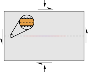Furthermore, provided $\sqrt {\alpha t}$ is sufficiently greater than $h$, we may reasonably neglect any fault-normal stress changes due to the swelling of the poroelastic layer about the source (Marck et al. Reference Marck, Savitski and Detournay2015). The medium containing the fault is assumed to be linearly elastic and its deformation, along with slip on the fault, may be in-plane or anti-plane. The in-plane case is illustrated in figure 1(a). The shear modulus of the medium is $\mu$ and the Poisson ratio $\nu$. We define the effective elastic modulus $\mu '=\mu /[2(1-\nu )]$ for the in-plane (mode-II) case and $\mu '=\mu /2$ for the anti-plane (mode-III) case. We denote the initial (pre-injection) fault shear stress $\tau$ (in-plane or anti-plane), the fault friction coefficient $f$, the initial total fault-normal compressive stress $\sigma$ and the initial effective normal stress $\sigma '=\sigma -p_o$, where $p_o$ is the pre-injection pore fluid pressure in the layer. The initial fault strength is $\tau _p=f\sigma '$.

Figure 1. Counter-clockwise: (a) Unbounded elastic body containing a fault, loaded remotely with fault-normal and shear stress $\sigma$, $\tau$. The fault is embedded within a thin poroelastic layer, assumed to be much more permeable than the surroundings. Fluid injected at $x=0$ diffuses along the fault as $\sqrt {\alpha t}$, inducing quasi-static slip out to a distance $a(t)$. The fault has constant friction coefficient $f$. (c) Black: relation between rupture growth factor $\lambda$ and a parameter reflecting the initial state of stress and injection pressure, where $\sigma '=\sigma -p_o$ and $p_o$ is pre-injection fault fluid pressure. Dashed: asymptotic behaviours, (3.5) and (3.8). (d) Same as bottom left, with abscissa arranged to occupy a finite interval. (b) Plot of self-similar slip distributions at three instants in time after the start of injection, $t=1$, 5 and 10 min, for the specific choices $\sigma =50\ \text {MPa}$, $\tau =12\ \text {MPa}$, $p_o=20\ \text {MPa}$, $\Delta p = 12\ \text {MPa}$, $f=0.5$, $\alpha _{hy}=0.01\ \text {m}^2\ \text {s}^{-1}$, $\mu =30\ \text {GPa}$, $\nu =1/4$, $\mu '=20\ \text {GPa}$. For these choices, the parameter $(1-\tau /\tau _p)\sigma '/\Delta p=0.5$. The corresponding self-similar slip distribution and factor $\lambda$ are given in table S1 in the supplementary material available at https://doi.org/10.1017/jfm.2021.825.

The fault obeys a Coulomb friction law: the local shear strength of the fault $\tau _s$ is a constant proportion of the local effective normal stress, with a constant coefficient of friction $f$,

(2.5)\begin{equation} \tau_s(x,t)=f[\sigma-p(x,t)].\end{equation}

Where sliding occurs, this strength must equal the shear stress on the fault. The shear stress can be decomposed into a sum of the initial shear stress $\tau$ plus quasi-static changes due to a distribution of slip $\delta$ (e.g. Rice Reference Rice1968), such that the stress–strength condition is

(2.6)\begin{equation} \tau_s(x,t)=\tau+\frac{\mu'}{\rm \pi}\int_{{-}a(t)}^{a(t)} \frac{\partial \delta(s,t)/\partial s}{s-x}\,\textrm{d}s, \end{equation}

where $x=\pm a(t)$ are the crack-tip locations.

3. Summary of results

After non-dimensionalizing, the problem is found to have the sole parameter

(3.1)\begin{equation} \left(1-\frac{\tau}{\tau_p}\right)\frac{\sigma'}{\Delta p}\end{equation}

that is bounded between 0 and 1. The upper bound denotes a marginally pressurized fault, where the fluid pressure increase is just sufficient to initiate sliding: $f[\sigma -(p_o+\Delta p)]=\tau$. The lower bound denotes a critically stressed fault, where the initial shear stress is equal to the initial shear strength: $\tau =\tau _p$.

The solution consists of a self-similar distribution of slip, in which the crack front grows as

(3.2)\begin{equation} a(t)=\lambda \sqrt{\alpha t} \end{equation}

and the slip distribution can be written as

(3.3)\begin{equation} \delta(x,t)\Rightarrow \delta(\bar{x}), \end{equation}

where the similarity coordinate is

(3.4)\begin{equation} \bar{x} = x/a(t). \end{equation}

The factor $\lambda$, to be solved for, determines whether the crack lags ($\lambda <1$) or outpaces ($\lambda >1$) the diffusion of pore pressure, which stretches as $\sqrt {\alpha t}$. Here $\lambda$ depends uniquely on the sole parameter (3.1), and that dependence is illustrated in figure 1(b) and tabulated at the top of table S1 in the supplementary material. The self-similar profile of slip, as it depends on $|x|/a(t)$, is also presented in the bottom of table S1 for several values of the parameter (3.1). Scaled plots of the self-similar profile for various values of $\lambda$ are shown in figure 2. In the limit that the parameter (3.1) approaches its end-member values, closed-form expressions for $\lambda$ and $\delta$ are available and provided below to leading order, with detailed derivations in the sections that follow.

Figure 2. (a) Self-similar distributions of slip $\delta$ with distance from injection point $x$, which is scaled by the crack half-length $a(t)=\lambda \sqrt {\alpha t}$. Solid red and black curves are numerical solutions to the full problem. Dashed curves are leading-order asymptotic solutions. Each curve corresponds to one value of $\lambda$ in the range $\lambda =10^{-3},10^{-2},\ldots ,10^3$. Black curves correspond to $\lambda =10^{-3},10^{-2},10^{-1},10^0$ from top to bottom, with the first three indistinguishable on this scale; red curves correspond to $\lambda =10^1,10^2,10^3$ from top to bottom. Cyan-dashed: solution for small $\lambda$, (3.6). Blue-dashed: ‘outer’ solutions for large $\lambda$, (3.9). To facilitate comparisons, two vertical scales are used: one for black and cyan-dashed curves, and another for red and blue-dashed curves. (b) For large values of $\lambda$, the distribution of slip is plotted over distances scaled by $\sqrt {\alpha t}$, which is much smaller than the crack length $a(t)$. This ‘inner’ behaviour is described by (3.10), a single numerical solution shown here as black-dashed curves. Curves correspond to $\lambda =10^1,10^2,10^3$ from bottom to top.

3.1. Marginally pressurized faults, $\tau \rightarrow f(\sigma '-\Delta p)$

In this limit the parameter $(1-\tau /\tau _p)\,\sigma '/\Delta p\rightarrow 1$, the factor $\lambda \ll 1$ (i.e. the rupture lags the diffusion of pore fluid pressure) and the relation between the two follows the asymptotic expansion

(3.5)\begin{equation} (1-\tau/\tau_p)\sigma'/\Delta p\approx 1-\frac{4}{{\rm \pi}^{3/2}}\lambda + O(\lambda^3) . \end{equation}

The slip distribution in this limit is

(3.6)\begin{equation} \delta(\bar{x})\approx\frac{\lambda^2 \sqrt{\alpha t}\, f \Delta p }{\mu'} \frac{2}{{\rm \pi}^{3/2}}\left(\sqrt{1-\bar{x}^2}-\bar{x}^2\,\text{atanh}\,\sqrt{1-\bar{x}^2}\right)+O(\lambda^4) \end{equation}

and the accumulation of slip at the centre is

(3.7)\begin{equation} \delta(0)\approx\frac{2}{{\rm \pi}^{3/2}} \frac{\lambda^2\sqrt{\alpha t}\ f\Delta p}{\mu'}+O(\lambda^4). \end{equation}

The derivation of this solution is detailed in § 5.

3.2. Critically stressed faults, $\tau \rightarrow \tau _p$

In this limit $(1-\tau /\tau _p)\,\sigma '/\Delta p\rightarrow 0$, $\lambda \gg 1$ (i.e. the rupture outpaces the diffusion of fluid pressure), and the asymptotic relation is

(3.8)\begin{equation} (1-\tau/\tau_p)\,\sigma'/\Delta p\approx \frac{2}{{\rm \pi}^{3/2}}\frac{1}{\lambda}+O(\lambda^{{-}3}) .\end{equation}

Similarly to the problem considered by GG12, the solution for slip can be decomposed into an outer solution on distances comparable to the rupture distance $a(t)$, and an inner solution on distances comparable to the diffusion length scale $\sqrt {\alpha t}$. The two solutions are matched at an intermediate distance.

The outer solution for the slip distribution is

(3.9)\begin{equation} \delta (\bar{x})\approx \frac{\sqrt{\alpha t}\, f \Delta p }{\mu'} \frac{2}{{\rm \pi}^{3/2}} \left(\text{atanh}\,\sqrt{1-\bar{x}^2}-\sqrt{1-\bar{x}^2}\right) +O(\lambda^{{-}2}), \end{equation}

where $\bar {x}$ is the similarity coordinate used above. The derivation of this solution may be found in § 6.

The inner solution is given by the expression

(3.10)\begin{equation} \delta(x/\sqrt{\alpha t}) \approx \delta(0) - \frac{\sqrt{\alpha t}\, f\Delta p}{\mu ' }\underline{\int_0^{x/\sqrt{\alpha t}}\left[\frac{1}{\rm \pi}\int_{-\infty}^\infty \frac{\text{erfc}(| \hat{s}|)}{\hat{x}-\hat{s}}\textrm{d}\hat{s}\right]\textrm{d}\hat{x}}+O(\lambda^{{-}2}). \end{equation}

The underlined portion is evaluated numerically and provided as a supplementary function $f(x/\sqrt {\alpha t})$ in table S2 with the similarity coordinate

(3.11)\begin{equation} \hat{x} = \frac{x}{\sqrt{\alpha t}}. \end{equation}

For large distances $x/\sqrt {\alpha t}$, $f$ behaves as

(3.12)\begin{equation} f(\hat{x})\approx\frac{2}{{\rm \pi}^{3/2}}\left(\ln \left | \hat{x} \right | +\frac{\gamma}{2}+1\right)+O\left(\hat{x}^{{-}2}\right) , \end{equation}

where $\gamma =0.57721566\ldots$ is the Euler–Maraschoni constant. Using this asymptotic behaviour to match the inner solution at large $x/\sqrt {\alpha t}$ with the outer solution at small $x/a(t)$ provides the slip at the centre

(3.13)\begin{equation} \delta(0)\approx \frac{\sqrt{\alpha t}\ f\Delta p}{\mu'}\frac{2}{{\rm \pi}^{3/2}}[\ln(2\lambda)+\gamma /2+O(\lambda^{{-}2})] \end{equation}

in the large $\lambda$ limit.

Other properties of $f(x/\sqrt {\alpha t})$ include

(3.14)\begin{equation} f''(\hat{x})={-}\frac{2}{{\rm \pi}^{3/2}}\exp(-\hat{x}^2) \textrm{Ei}(\hat{x}^2), \end{equation}

where ${Ei}(x)=-\int _{-x}^\infty \exp (-u)/u \,\textrm {d}u$ is the exponential integral, and in the limit that $x/\sqrt {\alpha t}$ is small, $f$ behaves as

(3.15)\begin{equation} f(\hat{x})\approx \frac{2}{{\rm \pi}^{3/2}}\,\hat{x}^2\left(\ln \frac{1}{|\hat{x}|} -\frac{\gamma}{2} +\frac{3}{2} \right)+O\left(\hat{x}^4 \ln |\hat{x}|\right) . \end{equation}

A detailed discussion of the inner solution and its matching to the outer solution, can be found in §§ 7 and 8.

3.3. Accumulation of slip at the injection point

Figures 3 and 4 show the solution for the peak slip, located at the injection point, as it depends on the parameter (3.1) or the factor $\lambda$. An approximation of peak slip at the injection point that respects the asymptotic behaviour at both critically stressed and marginally pressurized limits – (3.7) and (3.13) – and is to within 5 % error over the intervening range of $\lambda$, is

(3.16)\begin{equation} \delta(0)\approx \frac{\lambda\sqrt{\alpha t}\, f \Delta p }{\mu'} \frac{2}{{\rm \pi}^{3/2}}\frac{\lambda}{1+\lambda^2/[\ln(6+2\lambda) +\gamma/2]}. \end{equation}

Figure 3. The maximum slip, which occurs at $x=0$, as it relates to the factor $\lambda$ shown as (a) semi-log and (b) log–log plots. Red-dashed: end-member scalings at small $\lambda$, (3.7), and at large $\lambda$, (3.13). Blue-dashed: approximation of $\delta (0)$ for all $\lambda$, (3.16).

Figure 4. The peak slip as it relates to the problem parameter $(1-\tau /\tau _p)\,\sigma '/\Delta p$. Red-dashed: scalings as the parameter approaches its bounds, derived from (3.7) and (3.13) and the asymptotic relations between the parameter and $\lambda$, (3.5) and (3.8).

Figure 5. Self-similar distribution of slip $\delta$, less the first-order term, (5.6), in the asymptotic expansion for slip (5.4) in the marginally pressurized limit (small $\lambda$). From top to bottom, black curves correspond to the difference for $\lambda =2,1,{1}/{2},{1}/{4},{1}/{8}$. The cyan-dashed curve is the second-order term of the expansion, (5.7).

4. Non-dimensionalization and solution to full problem

Combining (2.3)–(2.6) and rearranging leads to the non-dimensionalized equation

(4.1)\begin{equation} \left(1-\frac{\tau}{\tau_p}\right)\frac{\sigma'}{\Delta p}-\text{erfc}\left| \lambda\bar{x}\right|={-}\frac{1}{\rm \pi}\int_{{-}1}^{1}\frac{\textrm{d}\bar{\delta}/\textrm{d}\bar{s}}{\bar{x}-\bar{s}}\, \textrm{d}\bar{s},\end{equation}

where we have used $x=a(t)\bar {x}$, $a(t)=\lambda \sqrt {\alpha t}$ and $\delta (x,t)=\bar {\delta }[x/a(t)]a(t)f\Delta p/\mu '$. The solution we seek is the slip distribution $\bar {\delta }$ and the crack-growth prefactor $\lambda$, including their dependence on the problem parameter $(1-\tau /\tau _p)/\sigma '/\Delta p$.

We begin by looking for the solution for $\lambda$. To do so, we first note that to avoid a singularity in shear stress ahead of the crack tips, which is necessary because the Coulomb friction requirement implies a finite shear strength of the interface, the crack-tip stress intensity factors of the rupture must be zero. This condition implies (Appendix A)

(4.2)\begin{equation} \left(1-\frac{\tau}{\tau_p}\right)\frac{\sigma'}{\Delta p}=\frac{1}{\rm \pi}\int_{{-}1}^1\frac{\text{erfc}|\lambda x|}{\sqrt{1-x^2}}\,{\textrm{d}\kern0.7pt x} \end{equation}

which provides an implicit solution for $\lambda$ as it depends on the problem parameter. This relation is easily determined numerically since, for a given $\lambda$, the integrand on the right-hand side can be evaluated by Gauss–Chebyshev quadrature (Appendix B). The behaviour at large and small values of $\lambda$, (3.5) and (3.8), is found by asymptotic approximation of the integral.

To solve for $\bar {\delta }$, we note that (4.1) may be inverted for $\textrm {d}\bar {\delta }/\textrm {d}\kern0.7pt \bar {x}$ (Appendix A),

(4.3)\begin{equation} \frac{\textrm{d}\bar \delta}{\textrm{d}\bar{x}}={-}\frac{\sqrt{1-\bar{x}^2}}{\rm \pi}\int_{{-}1}^1\frac{\text{erfc}|\lambda \bar{s}|}{\sqrt{1-\bar{s} ^2}}\frac{1}{\bar{x}-\bar{s}}\,\textrm{d}\bar{s} . \end{equation}

After having determined $\lambda$ via (4.2), the right-hand side may be numerically evaluated and integrated to arrive to $\bar {\delta }(\bar {x})$ using a Gauss–Chebyshev quadrature for singular integrals (Erdogan, Gupta & Cook Reference Erdogan, Gupta and Cook1973; Viesca & Garagash Reference Viesca and Garagash2018). The numerical solution of (4.2) and (4.3) for $\lambda$ and $\bar {\delta }(\bar {x})$ is detailed in Appendix B.

5. Solution in the marginally pressurized limit

For $\lambda \ll 1$, we may use the expansion of the function

(5.1)\begin{equation} \text{erfc}|\lambda \bar{x}|\approx 1-\frac{2}{\sqrt{\rm \pi}}|\lambda \bar{x}|+\frac{2}{3\sqrt{\rm \pi}}|\lambda \bar{x}|^3+\ldots\end{equation}

to expand the integral in (4.2) as

(5.2)\begin{equation} \left(1-\frac{\tau}{\tau_p}\right)\frac{\sigma'}{\Delta p}=\int_{{-}1}^{1}\frac{\text{erfc}|\lambda x|}{\sqrt{1-x^2}}{\textrm{d}\kern0.7pt x}\approx1-\frac{4}{{\rm \pi}^{3/2}}\lambda +\frac{8}{9{\rm \pi}^{3/2}}\lambda^3+O(\lambda^5). \end{equation}

In turn, we use (5.1) and (5.2) to reduce (4.1) to

(5.3)\begin{equation} \frac{1}{\rm \pi}\int_{{-}1}^{1}\frac{\textrm{d}\bar{\delta}/\textrm{d}\bar{s}}{\bar{x}-\bar{s}}\textrm{d}\bar{s} \approx \lambda\left(\frac{4}{{\rm \pi}^{3/2}}-\frac{2}{\sqrt{\rm \pi}}|\bar{x}|\right) + \lambda^3\left(-\frac{8}{9{\rm \pi}^{3/2}}+\frac{2}{3\sqrt{\rm \pi}}|x|^3\right)+O(\lambda^5). \end{equation}

We write the solution to the above equation as the perturbation expansion

(5.4)\begin{equation} \bar{\delta}(\bar{x})\approx \lambda\delta_0(\bar{x})+\lambda^3\delta_1 (\bar{x})+O(\lambda^5), \end{equation}

where $\delta _0$ and $\delta _1$ satisfy

(5.5a,b)\begin{align} \frac{1}{\rm \pi}\int_{{-}1}^{1}\frac{\textrm{d}\delta_0/\textrm{d}\bar{s}}{\bar{x} -\bar{s}}\textrm{d}\bar{s}= \frac{4}{{\rm \pi}^{3/2}}-\frac{2}{\sqrt{\rm \pi}}|\bar{x}|{,} \quad \frac{1}{\rm \pi}\int_{{-}1}^{1}\frac{\textrm{d}\delta_1/\textrm{d}\bar{s}}{\bar{x}-\bar{s}}\textrm{d}\bar{s}={-}\frac{8}{9{\rm \pi}^{3/2}}-\frac{2}{3\sqrt{\rm \pi}}|\bar{x}|^3. \end{align}

The solutions to which

(5.6)$$\begin{gather} \delta_0(\bar{x})=\frac{2}{{\rm \pi}^{3/2}} \left(\sqrt{1-\bar{x}^2}-\bar{x}^2 \,\text{atanh}\, \sqrt{1-\bar{x}^2}\right), \end{gather}$$

(5.7)$$\begin{gather}\delta_1(\bar{x})= \frac{1}{3{\rm \pi}^{3/2}}\left((\bar{x}^2-2)\sqrt{1-\bar{x}^2}+\bar{x}^4 \,\text{atanh}\,\sqrt{1-\bar{x}^2}\right) \end{gather}$$

are found by the linear superposition of particular solutions to the general problem

(5.8)\begin{equation} g(x)=\frac{1}{\rm \pi}\int_{{-}1}^1 \frac{h'(s)}{x-s}\textrm{d}s \end{equation}

that are provided in table 1 and found following Appendix A. Using (5.4), the slip at the injection point in the marginally pressurized limit evaluates to

(5.9)\begin{equation} \delta(0)\approx\frac{\lambda\sqrt{\alpha t}\ f\Delta p}{\mu'}\left(\frac{2}{{\rm \pi}^{3/2}}\lambda-\frac{2}{3{\rm \pi}^{3/2}}\lambda^3+O(\lambda^5) \right) . \end{equation}

Table 1. Select solutions $h(x)$ to the problem $g(x)=({1}/{{\rm \pi} })\int _{-1}^1({h'(s)}/({x-s}))\,\textrm {d}s$, with $h(\pm 1)=0$.

6. Outer solution in the critically stressed limit

We now look for an asymptotic expansion of the solution in the critically stressed limit, in which the rupture front outpaces fluid pressure diffusion, $\lambda \gg 1$. As noted by GG12 for their problem, the solution consists of an outer solution on distances comparable to the rupture distance $a(t)$ and an inner solution on distances comparable to $\sqrt {\alpha t}$. To look for the outer solution, we solve for the slip distribution satisfying (4.1) after expanding the two terms on the left-hand side in the large $\lambda$ limit. We begin by considering the expansion of the following function as $\lambda \rightarrow \infty$:

(6.1)\begin{equation} \frac{\text{erfc}|u|}{\sqrt{1-(u/\lambda)^2}}\approx \text{erfc}|u|+\frac{1}{2\lambda^2}u^2\,\text{erfc}|u|+O(\lambda^{{-}4}).\end{equation}

This function appears in the integral (4.2) following the change of variable $u=\lambda \bar {x}$, such that

(6.2)\begin{equation} \left(1-\frac{\tau}{\tau_p}\right)\frac{\sigma'}{\Delta p}=\frac{1}{{\rm \pi}\lambda}\int_{-\lambda}^{\lambda}\frac{\text{erfc}|u|}{\sqrt{1-(u/\lambda)^2}}\,\textrm{d}u \approx\frac{2}{{\rm \pi}^{3/2}}\frac{1}{\lambda} +\frac{1}{3{\rm \pi}^{3/2}}\frac{1}{\lambda^3}+O(\lambda^{{-}5}) . \end{equation}

In addition, we perform a multipole expansion of the distribution (Appendix C)

(6.3)\begin{equation} \text{erfc}|\lambda \bar{x}| \approx p_0\delta_D (\bar{x})-p_1\delta_D'(\bar{x})+p_2 \delta''_D(\bar{x})+O(\lambda^{{-}5}), \end{equation}

where $\delta _D$ is the Dirac delta and its first and second derivatives, $\delta _D'(x)$ and $\delta _D''(x)$, with the properties

(6.4a–c)\begin{equation} \int_{-\infty}^\infty \delta_D(x)\,\textrm{d}\kern0.7pt x=1,\quad \int_{-\infty}^\infty x\delta'_D(x)\,\textrm{d}\kern0.7pt x=1,\quad \int_{-\infty}^\infty \frac{x^2}{2} \delta''_D(x)\,\textrm{d}\kern0.7pt x=1, \end{equation}

and where the coefficients

(6.5)$$\begin{gather} p_0=\int_{{-}1}^1 \text{erfc}|\lambda\bar{x}|\,\textrm{d}\bar{x}=\frac{1}{\lambda} \int_{-\lambda}^\lambda \text{erfc}|\hat{x}|\,\textrm{d}\hat{x}=\frac{2}{\sqrt{\rm \pi}}\frac{1}{\lambda}+ O(\exp(-\lambda^2)/\lambda), \end{gather}$$

(6.6)$$\begin{gather}p_1=\int_{{-}1}^1 \bar{x} \,\text{erfc}|\lambda\bar{x}|\,\textrm{d}\bar{x}=0, \end{gather}$$

(6.7)$$\begin{gather}p_2=\int_{{-}1}^1 \frac{\bar{x}^2}{2} \text{erfc}|\lambda\bar{x}|\,\textrm{d}\bar{x}= \frac{1}{3\sqrt{\rm \pi}}\frac{1}{\lambda^3}+O(\exp(-\lambda^2)/\lambda^{3}) \end{gather}$$

exhibit beyond-all-orders decay at large $\lambda$ at the rate $\exp (-\lambda ^2)$, following the leading-order term. With (6.2) and (6.3), the equation governing the slip distribution (4.1) becomes

(6.8)\begin{align} \frac{1}{\rm \pi}\int_{{-}1}^{1}\frac{\textrm{d}\bar{\delta}/\textrm{d}\bar{s}}{\bar{x}-\bar{s}}\,\textrm{d}\bar{s} \approx \frac{1}{\lambda}\left(-\frac{2}{{\rm \pi}^{3/2}} + \frac{2}{\sqrt{\rm \pi}}\,\delta_D(\bar{x}) \right) +\frac{1}{\lambda^3} \left(-\frac{1}{3{\rm \pi}^{3/2}} + \frac{1}{3\sqrt{\rm \pi}}\,\delta''_D(\bar{x}) \right) +O(\lambda^{{-}5}). \end{align}

As for the marginally pressurized case, we look for a solution in the form of a perturbation expansion

(6.9)\begin{equation} \bar{\delta}(\bar{x})\approx \frac{1}{\lambda}\delta_0(\bar{x})+\frac{1}{\lambda^3} \delta_1(\bar{x})+O(\lambda^{{-}5}), \end{equation}

where $\delta _0$ and $\delta _1$ now satisfy

(6.10a,b) \begin{equation} \frac{1}{\rm \pi}\int_{{-}1}^{1}\frac{\textrm{d}\delta_0/\textrm{d}\bar{s}}{\bar{x}-\bar{s}}\,\textrm{d}\bar{s}={-}\frac{2}{{\rm \pi}^{3/2}}+\frac{2}{\sqrt{\rm \pi}}\,\delta_D(\bar{x}), \quad \frac{1}{\rm \pi}\int_{{-}1}^{1}\frac{\textrm{d}\delta_1/\textrm{d}\bar{s}}{\bar{x}-\bar{s}}\,\textrm{d}\bar{s}={-}\frac{1}{3{\rm \pi}^{3/2}}+\frac{1}{3\sqrt{\rm \pi}}\,\delta''_D(\bar{x}) \end{equation}

and the solutions

(6.11)$$\begin{gather} \delta_0(\bar{x})=\frac{2}{{\rm \pi}^{3/2}}\left(\text{atanh}\, \sqrt{1-\bar{x}^2}-\sqrt{1-\bar{x}^2}\right), \end{gather}$$

(6.12)$$\begin{gather}\delta_1(\bar{x})=\frac{1}{3{\rm \pi}^{3/2}}\left(\frac{\sqrt{1-\bar{x}^2}} {\bar{x}^2}-\sqrt{1-\bar{x}^2}\right) \end{gather}$$

are again found by superposing solutions provided in table 1.

From the above, the outer solution for slip near $\bar {x} =0$ has the behaviour

(6.13)\begin{align} \delta(\bar{x})&\approx \frac{\lambda\sqrt{\alpha t}\ f\Delta p}{\mu'}\left[\frac{1}{\lambda}\frac{2}{{\rm \pi}^{3/2}} \left(\log\frac{2}{|\bar{x}|}-1 + \frac{\bar{x}^2}{4}+O(\bar{x}^4)\right)\right.\nonumber\\ &\quad\left.+\frac{1}{\lambda^3}\frac{1}{3{\rm \pi}^{3/2}} \left(\frac{1}{\bar{x}^2}-\frac{3}{2}+O(\bar{x}^2) \right)+O(\lambda^{{-}5})\right] . \end{align}

7. Inner solution in the critically stressed limit

To examine the behaviour of slip on the diffusive length scale $\sqrt {\alpha t}$, we perform a change of variable to the scale distance $\hat {x} = \lambda \bar {x} = x/\sqrt {\alpha t}$, such that (4.3) becomes

(7.1)\begin{equation} \lambda\frac{\textrm{d}\bar \delta}{\textrm{d}\hat{x}}={-}\frac{\sqrt{1-(\hat{x}/\lambda)^2}}{\rm \pi}\int_{-\lambda}^\lambda\frac{\text{erfc}|\hat{s}|}{\sqrt{1-(\hat{s}/\lambda)^2}}\frac{1}{\hat{x}-\hat{s}}\,\textrm{d}\hat{s}.\end{equation}

Rescaling slip as $\hat {\delta } = \lambda \bar {\delta } = \delta /(\sqrt {\alpha t}\ f\Delta p/\mu ')$, we perform a series expansion of the square-root terms for large $\lambda$,

(7.2)\begin{equation} \frac{\textrm{d}\hat{\delta}}{\textrm{d}\hat{x}}\approx{-}\frac{1}{\rm \pi}\left(1-\frac{1}{\lambda^2}\frac{\hat{x}^2}{2}+ O(\lambda^{{-}4})\right)\int_{-\lambda}^\lambda\left(\text{erfc}|\hat{s}|+ \frac{1}{\lambda^2}\frac{\hat{s}^2}{2}\text{erfc}|\hat{s}|+O(\lambda^{{-}4})\right)\frac{1}{\hat{x}-\hat{s}}\,\textrm{d}\hat{s}, \end{equation}

and regroup terms of similar order,

(7.3) \begin{align} \frac{\textrm{d}\hat \delta}{\textrm{d}\hat{x}}\approx{-}\frac{1}{\rm \pi}\int_{-\lambda}^\lambda\frac{\text{erfc}|\hat{s}|}{\hat{x} - \hat{s}}\,\textrm{d}\hat{s}+\frac{1}{\lambda^2}\left(\frac{\hat{x}^2}{2}\frac{1}{\rm \pi}\int_{-\lambda}^\lambda \frac{\text{erfc}|\hat{s}|}{\hat{x}-\hat{s}}\,\textrm{d}\hat{s}-\frac{1}{\rm \pi}\int_{-\lambda}^\lambda \frac{(\hat{s}^2/2)\text{erfc}|\hat{s}|}{\hat{x} - \hat{s}}\,\textrm{d}\hat{s}\right)+O(\lambda^{{-}4}). \end{align}

Given the beyond-all-orders decay, for modestly large values of $\hat {s}$, of the term $\text {erfc}|\hat {s}|\approx \exp (-\hat {s}^2)/(\sqrt {{\rm \pi} }\hat {s})$ appearing in all of the integrands above, the limits of the integrals may pass to $\infty$ without consequence for the above expansion in powers of $\lambda$. Hence,

(7.4) \begin{align} \frac{\textrm{d}\hat{\delta}}{\textrm{d}\hat{x}}&\approx{-}\frac{1}{\rm \pi}\int_{-\infty}^\infty \frac{\text{erfc}|\hat{s}|}{\hat{x} -\hat{s}}\,\textrm{d}\hat{s}+\frac{1}{\lambda^2}\left(\frac{\hat{x}^2}{2}\frac{1}{\rm \pi}\int_{-\infty}^\infty \frac{\text{erfc}|\hat{s}|}{\hat{x}-\hat{s}}\,\textrm{d}\hat{s}-\frac{1}{\rm \pi}\int_{-\infty}^\infty \frac{(\hat{s}^2/2)\text{erfc}|\hat{s}|}{\hat{x} - \hat{s}}\,\textrm{d}\hat{s}\right)\nonumber\\ &\quad +O(\lambda^{{-}4}) . \end{align}

The above integrals are Hilbert transforms, defined as

(7.5)\begin{equation} \mathcal{H}[f(s)]=\frac{1}{\rm \pi}\int_{-\infty}^\infty \frac{f(s)}{x-s}\,\textrm{d}s \end{equation}

which have the property

(7.6)\begin{align} \mathcal{H}[s^2f(s)]&=\mathcal{H}[(s^2-x^2+x^2)f(s)]\nonumber\\ &=x^2\mathcal{H}[f(s)]+\mathcal{H}[(s-x)(s+x)f(s)]\nonumber\\ &=x^2\mathcal{H}[f(s)]-\frac{1}{\rm \pi}\int_{-\infty}^{\infty}sf(s)\,\textrm{d}s-\frac{x}{\rm \pi}\int_{-\infty}^{\infty}f(s)\, \textrm{d}s \end{align}

that, when applied to the third integral in (7.4),

(7.7) \begin{equation} \frac{1}{\rm \pi}\int_{-\infty}^\infty \frac{(\hat{s}^2/2)\text{erfc}|\hat{s}|}{\hat{x} - \hat{s}}\,\textrm{d}\hat{s}=\frac{\hat{x}^2}{2}\frac{1}{\rm \pi}\int_{-\infty}^\infty \frac{\text{erfc}|\hat{s}|}{\hat{x}-\hat{s}}\,\textrm{d}\hat{s} -\frac{\hat{x}}{{\rm \pi}^{3/2}}, \end{equation}

leads to the reduction of (7.4) to

(7.8)\begin{equation} \frac{\textrm{d}\hat{\delta}}{\textrm{d}\hat{x}}\approx{-}\frac{1}{\rm \pi}\int_{-\infty}^\infty\frac{\text{erfc}|\hat{s}|}{\hat{x} - \hat{s}}\,\textrm{d}\hat{s}+\frac{1}{\lambda^2}\frac{\hat{x}}{{\rm \pi}^{3/2}} +O(\lambda^{{-}4}). \end{equation}

Subsequently integrating from 0 to $\hat {x}$, we find the inner solution to within a yet-undetermined constant $\delta (0)$,

(7.9) \begin{equation} \hat{\delta}(\hat{x}) \approx \hat{\delta} (0) - \underline{\int_0^{\hat{x}}\left[\frac{1}{{\rm \pi} }\int_{-\infty}^\infty \frac{\text{erfc}|s|}{x -s}\,\textrm{d} s\right]{\textrm{d}\kern0.7pt x}} + \frac{1}{\lambda^2}\frac{\hat{x}^2}{2{\rm \pi}^{3/2}}+O(\lambda^{{-}4}) . \end{equation}

We define the underlined term as the function $f(\hat {x})$ whose first derivative is the Hilbert transform

(7.10)\begin{equation} f'(\hat{x}) = \frac{1}{\rm \pi}\int_{-\infty}^\infty\frac{\text{erfc}|s| }{\hat{x} -s}\,\textrm{d}s. \end{equation}

Since the transform commutes with derivatives, $[\mathcal {H}(g)]'=\mathcal {H}(g')$, we find that $f''$ has the concise expression

(7.11)\begin{equation} f''(\hat{x})={-}\frac{2}{{\rm \pi}^{3/2}}\int_{-\infty}^\infty \frac{\text{sign}(s)\exp({-}s^2) }{\hat{x} -s}\,\textrm{d}s \end{equation}

which may be further simplified to

(7.12)\begin{align} f''(\hat{x})&={-}\frac{2}{{\rm \pi}^{3/2}}\exp(-\hat{x}^2)\int_0^\infty \frac{\exp(\hat{x}^2-s^2)}{\hat{x}^2-s^2}2s\,\textrm{d}s\nonumber\\ &={-}\frac{2}{{\rm \pi}^{3/2}}\exp(-\hat{x}^2)\int_{-\hat{x}^2}^\infty\frac{\exp({-}u)}{u}\,\textrm{d}u\nonumber\\ &={-}\frac{2}{{\rm \pi}^{3/2}}\exp(- \hat{x}^2)\textrm{Ei}(\tilde{x}^2), \end{align}

with the change of variable $u=s^2-\hat {x}^2$ used in the intermediate step. In figure 6 we plot $f(\hat {x})$ found by numerically integrating twice the expression for $f''(\hat {x})$, (7.12).

Figure 6. Spatio-temporal component, $f(x/\sqrt {\alpha t})$, of ‘inner’ solution for slip $\delta$ in the critically stressed limit, (3.10). Shown in black on linear (a), log–linear (b) and logarithmic (c) axes. Red- and blue-dashed curves: outer and inner asymptotic behaviour of $f$, (3.12) and (3.15).

For $\hat {x}$ near 0,

(7.13)\begin{equation} f''(\hat{x})={-}\frac{2}{{\rm \pi}^{3/2}}\left(\ln|\hat{x}|+\gamma\right)+O(\hat{x}^2) \end{equation}

and upon integrating twice with $f(0)=f'(0)=0$, the behaviour of $f$ in this region is

(7.14)\begin{equation} f(\hat{x})=\frac{2}{{\rm \pi}^{3/2}}\hat{x}^2\left(\ln\frac{1}{|\hat{x}|}-\frac{\gamma}{2}+\frac{3}{2}\right)+O(\hat{x}^4\ln|\hat{x}|). \end{equation}

For large $\hat {x}$,

(7.15)\begin{equation} f''(\hat{x})={-}\frac{2}{{\rm \pi}^{3/2}}\left(\frac{1}{\hat{x}^2}+\frac{1}{\hat{x}^4}\right)+O(\hat{x}^{{-}6}). \end{equation}

Upon integrating twice with the condition that $f'(\infty )=0$,

(7.16)\begin{equation} f(\hat{x})= c + \frac{2}{{\rm \pi}^{3/2}}\left(\ln{|\hat{x}|}-\frac{1}{6\hat{x}^2}\right) +O(\hat{x}^{{-}4}) , \end{equation}

where $c$ is a yet-undetermined constant of integration.

We determine the constant $c$ following an approach used by GG12, in which the order of integration in (7.9) is swapped leading to an alternative expression for $f(\hat {x})$,

(7.17)\begin{equation} f(\hat{x})=\int_0^{\hat{x}}\left[\frac{1}{{\rm \pi} }\int_{-\infty}^\infty \frac{\text{erfc}|s|}{x -s}\textrm{d} s\right]{\textrm{d}\kern0.7pt x}=\frac{1}{{\rm \pi} }\int_{-\infty}^\infty \text{erfc}|s| \,\ln\left |1-\frac{\hat{x}} {s}\right | \textrm{d}s, \end{equation}

and the expansion $\ln |1-\hat {x}/s |=\ln |\hat {x}| - \ln |s|+\ln |s/\hat {x}-1|$ is used to decompose the latter integral for $f(\hat {x})$ into the sum

(7.18)\begin{align} f(\hat{x}) &= \frac{1}{{\rm \pi} }\int_{-\infty}^\infty \text{erfc}|s|\,\textrm{d}s \ln|\hat{x}| -\frac{1}{{\rm \pi} }\int_{-\infty}^\infty \text{erfc}|s|\ln|s|\,\textrm{d}s+ \frac{1}{{\rm \pi} }\int_{-\infty}^\infty \text{erfc}|s|\ln\left | \frac{s}{\hat{x}}-1\right |\textrm{d}s \end{align}

(7.19)\begin{align} &=\frac{2}{{\rm \pi}^{3/2}}\ln|\hat{x}| +\frac{2}{{\rm \pi}^{3/2}}\left(1+\frac{\gamma}{2}\right)+\frac{1}{{\rm \pi} } \int_{-\infty}^\infty \text{erfc}|s|\ln\left | \frac{s}{\hat{x}}-1\right |\textrm{d}s. \end{align}

Comparing (7.16) and (7.19), we see that the asymptotic behaviour of the last integral in (7.19), for large $\hat {x}$, is given by the terms in (7.16), excluding the constant and the logarithmic terms. We also retrieve the value of the constant $c$,

(7.20)\begin{equation} c=\frac{2}{{\rm \pi}^{3/2}}\left(1+\frac{\gamma}{2}\right) \end{equation}

from which we conclude that the inner solution for slip has the asymptotic behaviour at large $\hat {x}$,

(7.21)\begin{align} \delta(\hat{x}) &\approx \delta(0)-\frac{\sqrt{\alpha t}\ f\Delta p}{\mu'}\left[\frac{2}{{\rm \pi}^{3/2}}\left(1+\frac{\gamma}{2}+\ln{|\hat{x}|}- \frac{1}{6|\hat{x}|^2}+O(\hat{x}^{{-}4})\right)\right.\nonumber\\ &\left.\quad - \frac{1}{\lambda^2}\frac{\hat{x}^2}{2{\rm \pi}^{3/2}} + O(\lambda^{{-}4})\right]. \end{align}

8. Matching inner and outer solutions

We match the outer and inner solutions by equating (6.13) and (7.21) and solving for $\delta (0)$, the slip at the centre in the critically stressed limit

(8.1)\begin{equation} \delta(0)\approx\frac{\sqrt{\alpha t}\ f\Delta p}{\mu'}\frac{2}{{\rm \pi}^{3/2}}\left[\frac{\gamma}{2}+\ln(2\lambda)-\frac{1}{4\lambda^2}+O(\lambda^{{-}4})\right] \end{equation}

which completes the expression for the inner solution (7.9). In figure 7 we overlay the inner and outer solutions, to first and second order, above the full solutions for several large values of $\lambda$. The intermediate matching of the solutions is evident in the overlap of the dashed curves. As an aside, we can now show approximations to the slip at the centre to first and second order in both the critically stressed and marginally pressurized limits in figure 8. For comparison, we also show the full solution, as well as the ad hoc approximation (3.16) constructed using the first-order asymptotics.

Figure 7. Self-similar distribution of slip in the critically stressed limit (large $\lambda$). In this limit the rupture extent $a(t)$ outpaces the diffusive distance $\sqrt {\alpha t}$. (a,b) Black curves from right to left correspond to full solutions for the self-similar slip profiles for $\lambda =10,100,1000$. (a) Red-dashed and blue-dashed lines correspond to outer and inner solution expansion to first order. (b) Red-dashed and blue-dashed lines correspond to outer and inner solution expansion to second order. Outer solution is given by (6.9)–(6.12). Inner solution given by (7.9).

Figure 8. Comparison of approximations to the full solution of peak fault slip (black curve) in the vicinity of $\lambda =1$. First- and second-order approximations in the marginally pressurized and critically stressed limits, given respectively by (5.9) and (8.1), are shown as red-dashed and red-dot–dashed curves. Blue-dashed curve: approximation provided for all values of $\lambda$, (3.16).

Using the inner and outer solutions, we construct a composite approximation (e.g. Hinch Reference Hinch1991)

(8.2)\begin{equation} \delta_{comp}(\bar{x})=\delta_{in}(\lambda \bar{x})+\delta_{out}(\bar{x})-\delta_{overlap}(\bar{x}), \end{equation}

where $\delta _{in}$ and $\delta _{out}$ are the inner and outer solutions, (7.9) and (6.9), and

(8.3)\begin{equation} \delta_{overlap}(\bar{x})=\frac{2}{{\rm \pi}^{3/2}}\left(\log\frac{2}{\bar{x}}-1+\frac{\bar{x}^2}{4}\right)+\frac{1}{\lambda^2} \frac{1}{3{\rm \pi}^{3/2}}\left(\frac{1}{\bar{x}^2}-\frac{3}{2}\right)+O(\lambda^{{-}4}) \end{equation}

is their common intermediate form. In figure 9 we compare the full numerical solution against the inner, outer and composite solutions for a modestly large value of $\lambda =5$. The composite solution has an approximate error of O($\lambda ^{-(n+2)}$), where $n=2\text { or 4}$ is the order neglected in the asymptotic expansion.

Figure 9. Solution for self-similar slip profile in black for $\lambda =5$. (a,b) Superimposed blue- and red-dashed curves, respectively, showing inner and outer solutions to (a) leading and (b) next order. (c) Superposition of leading and next-order composite solutions as blue- and red-dashed curves. (d) The difference between the self-similar solution and the composite solutions at leading and next order are respectively the blue and red-dashed curves. (e,f) Semi-logarithmic plots comparing the leading- and next-order composite solutions, in blue- and red-dashed curves, to the self-similar solution, in black.

9. Summary and conclusion

The quasi-static rupture of a fault driven by a source of fluids has been studied in detail. Tracking the rupture of the fault corresponds to a free boundary problem for which both the size of the slipping domain and the distribution of slip within must be solved. Both depend on a single dimensionless parameter whose limits correspond either to a fault whose initial, pre-injection shear stress is relatively close to the fault's pre-injection shear strength or to a fluid pressure increase that is marginally sufficient to induce sliding. Because the problem involves contact between elastic half-spaces, interactions between points on the fault are non-local, in that slip in one location induces changes in the shear stress over the entire fault plane. The resulting equation governing slip evolution is an integro-differential equation. In addition to the crack-tip boundary condition that slip vanishes at the rupture front, the condition determining the free boundary is the absence of a stress singularity ahead of the rupture front, which corresponds to the boundary condition that the gradient of slip also vanishes at the rupture front. Moreover, because the friction coefficient is held constant, there is an absence of an elasto-frictional length scale that may be otherwise present in problems for which friction depends explicitly on slip or its history. Correspondingly, the only length scale in the problem is the diffusive length $\sqrt {\alpha t}$ with the consequence that spatial dependence of slip scales directly with this length scale, implying the self-similar propagation of slip.

In a fashion similar to the earthquake-nucleation problem considered by GG12, we present asymptotic perturbation expansion solutions in the marginally pressurized and critically stressed limits and tabulate numerical solutions for the intervening cases. In the critically stressed limit, the problem has both an inner solution on the scale of diffusion and an outer solution on the scale of the crack front. An advantage of the posed problem is that the marginally pressurized expansion and the outer solution of the critically stressed limit are expressible in concise closed form. For the latter, we develop a multipole expansion method to develop successive approximations of a distributed loading beyond a point-force approximation. The leading-order term of the inner solution of the critically stressed limit is solved numerically and tabulated. Key findings include that the rupture run-out distance from the point of injection follows $a(t)=\lambda \sqrt {\alpha t}$, where $\lambda$ is an amplification factor, originally solved for and presented by Bhattacharya & Viesca (Reference Bhattacharya and Viesca2019). As noted there, if we denote the dimensionless problem parameter as $T\equiv (1-\tau /\tau _p)\sigma '/\Delta p$, then in the marginally pressurized limit $\lambda \approx ({\rm \pi} ^{3/2}/4)(1-T)$ and in the critically stressed limit $\lambda \approx (2/{\rm \pi} ^{3/2}) T^{-1}$. Furthermore, in the marginally pressurized limit, slip accumulates as $\delta \sim \lambda ^2\sqrt {\alpha t}\ f\Delta p/\mu '$. In the critically stressed limit, slip accumulates as $\delta \sim \sqrt {\alpha t}\ f\Delta p/\mu '$ on inner distances of the order $\sqrt {\alpha t}$ from the injection point and as $\delta \sim \lambda ^{-2}\sqrt {\alpha t}\ f\Delta p/\mu '$ at distances comparable to the rupture length $\lambda \sqrt {\alpha t}$.