


1. Introduction
The so-called ‘traditional approximation’ (Eckart Reference Eckart1960; Gerkema et al. Reference Gerkema, Zimmerman, Maas and van Haren2008; Lucas, McWilliams & Rousseau Reference Lucas, McWilliams and Rousseau2017) describes the neglect of the meridional (north–south) component of the planetary rotation vector. This approximation is justified by a scaling argument and valid for flows in which the vertical length scales are small compared with the horizontal length scales and the vertical velocities are small. While the traditional approximation is generally accurate for oceanic and atmospheric flows, the effects of the neglected rotation component – referred to here as non-traditional effects – can still be important in some problems, particularly if the vertical velocities are large or the traditional rotation vector vanishes.
For flows with strong vertical velocities, non-traditional rotation can have a variety of effects such as introducing directional dependence in Ekman flows (Coleman, Ferziger & Spalart Reference Coleman, Ferziger and Spalart1990; McWilliams & Huckle Reference McWilliams and Huckle2006) and tilting convective plumes in deep convection (Garwood Reference Garwood1991; Sheremet Reference Sheremet2004). Near the equator, the traditional Coriolis parameter is small and non-traditional rotation dominates. This results in a different form of geostrophic balance (de Verdière & Schopp Reference de Verdière and Schopp1994) in which horizontal density gradients are balanced by the meriodionally sheared velocity and can lead to the emergence of new phenomena such as the deep equatorial jets studied by Hua, Moore & Gentil (Reference Hua, Moore and Gentil1997).
Non-traditional effects also play an important role in the dynamics of internal waves (Gerkema & Shira Reference Gerkema and Shira2005; Gerkema et al. Reference Gerkema, Zimmerman, Maas and van Haren2008), particularly in the case of near-inertial waves where they act as a singular perturbation, resulting in a qualitatively different behaviour to the traditional system even when a scaling argument would suggest these effects are small. This perturbation corresponds to the existence of a range of trapped sub-inertial modes which vanish under the traditional approximation. Other effects include increasing the critical latitude at which internal waves can no longer propagate and modifying the reflection off a sloping bottom (Gerkema Reference Gerkema2006).
Ocean fronts are regions of strong horizontal buoyancy gradient and are common features in the upper ocean. These fronts typically occur on horizontal scales of around  $1 - 10\ \textrm {km}$ and exist in a state close to turbulent thermal wind (TTW) balance – the three way balance between the Coriolis force, horizontal pressure gradients and the vertical mixing of momentum (Cronin & Kessler Reference Cronin and Kessler2009; Gula, Molemaker & McWilliams Reference Gula, Molemaker and McWilliams2014; McWilliams et al. Reference McWilliams, Gula, Molemaker, Renault and Shchepetkin2015; Wenegrat & McPhaden Reference Wenegrat and McPhaden2016). Frontal systems are predominantly hydrostatic so vertical pressure gradients are set by the fluid density. An important dynamical feature of frontal systems is the secondary circulation (McWilliams Reference McWilliams2017) which is associated with an enhanced vertical velocity and acts to exchange heat and nutrients (Garrett & Loder Reference Garrett and Loder1981; Ferrari Reference Ferrari2011) between the surface and the ocean interior. Due to this large vertical velocity, non-traditional effects may play a role in governing frontal dynamics.
Crowe & Taylor (Reference Crowe and Taylor2018) considered a simple analytical model for a front in TTW balance. Vertical mixing was shown to generate a leading-order cross-front flow which drives a circulation around the front and, hence, strong up/downwelling at the frontal edges. The circulation acts to restratify the front through the tilting of vertical buoyancy contours and the induced vertical stratification is maintained through an advection–diffusion balance. Over very long time scales, the correlation between the cross-front flow and vertical stratification was shown to result in frontal spreading via shear dispersion. These predictions were tested in Crowe & Taylor (Reference Crowe and Taylor2019b) and the model was extended to include the effects of surface wind stress and buoyancy flux in Crowe & Taylor (Reference Crowe and Taylor2020) and used to study the effects of vertical mixing on baroclinic instability in Crowe & Taylor (Reference Crowe and Taylor2019a).
Here, the effects of non-traditional rotation on a front in TTW balance are considered by including these effects as a perturbation from the TTW solution of Crowe & Taylor (Reference Crowe and Taylor2018). A small parameter representing the strength of the non-traditional rotation component is introduced and asymptotic solutions for the velocity fields and induced stratification are derived. The magnitude of the non-traditional correction terms is found to depend strongly on the angle of the front with fronts aligned in the east–west direction being most strongly affected by non-traditional rotation and fronts aligned in the north–south direction being unaffected.
An important feature of the solution is the generation of vertical vorticity by the horizontal component of the non-traditional Coriolis force. This vorticity appears as along-front jets and results in temporal evolution of the system over much faster time scales than the shear dispersion observed by Crowe & Taylor (Reference Crowe and Taylor2018). Additionally, it is found that non-traditional effects can modify the circulation around the front leading to enhanced vertical transport and regions of increased surface velocity convergence. This velocity convergence is frontogenetic (Hoskins Reference Hoskins1982; Shakespeare & Taylor Reference Shakespeare and Taylor2013; McWilliams Reference McWilliams2017) – driving a sharpening of the horizontal buoyancy gradients – however, it should be noted that the predicted sharpening is weak and non-traditional effects are unlikely to be a dominant mechanism for frontogenesis.
In § 2 the problem set-up is described and the parameters and governing equations introduced. General asymptotic solutions are derived in § 3 and summarised in § 4 with reference to the special case of a straight front. A specific example is illustrated in § 5 and the features of the solution are shown and discussed. Finally in § 7 the results are discussed with reference to typical ocean parameters and areas for future work.
2. Set-up
Consider a horizontally infinite layer of fluid between two rigid, horizontal boundaries with Cartesian coordinates  $(x,y,z)$. Here
  $x$ describes the east–west direction,
  $y$ describes the north–south direction and
  $z$ is the vertical coordinate representing depth.The system is taken to be rotating with a constant angular velocity about the
  $y$ and
  $z$ axes. Evolution is governed by the incompressible Boussinesq equations where density changes are represented by a single scalar, buoyancy, with a single scalar equation describing its evolution. The governing equations can now be written (Charney Reference Charney1973; Crowe & Taylor Reference Crowe and Taylor2018) as
 $$\begin{gather} \frac{\textrm{D} \boldsymbol{u}}{\textrm{D} t} + \boldsymbol{f}\times\boldsymbol{u} ={-}\boldsymbol{\nabla} p + b\hat{\boldsymbol{z}}+ \nu \nabla^2 \boldsymbol{u}, \end{gather}$$
 $$\begin{gather}\boldsymbol{\nabla}\boldsymbol{\cdot}\boldsymbol{u} = 0, \end{gather}$$
 $$\begin{gather}\frac{\textrm{D} b}{\textrm{D} t} = \kappa\nabla^2 b, \end{gather}$$
for
 \begin{equation} \boldsymbol{f} = \begin{pmatrix} 0\\\tilde{f}\\f\end{pmatrix},\quad \hat{\boldsymbol{z}} = \begin{pmatrix} 0\\0\\1\end{pmatrix}, \end{equation}
where  $f$ and
  $\tilde {f}$ describe the vertical and meridional components of rotation, respectively. Due to the typically small horizontal scales of ocean fronts, the beta effect is not considered and
  $f$ and
  $\tilde {f}$ are taken to be constant. Using a typical horizontal length scale,
  $(x,y)\sim L$, typical buoyancy scale,
  $b\sim B$, inertial time scale,
  $t \sim 1/f$, and layer depth,
  $H$, it is convenient to non-dimensionalise
  $(u,v)$ by
  $U = BH/(\,fL)$,
  $w$ by
  $BH^2/(\,fL^2)$ and
  $p$ by
  $BH$. The system is now described by five non-dimensional parameters; the Rossby number,
  $Ro = U/(\,fL)$, the Ekman number,
  $E = \nu /(\,fH^2)$, the Prandtl number,
  $Pr = \nu /\kappa$, the aspect ratio,
  $\epsilon = H/L$, and the ratio
  $\tilde {f}/f$. It should be noted that
  $(\,f,\tilde {f}) = 2\varOmega (\sin \theta ,\cos \theta )$, where
  $\varOmega$ is the rotation rate of the Earth and
  $\theta$ is the latitude. Therefore,
 \begin{equation} \frac{\tilde{f}}{f} = \frac{1}{\tan\theta}, \end{equation}
so non-traditional effects will be amplified near the equator where  $\theta$ is small. The ratio
  $\tilde {f}/f$ only appears multiplied by
  $\epsilon$ so a non-traditional parameter
 \begin{equation} \delta = \frac{\epsilon \tilde{f}}{f} \end{equation}
is introduced for brevity. The governing equations can now be written as
 $$\begin{gather} \frac{\partial u}{\partial t}+Ro\left[u\frac{\partial u}{\partial x}+v\frac{\partial u}{\partial y}+w\frac{\partial u}{\partial z}\right]+\delta w - v ={-}\frac{\partial p}{\partial x}+E\frac{\partial ^2u}{\partial z^2}, \end{gather}$$
 $$\begin{gather}\frac{\partial v}{\partial t}+Ro\left[u\frac{\partial v}{\partial x}+v\frac{\partial v}{\partial y}+w\frac{\partial v}{\partial z}\right]+ u ={-}\frac{\partial p}{\partial y}+E\frac{\partial ^2v}{\partial z^2}, \end{gather}$$
 $$\begin{gather}\frac{\partial b}{\partial t}+Ro\left[u\frac{\partial b}{\partial x}+v\frac{\partial b}{\partial y}+w\frac{\partial b}{\partial z}\right]=\frac{E}{Pr}\frac{\partial ^2b}{\partial z^2}, \end{gather}$$
 $$\begin{gather}-\delta u ={-}\frac{\partial p}{\partial z}+b, \end{gather}$$
 $$\begin{gather}\frac{\partial u}{\partial x}+\frac{\partial v}{\partial y}+\frac{\partial w}{\partial z} = 0, \end{gather}$$
where all terms scaled by  $\epsilon ^2$ have been neglected. Therefore, the vertical momentum equation reduces to quasi-hydrostatic balance and any horizontal mixing terms vanish. Top and bottom boundaries are placed at
  $z = \pm 1/2$ where no-stress conditions are imposed on the horizontal velocity, no-flow conditions on the vertical velocity and no-flux conditions on the buoyancy. These conditions are taken for simplicity and may be replaced by a wind stress or heat flux condition as considered by Crowe & Taylor (Reference Crowe and Taylor2020).
In the following analysis the depth-dependent and depth-independent parts of fields are often considered separately so it is convenient to define the depth average
 \begin{equation} \bar{*} = \int_{{-}1/2}^{1/2} * \,\textrm{d} z, \end{equation}
and denote the deviation from this depth average by  $*' = * - \bar {*}$. Additionally, the horizontal gradient vector is denoted by
 \begin{equation} \nabla_H = \left(\frac{\partial }{\partial x},\frac{\partial }{\partial y},0\right). \end{equation}
 An ocean front is represented here as an isolated region of non-zero horizontal buoyancy gradient,  $\nabla _H b$, with
  $b = -1$ on the low buoyancy side and
  $b = 1$ on the high buoyancy side. The cross-front direction is defined to be the direction aligned with
  $\nabla _H b$ and the along-front direction to be aligned with
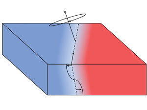
  $\hat {\boldsymbol {z}}\times \nabla _H b$. Typically, variations in the along-front direction occur over larger scales than cross-front variations and, hence, examples of fronts with no along-front variation are used to illustrate these results. A typical frontal set-up is shown in figure 1.

Figure 1. Typical non-dimensional frontal geometry showing a front with horizontal buoyancy gradient,  $\nabla _H b$, and buoyancy of
  $b = -1$ (resp.
  $b = 1$) on the low (resp. high) buoyancy side of the front. Top and bottom boundary conditions are applied at
  $z = \pm 1/2$. In this non-dimensional set-up the system is rotating with angular velocity
  $\delta \hat {\boldsymbol {y}}+\hat {\boldsymbol {z}}$.
If the system is independent of  $y$ – corresponding to a front aligned in the north–south direction – the non-traditional terms can be removed from (2.5) by replacing
  $p$ by
  $p+p_\delta$, where
  $p_\delta$ is defined using
 \begin{equation} \frac{\partial p_\delta}{\partial x} ={-}\delta w \quad \textrm{and} \quad \frac{\partial p_\delta}{\partial z} = \delta u. \end{equation}
This definition is consistent as it can be easily shown to satisfy mass conservation. The resulting system is equivalent to setting  $\delta = 0$ and, hence, non-traditional effects have no effect beyond the addition of an extra term in the pressure field.
3. Asymptotic expansion
To proceed, the parameters  $\delta$ and
  $Ro$ are assumed small with
  $\delta \gg Ro$. Taking
  $Ro \sim \delta ^2$, quantities may be expanded using an asymptotic expansion in
  $\delta$ by writing
 \begin{equation} \varphi = \varphi_0 + \delta \varphi_1 + \delta^2 \varphi_2 + \cdots \end{equation}
for some field  $\varphi$. Substituting expansions of this form into (2.5) gives a system of equations for each power of
  $\delta$. Typically, Ekman numbers lie in the range of
  $E \sim 0.01 - 1$ (Crowe & Taylor Reference Crowe and Taylor2018). However, it should be noted that even for
  $E \ll 1$, fields may be significantly modified within the top and bottom Ekman layers (of depth
  $O(\sqrt {E})$) so
  $E$ is taken to be an
  $O(1)$ quantity throughout. Mathematically, this may be seen as retaining the highest vertical derivatives in order to enforce the top and bottom boundary conditions.
Before proceeding with the analysis it is worth discussing the time derivative terms in (2.5). Unlike the TTW solutions of Crowe & Taylor (Reference Crowe and Taylor2018, Reference Crowe and Taylor2019b), steady solutions to order  $O(Ro)$ do not exist; this unsteadiness results from the generation of depth-averaged vorticity by non-traditional effects.
3.1. Generation of vorticity by non-traditional effects
Neglecting terms of order  $O(\delta ^2)$ from (2.5) and depth averaging (2.5a), (2.5b) and (2.5e) gives
 $$\begin{gather} \frac{\partial \bar{u}}{\partial t}+\delta \bar{w} - \bar{v} ={-}\frac{\partial \bar{p}}{\partial x}, \end{gather}$$
 $$\begin{gather}\frac{\partial \bar{v}}{\partial t}+ \bar{u} ={-}\frac{\partial \bar{p}}{\partial y}, \end{gather}$$
 $$\begin{gather}\frac{\partial \bar{u}}{\partial x}+\frac{\partial \bar{v}}{\partial y} = 0, \end{gather}$$
which may be combined to give
 \begin{equation} \frac{\partial }{\partial t}\left(\frac{\partial \bar{v}}{\partial x}-\frac{\partial \bar{u}}{\partial y}\right) = \delta \frac{\partial \bar{w}}{\partial y}. \end{equation}
Equation (3.3) states that the non-traditional component of the Coriolis force acts to generate vorticity over long times,  $t \sim O(1/\delta )$. This suggests the inclusion of a second time scale,
  $T = \delta t$, corresponding to this vorticity generation. Using a multiple scales approach the time derivative may be expanded as
 \begin{equation} \frac{\partial }{\partial t} \to \frac{\partial }{\partial t}+\delta\frac{\partial }{\partial T}, \end{equation}
where now the  ${\partial }/{\partial t}$ term corresponds to transient inertial oscillations resulting from an unbalanced initial condition. From Crowe & Taylor (Reference Crowe and Taylor2018), a longer time scale on the order of
  $t \sim O(\delta ^4)$ is also expected to be important. This slow scale corresponds to shear dispersive spreading of the front and will be discussed in § 3.6.
From now on transient oscillations are neglected by setting the fast time derivative,  ${\partial }/{\partial t}$, to zero. Therefore, the system is assumed to be balanced over the inertial time scale
  $t$ and only the slow evolution is considered.
3.2. The  $O(1)$ solution

At leading order in  $\delta$ (2.5) gives
 $$\begin{gather} - v_0 ={-}\frac{\partial p_0}{\partial x}+E\frac{\partial ^2u_0}{\partial z^2}, \end{gather}$$
 $$\begin{gather}u_0 ={-}\frac{\partial p_0}{\partial y}+E\frac{\partial ^2v_0}{\partial z^2}, \end{gather}$$
 $$\begin{gather}0 =\frac{E}{Pr}\frac{\partial ^2b_0}{\partial z^2}, \end{gather}$$
 $$\begin{gather}0 ={-}\frac{\partial p_0}{\partial z}+b_0, \end{gather}$$
 $$\begin{gather}\frac{\partial u_0}{\partial x}+\frac{\partial v_0}{\partial y}+\frac{\partial w_0}{\partial z} = 0, \end{gather}$$
corresponding to the leading-order (in  $Ro$) TTW system of Crowe & Taylor (Reference Crowe and Taylor2018). The leading-order buoyancy equation may now be solved for
 \begin{equation} b_0 = b_0(x,y,T); \end{equation}
hence, the layer is vertically well mixed to leading order in  $\delta$. The leading-order pressure may now be solved as
 \begin{equation} p_0 = \bar{p}_0+z b_0, \end{equation}
where  $\bar {p}_0$ balances the depth-averaged component of velocity through geostrophic balance. This depth-averaged flow may be represented as a streamfunction by
 \begin{equation} \bar{u}_0 ={-}\frac{\partial \psi_0}{\partial y},\quad \bar{v}_0 = \frac{\partial \psi_0}{\partial x}, \end{equation}
where  $\psi _0 = \bar {p}_0$ so the depth-averaged pressure acts as a streamfunction for this horizontal flow. The depth-dependent velocity fields,
  $(u_0',v_0',w_0)$, may be calculated (see Crowe & Taylor Reference Crowe and Taylor2018) by solving a fourth-order linear system to obtain solution
 $$\begin{gather} u_0' ={-}\sqrt{E}\left[K''(\zeta)\frac{\partial b_0}{\partial x}-K(\zeta)\frac{\partial b_0}{\partial y}\right], \end{gather}$$
 $$\begin{gather}v_0' ={-}\sqrt{E}\left[K(\zeta)\frac{\partial b_0}{\partial x}+K''(\zeta)\frac{\partial b_0}{\partial y}\right], \end{gather}$$
 $$\begin{gather}w_0 =E\, K'(\zeta) \nabla_H^2 b_0, \end{gather}$$
where  $\zeta = z/\sqrt {E}$ and
  $K(\zeta )$ is an
  $E$ dependent vertical structure function satisfying
 \begin{equation} \begin{cases} K^{(4)}(\zeta)+K(\zeta)+\zeta = 0 & \textrm{for}\ \zeta \in[-\zeta_0,\zeta_0],\\ K'(\zeta) = 0 & \textrm{at}\ \zeta ={\pm} \zeta_0,\\ K'''(\zeta) = 0 & \textrm{at}\ \zeta ={\pm} \zeta_0, \end{cases} \end{equation}
where  $\zeta _0 = 1/(2\sqrt {E})$ is the value of
  $|\zeta |$ on the top and bottom surfaces. Note that primes (
 $'$) on
  $K$ are taken to mean derivatives with respect to
  $\zeta$ rather than deviations from a vertical average as used elsewhere. The full solution for
  $K(\zeta )$ is given by
  $K_0(\zeta )$ in Appendix A of Crowe & Taylor (Reference Crowe and Taylor2018). For
  $E \ll 1$, it can be shown that
  $K(\zeta )\sim -\zeta$ and, hence, thermal wind balance holds outside of thin boundary layers of width
  $O(\sqrt {E})$ near the top and bottom boundaries.
3.3. The $O(\delta )$ solution

At order  $O(\delta )$ (2.5) gives
 $$\begin{gather} \frac{\partial u_0}{\partial T}+w_0 - v_1 ={-}\frac{\partial p_1}{\partial x}+E\frac{\partial ^2u_1}{\partial z^2}, \end{gather}$$
 $$\begin{gather}\frac{\partial v_0}{\partial T}+ u_1 ={-}\frac{\partial p_1}{\partial y}+E\frac{\partial ^2v_1}{\partial z^2}, \end{gather}$$
 $$\begin{gather}\frac{\partial b_0}{\partial T}=\frac{E}{Pr}\frac{\partial ^2b_1}{\partial z^2}, \end{gather}$$
 $$\begin{gather}- u_0 ={-}\frac{\partial p_1}{\partial z}+b_1, \end{gather}$$
 $$\begin{gather}\frac{\partial u_1}{\partial x}+\frac{\partial v_1}{\partial y}+\frac{\partial w_1}{\partial z} = 0. \end{gather}$$
It can be shown that the only solutions satisfying (3.11c) along with no-flux boundary conditions are
 \begin{equation} \frac{\partial b_0}{\partial T} = 0 \quad \textrm{and} \quad b_1 = b_1(x,y,T). \end{equation}
Therefore,  $b_0$ does not change over the time scale
  $t = O(1/\delta )$ and the buoyancy is also depth independent to
  $O(\delta )$. The pressure may now be calculated using (3.9a) and (3.11d) as
 \begin{align} p_1 &= \bar{p}_1+(b_1 + \bar{u}_0) z -E \left[\left(K'(\zeta)-\frac{K(\zeta_0)}{\zeta_0}\right) \frac{\partial b_0}{\partial x}\right.\nonumber\\ &\quad \left.+\left(K'''(\zeta)-\frac{K''(\zeta_0)}{\zeta_0} +\frac{\zeta^2}{2}-\frac{\zeta_0^2}{6}\right)\frac{\partial b_0}{\partial y}\right], \end{align}
where the final term arises from the integral of  $u_0'$ and has been set to be depth independent.
3.3.1. The depth-averaged system
From (3.11a), (3.11b), and (3.11e), the depth-averaged velocity and pressure satisfy
 $$\begin{gather} \frac{\partial \bar{u}_0}{\partial T}+ \bar{w}_0 - \bar{v}_1 ={-}\frac{\partial \bar{p}_1}{\partial x}, \end{gather}$$
 $$\begin{gather}\frac{\partial \bar{v}_0}{\partial T}+ \bar{u}_1 ={-}\frac{\partial \bar{p}_1}{\partial y}, \end{gather}$$
 $$\begin{gather}\frac{\partial \bar{u}_1}{\partial x}+\frac{\partial \bar{v}_1}{\partial y} = 0, \end{gather}$$
which may be combined to give
 \begin{equation} \frac{\partial }{\partial T}\left(\frac{\partial \bar{v}_0}{\partial x}-\frac{\partial \bar{u}_0}{\partial y}\right) = \frac{\partial \bar{w}_0}{\partial y} \ \implies \ \frac{\partial }{\partial T}\nabla^2 \psi_0 = \frac{\partial \bar{w}_0}{\partial y}, \end{equation}
which describes the generation of depth-averaged vorticity. Substituting for  $\bar {w}_0$ gives that
 \begin{equation} \frac{\partial \psi_0}{\partial T} = 2 \sqrt{E^{3}} K(\zeta_0) \frac{\partial b_0}{\partial y} \ \implies \ \psi_0 = \varPsi_0 + 2\sqrt{E^{3}} K(\zeta_0) \frac{\partial b_0}{\partial y} T, \end{equation}
where  $\varPsi _0 = \varPsi _0(x,y)$ is the value of
  $\psi _0$ at
  $T = 0$. The depth-averaged geostrophic flow can now be determined from
  $\psi _0$. From (3.14c), the
  $O(\delta )$ depth-averaged flow may now be written as
 \begin{equation} \bar{u}_1 ={-}\frac{\partial \psi_1}{\partial y},\quad \bar{v}_1 = \frac{\partial \psi_1}{\partial x}, \end{equation}
where, by (3.14a) and (3.14b),  $\psi _1$ is related to
  $\bar {p}_1$ through
 \begin{equation} \bar{p}_1 = \psi_1 - 2\sqrt{E^{3}} K(\zeta_0) \frac{\partial b_0}{\partial x}. \end{equation}
To determine the evolution of  $\psi _1$ it is necessary to consider the
  $O(\delta ^2)$ system.
3.3.2. The depth-dependent system
The depth-dependent quantities may now be considered by subtracting the depth-averaged horizontal momentum equations in (3.14) from (3.11a) and (3.11b) to obtain
 $$\begin{gather} w_0' - v_1' ={-}\frac{\partial p_1'}{\partial x}+E\frac{\partial ^2u_1'}{\partial z^2}, \end{gather}$$
 $$\begin{gather}u_1' ={-}\frac{\partial p_1'}{\partial y}+E\frac{\partial ^2v_1'}{\partial z^2}, \end{gather}$$
where the time derivative terms vanish as  $(u_0',v_0')$ does not depend on
  $T$. Substituting for
  $w_0'$ using (3.9c) and
  $p_1'$ using (3.13), this system may be solved (see Appendix A) for solution
 $$\begin{gather} u_1'={-}\sqrt{E}\left[K''(\zeta)\frac{\partial }{\partial x}-K(\zeta)\frac{\partial }{\partial y}\right]\left(b_1-\frac{\partial \psi_0}{\partial y}\right) +E\frac{\partial }{\partial y}\left[A(\zeta)\frac{\partial b_0}{\partial x}-B(\zeta)\frac{\partial b_0}{\partial y}\right], \end{gather}$$
 $$\begin{gather}v_1'={-}\sqrt{E}\left[K(\zeta)\frac{\partial }{\partial x}+K''(\zeta)\frac{\partial }{\partial y}\right]\left(b_1-\frac{\partial \psi_0}{\partial y}\right) +E\frac{\partial }{\partial y}\left[B(\zeta)\frac{\partial b_0}{\partial x}+A(\zeta)\frac{\partial b_0}{\partial y}\right]. \end{gather}$$
Finally,  $w_1$ may be calculated using (3.11e) as
 \begin{equation} w_1 = E K'(\zeta) \nabla_H^2 \left(b_1 - \frac{\partial \psi_0}{\partial y} \right) - \sqrt{E^3} C(\zeta) \nabla_H^2 \frac{\partial b_0}{\partial y}, \end{equation}
where  $C(\zeta )$ is the integral of
  $A(\zeta )$. The functions
  $A$,
$A$,  $B$ and
  $C$ are complicated functions of
  $\zeta$,
  $K(\zeta )$ and
  $\zeta _0$ and are given in Appendix B.
3.4. The $O(\delta ^2)$ solution

In Crowe & Taylor (Reference Crowe and Taylor2018) it was shown that an  $O(Ro)$ stratification is induced and maintained by an advection–diffusion balance in the buoyancy equation. Here this effect is expected to appear at orders
  $O(\delta ^2) = O(Ro)$ and
  $O(\delta ^3)$ and the
  $O(\delta ^2)$ system is considered first.
3.4.1. The buoyancy field
Since it has been assumed that  $Ro = O(\delta ^2)$, it is convenient to define
  $Ro = \mathcal {R}\, \delta ^2$, where
  $\mathcal {R}$ is an
  $O(1)$ number. The
  $O(\delta ^2)$ buoyancy equation is
 \begin{equation} \frac{\partial b_1}{\partial T} + \mathcal{R} \left(u_0\frac{\partial b_0}{\partial x}+v_0\frac{\partial b_0}{\partial y}\right) = \frac{E}{Pr} \frac{\partial ^2 b_2}{\partial z^2}, \end{equation}
and noting that  $b_1$ is depth independent, (3.22) may be depth averaged to obtain
 \begin{equation} \frac{\partial b_1}{\partial T} + \mathcal{R} J(\psi_0,b_0) = 0, \end{equation}
where  $J(\phi ,\varphi ) = (\partial _x \phi )(\partial _y \varphi ) - (\partial _y \phi )(\partial _x \varphi )$ is the Jacobian derivative. Substituting for
  $\psi _0$ gives
 \begin{equation} b_1 ={-}\mathcal{R} \left[ J(\varPsi_0,b_0)T + \sqrt{E^3} K(\zeta_0) J\left(\frac{\partial b_0}{\partial y},b_0\right) T^2\right], \end{equation}
assuming that  $b_1 = 0$ at
  $T=0$.
Subtracting (3.23) from (3.22) gives
 \begin{equation} \mathcal{R}\left(u_0'\frac{\partial b_0}{\partial x}+v_0'\frac{\partial b_0}{\partial y}\right) = \frac{E}{Pr} \frac{\partial ^2 b_2}{\partial z^2}. \end{equation}
This equation was considered in Crowe & Taylor (Reference Crowe and Taylor2018) and describes the restratification of the front by the TTW circulation. The solution is
 \begin{equation} b_2 = \bar{b}_2(x,y,T) - \mathcal{R}\,Pr\, \sqrt{E}\, K(\zeta) |\nabla_H b_0|^2. \end{equation}
3.4.2. The streamfunction for the depth-averaged flow
Depth-dependent velocity components of order higher than  $O(\delta )$ are not required in the subsequent calculations. However, higher-order components of
  $\psi$ are required to determine the higher-order depth-averaged buoyancy terms and may be determined by considering the vertical vorticity.
The depth-averaged vertical vorticity equation may be derived by cross-differentiating (2.5a) and (2.5b) and depth averaging to obtain
 \begin{equation} \delta \frac{\partial \bar{\eta}}{\partial T} + Ro\, \nabla_H \boldsymbol{\cdot} \left[ \overline{\boldsymbol{u}_H \eta} - \overline{\boldsymbol\omega_H w} \right] = \delta \frac{\partial \bar{w}}{\partial y}. \end{equation}
Here  $\boldsymbol {u}_H = (u,v,0)$ is the horizontal velocity,
  $\eta = {\partial v}/{\partial x}-{\partial u}/{\partial y}$ is the vertical vorticity and
 \begin{equation} \boldsymbol\omega_H =\begin{pmatrix} \displaystyle \frac{\partial w}{\partial y}-\frac{\partial v}{\partial z}\\ \displaystyle \frac{\partial u}{\partial z}-\frac{\partial w}{\partial x}\\ 0 \end{pmatrix} \end{equation}
is the horizontal vorticity. At  $O(\delta ^2)$ (3.27) gives
 \begin{equation} \frac{\partial \nabla_H^2\psi_1}{\partial T}+\mathcal{R}\, J[\psi_0,\nabla_H^2 \psi_0] = \mathcal{R} \nabla_H \boldsymbol{\cdot} [ -\overline{\boldsymbol{u}_{H0}' \eta_0'} + \overline{\boldsymbol\omega_{H0} w_0}] + \frac{\partial \bar{w}_1}{\partial y}, \end{equation}
where the flux terms can be expressed in terms of  $b_0$ to give
 \begin{equation} \frac{\partial \nabla_H^2\psi_1}{\partial T}+\mathcal{R} J[\psi_0,\nabla_H^2 \psi_0] = \mathcal{R} \nabla_H \boldsymbol{\cdot} [{\boldsymbol{\mathsf{P}}}\boldsymbol{\cdot} \nabla_H b_0 \nabla_H^2 b_0] + \frac{\partial \bar{w}_1}{\partial y} \end{equation}
for
 \begin{equation} {\boldsymbol{\mathsf{P}}} = E \begin{pmatrix} 2\overline{K'^2} & \overline{K^2}-\overline{K''^2} \\ \overline{K''^2}-\overline{K^2} & 2\overline{K'^2} \end{pmatrix}. \end{equation}
The flux term in (3.30) corresponds to both the generation of vorticity due to vortex stretching and the horizontal transport of vorticity due to a correlation between the vertically sheared profiles for the horizontal velocity and the vertical vorticity. Over time scales longer than  $T$, these terms have been shown to generate along-front jets (Crowe & Taylor Reference Crowe and Taylor2019b) and play a role in baroclinic instability (Crowe & Taylor Reference Crowe and Taylor2019a). Vorticity is also generated by the non-traditional component of the Coriolis force through the
  $y$ variations in
  $\bar {w}_1$, as discussed in § 3.1.
Equation (3.30) may be solved for  $\nabla _H^2\psi _1$ by a simple integration in
  $T$. However, solving for
  $\psi _1$ requires inverting the Laplacian operator so it is not possible to present a simple analytic solution. Solutions for (3.30) could be easily found numerically for given fields
  $b_0$,
  $\psi _0$ and
  $b_1$.
3.5. The $O(\delta ^3)$ solution

Now the order  $O(\delta ^3)$ balance is considered to determine the stratification maintained by the
  $O(\delta )$ velocity component. The
  $O(\delta ^3)$ vorticity equation will not be examined though it may be derived from (3.27) similarly to (3.30). The buoyancy equation is
 \begin{equation} \frac{\partial b_2}{\partial T} + \mathcal{R} \left( u_1 \frac{\partial b_0}{\partial x}+v_1\frac{\partial b_0}{\partial y} + u_0\frac{\partial b_1}{\partial x}+v_0\frac{\partial b_1}{\partial y}\right) = \frac{E}{Pr} \frac{\partial ^2 b_3}{\partial z^2}, \end{equation}
which may be depth averaged to obtain
 \begin{equation} \frac{\partial \bar{b}_2}{\partial T} + \mathcal{R} [ J(\psi_1,b_0) + J(\psi_0,b_1) ] = 0. \end{equation}
This equation may be solved using the expression for  $\psi _1$ if required. Since the depth-averaged buoyancy is known to the first two orders in
  $\delta$ and it is not possible to find a simple analytic expression for
  $\psi _1$, expressions for
  $\bar {b}$ are not calculated explicitly at
  $O(\delta ^2)$ or higher. Instead, the focus is on determining the vertical structure of
  $b$, denoted
  $b'$, to the lowest two orders. Since the lowest-order term in
  $b'$ is
  $b'_2$ (see (3.26)), the next order term,
  $b_3'$, must also be determined.
Subtracting (3.33) from (3.32) and noting that  ${\partial b_2'}/{\partial T} = 0$ gives the equation for the depth-dependent buoyancy
 \begin{equation} \mathcal{R} \left( u_1' \frac{\partial b_0}{\partial x} + v_1' \frac{\partial b_0}{\partial y} + u_0' \frac{\partial b_1}{\partial x} + v_0' \frac{\partial b_1}{\partial y} \right) = \frac{E}{Pr}\frac{\partial ^2 b_3}{\partial z^2}, \end{equation}
with solution
 \begin{align} b_3 &= \bar{b}_3(x,y,T) + \mathcal{R}\,Pr \left[ E \left( \frac{D_1(\zeta)}{2} \frac{\partial }{\partial y} |\nabla_H b_0|^2 + D_2(\zeta) J\left[ \frac{\partial b_0}{\partial y},b_0\right] \right) \right. \nonumber\\ &\quad + \sqrt{E} \left( K(\zeta) \left( \nabla_H \frac{\partial \psi_0}{\partial y} \cdot \nabla_H b_0 - 2 \nabla_H b_0 \cdot \nabla_H b_1 \right)\right. \nonumber\\ &\quad \left.\left. -\left( K''(\zeta)+\frac{\zeta^3}{6}-\frac{\zeta\zeta_0^2}{2} \right) J\left[\frac{\partial \psi_0}{\partial y},b_0\right]\right)\right], \end{align}
where the vertical structure functions  $D_1(\zeta )$ and
  $D_2(\zeta )$ are given in Appendix B. The term
  $\bar {b}_4$ can be determined by depth averaging the
  $O(\delta ^5)$ buoyancy equation, as noted above, this calculation is not done here.
3.6. Higher-order terms and shear dispersive spreading
The asymptotic approach may be continued as above to  $O(\delta ^4)$ and higher. However, from Crowe & Taylor (Reference Crowe and Taylor2018, Reference Crowe and Taylor2019b), slow frontal spreading is expected due to a buoyancy flux resulting from the correlation between the leading-order velocity and the
  $O(\delta ^2)$ stratification,
  $\overline {\boldsymbol {u}_{H0}' b_2'}$. This spreading is due to shear dispersion and was found to appear in the equations at
  $O(Ro^2) = O(\delta ^4)$ and occur over a time scale of
  $t = O(1/Ro^2) = O(1/\delta ^4)$. Similarly, the flux terms
  $\overline {\boldsymbol {u}_{H1}' b_2'}$ and
  $\overline {\boldsymbol {u}_{H0}' b_3'}$ resulting from non-traditional effects might be expected to drive some buoyancy change at
  $O(\delta ^5)$. Therefore, new time scales are introduced to examine the effects of this shear dispersion.
The time scale  $T = \delta t$ was shown in § 3.1 to be the time scale over which an
  $O(1)$ amount of depth-averaged vorticity is generated by non-traditional effects. Over time scales longer than
  $T$, many of the terms in
  $\bar {b}$ and
  $\psi$ demonstrate secular growth and as such it is necessary to introduce additional slow time scales corresponding to this slow frontal spreading. This is done by equating the size of the time derivative of the leading-order buoyancy,
  $b_0$, with the shear dispersion terms
 \begin{equation} \frac{\partial b_0}{\partial t} \sim \delta^4 \mathcal{R} \nabla_H \boldsymbol{\cdot} [ \overline{\boldsymbol{u}_{H0}' b_2'} ] \quad \textrm{and} \quad \frac{\partial b_0}{\partial t} \sim \delta^5 \mathcal{R} \nabla_H \boldsymbol{\cdot} [ \overline{\boldsymbol{u}_{H1}' b_2'} + \overline{\boldsymbol{u}_{H0}' b_3'}], \end{equation}
to get two time scales,  $T_4 = \delta ^4 t$ and
  $T_5 = \delta ^5 t$, and letting
  $b_0$ depend on
  $T_4$ and
  $T_5$. Here
  $T_4$ corresponds to the slow spreading time scale from Crowe & Taylor (Reference Crowe and Taylor2018) while
  $T_5$ corresponds to a longer time scale on which the evolution of depth-averaged buoyancy occurs due to non-traditional effects. Determining a closed system in full generality requires knowing how
  $\psi$ evolves over the slow scales
  $T_4$ and
  $T_5$ which requires examining high-order equations for the depth-averaged vorticity (Crowe & Taylor Reference Crowe and Taylor2019a,Reference Crowe and Taylorb). Instead, the simplifying assumption of a straight front is made. Under this assumption, the
  $\psi$ dependent terms vanish and equations purely in terms of
  $b_0$ are recovered as
 \begin{equation} \frac{\partial b_0}{\partial T_4} = \mathcal{R}^2\,Pr\, \nabla_H \cdot [ {\boldsymbol{\mathsf{Q}}} \boldsymbol{\cdot} \nabla_H b_0 |\nabla_H b_0|^2], \end{equation}
and
 \begin{equation} \frac{\partial b_0}{\partial T_5} = \mathcal{R}^2\,Pr\, \nabla_H \cdot \left[ {\boldsymbol{\mathsf{R}}}_1 \boldsymbol{\cdot} \frac{\partial \nabla_H b_0}{\partial y} |\nabla_H b_0|^2 + {\boldsymbol{\mathsf{R}}}_2 \boldsymbol{\cdot} \nabla_H b_0 \frac{\partial }{\partial y}|\nabla_H b_0|^2\right], \end{equation}
where
 \begin{equation} {\boldsymbol{\mathsf{Q}}}(E) = E \begin{pmatrix} \overline{K'^2} & \overline{K^2} \\ -\overline{K^2} & \overline{K'^2} \end{pmatrix}, \end{equation}
and
 \begin{equation} {\boldsymbol{\mathsf{R}}}_1(E) = E\sqrt{E} \begin{pmatrix} \overline{AK} & -\overline{BK} \\ \overline{BK} & \overline{AK} \end{pmatrix}, \quad {\boldsymbol{\mathsf{R}}}_2(E) = \frac{E\sqrt{E}}{2} \begin{pmatrix} \overline{AK} & -\overline{D_1K} \\ \overline{D_1K} & \overline{AK} \end{pmatrix}. \end{equation}
Equation (3.37) is identical to the result derived in Crowe & Taylor (Reference Crowe and Taylor2018) and describes the spreading of a front due to a horizontal buoyancy flux resulting from the correlation between the induced stratification and the cross-front flow. Equation (3.38) similarly describes a horizontal buoyancy flux, with terms arising from the non-traditional corrections to the stratification and cross-front flow.
It is worth noting that over long time scales the generation of significant background vorticity is expected, both by non-traditional effects as discussed in § 3.1 and due to the correlation between along-front and cross-front velocity fields as shown in (3.30) and discussed in Crowe & Taylor (Reference Crowe and Taylor2019b). These correlation terms appear as a consequence of vertical mixing driving a cross-front flow and do not appear in the limit of  $E \to 0$. The generated vorticity manifests as along-front jets and can become large enough to significantly modify the absolute vorticity of the system resulting in a modification of the TTW velocity solution and, hence, a modified stratification and frontal spreading. Additionally, frontal systems are susceptible to baroclinic instability (Stone Reference Stone1966; Crowe & Taylor Reference Crowe and Taylor2019a) which may lead to a breakdown of the straight front assumption.
4. Summary of solution
Here the solution of § 3 is summarised and results are presented and discussed for a simple frontal geometry.
4.1. The velocity fields
Correct to  $O(\delta )$, the velocity fields are given by
 \begin{align} \boldsymbol{u}_H &={-}\boldsymbol{\nabla}\times[ (\psi_0+\delta\psi_1)\hat{\boldsymbol{z}}]-\sqrt{E} {\boldsymbol{\mathsf{K}}}\boldsymbol{\cdot} \nabla_H \left(b_0+\delta\,b_1 - \delta\frac{\partial \psi_0}{\partial y}\right)\nonumber\\ &\quad + \delta E {\boldsymbol{\mathsf{A}}}\boldsymbol{\cdot} \nabla_H\frac{\partial b_0}{\partial y} + O(\delta^2), \end{align}
and
 \begin{equation} w = E K'(\zeta) \nabla_H^2 \left(b_0+\delta\,b_1 - \delta\frac{\partial \psi_0}{\partial y}\right) - \delta \sqrt{E^3} C(\zeta) \nabla_H^2 \frac{\partial b_0}{\partial y} +O(\delta^2), \end{equation}
where
 \begin{equation} {\boldsymbol{\mathsf{K}}}(\zeta) = \begin{pmatrix} K''(\zeta) & -K(\zeta) \\ K(\zeta) & K''(\zeta) \end{pmatrix} \quad \textrm{and} \quad {\boldsymbol{\mathsf{A}}}(\zeta) = \begin{pmatrix} A(\zeta) & -B(\zeta) \\ B(\zeta) & A(\zeta) \end{pmatrix}. \end{equation}
The depth-averaged velocity is described by a streamfunction where
 \begin{equation} \psi_0 = \varPsi_0 + 2\sqrt{E^{3}} \delta t K(\zeta_0) \frac{\partial b_0}{\partial y}, \end{equation}
for some initial streamfunction  $\psi _0 = \varPsi _0$ at
  $t = 0$. It should be noted that
  $t = O(1/\delta )$ so all terms here are leading order. The
  $O(\delta )$ streamfunction component,
  $\psi _1$, satisfies (3.30).
The leading-order flow can be split into components in the cross-front direction (described by the diagonal terms in  ${\boldsymbol{\mathsf{K}}}$) and along-front direction (described by the off-diagonal terms in
  ${\boldsymbol{\mathsf{K}}}$). However, the
  $O(\delta )$ terms are aligned relative to gradients of the north–south (
 $y$) derivatives of
  $b_0$ and
  $\psi _0$ which do not necessarily correspond to the direction of
  $\nabla _H b_0$.
Two special cases are  $b_0 = b_0(x)$ and
  $b_0 = b_0(y)$. The case of
  $b_0 = b_0(x)$ describes a front with the along-front direction aligned north–south. In this case all
  $y$ derivatives can be neglected and the non-traditional terms have no effect on the front as discussed in § 2. Conversely,
  $b_0 = b_0(y)$ describes a front with the along-front direction aligned east–west. In this case non-traditional effects are maximised and the gradients of
  $b_0$ are aligned with the gradients of
  ${\partial b_0}/{\partial y}$ so the horizontal velocity terms driven by the non-traditional rotation can be easily split into cross-front and along-front components similarly to the leading-order flow.
4.2. The buoyancy field
The buoyancy field can be split into depth-averaged and depth-dependent components. Correct to the lowest two orders in  $\delta$ the solutions are
 \begin{equation} \bar{b} = b_0+\delta b_1 +O(\delta^2) = b_0 -Ro \,t J\left[\varPsi_0 + \sqrt{E^3} \delta t K(\zeta_0)\frac{\partial b_0}{\partial y},b_0\right] + O(\delta^2), \end{equation}
where  $Ro\,t = O(\delta )$. The depth-dependent buoyancy is given by
 \begin{align} b' &= Ro\,Pr\, \sqrt{E} \left[ \left(- K(\zeta) +\delta \sqrt{E} \frac{D_1(\zeta)}{2} \frac{\partial }{\partial y} \right) |\nabla_H b_0|^2 + \delta \left( \sqrt{E} D_2(\zeta) J\left[ \frac{\partial b_0}{\partial y},b_0 \right]\right.\right. \nonumber\\ &\quad + \left.\left. K(\zeta) \nabla_H\left( \frac{\partial \psi_0}{\partial y} - 2 b_1 \right)\cdot\nabla_H b_0 -\left( K''(\zeta)+\frac{\zeta^3}{6}-\frac{\zeta\zeta_0^2}{2} \right) J\left[\frac{\partial \psi_0}{\partial y},b_0\right]\right)\right] \nonumber\\ &\quad + O(\delta^4). \end{align}
Similarly to the velocity fields, if  $b_0 = b_0(x)$ then the non-traditional rotation has no effect on the front and the solution reduces to the results of Crowe & Taylor (Reference Crowe and Taylor2018). From
  $b'$ the vertical buoyancy gradient,
  $N^2$, may be determined as
 \begin{align} N^2 &= \frac{\partial b'}{\partial z} = Ro\,Pr\left[ \left(- K'(\zeta) +\delta\,\sqrt{E} \frac{D_1'(\zeta)}{2} \frac{\partial }{\partial y} \right) |\nabla_H b_0|^2 + \delta \left( \sqrt{E} D_2'(\zeta)\, J\left[ \frac{\partial b_0}{\partial y},b_0\right] \right.\right. \nonumber\\ &\quad + \left.\left. K'(\zeta) \nabla_H\left( \frac{\partial \psi_0}{\partial y} - 2 b_1 \right)\cdot\nabla_H b_0 -\left( K'''(\zeta)+\frac{\zeta^2}{2}-\frac{\zeta_0^2}{2} \right) J\left[\frac{\partial \psi_0}{\partial y},b_0\right]\right)\right] \nonumber\\ &\quad + O(\delta^4). \end{align}
The horizontal buoyancy gradient may be similarly calculated using
 \begin{equation} M^2 = \nabla_H b = \nabla_H \bar{b} + \nabla_H b', \end{equation}
where the first term on the right-hand side is leading order and depth independent while the second term is order  $O(Ro)$ and depth dependent.
4.3. Frontal spreading and shear dispersion
Over very long times the front is expected to evolve through shear dispersion. Equations (3.37) and (3.38) may be combined to give
 \begin{equation} \frac{\partial b_0}{\partial t} = Ro^2\,Pr\, \nabla_H \cdot \left[ \left({\boldsymbol{\mathsf{Q}}} \boldsymbol{\cdot} \nabla_H b_0+\delta\,{\boldsymbol{\mathsf{R}}}_1 \boldsymbol{\cdot} \nabla_H \frac{\partial b_0}{\partial y} + \delta\,{\boldsymbol{\mathsf{R}}}_2 \boldsymbol{\cdot} \nabla_H b_0\, \frac{\partial }{\partial y}\right)|\nabla_H b_0|^2\right], \end{equation}
which is valid for a straight front provided the vorticity generated by non-traditional effects and vertical mixing is less than the background vorticity. Expressions for  ${\boldsymbol{\mathsf{Q}}}$,
  ${\boldsymbol{\mathsf{R}}}_1$ and
  ${\boldsymbol{\mathsf{R}}}_2$ are given in (3.39) and (3.40a,b). It should be noted that (4.9) reduces to the results of Crowe & Taylor (Reference Crowe and Taylor2018) for
  $b_0 = b_0(x)$, similarly to the results for velocity and buoyancy. If
  $b_0 = b_0(y)$ is an odd function of
  $y$, then solutions to (4.9) will remain odd in
  $y$ for all time for the case of
  $\delta = 0$. However, for
  $\delta \neq 0$, the addition of an extra
  $y$ derivative in the non-traditional correction terms leads to an asymmetry and, hence, different evolution on each side of the front.
5. A simple frontal geometry
To illustrate the results given in § 4, solutions are plotted for the simple case of
 \begin{equation} b_0 = \tanh y. \end{equation}
As noted in the previous section, this corresponds to a front with the along-front direction (here the  $x$ direction) aligned east–west so that non-traditional effects are maximised. From (4.5), it can be seen that
  $b_1 = 0$ since the Jacobian terms vanish. Similarly, higher-order depth-averaged buoyancy terms, such as
  $\bar {b}_2$ and
  $\bar {b}_3$, will evolve through advection by Jacobian terms so may also be set to zero. Therefore,
  $b_0$ may be taken to describe the full depth-averaged buoyancy.
5.1. Depth-independent jets
Taking the initial streamfunction of  $\varPsi _0 = 0$, the depth-averaged velocity is given by
 \begin{equation} \psi_0 = 2\sqrt{E^{3}} \delta t K(\zeta_0)\textrm{sech}^2 y \ \implies \ (\bar{u}_0,\bar{v}_0) = 4\sqrt{E^{3}} \delta t K(\zeta_0)(\textrm{sech}^2 y \tanh y,0), \end{equation}
corresponding to two jets running in opposite directions along the edges of the front. As expected, motion is confined to the frontal region. Since the Jacobian terms vanish for  $b_0 = b_0(y)$, (3.30) may be solved for
  $\psi _1$ as
 \begin{equation} \psi_1 = \mathcal{R}E \delta t \overline{K'^2}\left(\frac{\partial b_0}{\partial y}\right)^2 - 2\,E^3(\delta t)^2 [K(\zeta_0)]^2 \frac{\partial ^3b_0}{\partial y^3}. \end{equation}
The first term of  $\psi _1$ in (5.3) describes the vorticity generated by the correlation between the cross-front and along-front TTW velocities (Crowe & Taylor Reference Crowe and Taylor2019b), while the second term describes the generation of vorticity through the action of the non-traditional Coriolis force on the
  $O(\delta )$ vertical velocity. The streamfunction and along-front velocity of the depth-independent jets are shown in figure 2 correct to
  $O(\delta )$ as a function of
  $y$ for
  $E = 0.1$,
  $\delta = 0.2$,
  $\delta \,t = 1$ and
  $\mathcal {R} = 1$. These jets grow with time and are expected to become large for
  $T\gg 1$.

Figure 2. The streamfunction (a) and velocity (b) of the along-front jets. Solutions are shown correct to  $O(\delta )$ for
  $E = 0.1$,
  $\delta = 0.2$,
  $\delta \,t = 1$ and
  $\mathcal {R} = 1$.
5.2. Frontal circulation
For an  $x$ independent front, the cross-front velocity (
 $v$) and vertical velocity (
 $w$) satisfy the mass conservation equation
 \begin{equation} \frac{\partial v'}{\partial y} + \frac{\partial w}{\partial z} = 0, \end{equation}
and, hence, the circulation around the front in the  $y-z$ plane can be represented by a circulation streamfunction,
  $\phi$, defined using
 \begin{equation} v' = \frac{\partial \phi}{\partial z}, \quad w ={-}\frac{\partial \phi}{\partial y}. \end{equation}
Note that there is no depth-independent flow in the  $y$ direction as
  $\psi = \psi (y)$ so
  $v = v'$ here. The circulation components,
  $\phi _0$ and
  $\phi _1$, are given by
 \begin{equation} \phi_0 ={-}E K'(\zeta) \frac{\partial b_0}{\partial y}, \quad \phi_1 = \sqrt{E^3} C(\zeta) \frac{\partial ^2b_0}{\partial y^2} + E K'(\zeta)\frac{\partial ^2\psi_0}{\partial y^2}. \end{equation}
The two terms of  $\phi _1$ in (5.6a,b) each arise due to different components of the non-traditional Coriolis force. The horizontal component appears directly in the horizontal momentum balance resulting in the first term of (5.6a,b) while the vertical component drives the system out of hydrostatic balance, modifying the pressure field and giving the second term.
Figure 3 shows a comparison between the TTW solutions of Crowe & Taylor (Reference Crowe and Taylor2018) (corresponding to  $\delta = 0$) and the modified TTW solutions presented here with
  $\delta = 0.4$. Solutions are given correct to
  $O(\delta )$ using
  $\varphi = \varphi _0+\delta \,\varphi _1$ for a given field
  $\varphi$ and shown for
  $E = 0.01$ and
  $T = 1$. The TTW solution consists of a flow from the high buoyancy side of the front to the low buoyancy side near the top surface and the opposite on the bottom surface. This results in upwelling on the high buoyancy side and downwelling on the low buoyancy side resulting in a anti-clockwise net circulation (shown by positive
  $\phi$). This behaviour was discussed in Crowe & Taylor (Reference Crowe and Taylor2018) and is consistent with previous results and observations (Eliassen Reference Eliassen1962; Orlanski & Ross Reference Orlanski and Ross1977; McWilliams Reference McWilliams2017). Non-traditional effects act to tilt the circulation cell and drive a flow in the centre of the layer. This flow may lead to a topological change in the structure of the circulation with a streamline in figure 3(c) seen to split into two separate cells.

Figure 3. Comparison between the TTW and modified TTW solutions for  $E = 0.01$ and
  $T = 1$; (a)
  $\phi$ for
  $\delta = 0$, (b)
  $\phi$ for
  $\delta = 0.4$, (c)
  $v$ for
  $\delta = 0$, (d)
  $v$ for
  $\delta = 0.4$, (e)
  $w$ for
  $\delta = 0$ and (f)
  $w$ for
  $\delta = 0.4$. Solutions are shown correct to
  $O(\delta )$.
Figure 4 shows separately the two terms of  $\phi _1$ from (5.6a,b) for
  $E = 0.1$ and
  $T = 1$. The associated cross-front velocities are also shown. The first term consists of four counter-rotating cells resulting in regions of convergence near the top and bottom boundaries and acting to tilt the leading-order circulation cell. The second term consists of three counter-rotating cells and results from the along-front jets modifying the vertical pressure gradient away from hydrostatic balance. As these jets grow, the second term of
  $\phi _1$ grows linearly with time for
  $T = O(1)$. Over very long time scales, it is predicted that these jets can become large enough to modify the absolute vertical vorticity in the frontal region. Therefore, while small in figure 3(b), this circulation component may become large at late times leading to further topological changes in the structure of the frontal circulation.

Figure 4. (a) The first term of the  $O(\delta )$ circulation streamfunction component,
  $\phi _1$, from (5.6a,b). (b) The second term of
  $\phi _1$ from (5.6a,b). Panels (c) and (d) show the cross-front velocity (
 $v$) components associated with the streamfunction components shown in panels (a) and (b), respectively. Results are shown for
  $E = 0.1$ and
  $T = 1$.
Additionally, by depth integrating the vertical velocities corresponding to the two terms in (5.6a,b) the net vertical transport of fluid may be calculated. The first term depth averages to zero so does not correspond to any vertical transport, instead this term describes a tilting of the circulation cell as noted above. The second term does, however, have a non-zero depth average which suggests that the circulation cells in figure 4(b) may act to enhance the vertical exchange of tracers through the surface mixed layer.
The  $O(\delta )$ cross-front velocities shown in figure 4 contain regions of surface convergence. This velocity convergence can lead to a sharpening of surface buoyancy gradients resulting in frontogenesis (Hoskins Reference Hoskins1982; Shakespeare & Taylor Reference Shakespeare and Taylor2013) and, hence, non-traditional effects may be frontogenetic. The asymptotic framework used here assumes
  $Ro \ll 1$ so this model is not strictly valid for studying frontogenesis where the Rossby number is typically order
  $1$. However, for
  $Ro = O(1)$, the frontal sharpening predicted here will be an
  $O(\delta )$ effect, therefore, away from the equator, non-traditional effects are unlikely to be a dominant frontogenetic mechanism when compared with other mechanisms such as external strain, spontaneous adjustment and the secondary circulation induced by finite Rossby number effects (Hoskins & Bretherton Reference Hoskins and Bretherton1972; Blumen Reference Blumen2000; Gula et al. Reference Gula, Molemaker and McWilliams2014; McWilliams Reference McWilliams2017). Non-traditional frontogenesis may be relevant in a small region around the equator where
  $\delta \geq O(1)$, though, since TTW is unlikely to be the dominant balance in this region, it is not possible to draw any conclusions from this analysis.
5.3. The along-front flow
The depth-dependent along-front velocity components are given by
 \begin{equation} u_0' = \sqrt{E} K(\zeta) \frac{\partial b_0}{\partial y}, \quad u_1' ={-} E B(\zeta)\frac{\partial ^2b_0}{\partial y^2} -\sqrt{E} K(\zeta) \frac{\partial ^2\psi_0}{\partial y^2}, \end{equation}
where the two terms of  $u_1'$ arise from the modified horizontal momentum balance and the modified hydrostatic balance similarly to the terms of
  $\phi _1$ in (5.6a,b).
Figure 5 shows the depth-dependent along-front velocity correct to  $O(\delta )$ for the cases of
  $\delta = 0$ and
  $\delta = 0.4$ with
  $T = 1$. The along-front flow is dominated by a thermal wind shear modified by vertical mixing (Crowe & Taylor Reference Crowe and Taylor2018) and non-traditional effects are seen to be small. Therefore, the most significant effect of non-traditional rotation on the along-front flow is the development of the depth-independent jets shown in figure 2 though if the jets become large, significant modification of the depth-dependent flow may occur through the second term of (5.7a,b).

Figure 5. Comparison of the along-front velocities for the TTW and modified TTW systems showing (a)  $u'$ for
  $\delta = 0$ and (b)
  $u'$ for
  $\delta = 0.4$. Parameters are
  $E = 0.01$ and
  $T = 1$ and solutions are given correct to
  $O(\delta)$.
5.4. Buoyancy and stratification
As noted above, the depth-averaged buoyancy remains equal to  $b_0$ for the simple case of
  $b_0 = \tanh y$. However, the vertical structure of the buoyancy field and the associated stratification are determined by the frontal circulation so are still affected by non-traditional rotation. These terms appear at orders
  $O(\delta ^2)$ and
  $O(\delta ^3)$ and from (4.6) are given by
 \begin{equation} \left.\begin{gathered} b_2 ={-}\mathcal{R}\,Pr\sqrt{E} K(\zeta)\left(\frac{\partial b_0}{\partial y}\right)^2,\\ b_3 =\mathcal{R}\,Pr\left( E D_1(\zeta)\frac{\partial b_0}{\partial y}\frac{\partial ^2b_0}{\partial y^2} + \sqrt{E} K(\zeta) \frac{\partial b_0}{\partial y}\frac{\partial ^2\psi_0}{\partial y^2}\right). \end{gathered}\right\} \end{equation}
The lowest-order buoyancy term with vertical structure,  $b_2$, describes the stratification maintained by an advection–diffusion balance between the advection of buoyancy by the leading-order circulation,
  $\phi _0$, and the vertical mixing of buoyancy (Crowe & Taylor Reference Crowe and Taylor2018). A similar balance occurs at
  $O(\delta ^3)$ so the first (second) term of
  $b_3$ in (5.8) describes the stratification maintained by the first (second) term of
  $\phi _1$.
Figure 6 shows the depth-dependent buoyancy,  $b'$, and vertical stratification,
  $N^2 = {\partial b}/{\partial z}$, correct to
  $O(\delta ^3)$ for
  $E = 0.01$ and
  $T = 1$. Solutions are shown for
  $\delta = 0$ and
  $\delta = 0.4$. Since
  $b'$ and
  $N^2$ are linear in
  $Ro\,Pr$ through the factor of
  $\mathcal {R} \delta ^2\,Pr$, results are plotted for
  $b'/(Ro\,Pr)$ and
  $N^2/(Ro\,Pr)$ to remove this dependence. The advection–diffusion balance is seen to drive a stable restratification of the front and modification by non-traditional effects is small unless
  $\psi _0$ becomes large.

Figure 6. Comparison between the TTW and modified TTW solutions for  $E = 0.01$ and
  $T = 1$; (a)
  $b'/(Ro\,Pr)$ for
  $\delta = 0$, (b)
  $b'/(Ro\,Pr)$ for
  $\delta = 0.4$, (c)
  $N^2/(Ro\,Pr)$ for
  $\delta = 0$ and (d)
  $N^2/(Ro\,Pr)$ for
  $\delta = 0.4$. Solutions are shown correct to
  $O(\delta )$.
From (5.8), the order  $O(\delta ^3)$ horizontal buoyancy gradient may be calculated as
 \begin{equation} M^2_3 = \frac{\partial b_3}{\partial y} = \mathcal{R}\,Pr\left( E D_1(\zeta)\frac{\partial }{\partial y}\left[\frac{\partial b_0}{\partial y}\frac{\partial ^2b_0}{\partial y^2}\right] + \sqrt{E}\,K(\zeta) \frac{\partial }{\partial y}\left[\frac{\partial b_0}{\partial y}\frac{\partial ^2\psi_0}{\partial y^2}\right]\right). \end{equation}
The two terms of (5.9) are plotted in figure 7 for  $E = 0.01$,
  $\mathcal {R}\,Pr = 1$ and
  $T = 1$. Regions of positive horizontal buoyancy gradient are observed for both terms in
  $M_3^2$, these regions correspond to frontal sharpening due to the cross-front velocity convergence seen in figure 4.


5.5. Shear dispersive spreading
For  $b_0 = b_0(y)$, (4.9) becomes
 \begin{equation} \frac{\partial b_0}{\partial t} = Ro^2\,Pr\, \frac{\partial }{\partial y}\left[c_3 \left(\frac{\partial b_0}{\partial y}\right)^3+\delta\,c_4 \left(\frac{\partial b_0}{\partial y}\right)^2\frac{\partial ^2b_0}{\partial y^2}\right] \end{equation}
for
 \begin{equation} c_3(E) = E\,\overline{K'^2} \quad \textrm{and} \quad c_4(E) = 2 \sqrt{E^3}\,\overline{AK}. \end{equation}
This equation is derived using the  $\psi _0$ independent terms from
  $b'_3$ and
  $\boldsymbol {u}'_{H1}$ and corresponds to the case of weak vorticity generation,
  $\psi _0 = 0$. Over the long time scale of shear dispersive spreading,
  $t=O(1/\delta ^4)$, significant vorticity generation is expected. However, the case of
  $\psi _0 = 0$ is considered here to isolate the effect of the
  $\psi$ independent terms.
As  $\delta \to 0$, (5.10) reduces to the result of Crowe & Taylor (Reference Crowe and Taylor2018) where the front approaches a self-similar solution and spreads as
  $y \sim t^{1/4}$. This self-similar solution is odd in
  $y$, hence, the high buoyancy and low buoyancy sides evolve in the same way. However, the
  $c_4$ term breaks this
  $y$ symmetry due to an odd number of
  $y$ derivatives so both sides are expected to evolve differently for non-zero
  $\delta$. To test this prediction, (5.10) is solved numerically using the Dedalus framework (Burns et al. Reference Burns, Vasil, Oishi, Lecoanet and Brown2020). The units of time are rescaled such that
  $Ro^2Pr\,c_3 = 1$ leaving
  $r = \delta c_4/c_3$ as the only free parameter. Simulations are run for
  $r = 0$ and
  $r = 0.2$ and initialised using the profile
  $b_0(t = 0) = \tanh y$. Sixth-order hyperdiffusion with a hyperdiffusivity of
  $\nu _6 = 3\times 10^{-9}$ is included for numerical stability and simulations are run until
  $Ro^2Pr\,c_3 t = 10$ using a third-order implicit–explicit Runge–Kutta scheme and a domain of
  $y \in [-5,5]$ with
  $N_y = 256$ grid points.
Figure 8 shows the numerical solutions for  $b_0$ for
  $r = 0$ and
  $r = 0.2$ at a range of times. The difference between these two solutions is plotted in panel (b) allowing the expected asymmetry due to non-traditional effects to be observed. The effect of the non-traditional term is found to be small and of greatest importance near the frontal edges where the curvature,
  ${\partial ^2b_0}/{\partial y^2}$, is large. Therefore, it is expected that non-traditional effects will not play a significant role in the shear dispersive spreading of a front without the inclusion of strong vorticity generation.

Figure 8. (a) The buoyancy field,  $b_0$, from numerically solving (5.10). Solutions are calculated for
  $r = \delta c_4/c_3 = 0$ (red) and
  $r = 0.2$ (blue) and shown for
  $Ro^2Pr\,c_3 t \in [0, 2.5, 5, 7.5, 10]$ with steeper solutions corresponding to earlier times. (b) The difference in
  $b_0$ between the
  $r = 0$ results and the
  $r = 0.2$ results for the same time values as (a).
Over long times, a large amount of vorticity is expected to be generated by both vertical mixing (Crowe & Taylor Reference Crowe and Taylor2019b) and non-traditional effects. This vorticity manifests as depth-independent jets and can act to modify the total vorticity of the system. If this vorticity is sufficiently strong, local vorticity terms can appear in the leading-order TTW balance. These terms will modify the Coriolis force, resulting in a modified depth-dependent velocity and, hence, a modified circulation. Therefore, it is predicted that the generation of vorticity will play a more important role in the evolution of  $b_0$ than the
  $\psi _0$ independent circulation considered here. The effects of large
  $\psi _0$ could be considered using the approach of Crowe & Taylor (Reference Crowe and Taylor2019b); however, such solutions are expected to be complicated and provide no new insight into the problem so will not be considered here.
6. The finite Rossby number regime
Throughout we have taken  $Ro = O(\delta ^2)$. This assumption is predominantly for mathematical convenience as it results in linear equations for the velocity at the first two orders in
  $\delta$. However, frontal systems in which non-traditional effects are important are unlikely to have small Rossby numbers. Here, typical frontal parameters are discussed and numerical simulations are presented for parameters outside of the regime considered above.
6.1. Typical frontal parameters
The small parameter describing non-traditional effects is the ratio of the vertical and horizontal components of the rotation vector scaled by the aspect ratio and is given by
 \begin{equation} \delta = \frac{H}{L} \frac{1}{\tan \theta} \end{equation}
for latitude  $\theta$, layer depth
  $H$ and typical frontal width
  $L$. The requirement that
  $Ro = O(\delta ^2)$ therefore implies that
 \begin{equation} B \sim H \tilde{f}^2, \end{equation}
where  $B$ is the typical buoyancy difference across the front. Taking typical values of
  $\tilde {f} \approx 10^{-4} \ \textrm {s}^{-1}$ and
  $H = 100\ \textrm {m}$ gives a buoyancy difference which is much smaller than the typical values of
  $B\approx 10^{-4}\ \textrm {ms}^{-2}$. Therefore, for this asymptotic regime to hold, the frontal velocities and, hence, the Rossby number would have to be much smaller than would be expected physically.
To determine more physical values of the relevant parameters, note that non-traditional effects are most important in the tropical and subtropical regions where  $\tan \theta < 1$. Here, fronts with small horizontal scales,
  $L \sim 1 \ \textrm {km}$, may have order
  $1$ values of
  $\delta$; however, the Rossby number would also be order
  $1$ for these small-scale fronts. This case of
  $Ro = O(1)$ and
  $\delta = O(0.1 - 1)$ is likely to be the most physically relevant regime. Previous studies (Crowe & Taylor Reference Crowe and Taylor2019b) have noted that TTW balance can remain valid even for the case of finite Rossby numbers so numerical simulations are now performed to test if the phenomenon described above are relevant to this regime.
6.2. Numerical simulations for $Ro = 1$

Here, (2.5) is solved subject to no-stress and no-flux boundary conditions using the Dedalus package (Burns et al. Reference Burns, Vasil, Oishi, Lecoanet and Brown2020). These numerical simulations are two dimensional; the cross-front direction is taken to align with the  $y$ axis where non-traditional effects are maximised and
  ${\partial }/{\partial x}$ is set to zero. Fields are expanded in terms of a Fourier basis in the horizontal
  $(y)$ direction and a Chebyshev basis in the vertical
  $(z)$ direction and time stepped using a third-order implicit–explicit Runge–Kutta scheme. Horizontal mixing with a viscosity of
  $10^{-4}$ is included for numerical stability. Simulations are initialised using the
  $O(1)$ TTW solution for velocity and buoyancy given in § 4 for
  $b_0 = \tanh y$ and
  $\psi _0 = 0$.
Figure 9 shows numerical results for  $Ro = 0.1$,
  $\delta = 1$ and
  $E = 0.1$. Figure 9(a) shows the development of the along-front jets through the growth of the streamfunction of the depth-averaged flow,
  $\psi$, with time. These profiles for
  $\psi$ are consistent with the analytical predictions shown in figure 2(a), differing by less than
  $3\,\%$ from the theory despite the use of an order
  $1$ value of
  $\delta$ in an asymptotic expression that is known only to
  $O(\delta )$. Figure 9(b) shows the
  $O(\delta )$ component of the streamfunction of the frontal circulation,
  $\phi _1$, at
  $t = 2$. Here
  $\phi _1$ is calculated as the difference between the total value of
  $\phi$ and the value of
  $\phi _0$ calculated using (5.6a,b). Again the results are well described by the theory as the structure of these circulation cells can be seen to be a sum of the components shown in figures 4(a) and 4(b). The accuracy of the theoretical predictions for order
  $1$ values of
  $\delta$ suggests that the solutions of § 4 are valid, even outside of the asymptotic regime considered.

Figure 9. Results from a numerical simulation with  $(Ro,\delta ,E) = (0.1,1,0.1)$ showing (a) the streamfunction,
  $\psi$, describing the depth-averaged along-front flow and (b) the circulation component
  $\phi _1$ at
  $t = 2$.
Figure 10 shows numerical results for  $Ro = 1$,
  $\delta = 1$ and
  $E = 0.1$. Here, the effects of nonlinearity become significant and it is necessary to separate the effects of finite
  $Ro$ from the effects of finite
  $\delta$. This may be done by running another simulation with
  $(Ro,\delta ,E) = (1,0,0.2)$ and calculating the difference
 \begin{equation} \Delta \varphi = \varphi|_{\delta = 1} - \varphi|_{\delta = 0} \end{equation}
for some field  $\varphi$. Figure 10(a) shows the value of
  $\Delta \psi$ for a range of values of
  $t$. Similarly to the case of
  $Ro = 0.1$, the along-front flow is found to be well described by the theoretical predictions with a difference of around
  $4\,\%$ between
  $\Delta \psi$ and the prediction for
  $\psi _0+\delta \psi _1$. The difference in frontal circulation,
  $\Delta \phi$, is shown in figure 10(b). While qualitatively similar to theoretical predictions and the case of
  $Ro = 0.1$, the nonlinearity and non-traditional components appear to interact nonlinearly resulting in some deviation from the predictions. In particular, the centre of the middle circulation cell in figure 10(b) is seen to split in two. Nonetheless, even for cases far outside the asymptotic regime considered analytically, the effects of including non-traditional rotation appear to be qualitatively the same as discussed above, with the generation of along-front jets and a modification of the frontal circulation.

Figure 10. Results from a numerical simulation with  $(Ro,\delta ,E) = (1,1,0.1)$ showing (a) the difference in streamfunction,
  $\Delta \psi$, between the results for
  $\delta = 1$ and
  $\delta = 0$, and (b) the difference in frontal circulation,
  $\Delta \phi ,$ at
  $t = 2$.
7. Discussion and conclusions
Here the effects of the non-traditional component of rotation on a front in TTW balance have been considered. Solutions are calculated as a perturbation of the TTW solutions of Crowe & Taylor (Reference Crowe and Taylor2018, Reference Crowe and Taylor2019b) using an asymptotic approach. The magnitude of the non-traditional correction terms is found to depend strongly on the direction of the front. Fronts where the along-front direction is aligned north–south are found to be unaffected by the non-traditional rotation terms. Conversely, non-traditional effects are maximised for fronts aligned east–west.
A primary effect of the non-traditional rotation is the generation of vertical vorticity by the horizontal component of the non-traditional Coriolis force,  $\tilde {f}w$. This vorticity is generated in regions of strong vertical velocity and manifests as along-front jets. Over time scales of
  $t \sim 1/(\delta f)$ strong vorticity generation is expected, resulting in a modification of the total vertical vorticity of the system once the generated vorticity is of similar magnitude to the planetary vorticity,
  $f$. In this case, relative vorticity terms must be included in the leading-order balance (Wenegrat & Thomas Reference Wenegrat and Thomas2017; Crowe & Taylor Reference Crowe and Taylor2019b) resulting in a modified leading-order solution.
Additionally, the vertical component of the non-traditional Coriolis force,  $-\tilde {f}u$, acts to drive the system out of hydrostatic balance resulting in a new pressure component and, hence, a new horizontal pressure gradient. Since the velocity,
  $u$, may be split into a component corresponding to the background vorticity and a component corresponding to the TTW flow, two new velocity contributions are obtained. Firstly, the background vorticity drives a modification to the leading-order TTW flow by changing the horizontal pressure gradients. Secondly, the action of both non-traditional components of the Coriolis force on the leading-order TTW solution drives a small correction flow consisting of several circulation cells. The combined effect of these contributions may lead to a change in the topographic structure of the total frontal circulation, which, for vanishing non-traditional effects, consists of a single cell. Furthermore, the modification of this circulation may act to enhance the exchange of tracers through the mixed layer.
As observed in Crowe & Taylor (Reference Crowe and Taylor2018), the TTW velocity field consists of a leading-order circulation around the front. This circulation acts to restratify the front and the stratification is maintained through an advection–diffusion balance in the buoyancy equation. Since non-traditional effects modify this circulation, the stratification is modified by the appearance of terms which depend both on the background buoyancy gradient and the background vorticity. Some circulation components are observed to be frontogenetic, driving a sharpening of horizontal buoyancy gradients. However, outside of a small region around the equator where the analysis is not valid, this frontogenesis is expected to be weak when compared with other mechanisms (Hoskins & Bretherton Reference Hoskins and Bretherton1972; Shakespeare & Taylor Reference Shakespeare and Taylor2013; McWilliams Reference McWilliams2017).
The correlation between the cross-front flow and the vertical buoyancy gradient may drive the evolution of the background buoyancy field through shear dispersion. Non-traditional effects are expected to affect this process predominantly via the modification of the velocity and buoyancy fields by the generated background vorticity. It should be noted that an important feature of fronts is the presence of baroclinic instability (Stone Reference Stone1966) which can also modify the background buoyancy field. Since baroclinic instability would be expected to act over faster time scales than shear dispersive spreading and can exist in the presence of strong vertical mixing (Crowe & Taylor Reference Crowe and Taylor2019a), these instabilities should be considered when studying the long-term behaviour of the front.
Using typical frontal parameters of  $H = 100\ \textrm {m}$ and
  $L = 10 \ \textrm {km}$, the value of
  $\delta$ is expected to be very small (
 $\delta \leq 0.01$) away from the tropical and subtropical regions. Therefore, the non-traditional component of rotation is unlikely to play a significant role in general frontal dynamics. However, in the low latitude regions near the equator it may be possible to get
  $\delta \sim 0.1 - 1$ so fronts in these regions may have dynamics which are strongly affected by non-traditional effects. An order
  $1$ value of
  $\delta$ requires a fairly small frontal width of
  $L \sim 1\ \textrm {km}$ so fronts in this regime are also expected to have order
  $1$ values of the Rossby number with nonlinear advection playing an important role. While the asymptotic results presented in § 4 are not strictly valid outside of the regime
  $Ro\ll \delta \ll 1$, numerical simulations indicate that the same phenomenon occurs and that these solutions can provide accurate predictions for the case of finite Rossby numbers and finite non-traditional parameters even if they are not formally valid.
Another limitation of the asymptotic model is the idealised set-up with turbulent mixing represented by a constant turbulent Ekman number and any large-scale geostrophic flow components being neglected. The inclusion of a more realistic turbulence parametrisation and a background flow field require a numerical approach and is a topic for future work.
Acknowledgements
The author would like to thank Dr. John Taylor for helpful comments on an early draft of the paper and three anonymous reviewers whose constructive comments have greatly improved this manuscript.
Declaration of interests
The author reports no conflict of interest.
Appendix A. The O($\delta$) depth-dependent velocity

Here (3.19) is solved for the depth-dependent component on the  $O(\delta )$ velocity field. Substituting for
  $w_0'$ using (3.9c) and
  $p_1'$ using (3.13) gives
 $$\begin{gather} v_1+\frac{\partial ^2u_1}{\partial \zeta^2} = E\frac{\partial }{\partial y}\left[K_1(\zeta) \frac{\partial b_0}{\partial y} -K_2(\zeta)\frac{\partial b_0}{\partial x}\right]+z\left[\frac{\partial b_1}{\partial x}+\frac{\partial \bar{u}_0}{\partial x}\right], \end{gather}$$
 $$\begin{gather}u_1-\frac{\partial ^2v_1}{\partial \zeta^2} = E\frac{\partial }{\partial y}\left[K_1(\zeta)\frac{\partial b_0}{\partial x} +K_2(\zeta)\frac{\partial b_0}{\partial y}\right]-z\left[\frac{\partial b_1}{\partial y}+\frac{\partial \bar{u}_0}{\partial y}\right], \end{gather}$$
where
 \begin{equation} K_1(\zeta) = K'(\zeta)-\frac{K(\zeta_0)}{\zeta_0}, \quad K_2(\zeta) = K'''(\zeta)-\frac{K''(\zeta_0)}{\zeta_0}+\frac{\zeta^2}{2}-\frac{\zeta_0^2}{6}, \end{equation}
and  $\zeta = z/\sqrt {E}$ as before. The right-hand sides of (A1) consist of two forcing terms in square brackets, these can now be treated separately by linearity and a superscript (
 $\{1\}$ and
  $\{2\}$) will be used to denote which forcing term a solution corresponds to. The second forcing term resembles that of the leading-order system,
  $-\nabla _H p_0 = -z \nabla _H b_0$, so can be solved similarly for solution
 $$\begin{gather} u_1'^{\{2\}} ={-}\sqrt{E}\left[K''(\zeta)\frac{\partial }{\partial x}-K(\zeta)\frac{\partial }{\partial y}\right]\left(b_1-\frac{\partial \psi_0}{\partial y}\right), \end{gather}$$
 $$\begin{gather}v_1'^{\{2\}} ={-}\sqrt{E}\left[K(\zeta)\frac{\partial }{\partial x}+K''(\zeta)\frac{\partial }{\partial y}\right]\left(b_1-\frac{\partial \psi_0}{\partial y}\right), \end{gather}$$
where  $\bar {u}_0$ has been replaced using
  $\bar {u}_0 = -{\partial \psi _0}/{\partial y}$. The first forcing term is more complicated but the system may be solved by taking
 $$\begin{gather} u_1'^{\{1\}} = E\frac{\partial }{\partial y}\left[A(\zeta)\frac{\partial b_0}{\partial x}-B(\zeta)\frac{\partial b_0}{\partial y}\right], \end{gather}$$
 $$\begin{gather}v_1'^{\{1\}} = E\frac{\partial }{\partial y}\left[B(\zeta)\frac{\partial b_0}{\partial x}+A(\zeta)\frac{\partial b_0}{\partial y}\right], \end{gather}$$
based on the form of the equations. The functions  $A(\zeta )$ and
  $B(\zeta )$ satisfy
 \begin{equation} A-B'' = K'(\zeta)-\frac{K(\zeta_0)}{\zeta_0} \quad \textrm{and} \quad -B-A'' = K'''(\zeta)-\frac{K''(\zeta_0)}{\zeta_0}+\frac{\zeta^2}{2}-\frac{\zeta_0^2}{6}, \end{equation}
which may be solved with no-stress boundary conditions to obtain solutions for  $A$ and
  $B$. The solutions for each forcing term may now be summed to give the final solution for
  $(u_1',v_1')$.
Appendix B. Vertical structure functions
The vertical structure functions,  $A(\zeta )$ and
  $B(\zeta )$, are determined as solutions of (A5a,b). The first rows of the following solutions give the particular solution required to solve (A5a,b) while the second rows give the complementary function component required to satisfy no-stress boundary conditions on the top and bottom boundaries. Solutions are
 \begin{align} A(\zeta)& ={-}\frac{\zeta K''(\zeta)+4}{2} - \frac{K(\zeta_0)}{\zeta_0} \nonumber\\ &\quad + \frac{(4\zeta_0^2+5\zeta_0 K(\zeta_0)+(K(\zeta_0))^2+(K''(\zeta_0))^2)(K'(\zeta)+1)+3\zeta_0K''(\zeta_0)K'''(\zeta)}{2[(K''(\zeta_0))^2+(K(\zeta_0)+\zeta_0)^2]}, \end{align}
and
 \begin{align} B(\zeta) &={-}\frac{\zeta K(\zeta)+2\zeta^2}{2} + \frac{K''(\zeta_0)}{\zeta_0}+\frac{\zeta_0^2}{6} \nonumber\\ &\quad - \frac{(4\zeta_0^2+5\zeta_0 K(\zeta_0)+(K(\zeta_0))^2+(K''(\zeta_0))^2)K'''(\zeta)-3\zeta_0K''(\zeta_0)(K'(\zeta)+1)}{2[(K''(\zeta_0))^2+(K(\zeta_0)+\zeta_0)^2]}. \end{align}
The function  $C(\zeta )$ describes the vertical velocity and is calculated as a single vertical integral of
  $A$ by mass conservation. The integration constant is taken such that
  $C$ is zero on the top and bottom boundaries so
  $C$ is given by
 \begin{align} C(\zeta) &= 2(\zeta-\zeta_0)+\frac{1}{2}(K(\zeta)+K(\zeta_0))-\frac{\zeta K'(\zeta)}{2}-\frac{K(\zeta_0)\zeta}{\zeta_0} \nonumber\\ &\quad + \frac{(4\zeta_0^2+5\zeta_0 K(\zeta_0)+(K(\zeta_0))^2+(K''(\zeta_0))^2)(K(\zeta)+\zeta-K(\zeta_0)-\zeta_0)}{2[(K''(\zeta_0))^2+(K(\zeta_0)+\zeta_0)^2]}\nonumber\\ &\quad + \frac{3\zeta_0K''(\zeta_0)(K''(\zeta)-K''(\zeta_0))}{2[(K''(\zeta_0))^2+(K(\zeta_0)+\zeta_0)^2]}. \end{align}
The structure functions which determine the structure of the vertical stratification are  $D_1(\zeta )$ and
  $D_2(\zeta )$ which are determined as solutions of
  $D_1''(\zeta ) = A(\zeta )$ and
  $D_2''(\zeta ) = B(\zeta )$ with boundary conditions of no flux on the top and bottom boundaries (corresponding to a vanishing first derivative on
  $\zeta =\pm \zeta _0$). Solutions are
 \begin{gather} D_1(\zeta) = B(\zeta)-\left[K'''(\zeta)-\frac{K''(\zeta_0)}{\zeta_0}\right] - \left(\frac{K(\zeta_0)}{2\zeta_0}+\frac{1}{2}\right)\left(\zeta^2-\frac{1}{3}\zeta_0^2\right), \end{gather}
 \begin{gather} D_2(\zeta) ={-}A(\zeta)-\left[K'(\zeta)-\frac{K(\zeta_0)}{\zeta_0}\right] + \left(\frac{K''(\zeta_0)}{2\zeta_0}+\frac{\zeta_0^2}{12}\right)\nonumber\\ \quad \times \left(\zeta^2-\frac{1}{3}\zeta_0^2\right) -\frac{1}{24}\left(\zeta^4-\frac{1}{5}\zeta_0^4\right). \end{gather}


