


1 Introduction
Brownian motion, a ubiquitous phenomenon in the natural world in which small particles undergo continuous random motion in a fluid, has been extensively studied ever since the pioneering work of Einstein (Reference Einstein1905) and Perrin (Reference Perrin1909) in the early 20th century, with the former modelling the Brownian motion via the friction coefficient of the particle and the latter verifying this formulation experimentally. In recent years, the diffusion behaviour of anisotropic particles has been attracting significant academic and industrial interest thanks to its increasing importance in chemical and biomedical systems. As the additional degrees of freedom in particle shape and orientation introduce more complicated particle dynamics, fundamental understanding of the diffusion behaviour of anisotropic particles becomes essential for applications such as electrophoresis (Squires & Bazant Reference Squires and Bazant2006), sedimentation (Makino & Doi Reference Makino and Doi2003; Doi & Makino Reference Doi and Makino2005) and particle sorting (Aristov, Eichhorn & Bechinger Reference Aristov, Eichhorn and Bechinger2013; Mijalkov & Volpe Reference Mijalkov and Volpe2013).
Brownian motion of an anisotropic particle was first studied by Perrin (Reference Perrin1934, Reference Perrin1936), who analytically calculated the friction coefficient of an ellipsoid along its principal axes. The coupling between translational and rotational Brownian motion of rigid particles of arbitrary shape has been modelled by Brenner (Reference Brenner1965, Reference Brenner1967). Experimental efforts have been made by Han et al. (Reference Han, Alsayed, Nobili, Zhang, Lubensky and Yodh2006, Reference Han, Alsayed, Nobili and Yodh2009) using digital video microscopy to investigate the Brownian motion of ellipsoidal particles (polymethyl methacrylate (known as PMMA) and polystyrene) in water in two-dimensional and quasi-two-dimensional space. They have studied both translational and rotational diffusion of the particles. Diffusion of particles in other shapes and forms, including copper oxide nanorods (Cheong & Grier Reference Cheong and Grier2010), graphene (Maragó et al. Reference Maragó2010), Janus particles (Wang et al. Reference Wang, Dimiduk, Fung, Razavi, Kretzschmar, Chaudhary and Manoharan2014), boomerang particles (Chakrabarty et al. Reference Chakrabarty, Konya, Wang, Selinger, Sun and Wei2014) and actin filaments (Köster, Steinhauser & Pfohl Reference Köster, Steinhauser and Pfohl2005), have also been measured.
The ability to effectively manipulate microparticles or nanoparticles, especially anisotropic particles, in a fluid using an external field, opens up new possibilities in a variety of applications (Yuan, Liu & Shan Reference Yuan, Liu and Shan2017; Yuan et al. Reference Yuan, Tutuncuoglu, Mohabir, Liu, Feldman, Filler and Shan2019; Cetindag et al. Reference Cetindag, Tiwari, Zhang, Yap, Kim and Shan2017; Castellano et al. Reference Castellano, Akin, Giraldo, Kim, Fornasiero and Shan2015, Reference Castellano, Praino, Meshot, Chen, Fornasiero and Shan2020). The additional field-induced alignment energy will significantly affect the Brownian motion of an anisotropic particle. It is therefore important to develop an enhanced fundamental understanding of the diffusion of anisotropic particles in order to fully benefit from the unique controllability of an external field over colloidal systems. A number of modelling efforts have been made to describe the diffusion behaviour of anisotropic particles in the presence of an external field. Through the perturbation method, Aurell et al. conducted a systematic multiscale analysis quantified by the dimensionless parameter that is defined as the ratio of the small scales concerning rotational motion divided by the large scales concerning translational motion. The effective long-term diffusion of an ellipsoidal Brownian particle subjected to a constant external force have been mathematically derived and found anisotropic. A ratio of 4/3 has been identified between the parallel and the perpendicular contributions to the force-dependent but shape-independent diffusivity, which are relative to the force field direction (Aurell et al. Reference Aurell, Bo, Dias, Eichhorn and Marino2016). Guell et al. studied the diffusive properties of a magnetically torqued paramagnetic ellipsoidal particle and showed that the crossover from anisotropic to isotropic diffusion can be controlled by the amplitude and the frequency of the applied field (Güell, Tierno & Sagués Reference Güell, Tierno and Sagués2010). Grima et al. analytically studied the short- and long-time Brownian motion of an ellipsoidal particle in a potential field with the particle motion restricted to a plane (Grima & Yaliraki Reference Grima and Yaliraki2007). They demonstrated that the long-time diffusion coefficient is different from that of a free particle in the presence of external forces, with the magnitude of the difference increasing proportionally with the particle asymmetry. In the meantime, experimental approaches have been used to study how an external field would change the Brownian motion of anisotropic particles. Segovia-Gutierrez et al. studied both the rotational and translational dynamics of trimmers subjected to a random potential energy landscape (Segovia-Gutiérrez et al. Reference Segovia-Gutiérrez, Escobedo-Sánchez, Sarmiento-Gómez and Egelhaaf2019). Obasanjo measured the diffusion coefficient of ellipsoidal colloid particles near an alternating current (AC) electrode polarized at  ${\sim }0.1 - 4\ \textrm {kV}\,\textrm {m}^{-1}$ and
  $\sim$0.1–3 kHz (Obasanjo Reference Obasanjo2016).
In spite of the prior effort that has been put in to understand the field-modified diffusion of anisotropic particles, to the authors’ best knowledge there has been no systematic study (with both modelling and experiments) of the anisotropic diffusion behaviour of a non-spherical particle in the directions parallel and perpendicular to the applied field. Following the classical description of Brownian motion, we focus on a single particle with two forces from the ambient continuum medium: the viscous friction and the thermal agitation. For an anisotropic particle, it is necessary to take into account rotational motion in the microscopic equations of motion. This gives rise to difficulty in solving and interpreting the Langevin equation for the translational motion which is now orientation dependent. Nevertheless, prior experimental and analytical work (Han et al. Reference Han, Alsayed, Nobili, Zhang, Lubensky and Yodh2006; Cheong & Grier Reference Cheong and Grier2010; Chakrabarty et al. Reference Chakrabarty, Konya, Wang, Selinger, Sun and Wei2014) has made for interesting discoveries, e.g. the long-time diffusivity of an anisotropic particle in two dimensions should be isotropic and converge to the average of the initial diffusivities in two directions. We are therefore motivated to take a coarse-grained description and study the evolution of the probability distribution function (p.d.f.) of the particle in configurational spaces. This description is versatile: it enables us to fix the ‘strength’ of thermal agitations on the particle (or fluctuation coefficients) and gives rise to a Fokker–Planck equation that governs the evolution of p.d.f.s in both position and orientation space of the particle. Based on the Fokker–Planck equation, we elucidate the transition time scale from anisotropic diffusion to isotropic diffusion in the absence of an alignment field, and obtain explicit formulae for the diffusivity of the particle in the presence of an alignment field. Although beyond the scope of the present paper, this approach may also be extended to model and predict the diffusivity of deformable particles or macromolecules in complex media for a fundamental understanding of anomalous diffusion.
In the second part of this work we experimentally measure the diffusion of a carbon nanotube (CNT) in mineral oil under an aligning uniform AC electric field. Specifically, we calculate the mean square displacement (MSD) of a CNT using a single-particle tracking technique, in which the trajectory of a single CNT is continuously tracked and recorded under a microscope. The diffusion coefficients of the CNT in the  $x$- and
  $y$-direction are then extracted from the obtained MSD data, and compared with the model-predicted values at different strengths of the alignment field. Good agreement is found between experimental measurement and theoretical prediction, providing a solid foundation for further exploration of field-controlled diffusion of particles in applications.
2. Theory
2.1. Equations of motion
Note that in the following analysis, we notate  ${\boldsymbol A}\boldsymbol {\cdot }{\boldsymbol a}$ and
  ${\boldsymbol A}\boldsymbol {\cdot }{\boldsymbol B}$ as
  ${\boldsymbol A}{\boldsymbol a}$ and
  ${\boldsymbol A}{\boldsymbol B}$, respectively, where
  ${\boldsymbol a}\in \mathbb {R}^{3},\;{\boldsymbol A},{\boldsymbol B}\in \mathbb {R}^{3\times 3}$, since a second-order tensor can be seen as an operator denoting linear transformations. We also apply the Einstein summation convention to any repeated indices in the subscripts within a term. Vectors or tensors are denoted in bold. To study the diffusion of an anisotropic particle in a medium, we consider the motions of the particle in space under the application of external force and torque and thermal agitations. Let
  $\{{\boldsymbol e}_i: i=1,2,3\}$ be a global orthonormal frame and
  $\{{\boldsymbol f}_i: i=1,2,3\}$ be an orthonormal body frame fixed on the particle. The position and orientation of the particle are described by kinematic variables:
  ${\boldsymbol x}={\boldsymbol x}(t)$ for the position of the centre of mass and rigid rotation matrix
  ${\boldsymbol Q}(t)={\boldsymbol e}_i\otimes {\boldsymbol f}_i(t)$ for the orientation. Associated with the skew-symmetric matrix
  $\dot {{\boldsymbol Q}}^{T}{\boldsymbol Q}$, the angular velocity
  ${{\boldsymbol {\omega }}}$ is introduced such that for any vector
  ${\boldsymbol a}\in {\mathbb {R}}^{3}$,
  $\dot {{\boldsymbol Q}}^{T}{\boldsymbol Q} {\boldsymbol a}={{\boldsymbol {\omega }}}\times {\boldsymbol a}$. In particular, we have
 \begin{equation} \dot{{\boldsymbol f}}_i=\dot{{\boldsymbol Q}}^{T}{\boldsymbol Q}{\boldsymbol f}_i={{\boldsymbol{\omega}}}\times {\boldsymbol f}_i. \end{equation}
 Let  ${\boldsymbol v} ={\dot {{\boldsymbol x}}}(t)$ be the velocity of the centre of mass,
  $m$ the mass and
  ${\boldsymbol I}\in {\mathbb {R}}^{3\times 3}_{sym}$ (respectively,
  ${{\boldsymbol \tau }}^{e}$ and
  ${\boldsymbol g}^{e}$) the moment of inertia (respectively, external torque and force) with respect to the centre of mass. The equations of motions for the particle can then be written as
 \begin{equation} \left. \begin{gathered} \frac{\textrm{d}}{\textrm{d}t} (m{{\boldsymbol v}})={-}{\boldsymbol R}^{tt} {\boldsymbol v} -{\boldsymbol R}^{tr}{{\boldsymbol{\omega}}}+{\boldsymbol g}^{e} +{{\boldsymbol{\sigma}}}_t\boldsymbol{\xi},\\ \frac{\textrm{d}}{\textrm{d}t}(\boldsymbol I\boldsymbol{\omega})={-}({\boldsymbol R}^{tr})^{T}{\boldsymbol v} -{\boldsymbol R}^{rr} \boldsymbol{\omega}+{{\boldsymbol \tau}}^{e}+{{\boldsymbol{\sigma}}}_r \boldsymbol{\xi}, \end{gathered} \right\} \end{equation}
where  ${{\boldsymbol {\xi }}}(t)\in \mathbb {R}^{3}$ denotes the uncorrelated white noises satisfying that
 \begin{equation} \langle \xi(t)\rangle =0,\quad \langle \xi_i(t) \xi_j(t')\rangle=\delta_{ij}\delta(t-t'), \end{equation}
 ${{\boldsymbol {\sigma }}}_t,{{\boldsymbol {\sigma }}}_r \in \mathbb {R}^{3\times 3}$ are the fluctuation coefficients that will be determined by the fluctuation–dissipation theorem (Kubo Reference Kubo1966), and
  ${\boldsymbol R}^{({tt}, {tr}, {rr})}\in {\mathbb {R}} ^{3\times 3}$ represent the friction coefficient tensors or the inverse of the mobility tensor. In other words, the drag force
  ${\boldsymbol g}$ and torque
  ${{\boldsymbol \tau }}$ on the particle from the ambient fluid are related to the particle linear and angular velocity by
 \begin{equation} \begin{bmatrix}{\boldsymbol g}\\ {{\boldsymbol \tau}} \end{bmatrix}={-} \begin{bmatrix} {\boldsymbol R}^{tt} & {\boldsymbol R}^{tr} \\ ( {\boldsymbol R}^{tr})^{T} & {\boldsymbol R}^{rr} \\ \end{bmatrix}\begin{bmatrix} {\boldsymbol v} \\ {{\boldsymbol{\omega}}} \end{bmatrix}. \end{equation}
Let  ${\hat {\boldsymbol R}}^{({tt}, {tr}, {rr})}$,
  ${\hat {\boldsymbol I}}$,
  $\hat {{{\boldsymbol {\omega }}}},{\hat {\boldsymbol {\sigma }}}_r, \hat {{{\boldsymbol \tau }}}^{e}$ be the representation of quantities
  ${\boldsymbol R}^{({tt}, {tr}, {rr})}, {\boldsymbol I}$,
  ${{{\boldsymbol {\omega }}}},{{\boldsymbol {\sigma }}}_r, {{{\boldsymbol \tau }}}^{e}$ with respect to the body frame
  $\{{\boldsymbol f}_i: i=1,2,3\}$. It is standard to show that they are related by the following transformations:
 \begin{equation} \left. \begin{gathered} ({\boldsymbol R}^{({tt}, {tr}, {rr})}, {\boldsymbol I}, {{\boldsymbol{\sigma}}}_r)={\boldsymbol Q}^{T}({\hat{\boldsymbol R}}^{({tt}, {tr}, {rr})}, {\hat{\boldsymbol I}}, {\hat{\boldsymbol{\sigma}}}_r){\boldsymbol Q},\\ ({{{\boldsymbol{\omega}}}}, {{{\boldsymbol \tau}}}^{e})={\boldsymbol Q}^{T}(\hat{{{\boldsymbol{\omega}}}}, \hat{{{\boldsymbol \tau}}}^{e}). \end{gathered} \right\} \end{equation}
In particular, the friction tensors  ${\hat {\boldsymbol R}}^{({tt}, {tr}, {rr})}$ and moment of inertia tensor
  ${\hat {\boldsymbol I}}$ depend only on the shape of the particle and their properties and explicit formulae have been studied in details at, e.g., Bernal & De La Torre (Reference Bernal and De La Torre1980). The coupled system (2.2) concerning translational and rotational degrees of freedom could be simplified on account of the geometric symmetry of the particle and the energy scale
  $k_BT$ of thermal agitations. (Here
  $k_B$ is the Boltzmann constant and
  $T$ is the absolute temperature.) First, for an axisymmetric particle,
  $\hat {\boldsymbol {R}}^{tr}=0$. In addition, with respect to the body frame (2.2) can be rewritten as
 \begin{equation} {\hat{\boldsymbol I}} \dot{{\hat{\boldsymbol{\omega}}}}+{\hat{\boldsymbol \omega}}\times ({\hat{\boldsymbol I}} {{\hat{\boldsymbol \omega}}})={-} \hat{{\boldsymbol R}}^{rr} {\hat{\boldsymbol \omega}}+\hat{{{\boldsymbol \tau}}}^{e}+\hat{{{\boldsymbol{\sigma}}}}_r \hat{{{\boldsymbol{\xi}}}}. \end{equation}
Since the rotational kinetic energy  $\frac {1}{2} {\hat {\boldsymbol \omega }}\boldsymbol {\cdot }{\hat {\boldsymbol I}}{\hat {\boldsymbol \omega }}\sim k_BT$ and inertia torque
  ${\hat {\boldsymbol I}} \dot {{\hat {\boldsymbol \omega }}}\sim \eta \sqrt {k_BTa/\rho }$, we have
 \begin{equation} \frac{|{\hat{\boldsymbol{\omega}}}\times {\hat{\boldsymbol I}}{\hat{\boldsymbol{\omega}}}|}{|{\hat{\boldsymbol I}} \dot{{\hat{\boldsymbol \omega}}}|}\sim\frac{ |\boldsymbol{\omega}|^{2}}{|\dot{{{\boldsymbol{\omega}}}}|}\sim \sqrt{\frac{k_B T \rho}{\eta^{2} a}}\ll 1, \end{equation}
where  $\rho$ (respectively,
  $a$) is the density (respectively, characteristic size) of the particle and
  $\eta$ is the viscosity of the ambient fluid. Upon neglecting the term
  ${\hat {\boldsymbol \omega }}\times {\hat {\boldsymbol I}}{\hat {\boldsymbol \omega }}$, we can rewrite (2.2) as
 \begin{equation} \left. \begin{gathered} m\dot{{\boldsymbol v}}={-}{\boldsymbol Q}^{T}\hat{\boldsymbol{R}}^{tt} {\boldsymbol Q} {\boldsymbol v} +{\boldsymbol g}^{e} +{{\boldsymbol{\sigma}}}_t\boldsymbol{\xi},\\ {\hat{\boldsymbol I}} \dot{{\hat{\boldsymbol \omega}}}={-} \hat{{\boldsymbol R}}^{rr} {\hat{\boldsymbol{\omega}}}+\hat{{{\boldsymbol \tau}}}^{e}+\hat{{{\boldsymbol{\sigma}}}}_r \hat{{{\boldsymbol{\xi}}}}. \end{gathered} \right\} \end{equation}
 The stochastic differential equations (2.8) describe the microscopic motions of the particle under the application of external forces and thermal agitations. To fix the unknown fluctuation coefficients  ${{\boldsymbol {\sigma }}}_t$ and
  ${{\boldsymbol {\sigma }}}_r$ and relate (2.8) with macroscopic observables, we introduce a p.d.f.
  $P({\boldsymbol r}, t)$ for a generic stochastic process
  ${\boldsymbol r}={\boldsymbol r}(t)$. In other words,
  $P({\boldsymbol r}_0, t){\rm d}{\boldsymbol r}$ represents the probability of random variables
  ${\boldsymbol r}(t)$ taking values from the infinitesimal volume element
  ${\rm d}{\boldsymbol r}$ centred at
  ${\boldsymbol r}_0$. From the master equation and neglecting higher-order moments, we find that the p.d.f. satisfies the Fokker–Planck equation (Van Kampen Reference Van Kampen2007)
 \begin{equation} \frac{\partial P({{\boldsymbol r}}, t)}{\partial t}=\sum_{i,j}\frac{\partial}{\partial r_i}\left\{ -\alpha_i P({\boldsymbol r}, t)+\frac{\beta_{ij}}{2}\frac{\partial }{ \partial r_j}P({\boldsymbol r}, t)\right\}, \end{equation}
where the coefficients are given by
 \begin{equation} \left. \begin{gathered} {{\boldsymbol \alpha}}(t) =\lim_{{\Delta t} \rightarrow 0} \frac{\langle {\boldsymbol r}(t+{\Delta t} )-{\boldsymbol r}(t)\rangle }{{\Delta t} }, \\ {{\boldsymbol \beta}}(t) =\lim_{{\Delta t} \rightarrow 0} \frac{\langle {[{\boldsymbol r}(t+{\Delta t} )- {\boldsymbol r}(t)] \otimes [{\boldsymbol r}(t+{\Delta t} )- {\boldsymbol r}(t)]}\rangle }{{\Delta t} }. \end{gathered} \right\} \end{equation}
Here we emphasize that the physical meaning of variables  ${\boldsymbol r}$ depend on the context. In particular, variables
  ${\boldsymbol r}$ may represent velocity, position, orientation, or all of them in the subsequent sections.
2.2. Fluctuation coefficients
To see the implications of the stochastic differential system (2.8), we first determine the fluctuation coefficients  ${{\boldsymbol {\sigma }}}_t$ and
  ${{\boldsymbol {\sigma }}}_r$ and how they depend on the orientation matrix
  ${\boldsymbol Q}$. To this end, we consider a process with
  ${\boldsymbol Q}$ being essentially constant by, e.g. exerting an external torque
  ${{\boldsymbol \tau }}^{e}$ that penalizes deviations from the prescribed orientation. In the absence of external force (
 ${\boldsymbol g}^{e}=0$), the stochastic differential equation (2.81) is recognized as a vectorial Langevin equation,
 \begin{equation} m \,\textrm{d}{\boldsymbol v}={-}{\boldsymbol R}^{tt}{\boldsymbol v}\,\textrm{d}t + {{\boldsymbol{\sigma}}}_t {{\boldsymbol{\xi}}}\,\textrm{d}t. \end{equation}
It is straightforward to verify that the solution to (2.11) satisfies (see e.g. Evans Reference Evans2012)
 $$\begin{gather} {\boldsymbol v}(t)=\exp\left(- \frac{t}{m} {\boldsymbol R}^{tt}\right){\boldsymbol v}(0)\nonumber\\ +\frac{1}{m} \int_0^{t} \exp\left(-\frac{t-s}{m}{\boldsymbol R}^{tt} \right) {{\boldsymbol{\sigma}}}_t {{\boldsymbol{\xi}}}(s)\,\textrm{d}s . \end{gather}$$
Inserting (2.12) into (2.10) (with  ${\boldsymbol r}$ replaced by
  ${\boldsymbol v}$), by (2.3a,b) we find the coefficients associated with the Fokker–Planck equation (2.9) for the probability distribution
  $P=P({\boldsymbol v}, t)$ of particle in the velocity space,
 \begin{equation} {{\boldsymbol \alpha}}={-}\frac{1}{m}{\boldsymbol R}^{tt}{\boldsymbol v}\quad {\textrm{and }}\quad {{\boldsymbol \beta}}=\frac{1}{m^{2}}{{\boldsymbol{\sigma}}}_t{{\boldsymbol{\sigma}}}_t^{T}. \end{equation}
Therefore, the Fokker–Planck equation governing the probability distribution of the particle in the velocity space can be written as
 \begin{equation} \frac{\partial P({\boldsymbol v}, t)}{\partial t}=\sum_{i,k}\frac{\partial }{\partial v_i}\left[ -\alpha_i P({\boldsymbol v}, t) +\frac{\beta_{ik}}{2} \frac{\partial }{\partial v_k} P({\boldsymbol v}, t) \right]. \end{equation}
Meanwhile, from the classical statistical physics the stationary equilibrium p.d.f.  $P^{s}({\boldsymbol v})$ should be given by the Maxwell–Boltzmann distribution,
 \begin{equation} P^{s}({{\boldsymbol v}})\propto \exp{\left[-\frac{m|{\boldsymbol v}|^{2}}{2k_BT}\right]}. \end{equation}
For consistency, we require (2.15) to be a stationary solution to (2.14) and conclude that  ${{\boldsymbol \beta }} m/2k_BT={\boldsymbol R}^{tt}/m$, i.e.
 \begin{equation} {{\boldsymbol{\sigma}}}_t{{\boldsymbol{\sigma}}}_t^{T}=2k_BT {\boldsymbol R}^{tt}. \end{equation}
We remark that the above relation is a ramification of the fluctuation–dissipation theorem.
Similarly, by the second equation of (2.8) we have a Langevin equation for angular velocity in the absence of an external torque ( ${{\boldsymbol \tau }}^{e}=0$),
 \begin{equation} \textrm{d}{\hat{\boldsymbol \omega}}={-} {\hat{\boldsymbol I}}^{{-}1} \hat{{\boldsymbol R}}^{rr} {\hat{\boldsymbol{\omega}}}\,\textrm{d}t +{\hat{\boldsymbol I}}^{{-}1}\hat{{{\boldsymbol{\sigma}}}}_r \hat{{{\boldsymbol{\xi}}}}\,\textrm{d}t. \end{equation}
Therefore, we find that for consistency,
 \begin{equation} {\hat{\boldsymbol{\sigma}}}_r{\hat{\boldsymbol{\sigma}}}_r^{T}=2k_BT \hat{{\boldsymbol R}}^{rr}, \end{equation}
which gives rise to the stationary Maxwell–Boltzmann distribution to the Fokker–Planck equation (2.9) (with  ${\boldsymbol r}$ replaced by
  ${\hat {\boldsymbol \omega }}$) in the angular-velocity space,
 \begin{equation} P^{s}({\hat{\boldsymbol \omega}})\propto \exp\left[-\frac{{\hat{\boldsymbol \omega}}\boldsymbol{\cdot} {\hat{\boldsymbol I}}{\hat{\boldsymbol \omega}}}{2k_BT}\right]. \end{equation}
2.3. Diffusivity
We are interested in the macroscopic diffusivity of an anisotropic particle in space under an alignment field in the long-time limit. For this purpose, we introduce a certain parameterization of the rotation matrix  ${\boldsymbol Q}$, for example the Euler angles
  ${{\boldsymbol {\varTheta }}}=(\varTheta _1, \varTheta _2, \varTheta _3)$, to fix the orientation of the particle with respect to the global frame
  $\{{\boldsymbol e}_i: i=1,2, 3\}$. The angular velocity
  ${{\boldsymbol {\omega }}}$ and rate of change of parameters
  ${\boldsymbol {\varTheta }}$ are in general related by a linear transformation,
 \begin{equation} {{\boldsymbol{\omega}}}={\boldsymbol T} \dot{{\boldsymbol{\varTheta}}}. \end{equation}
Note that for anisotropic particles, the mobility tensors  ${\boldsymbol M}^{{tt}, {rr}}$ and transformation matrix
  ${\boldsymbol T}$ in general depend on parameters
  ${\boldsymbol {\varTheta }}$ (but not on the position
  ${\boldsymbol x}$), which is sometimes omitted in the notation for brevity.
Neglecting the effect of inertia, we can write the equations of motion (2.2) as
 \begin{equation} \left. \begin{gathered} {\dot{{\boldsymbol x}}} ={\boldsymbol M}^{tt} {\boldsymbol g}^{e} +{\boldsymbol M}^{tt} {{\boldsymbol{\sigma}}}_t\boldsymbol{\xi}_t,\\ {\boldsymbol T} \dot{{\boldsymbol{\varTheta}}}= {\boldsymbol M}^{rr}{{\boldsymbol \tau}}^{e}+{\boldsymbol M}^{rr}{{\boldsymbol{\sigma}}}_r \boldsymbol{\xi}_r, \end{gathered} \right\} \end{equation}
where  $({\boldsymbol M}^{tt} , {\boldsymbol M}^{rr})=(({\boldsymbol R}^{tt} )^{-1}, ({\boldsymbol R}^{rr})^{-1} )$ are the translational and rotational mobility tensors of the particle. Furthermore, both the external force
  ${\boldsymbol g}^{e}$ and torque
  ${{\boldsymbol \tau }}^{e}$ are assumed to be conservative and hence are related to the gradient of potential
  $V^{tt}({\boldsymbol x})$ for force and
  $V^{rr}({\boldsymbol {\varTheta }})$ for torque. To find the exact relation between
  ${{\boldsymbol \tau }}^{e}$ and
  $V^{rr}({\boldsymbol {\varTheta }})$, we notice that the rate of work done by this external torque at any angular velocity is given by
  $-({\textrm {d}}/{\textrm {d}t}) V^{rr}({\boldsymbol {\varTheta }})={{\boldsymbol {\omega }}}\boldsymbol {\cdot } {{\boldsymbol \tau }}^{e}$ and hence, by (2.20), we obtain
 \begin{equation} {{\boldsymbol \tau}}^{e}={-} {\boldsymbol T}^{{-}T} \boldsymbol{\nabla}_\varTheta V^{rr}({\boldsymbol{\varTheta}}) . \end{equation}
 From the stochastic equations (2.21), by (2.10), (2.16) and (2.18) we find the coefficients associated with translational variables  ${\boldsymbol x}$ and rotational variables
  ${\boldsymbol {\varTheta }}$ for the Fokker–Planck equations,
 \begin{equation} \left. \begin{gathered} {{\boldsymbol \alpha}}^{tt}={-{\boldsymbol M}^{tt}} \boldsymbol{\nabla}_{\boldsymbol x} V^{tt}({\boldsymbol x}), \quad {{\boldsymbol \beta}}^{tt}=2k_BT {\boldsymbol M}^{tt},\\ {{\boldsymbol \alpha}}^{rr}={-}{\boldsymbol T}^{{-}1}{\boldsymbol M}^{rr}{\boldsymbol T}^{{-}T}\boldsymbol{\nabla}_\varTheta V^{rr}(\boldsymbol{\varTheta}), \\ {{\boldsymbol \beta}}^{rr}=2k_BT {\boldsymbol T}^{{-}1}{\boldsymbol M}^{rr}{\boldsymbol T}^{{-}T}. \end{gathered} \right\} \end{equation}
Therefore, the Fokker–Planck equation for the p.d.f.  $P=P({\boldsymbol x}, {\boldsymbol {\varTheta }}, t)$ in the position– orientation space
  $({\boldsymbol x}, {\boldsymbol {\varTheta }})$ can be written as
 $$\begin{gather} \frac{\partial }{\partial t} P({\boldsymbol x}, {\boldsymbol{\varTheta}}, t)=\sum_{i,j}\left\{\frac{\partial }{\partial x_i} \left[\left(-\alpha^{tt}_iP({\boldsymbol x}, {\boldsymbol{\varTheta}}, t)+\frac{\beta^{tt}_{ij}}{2}\frac{\partial }{\partial x_j}P({\boldsymbol x}, {\boldsymbol{\varTheta}}, t)\right)\right]\right.\nonumber\\ \left.+ \frac{\partial }{\partial \varTheta_i}\left[\left(-\alpha^{rr}_iP({\boldsymbol x}, {\boldsymbol{\varTheta}}, t) + \frac{\beta^{rr}_{ij}}{2}\frac{\partial }{\partial \varTheta_j}P({\boldsymbol x}, {\boldsymbol{\varTheta}}, t)\right)\right]\right\} . \end{gather}$$
It is straightforward to verify that
 \begin{equation} \left. \begin{gathered} P^{s}({\boldsymbol x}, {\boldsymbol{\varTheta}})=P^{s}({\boldsymbol x})P^{s}({\boldsymbol{\varTheta}}), \\ P^{s}({\boldsymbol x})\propto \exp\left[{-\frac{V^{tt}({\boldsymbol x})}{k_BT}}\right], \quad P^{s}({\boldsymbol{\varTheta}})\propto \exp\left[{-\frac{V^{rr}({\boldsymbol{\varTheta}})}{k_BT}}\right], \end{gathered} \right\} \end{equation}
is a stationary solution to (2.24), which is consistent with the classical statistical mechanics.
It appears to be reasonable to interpret the tensors  ${{\boldsymbol \beta }}^{tt}/2$ and
  ${{\boldsymbol \beta }}^{rr}/2$ as the macroscopic translational and rotational diffusivities of the particle, respectively. The caveat lies in that both tensors in general depend on the orientation variables
  ${\boldsymbol {\varTheta }}$. For rotational diffusion, (2.24) implies a time scale
 \begin{equation} T_{ rot}\sim \frac{(2{\rm \pi})^{2}}{|{{\boldsymbol \beta}}^{rr}|}. \end{equation}
If we are only interested in the translational diffusion in space at a time scale that is much larger than  $T_{ rot}$, the rotational motion may be assumed to be statistically stationary in the sense that the p.d.f.
  $P=P({\boldsymbol x}, {\boldsymbol {\varTheta }}, t)$ is of the following form:
 \begin{equation} P({\boldsymbol x}, {\boldsymbol{\varTheta}}, t) =P_\ast({\boldsymbol x}, t)P^{s}({\boldsymbol{\varTheta}})\propto P_\ast({\boldsymbol x}, t)\exp\left[{-\frac{V^{rr}({\boldsymbol{\varTheta}})}{k_BT}}\right]. \end{equation}
Inserting the above equation into (2.24) and integrating over  ${\boldsymbol {\varTheta }}$-space, we obtain the standard diffusion equation for the probability of distribution of the particle
  $P=P_\ast ({\boldsymbol x}, t)$ in physical space in the absence of external force
  $(V^{tt}\equiv 0)$, as follows:
 \begin{equation} \frac{\partial }{\partial t} P_\ast({\boldsymbol x}, t)= \textrm{div} ({\boldsymbol D}^{eff} \boldsymbol{\nabla} P_\ast({\boldsymbol x}, t)), \end{equation}
where the effective diffusion tensor is given by
 \begin{equation} {\boldsymbol D}^{eff} = k_BT\int {\boldsymbol M}^{tt}({\boldsymbol{\varTheta}}) P^{s}({\boldsymbol{\varTheta}})\,\textrm{d}{\boldsymbol{\varTheta}}. \end{equation}
The above relation (2.29) between diffusivity and mobility can be regarded as a generalization of the classical Stoke–Einstein's relation. It should be noted that even if the physical conditions are different, (2.28), which governs the probability of distribution, possesses the same terms associated with the effective diffusivity as that derived in Aurell et al. (Reference Aurell, Bo, Dias, Eichhorn and Marino2016). Differently, in our work, the drift velocity due to the non-zero external force and its impact on the probability distribution over the orientation space vanish, and the probability distribution in the orientation space is dominated by the external alignment field (torque).
For an anisotropic particle, the diffusivity along a particular direction, e.g.  ${\boldsymbol e}_1$-direction, in general depends on the orientation p.d.f.
  $P^{s}({\boldsymbol {\varTheta }})$ and hence the external alignment field. Nevertheless, noticing the transformation (2.5), we have
 \begin{align} {{Tr}}({\boldsymbol D}^{eff} ) &= k_BT\int {{Tr}} [{\boldsymbol M}^{tt}({\boldsymbol{\varTheta}})] P^{s}({\boldsymbol{\varTheta}})\,\textrm{d}{\boldsymbol{\varTheta}}\nonumber\\ &=k_BT{{Tr}}(\hat{{\boldsymbol M}}^{tt}), \end{align}
where  ${\hat {{\boldsymbol M}}}^{tt}=({\hat {\boldsymbol R}}^{tt})^{-1}$ is the mobility tensor with respect to the body frame and hence independent of the orientation of the particle for isotropic ambient fluids. In particular, if there is no external alignment field, the effective diffusivity tensor will be isotropic and satisfies
 \begin{equation} D^{{eff}}_{11}=D^{{eff}}_{22}=D^{{eff}}_{33}=\tfrac{1}{3}k_BT{{Tr}}(\hat{{\boldsymbol M}}^{tt}). \end{equation}
2.4. Effective translational diffusion coefficient of CNT aligned by electric field
We now apply (2.29) to calculate the diffusion coefficients of a suspended CNT aligned by an AC electric field in an isotropic fluid. The shape of a CNT will be approximated as a prolate spheroid with aspect ratio  $e$ (
$e$ ( $\gg 1$) and major semiaxis length
  $a$. Because of axisymmetry, it suffices to describe the orientation of the CNT by specifying two angles
  $({\theta }, {\varphi })$. As illustrated in figure 1, let
  ${\theta }$ be the angle between the symmetry axis
  ${\boldsymbol f}_1$ of the body frame and
  ${\boldsymbol e}_1$ of the global frame, and
  ${\varphi }$ be the angle between
  ${\boldsymbol e}_2$ and the projected ray of
  ${\boldsymbol f}_1$ on the
  ${\boldsymbol e}_2$–
 ${\boldsymbol e}_3$-plane. In terms of
  $({\theta }, {\varphi })$, the rigid rotation matrix
  ${\boldsymbol Q}$ can be explicitly written as
 \begin{equation} {\boldsymbol Q}({\varphi} ,{\theta} ) =\begin{bmatrix} \cos\theta & \sin\theta \cos\varphi & \sin\theta \sin\varphi \\ \sin\theta & -\cos\theta \cos\varphi & -\cos\theta \sin\varphi \\ 0 & \sin\varphi & -\cos\varphi \end{bmatrix}. \end{equation}
According to Kim & Karrila (Reference Kim and Karrila1991), the off-diagonal components of  $\hat {{\boldsymbol M}}^{tt}$ vanish in account of the axisymmetry of a spheroid whereas the diagonal components of
  $\hat {{\boldsymbol M}}^{tt}$ are given by
 \begin{equation} \left. \begin{gathered} \hat{M}_{11}=\frac{e{\left[ {\left( 2e^{2}-1\right)\ln \left(e+\sqrt{e^{2}-1}\right) - e\sqrt{e^{2}-1}} \right]}}{{8{\rm \pi} \eta a{\left(e^{2}-1\right)^{{3}/{2}}}}},\\ \hat{M}_{22}=\hat{M}_{33}=\frac{e{\left[ {\left( 2e^{2}-3 \right)\ln \left(e+\sqrt{e^{2}-1}\right) +e\sqrt{e^{2}-1}} \right]}}{{16{\rm \pi} \eta a{\left(e^{2}-1\right)^{{3}/{2}}}}}, \end{gathered} \right\} \end{equation}
where  $\eta$ is the viscosity of the ambient fluid. For
  $e\gg 1$, we have approximations
 \begin{equation} \left. \begin{gathered} \left( 2e^{2}-1\right) \approx 2e^{2},\quad \ln \left(e+\sqrt{e^{2}-1}\right)\approx \ln 2e\gg 1,\quad e\sqrt{e^{2}-1}\approx e^{2},\\ \left(e^{2}-1\right)^{{3}/{2}}\approx e^{3},\quad \left( 2e^{2}-3 \right)\approx 2e^{2}. \end{gathered} \right\} \end{equation}
Then for fixed minor semiaxis length  $b=\frac {a}{e}$ of the spheroid, (2.34) and (2.33) lead to
 \begin{equation} \hat{M}_{11},\ \hat{M}_{22},\ \hat{M}_{33} \,\propto\, \frac{\ln e}{e}. \end{equation}
By (2.5) and (2.32), we find the diagonal components of the mobility tensor with respect to the global frame are given by
 \begin{equation} \left. \begin{gathered} M^{tt}_{11}({\varphi} ,{\theta} )=\cos^{2}{\theta} \hat{M}^{tt}_{11}+\sin^{2}{\theta} \hat{M}^{tt}_{22},\\ M^{tt}_{22}({\varphi} ,{\theta} )=\cos^{2}{\varphi} (\sin^{2}{\theta} \hat{M}^{tt}_{11}+\cos^{2}{\theta} \hat{M}^{tt}_{22})+\sin^{2}{\varphi} \hat{M}^{tt}_{22},\\ M^{tt}_{33}({\varphi} ,{\theta} )=\sin^{2}{\varphi} (\sin^{2}{\theta} \hat{M}^{tt}_{11}+\cos^{2}{\theta} \hat{M}^{tt}_{22})+\cos^{2}{\varphi} \hat{M}^{tt}_{22}. \end{gathered} \right\} \end{equation}
Figure 1. Representation of the current configuration.
Furthermore, the applied AC electric field aligns the CNT along the field direction because of the induced dipole. The time-averaged alignment potential can be written as (Jones Reference Jones1995)
 \begin{equation} V^{rr}({\theta} )= \epsilon_m |{\boldsymbol E}|^{2} a^{3} \zeta\sin^{2}{\theta} , \end{equation}
where  $|{\boldsymbol E}|$ denotes the amplitude of the external AC electric field, and
  $\epsilon _m$ is the dielectric constant of the isotropic ambient fluid. In addition, the dimensionless factor
  $\zeta$ is given by (Jones Reference Jones1995)
 \begin{equation} \zeta=\dfrac{2{\rm \pi} \left(L_2-L_1\right)}{3e^{2}}\text{Re} \left[\dfrac{\left(1-\dfrac{\bar{\epsilon}_m}{\bar{\epsilon}_p}\right)^{2}} {\left[\dfrac{\bar{\epsilon}_m}{\bar{\epsilon}_p}+L_1\left(1-\dfrac{\bar{\epsilon}_m}{\bar{\epsilon}_p}\right)\right] \left[\dfrac{\bar{\epsilon}_m}{\bar{\epsilon}_p}+L_2\left(1-\dfrac{\bar{\epsilon}_m}{\bar{\epsilon}_p}\right)\right]}\right], \end{equation}
where  $\text {Re}$ denotes the real part,
  $L_1$ and
  $L_2$ are geometrical parameters given by
 \begin{equation} L_1=\frac{e\ln (e+\sqrt{e^{2}-1})-\sqrt{e^{2}-1}}{(e^{2}-1)^{{3}/{2}}},\quad L_2=\tfrac{1}{2}(1-L_1), \end{equation}
and  $\bar {\epsilon }_p$ (respectively,
  $\bar {\epsilon }_m$) is the complex permittivity of the particle (respectively, medium) and given by (
 $\epsilon$, permittivity;
  $\sigma$, conductivity;
  $\omega$, AC frequency)
 \begin{equation} \bar{\epsilon}_{p,m}={\epsilon}_{p,m}-{{i}} \frac{\sigma_{p,m}}{\omega} . \end{equation}
For parameters consistent with our experiment (CNT and mineral oil, and frequency up to 1 kHz), we notice that
 \begin{equation} \frac{|\bar{\epsilon}_{m}|}{|\bar{\epsilon}_{p}|}\ll L_1\ll 1, \end{equation}
so the factor  $\zeta$ can be simplified as
 \begin{equation} \zeta\approx\frac{2{\rm \pi} }{3}\left[\frac{1}{\ln{2e}-1}\right]. \end{equation}
Inserting (2.37) into (2.25), we find the stationary p.d.f. of the CNT orientation,
 \begin{equation} P^{s}(\theta)=\frac{{\sin \theta}\exp\left[-\dfrac{\epsilon_ma^{3}\zeta |{\boldsymbol E}|^{2}\sin^{2}{\theta} }{k_BT}\right]}{\int_0^{\rm \pi} \exp\left[-\dfrac{\epsilon_m a^{3}\zeta |{\boldsymbol E}|^{2}\sin^{2}{\theta} }{k_BT}\right]{\sin \theta}\,\textrm{d}\theta}. \end{equation}
The derivation of (2.43) is given in the Appendix.
Consequently, by (2.29) and (2.36) we find that the effective diffusion coefficients along three axes of the global frame are given by
 \begin{equation} \left. \begin{gathered} D^{{eff}}_{11}=\hat{D}^{{tt}}_{11}- (\hat{D}^{{tt}}_{11}-\hat{D}^{{tt}}_{22})\int_0^{\rm \pi} P^{s}(\theta)\sin^{2}{\theta} \,\textrm{d}{\theta} ,\\ D^{{eff}}_{22}=D^{{eff}}_{33} =\hat{D}^{{tt}}_{22}+ \tfrac{1}{2}(\hat{D}^{{tt}}_{11}-\hat{D}^{{tt}}_{22})\int_0^{\rm \pi} P^{s}(\theta)\sin^{2}{\theta} \,\textrm{d}{\theta}, \end{gathered} \right\} \end{equation}
where  $\hat {{\boldsymbol D}}=k_BT{\hat {{\boldsymbol M}}}$ is the diffusivity with respect to the body frame. In addition, all the off-diagonal components of
  ${\boldsymbol D}^{eff}$ will vanish by symmetry.
We remark that if  $|{\boldsymbol E}|=0$, the p.d.f. (2.43) is clearly a uniform distribution, and by directly integrating (2.44) we find
  ${\boldsymbol D}^{eff}$ is isotropic with diffusivity
  $\frac {1}{3}{{Tr}}(\hat {{\boldsymbol D}})$, as noticed before in (2.31). When
  $|{\boldsymbol E}|\rightarrow +\infty$, the p.d.f. (2.43) would be a delta function at
  $\theta =0$, implying complete alignment with electric field, and hence
 \begin{equation} D^{{eff}}_{11}=\hat{D}^{tt}_{11},\quad D^{{eff}}_{22}=D^{{eff}}_{33}=\hat{D}^{{tt}}_{22}=\hat{D}^{{tt}}_{33}. \end{equation}
When  $\epsilon _m a^{3}\zeta |{\boldsymbol E}|^{2} /k_BT\gg 1$, the p.d.f. (2.43) may be approximated by a Gaussian distribution which can be used to fix the factor
  $\zeta$ or the electrical properties of nanoparticles by experimentally measuring the p.d.f. (Guo, Su & Guo Reference Guo, Su and Guo2012; Castellano et al. Reference Castellano, Akin, Giraldo, Kim, Fornasiero and Shan2015). For general electric field strength, the integrals in (2.44) can be numerically evaluated, with sample results shown in the Results and discussion section (§ 4).
3. Experiments
In this work we use a single-particle tracking technique (Michalet Reference Michalet2010) to measure the translational diffusion coefficient of CNTs in mineral oil under an aligning AC field. In this technique, individual CNTs in suspension are continuously tracked and analysed under an optical microscope for a relatively long period of time compared with the rotational diffusion time scale (2.26) of the particle (supplementary material available at https://doi.org/10.1017/jfm.2021.653).
3.1. Experimental set-up
Multiwall CNTs (110–170 nm in diameter and ranging between 5 and 9  $\mathrm {\mu }\textrm {m}$ in length, Sigma Aldrich
  $\#$659258) are first dispersed in light mineral oil (Drakeol 7 LT Mineral Oil, Calumet Specialty Products and Partners, L.P.) at a volume fraction
  ${\sim }0.001\,\%$ using a bath sonicator (Fisher Scientific – FS60 Ultrasonic Cleaner), before being placed between a pair of parallel electrodes. Since the suspension is extremely dilute, interactions between particles can be safely neglected in our experiments. The AC electric field in the experiments is provided by an arbitrary function generator (Tektronix AFG3200C) connected to a high-frequency amplifier (TREK 2100HF). Field strengths of 0
  $\textrm {V}\,\textrm {mm}^{-1}$, 3.3
  $\textrm {V}\,\textrm {mm}^{-1}$, 6.7
  $\textrm {V}\,\textrm {mm}^{-1}$, 13.3
  $\textrm {V}\,\textrm {mm}^{-1}$, 20
  $\textrm {V}\,\textrm {mm}^{-1}$, 26.7
  $\textrm {V}\,\textrm {mm}^{-1}$ and 33.3
  $\textrm {V}\,\textrm {mm}^{-1}$ are used while the AC frequency is fixed at 1 kHz and the field is always in the
  ${\boldsymbol e}_1$-direction. We measure approximately 10–30 different CNTs at each field strength. The Brownian motion of individual particles is recorded by a high-speed monochrome CCD camera (pco.edge sCMOS, PCO AG) mounted on an inverted optical microscope (Olympus IX71, Olympus Corp.) with a
  ${\times }40$ objective lens (Olympus LUCPLFN
  ${\times}40$, N.A. 0.6, Olympus Corp). The sampling frequency is chosen to be 10 Hz (
 $\Delta T=0.1\ \textrm {s}$) and the time window of each measurement is 400 s. We combine at least 10 time windows to calculate one averaged translational diffusion coefficient at each field strength. The overall observation time, as the sum of these windows, is much longer than the rotational diffusion time scale. Therefore, our measurement of translational diffusion is unlikely to be affected by rotational diffusion (see supplementary material). The trajectory of the centre of mass of the particles is then extracted from the recorded images using a custom-written MATLAB program (see supplementary material). A schematic of the experimental set-up is shown in figure 2.

Figure 2. Experimental set-up for measurement of CNT diffusion under an aligning electric field.
3.2. Data processing
In order to determine the translational diffusion coefficient, we first calculate the MSD of the particle for consecutive lag times in the  $x$- (parallel to the field ) and
  $y$- (perpendicular to the field) directions,
 \begin{equation} \left. \begin{gathered} MSD_x(\tau)=\frac{1}{N-k}\sum_{n=0}^{N-k-1}\left[x(n\Delta t)-x((n+k)\Delta t)\right]^{2}, \\ MSD_y(\tau)=\frac{1}{N-k}\sum_{n=0}^{N-k-1}\left[y(n\Delta t)-y((n+k)\Delta t)\right]^{2}, \end{gathered} \right\} \end{equation}
where  $N$ is the total number of points in each measurement and
  $\tau =k\Delta T$ (
 $k=1,2,\ldots ,N-1$) is the lag time. The MSD generally grows linearly with the lag time
  $\tau$ for ideal Brownian motion,
 \begin{equation} \left. \begin{gathered} MSD_x(\tau)=2D_x\tau, \\ MSD_y(\tau)=2D_y\tau, \end{gathered} \right\} \end{equation}
where  $D_x$ and
  $D_y$ are the translational diffusion coefficient in x and y direction, respectively. However, the average velocity of the CNTs may not vanish for the considered time interval because of the inevitable background motion (see supplementary material) of the fluid due to the non-uniformity of the field or other sources; a better approximation of MSD versus
  $\tau$ would be of the following form:
 \begin{equation} \left. \begin{gathered} MSD_x(\tau)=2D_x\tau+v_x^{2}\tau^{2}, \\ MSD_y(\tau)=2D_y\tau+v_y^{2}\tau^{2}, \end{gathered} \right\} \end{equation}
where  $v_x$ and
  $v_y$ are the field-induced translational velocities in the
  $x$- and
  $y$-directions, respectively. Therefore, we use a quadratic fitting algorithm to process the experimental MSD data and extract the coefficients associated with the linear term to determine the diffusion coefficients. Only the first 50 MSD data points are used in our fitting to ensure the accuracy of the results. The calculated diffusion coefficients of different CNTs are normalized and combined into an averaged value at each field strength based on the CNT dimensions using the formulae
 \begin{equation} \left. \begin{gathered} \langle D_x \rangle=\left\langle\frac{2a D_x}{ln(2e)} \right\rangle \cdot \left\langle\frac{ln(2e)}{2a} \right\rangle,\\ \langle D_y \rangle=\left\langle\frac{2a D_y}{ln(2e)} \right\rangle \cdot \left\langle\frac{ln(2e)}{2a} \right\rangle. \end{gathered} \right\} \end{equation}
Because the CNTs could be broken into shorter pieces by ultrasonication, the actual lengths of the CNTs were measured optically with the microscope during the experiments. An average length of  $3.5\ \mathrm {\mu }\textrm {m}$ was observed. The diameter of the CNTs was taken to be 140 nm.
4. Results and discussion
To validate our methods, we start by showing the measured  $D_x+2D_y$ in figure 3, which is predicted by our model to be a constant for all electric-field strengths according to (2.30), even though
  $D_x$ and
  $D_y$ both vary with electric-field strength. The
  $x$-axis is set to be the dimensionless ratio of the field-induced alignment energy and
  $k_B T$, which is a measure of how well the CNTs are aligned (cf. (2.43) and (2.44)). The results are shown in figure 3. The variations in the measured
  $D_x+2D_y$ over seven different field strengths are within 5
 $\%$. The excellent agreement between the predicted and measured values for
  $D_x+2D_y$ in a way validates both our modelling and experimental methods.

Figure 3. Measurements showing that  $D_x+2D_y$ remains a constant as the field strength (and thus the alignment energy) is increased, as predicted by the model.
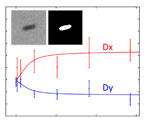
In order to investigate how the external electric field affects the translational diffusion coefficient of the CNTs, in figure 4 we have plotted  $D_x$ and
  $D_y$ as a function of the field strength squared and the alignment energy over
  $k_BT$ similar to figure 3. The predicted theoretical values are also presented here with the fluid viscosity as an adjustable parameter. The experimental results are in good agreement with the model predictions, both of which indicate that the CNTs show anisotropic diffusion behaviour under an aligning electric field. In particular, as we increase the field strength, the
  $x$-direction diffusion coefficient increases while the
  $y$-direction diffusion coefficient decreases. For the specific parameters of this experiment, the diffusion coefficient in the alignment direction increases by approximately 30 % and the diffusion coefficient in the perpendicular directions decreases by 20 %, with both curves saturating for field strengths giving alignment energies exceeding
  $3k_BT$. The error bars indicate the standard deviation of the mean of the measured diffusion coefficients. The experimental variations may be due to uncertainties in CNT dimensions, as well as uncertainties introduced in the image processing and by out-of-plane motion of the CNTs.

Figure 4. Predicted and measured anisotropic diffusion of CNTs in mineral oil under an aligning potential field.
To study the role of CNT dimensions in their observed anisotropic diffusion behaviour, we have also plotted the  $D_x$ and
  $D_y$ as a function of
  $\ln (e)/e$ of the CNT in figure 5 at a given field strength of 33.3
  $\textrm {V}\,\textrm {mm}^{-1}$. The term
  $\ln (e)/e$ is chosen based on (2.35) in the modelling part which reveals the dependence of diffusion on the CNT dimensions. As indicated by the solid lines in figure 5, the model predicts that both
  $D_x$ and
  $D_y$ increase with increasing
  $\ln (e)/e$ (or decreasing particle aspect ratio) in an almost linear manner. The experimental data for the diffusion coefficients show a general trend of increasing with CNT aspect ratio that is consistent with the theory. However, the experimental data is too scattered for quantitative comparison with the model, likely because the CNT length range in our experiments is too small to overcome the measurement uncertainties.

Figure 5. Predicted and measured CNT diffusion in  $x$- and
  $y$-directions plotted against
  $\ln (e)/e$ of CNTs.
5. Conclusions
In this work we have developed a theoretical model to describe the diffusion behaviour of a suspended spheroidal particle in fluid. General analytical solutions were obtained, and then specialized to derive formulae for the effective translational diffusion tensor for prolate spheroidal particles under an aligning potential field. Corresponding experiments were carried out where the translational diffusion coefficients of CNTs are measured in mineral oil under an AC electric field using a single-particle tracking technique. Good agreement was observed between experimental and modelling results, both of which show anisotropic diffusion behaviour in which the diffusion coefficient parallel to the field direction ( $D_x$) increases with the field strength, while that perpendicular to the field direction (
 $D_y$) decreases with the field strength, as expected. The theoretical and experimental curves for
  $D_x$ and
  $D_x$ both began to flatten out as the diffusion coefficients become insensitive to the increasing field strength above a dimensionless alignment energy of 3. It is hoped that this work will provide useful insight into laboratory and industrial systems in which anisotropic particle diffusion can play an important role. The theoretical and experimental approach presented here can also be generalized to anisotropic paramagnetic or ferromagnetic particles under magnetic fields, or any other colloidal system with controlled alignment of anisotropic particles.
Supplementary material
Supplementary material is available at https://doi.org/10.1017/jfm.2021.653.
Funding
This work was supported by the National Science Foundation (L.L., grant numbers CMMI-135156, AFOSR-FA9550-16-1-0181), (J.W.S., grant numbers CBET-1604931, CMMI-1762905).
Declaration of interests
The authors report no conflict of interest.
Appendix A. Derivation for the p.d.f.  $P^{s}(\theta )$ in (2.43)

In general, the p.d.f. is initially defined as  $P^{s}({\boldsymbol {\varTheta }})$ in (2.25), which is determined by a conservative potential
  $V^{rr}({\boldsymbol {\varTheta }})$ where
  ${\boldsymbol {\varTheta }}=(\varphi ,\theta )$ is a parameterization of the orientation of a spheroidal particle. By definition, it is straightforward to see
 \begin{equation} \int_{S^{2}} P^{s}({\boldsymbol{\varTheta}}) \,\textrm{d}{\boldsymbol{\varTheta}} =\int_0^{2{\rm \pi}}\int_0^{\rm \pi} P^{s}(\varphi,\theta)\sin\theta\, \textrm{d}\varphi\,\textrm{d}\theta=\int_0^{\rm \pi} 2{\rm \pi} P^{s}(\varphi,\theta)\sin\theta \,\textrm{d}\theta\equiv 1. \end{equation}
 In our work, the conservative potential (alignment energy)  $V^{rr}({\boldsymbol {\varTheta }})$ is defined in (2.37), which only relies on
  $\theta$. Thus, by substituting (2.37) into (2.25), we directly arrive at
 \begin{equation} P^{s}(\varphi,\theta)\propto\exp\left[-\frac{\epsilon_m a^{3}\zeta |{\boldsymbol E}|^{2}\sin^{2}\theta}{k_BT}\right], \end{equation}
which implies the p.d.f.  $P^{s}({\boldsymbol {\varTheta }}):=P^{s}(\varphi ,\theta )$ of the orientation is only dependent on
  $\theta$.
Based on (A2), to solely consider the p.d.f. in  $\theta$-space, i.e.
  $[0,{\rm \pi} ]$, we have to define
 \begin{equation} P^{s}(\theta):= d \sin\theta \exp\left[-\frac{\epsilon_m a^{3}\zeta |{\boldsymbol E}|^{2}\sin^{2}\theta}{k_BT}\right], \end{equation}
due to (A1). Here  $d$ is a constant that guarantees
 \begin{equation} \int_0^{\rm \pi} P^{s}(\theta)\,\textrm{d}\theta\equiv 1. \end{equation}
Substituting (A3) into (A4) yields
 \begin{equation} d=\dfrac{1}{\int_0^{\rm \pi} \exp\left[-\dfrac{\epsilon_m a^{3}\zeta |{\boldsymbol E}|^{2}\sin^{2}\theta}{k_BT}\right] \sin\theta \,\textrm{d}\theta}, \end{equation}
and thus inserting (A5) back into (A3) generates
 \begin{equation} P^{s}(\theta)=\dfrac{\sin \theta\exp\left[-\dfrac{\epsilon_m a^{3}\zeta |{\boldsymbol E}|^{2}\sin^{2}\theta}{k_BT}\right]}{\int_0^{\rm \pi} \exp\left[-\dfrac{\epsilon_m a^{3}\zeta |{\boldsymbol E}|^{2}\sin^{2}\theta }{k_BT}\right]\sin \theta \,\textrm{d}\theta}, \end{equation}
which is exactly (2.43).


